Heavy quark masses from the $Q\bar{Q}$ threshold and the upsilon expansion

Abstract

Recent results from studies using half the perturbative mass of heavy quark-antiquark $n=1$, ${}^{3}S_{1}$ quarkonium as a new heavy quark mass definition for problems where the characteristic scale is smaller than or of the same order as the heavy quark mass are reviewed. In this new scheme, called the $1S$ mass scheme, the heavy quark mass can be determined very accurately, and many observables like inclusive B decays show nicely converging perturbative expansions. Updates on results using the $1S$ scheme due to new higher order calculations are presented.

1 INTRODUCTION

The top and bottom quark masses are very important phenomenological quantities. Two prominent examples which illustrate that we need to know them to a high degree of precision are virtual top quark effects in electroweak precision observables and B decay phenomenology: the top quark indirectly affects the relation between the $W$, $Z$ masses, and the weak mixing angle $\theta_{W}$ through loop effects which are usually parameterised by the quantity $\Delta\rho\sim m_{t}^{2}G_{F}$. Future improvements in the determination of $M_{W}$ at the Large Hadron Collider (LHC) and Linear Collider (LC) make it desirable to push the error in the top quark mass much below the level of a GeV in order to get stringent bounds on the Higgs boson mass which enters the relation among the electroweak precision observables only logarithmically. Thus the analysis of electroweak precision observables is complementary to direct Higgs searches and provides an important test of electroweak symmetry breaking. The bottom quark mass enters the inclusive B meson decay rates as the fifth power, $\Gamma\sim m_{b}^{5}|V_{CKM}|^{2}$. Thus, the errors in the bottom quark mass should be at the percent level (i.e. not more than 50 MeV), if CKM matrix elements like $V_{cb}$ shall be determined with an error of a few percent from inclusive decays.

Using continuum QCD and perturbative methods the most accurate and precise determinations of the top and bottom quark masses have and will come from observables involving the $t\bar{t}$ and $b\bar{b}$ thresholds. Whereas hadron colliders, which determine the top quark mass from a reconstructed b-W invariant mass distribution, will have a very hard time to reduce the top mass error below 2 GeV due to large systematic uncertainties, a lineshape scan of the total (colour singlet) $t\bar{t}$ cross section close to threshold at the LC will easily determine the top mass with a combined statistical and systematical experimental uncertainty of order 100 MeV [2]. The question is whether one can provide a theoretical description of the threshold lineshape which allows for theoretical uncertainties in the top mass extraction of the same order (or maybe better). For the bottom quark mass, on the other hand, the most precise determinations come from sum rule calculations using the experimental data on the $\Upsilon$ mesons [3]. A quick look at the presently available bottom quark mass determinations [3], however, seems to indicate that a bottom quark mass uncertainty of around 50 MeV is out of question. Observing the spread of numbers given in [3] an uncertainty of 150-200 MeV seems to be more realistic.

On the other hand, when talking about quark masses we have to keep in mind that, due to confinement, they are not observables, but parameters multiplying the bilinear $\bar{\psi}\psi$ operators in the QCD Lagrangian. Thus, they are always determined indirectly, and our ability to determine them with high precision and their usefulness for practical applications can depend on the cleverness of their definition. In this talk I report on recent studies using half the perturbative contributions of a heavy quark-antiquark $n=1$, ${}^{3}S_{1}$ bound state as a new heavy quark mass definition. This new scheme is called the $1S$ scheme [4, 5]. The $1S$ mass is a short-distance mass, i.e. it does not contain an ambiguity of order $\Lambda_{QCD}$ and the problem of large higher order corrections associated with a pole in the Borel transform at $u=1/2$ like the pole mass. But, unlike the well known $\overline{\mbox{MS}}$ mass, which we might consider as the proto-type of a short-distance mass, the $1S$ mass is specialised for problems where the characteristic scale is smaller than the quark mass – a region where the $\overline{\mbox{MS}}$ mass loses its conceptual meaning. By construction, the $1S$ scheme is the optimal choice for problems involving non-relativistic $t\bar{t}$ and $b\bar{b}$ systems, and one can expect that the $1S$ mass can be determined from them with small uncertainties. I will demonstrate the advantages of the $1S$ mass compared to the pole and the $\overline{\mbox{MS}}$ scheme for the NNLO calculations of the total $t\bar{t}$ cross section close to threshold at the LC [4] and a sum rule determination of the bottom quark mass [5]. However, the $1S$ mass scheme also works well for non-$Q\bar{Q}$ problems like inclusive $B$ meson decays. It also allows for a more refined determination of the $\overline{\mbox{MS}}$ mass. If the $1S$ scheme would not be applicable for non-$Q\bar{Q}$ system it would be of little practical value. In order to apply the $1S$ mass scheme to non-$Q\bar{Q}$ systems a modified perturbative expansion, called the upsilon expansion [6], has to be employed. I hope that the $1S$ scheme can contribute to the general acceptance that the desired top and bottom quark mass uncertainties mentioned above are realistic and can indeed be achieved, although the $1S$ scheme is certainly not the only way to achieve this aim. At the end of this talk I will also comment on other low scale short-distance masses that can be found in literature and their relation to the $1S$ mass.

2 THE $1S$ MASS

The $1S$ heavy quark mass is defined as half the perturbative contribution of a $J^{PC}=1^{--}$, ${}^{3}\!S_{1}$ $Q\bar{Q}$ ground state mass. Expressed in terms of the pole mass the $1S$ mass at NNLO in the non-relativistic expansion reads ($a_{s}=\alpha_{s}^{(n_{l})}(\mu)$), [7, 8]

$$M^{1S}=M^{pole}[1-\epsilon\,\Delta^{\mbox{\tiny LO}}-\epsilon^{2}\,\Delta^{\mbox{\tiny LO}}\delta^{1}-\epsilon^{3}\,\Delta^{\mbox{\tiny LO}}\delta^{2}]\,,$$ (1)

where

$$\Delta^{\mbox{\tiny LO}} = \mbox{$\frac{C_{F}^{2}a_{s}^{2}}{8}$}\,,$$ (2)

$$\delta^{1} = \mbox{$(\frac{a_{s}}{\pi})[\beta_{0}(L+1)+\frac{a_{1}}{2}]$}\,,$$ (3)

$$\delta^{2} = (\frac{a_{s}}{\pi})^{2}[\beta_{0}^{2}(\frac{3}{4}L^{2}+L+\frac{\zeta_{3}}{2}+\frac{\pi^{2}}{24}+\frac{1}{4})$$ (4)

$$\quad+\beta_{0}\frac{a_{1}}{2}(\frac{3}{2}L+1)+\frac{\beta_{1}}{4}(L+1)$$

$$\mbox{$\quad+\frac{a_{1}^{2}}{16}+\frac{a_{2}}{8}+(C_{A}-\frac{C_{F}}{48})C_{F}\pi^{2}]$}\,,$$

$$L \equiv \mbox{$\ln(\frac{\mu}{C_{F}a_{s}M^{pole}})$}\,,$$ (5)

and

$$a_{1} = \mbox{$\frac{31}{9}C_{A}-\frac{20}{9}Tn_{l}$}\,,$$

$$a_{2} = (\frac{4343}{162}+4\pi^{2}-\frac{\pi^{4}}{4}+\frac{22}{3}\zeta_{3})C_{A}^{2}$$ (6)

$$\quad-(\frac{1798}{81}+\frac{56}{3}\zeta_{3})C_{A}Tn_{l}$$

$$\mbox{$\quad-(\frac{55}{3}-16\zeta_{3})C_{F}Tn_{l}+(\frac{20}{9}Tn_{l})^{2}$}\,.$$

The constants $\beta_{0}=11-\frac{2}{3}n_{l}$ and $\beta_{1}=102-\frac{38}{3}n_{l}$ are the one- and two-loop coefficients of the QCD beta function and the constants $a_{1}$ [9, 10] and $a_{2}$ [11] the non-logarithmic one- and two-loop corrections to the static colour-singlet heavy quark potential in the pole mass scheme, $V^{Coul}$. All $n_{l}$ light quarks are treated as massless. In Eq. (1) we have labelled the contributions at LO, NLO and NNLO in the non-relativistic expansion by powers $\epsilon$, $\epsilon^{2}$ and $\epsilon^{3}$, respectively, of the auxiliary parameter $\epsilon=1$. The meaning will become clear when we introduce the upsilon expansion later in this talk.

$M^{1S}$ is a short-distance mass because it contains, by construction, half of the total static energy $\langle 2M_{b}^{pole}+V^{Coul}\rangle$ which can be proven to be free of ambiguities of order $\Lambda_{QCD}$ [12, 13] (see also [14]). The fact that the static potential is sensitive to scales below the inverse Bohr radius [15] does not lead to ambiguities because the $1S$ mass also contains the physical perturbative contributions from momenta below the inverse Bohr radius.

3 APPLICATION TO $Q\bar{Q}$ SYSTEMS – $1S$ MASS DETERMINATION

Within the last two years there has been significant progress in our ability to calculate higher order corrections to non-relativistic $Q\bar{Q}$ systems. For the case that the average energy of the quarks is (much) larger than $\Lambda_{QCD}$ NNLO corrections (i.e. corrections of order $\alpha_{s}^{2}$, $\alpha_{s}v$ and $v^{2}$) are now available for the production cross section of $Q\bar{Q}$ pairs in the threshold region. The conceptual framework in which those perturbative calculations can be organised in an economical way is (P)NRQCD, an non-relativistic effective field theory of QCD. Two talks about this subject are given on this conference [16]. The newly available NNLO corrections clearly demonstrate the need for the introduction of a low scale short-distance mass like the $1S$ mass, if the desired quark mass uncertainties mentioned before shall be achieved.

3.1 $t\bar{t}$ production at threshold

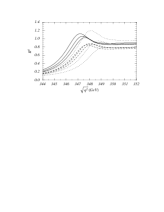
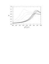
Figure 1: The total normalised vector-current-induced $t\bar{t}$ cross section at the LC versus the c.m. energy in the threshold regime at LO (dotted curves), NLO (dashed) and NNLO (solid) in the pole (upper figure), $\overline{\mbox{MS}}$ (middle) and $1S$ (lower) mass schemes for $\alpha_{s}(M_{Z})=0.118$ and $\mu=15$, $30$, $60$ GeV. The plots have been generated from results obtained in [17, 4]. NNLO calculations for the cross section have also been carried out in [18, 19, 20, 21, 22].

In Figs. 1 the total photon-mediated $t\bar{t}$ cross section in the threshold region at the LC normalised to the muon pair cross section,

$$R^{\gamma}\,\equiv\,\frac{\sigma(e^{+}e^{-}\to\gamma^{*}\to t\bar{t})}{\sigma(e^{+}e^{-}\to\gamma^{*}\to\mu^{+}\mu^{-})}\,,$$ (7)

is displayed at LO, NLO and NNLO for three different renormalisation scales. The three figures show the cross section in the pole (upper figure), the $\overline{\mbox{MS}}$ (middle) and the $1S$ (lower) mass schemes for $(M_{t}^{pole},\overline{m}_{t}(\overline{m}_{t}),M_{t}^{1S})=(175,165,175)$ GeV. To implement the $\overline{\mbox{MS}}$ mass scheme (here and also in the $\Upsilon$ sum rule analysis) the upsilon expansion (Sec. 4.1) has been employed. We see that in the pole mass scheme the location of the peak does not show any sign of convergence. In the $\overline{\mbox{MS}}$ mass scheme the peak location converges, but at the cost of even larger corrections. The figures show that it is very hard to determine the pole or the $\overline{\mbox{MS}}$ mass with theoretical uncertainties below half a GeV. Compared to the best results expected from hadron colliders the situation is not bad, but we can do much better. The situation improves dramatically in the $1S$ scheme, where the peak position is absolutely stable. Realistic simulation studies [2] have shown that the $1S$ mass can be extracted from the threshold scan with theoretical uncertainties of order 100 MeV. Those studies have taken into account beamstrahlung effects that lead to a smearing of the cross section and the fact that the remaining normalisation uncertainties affect the top mass determination.

3.2 $\Upsilon$ mesons

The $\Upsilon$ sum rules relate moments of the the correlator of two electromagnetic bottom quark currents

$$P_{n}^{th}\,=\,\mbox{$\frac{4\,\pi^{2}}{9\,n!\,q^{2}}(\frac{d}{dq^{2}})^{n}\,{\Pi^{b\bar{b}}}_{\mu}^{\,\,\mu}(q)\big{|}_{q^{2}=0}$}$$ (8)

to a dispersion integral over the total $b\bar{b}$ production cross section in $e^{+}e^{-}$ annihilation,

$$P_{n}\,=\,\mbox{$\int^{\infty}_{\sqrt{s}_{min}}\frac{ds}{s^{n+1}}\,R^{b\bar{b}}(s)$}\,.$$ (9)

For values of $n$ between about 4 and 10 the moments are saturated by the non-relativistic $b\bar{b}$ bound states and, at the same time, can be calculated perturbatively at NNLO in the non-relativistic expansion. Choosing $\alpha_{s}$ as an input, and assuming global duality, the $b$ quark mass can be extracted from fits to the experimental data [23, 5].

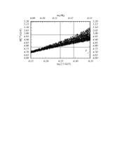
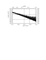
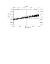
Figure 2: The dark regions show the allowed bottom mass values as a function of $\alpha_{s}$ using NNLO $\Upsilon$ sum rules in the pole (upper figure), $\overline{\mbox{MS}}$ (middle) and $1S$ (lower figure) mass schemes. The diagrams have been generated from results obtained in [23, 5]. Mass extractions for $\alpha_{s}(M_{Z})=0.118\pm 0.004$ are indicated. Sum rule analyses at NNLO have also been carried out in [8, 24, 25].

In Figs. 2 the results for the pole (upper figure), $\overline{\mbox{MS}}$ (middle) and $1S$ (lower) mass at NNLO from a simultaneous fit of four different moments with $4<n<10$ are displayed as a function of the strong coupling. To obtain the error band many individual 95% CL fits have been carried out for random choices of the other theoretical parameters. The width of the error bands is dominated by variations of the renormalisation scale in the QCD potential. The shown spread has been obtained by randomly choosing values above $1.5$ GeV. We see that the pole and the $\overline{\mbox{MS}}$ mass analysis lead to mass extractions which are strongly correlated to the value of $\alpha_{s}$ and which have uncertainties of 100 MeV. In the $1S$ scheme, on the other hand, the correlation to $\alpha_{s}$ and also the uncertainty is much smaller. Using $\alpha_{s}(M_{Z})=0.118\pm 0.004$ as input we obtain $M_{b}^{1S}=4.71\pm 0.03$ GeV for the $1S$ mass, where the error should be considered as $1\sigma$.

This result can be cross-checked by using the fact that twice the $1S$ bottom mass is equal to the mass of the $\Upsilon(1S)$ meson up to non-perturbative corrections:

$$M_{b}^{1S}\,=\,\mbox{$\frac{1}{2}M_{\Upsilon(1S)}-\frac{1}{2}\Delta_{\Upsilon(1S)}^{\rm non-pert}$}\,.$$ (10)

Because quantitative calculations for $\Delta_{\Upsilon(1S)}^{\rm non-pert}$ do not exist yet one can only estimate its size and treat the estimate as an uncertainty. Such estimates, using e.g. the gluon condensate contribution to an ultra-heavy quarkonium, indicate that $\Delta_{\Upsilon(1S)}^{\rm non-pert}$ is not larger than 100 MeV (see e.g. [6]). This estimate leads to

$$M_{b}^{1S}\,=\,\mbox{$4.73\pm 0.05\,\mbox{GeV}$}\,,$$ (11)

which is perfectly consistent with the much more complicated sum rule determination. [(P)NRQCD counting rules indicate that non-perturbative effects associated with retardation effects are of NNLO in the nonrelativistic expansion in the $b\bar{b}$ system [16]; i.e. they should be of the order of the $\epsilon^{3}$ terms shown in Eq. (18) which is consistent with Eq. (11).] The error in Eq. (11) should be considered as $1\sigma$. In fact, we can also consider the sum rule calculation, where non-perturbative effects are much smaller than for the individual $\Upsilon(1S)$ bound state, as a confirmation that the non-perturbative contributions in the $\Upsilon(1S)$ mass are indeed as small as mentioned before. We emphasise, however, that the sum rule determination of $M_{b}^{1S}$ and the result obtained in Eq. (11) are not independent. We use the result in Eq. (11) for the rest of this talk.

4 $1S$ MASS AND NON-$Q\bar{Q}$ SYSTEMS

4.1 The upsilon expansion

The series defining the $1S$ mass, Eq. (1), starts with order $\alpha_{s}^{2}$ because the binding energy of a Coulombic $Q\bar{Q}$ system is of order $M_{Q}v^{2}\sim M_{Q}\alpha_{s}^{2}$. This feature raises the question, how the $1S$ mass has to be implemented into calculations for non-Coulombic quantities. The guiding principle for the implementation of the $1S$ mass into these systems is that the cancellation of the most infrared sensitive contributions contained in Eq. (1) has to be guaranteed after elimination of the pole mass. This is achieved by the upsilon expansion [6]. In the upsilon expansion terms of order $\alpha_{s}^{n}$ in non-Coulombic quantities are of order $\epsilon^{n}$, whereas in Eq. (1) they are of order $\epsilon^{n-1}$. To implement the $1S$ mass one then has to eliminate the pole mass and expand in the parameter $\epsilon$, which is set to one afterwards. In other words, the upsilon expansion combines those orders where the maximal power of $n_{l}$ is the same. Thus the upsilon expansion combines terms of different order in $\alpha_{s}$. This unusual prescription can be understood from the fact that the leading IR-sensitive contributions in Eq. (1) (i.e. those contributions involving the highest power of $\beta_{0}$ in each order) contain powers of the logarithmic term $L=\ln(\mu/C_{F}\,a_{s}\,M_{b}^{pole})$. These logarithmic terms exponentiate at larger orders, $\sum_{i=0}L^{i}/i!\approx\exp(L)=\mu/C_{F}\,a_{s}\,M_{b}^{pole}$, and effectively cancel one power of $\alpha_{s}$ [6]. In the following I will present a number of examples showing that the $1S$ scheme, using the upsilon expansion, leads to nicely converging perturbative series. Keeping in mind that the $1S$ mass can be determined very accurately, this makes the $1S$ mass a very useful scheme for phenomenological applications.

4.2 Inclusive B decays

In Refs. [6] the $1S$ scheme has been applied for all inclusive B decay rates and some exclusive ones. In this talk I only report on the inclusive semileptonic $B\to X_{c}e\bar{\nu}$ and $B\to X_{u}e\bar{\nu}$ decay rates, which are relevant for the determination of the CKM matrix elements $|V_{cb}|$ and $|V_{ub}|$.

At order $\epsilon^{2}$ in the $1S$ scheme the inclusive semileptonic $b\to u$ decay rate reads

$$\Gamma_{B\to X_{u}e\bar{\nu}}\,=\,\mbox{$\frac{G_{F}^{2}|V_{ub}|^{2}}{192\pi^{3}}(M_{b}^{1S})^{5}\times$}$$

$$\mbox{$\times[1-0.115\epsilon-0.031\epsilon^{2}-\frac{9\lambda_{2}-\lambda_{1}}{2(M_{b}^{1S})^{2}}+\ldots]$}\,.$$

The order $\epsilon^{2}$ term is exact [26]. For comparison, the first three terms in the brackets in the pole mass scheme are $[1-0.17\epsilon-0.10\epsilon^{2}]$. Using the $\overline{\mbox{MS}}$ mass they read $[1+0.30\epsilon+0.13\epsilon^{2}]$. Using Eq. (11) for the $1S$ mass and $\lambda_{2}=0.12\,{\rm GeV}^{2}$ and $\lambda_{1}=(-0.25\pm 0.25)\,{\rm GeV}^{2}$ for the chromomagnetic and the kinetic energy matrix elements Eq. (4.2) implies

$$|V_{ub}| = (3.04\pm 0.08\pm 0.08)\times 10^{-3}\times$$ (13)

$$\mbox{$\times\left({{\cal B}(B\to X_{u}e\bar{\nu})\over 0.001}{1.6\,{\rm ps}\over\tau_{B}}\right)^{1/2}$}\,.$$

The first error is obtained by assigning an uncertainty in Eq. (4.2) equal to the value of the $\epsilon^{2}$ term and the second is from assuming the 50 MeV uncertainty in $M_{b}^{1S}$. The scale dependence of $|V_{ub}|$ due to varying $\mu$ in the range $m_{b}/2<\mu<2m_{b}$ is less than 1%. The uncertainty in $\lambda_{1}$ makes a negligible contribution to the total error. It is not easy to measure ${\cal B}(B\to X_{u}e\bar{\nu})$ without significant experimental cuts, for example, on the hadronic invariant mass. Using the $1S$ scheme should reduce the uncertainties in such analyses as well.

At order $\epsilon^{2}$ the inclusive semileptonic $b\to c$ decay rate reads [6]

$$\Gamma(B\to X_{c}e\bar{\nu})=\frac{G_{F}^{2}|V_{cb}|^{2}}{192\pi^{3}}(M_{b}^{1S})^{5}\times 0.533\times$$

$$[1-0.096\epsilon-0.029_{\tiny\rm BLM}\epsilon^{2}-\frac{0.28\lambda_{2}+0.12\lambda_{1}}{\rm GeV^{2}}\ldots].$$

For comparison, the perturbation series in this relation, when written in terms of the pole mass, is $[1-0.12\epsilon-0.07_{\rm BLM}\epsilon^{2}]$. Eq. (4.2) implies

$$|V_{cb}| = (41.6\pm 0.8\pm 0.7\pm 0.5)\times 10^{-3}\times$$ (15)

$$\mbox{$\times\eta_{\rm QED}\left({{\cal B}(B\to X_{c}e\bar{\nu})\over 0.105}\,{1.6\,{\rm ps}\over\tau_{B}}\right)^{1/2}$}\,,$$

where $\eta_{\rm QED}\sim 1.007$ is the electromagnetic radiative correction. The uncertainties come from assuming an error in Eq. (4.2) equal to the $\epsilon^{2}$ term, the $0.25\,{\rm GeV}^{2}$ error in $\lambda_{1}$, and the 50 MeV error in $M_{b}^{1S}$, respectively. The agreement of $|V_{cb}|$ with other determinations (such as exclusive decays) provides an additional check that nonperturbative corrections in $M_{\Upsilon(1S)}$ are indeed small.

4.3 The top width and $\Delta\rho$

It is illustrative to also examine the QCD corrections to the top quark width, $\Gamma_{t}$, and to the top quark corrections to $\Delta\rho$ parameter. One might think that using the $1S$ mass for the top decay width might lead to an improvement similar to the inclusive B decay rates. However, one has to keep in mind that the top decays into a real W boson, which makes the rate only depending on the third power of the top mass, and that the overall renormalisation scale is much higher, which makes the strong coupling quite small. Thus, using the $1S$ scheme, we might expect an improvement in the convergence of the series compared to the pole mass scheme, but it is not clear whether the $1S$ mass beats the $\overline{\mbox{MS}}$ mass. (We also have to keep in mind that for $\Gamma_{t}$ and $\Delta\rho$ even the pole mass leads to an acceptable behaviour of the perturbative series.) For simplicity we only consider the limit $M_{W}=0$. Choosing $\alpha_{s}=0.11$ at the scale of the top mass the top decay width in pole mass scheme reads [27, 28] $\Gamma_{t}(t\to bW)=\Gamma_{0}^{pole}[1-0.10\epsilon-0.02\epsilon^{2}]$, where $\Gamma_{0}\equiv\frac{G_{F}m_{t}|V_{tb}|^{2}}{8\pi\sqrt{2}}$. In the $1S$ mass scheme the series is $\Gamma_{t}=\Gamma_{0}^{1S}[1-0.09\epsilon-0.01\epsilon^{2}]$, and using the $\overline{\mbox{MS}}$ mass (at the $\overline{\mbox{MS}}$ mass) we have $\Gamma(t\to bW)=\bar{\Gamma}_{0}[1-0.04\epsilon-0.003\epsilon^{2}]$. We see that the $1S$ mass leads to a better convergence than the pole scheme, but in the $\overline{\mbox{MS}}$ mass scheme we arrive at the best result. The situation is similar for $\Delta\rho$. In the massless W limit and for $\alpha_{s}=0.11$ at the top mass scale the QCD corrections to the top mass contributions in the $\Delta\rho$ in the pole mass scheme are $\Delta\rho=x_{t}^{pole}[1-0.098\epsilon-0.017\epsilon^{2}]$, where $x_{t}\equiv 3\frac{G_{F}m_{t}^{2}}{8\sqrt{2}\pi^{2}}$. In the $1S$ scheme we have $\Delta\rho=x_{t}^{1S}[1-0.095\epsilon-0.014\epsilon^{2}]$, and using the $\overline{\mbox{MS}}$ mass (at the $\overline{\mbox{MS}}$ mass) the result reads $\Delta\rho=\bar{x}_{t}[1-0.007\epsilon-0.007\epsilon^{2}]$. As for the case of $\Gamma_{t}$ the $\epsilon^{2}$ term is a factor of two larger in the $1S$ scheme than in the $\overline{\mbox{MS}}$ scheme. This observation seems to favour the use of the $\overline{\mbox{MS}}$ mass, but, as we will show just below, it does not necessarily lead to smaller uncertainties because the error in $\overline{\mbox{MS}}$ mass is always larger than the error in the $1S$ mass.

4.4 Determination of $\overline{\mbox{MS}}$ masses

By construction, the $1S$ mass does not know much about large momenta above the inverse Bohr radius $\sim M_{Q}\alpha_{s}$. Thus it cannot be expected to serve as a practical mass prescription for high energy processes where the renormalisation point is well above the heavy quark mass. For those systems the $\overline{\mbox{MS}}$ mass is undeniably one of the best choices. (A well known example is $e^{+}e^{-}$ annihilation into massive quarks at high energies, where the use of the $\overline{\mbox{MS}}$ mass leads to the cancellation of certain large logarithms.) Nevertheless, an accurate determination of the $1S$ mass can also provide a refined determination of the $\overline{\mbox{MS}}$ mass at a low, but still reasonable, scale of order the heavy quark mass. The obtained result for the $\overline{\mbox{MS}}$ mass can then be evolved up to the characteristic scale of the high energy process.

To determine the $\overline{\mbox{MS}}$ mass from $M_{b}^{1S}$ we again have to employ the upsilon expansion. We emphasise that in order to obtain the relation between the $\overline{\mbox{MS}}$ mass and $M_{b}^{1S}$ to order $\epsilon^{3}$ we need the relation between the $\overline{\mbox{MS}}$ and the pole mass to three loops. Whereas the one and two loop corrections are known for quite a while, a numerical calculation of the three loop terms has just been announced on this conference  [29, 30]. The result obtained in Ref. [30] reads ($\overline{m}\equiv\overline{m}^{(n_{l}+1)}$, $a\equiv\alpha_{s}^{n_{l}+1}(\overline{m}(\overline{m}))$)

$$M^{pole}\,=\,\overline{m}(\overline{m})[\,1+0.4243\,a\,\epsilon$$

$$+a^{2}\,(1.362-0.1055n_{l})\,\epsilon^{2}$$

$$\quad+a^{3}\,(6.26(16)-0.871(22)n_{l}+0.02106n_{l}^{2})\,\epsilon^{3}\,]\,.$$

Combining Eqs. (1) and (4.4) we arrive at ($\bar{a}\equiv\alpha_{s}^{(n_{l})}(M^{1S})$, $\ell\equiv\ln\bar{a}$)

$$\overline{m}(\overline{m})\,=\,M^{1S}\{1+[-0.4243\bar{a}+0.2222\bar{a}^{2}]\epsilon$$

$$+[0.0494\bar{a}^{4}+\bar{a}^{2}(-1.18+0.106n_{l})$$

$$\quad+\bar{a}^{3}(0.825-0.778\ell+(-0.0729+0.0472\ell)n_{l})]\epsilon^{2}$$

$$+[\bar{a}^{3}(-5.5(2)+0.80(2)n_{l}-0.021n_{l}^{2})$$

$$\quad+\bar{a}^{4}(5.8-3.7\ell+2.0\ell^{2}$$

$$\qquad+(-0.69+0.56\ell-0.25\ell^{2})n_{l}$$

$$\qquad+(0.020-0.018\ell+0.0075\ell^{2})n_{l}^{2})$$

$$\quad+\bar{a}^{5}(0.21-0.35\ell+(-0.022+0.021\ell)n_{l})$$

$$\quad+0.011\bar{a}^{6}]\epsilon^{3}\}\,.$$ (17)

Using the value for bottom $1S$ mass displayed in Eq. (11) we arrive at

$$\overline{m}_{b}(\overline{m}_{b})=\mbox{$[4.73-0.38\,\epsilon-0.10\,\epsilon^{2}-0.04\,\epsilon^{3}$}$$ (18)

$$\qquad\mbox{$\pm 0.05(\delta M_{b}^{1S})\pm x\,0.01(\delta\alpha_{s})]$~{}GeV}\,.$$

The good convergence of the terms in the upsilon expansion is expected because both the $1S$ and $\overline{\mbox{MS}}$ masses are short-distance masses, i.e. their relation does not have the bad high order behaviour that plagues the pole mass. In Eq. (18) also the error from the uncertainty in the strong coupling is displayed assuming $\alpha_{s}(M_{Z})=0.118\pm x\,0.001$. For $x=4$ this amounts to an error of 40 MeV, which is as large as the $\epsilon^{3}$ term. This uncertainty is nothing else than the strong correlation visible in the lower picture of Fig. 2. It cannot be eliminated, unless the uncertainty in the strong coupling is reduced. What we gain, however, by using the $1S$ mass in the first place, is a reduction of the uncertainties arising from the variations of theoretical parameters like the renormalisation scale. (Those uncertainties are associated with the width of the error band in the lower picture of Figs. 2.) Combining the uncertainties quadratically be arrive at

$$\overline{m}_{b}(\overline{m}_{b}) = 4.21\,\pm\,0.07~{}\mbox{GeV}$$ (19)

for the $\overline{\mbox{MS}}$ bottom quark mass. The uncertainty should be considered as $1\sigma$. For the $1S$ mass value obtained from the sum rule analysis we get $\overline{m}_{b}(\overline{m}_{b})=4.19\pm 0.06~{}\mbox{GeV}$. We note that the central value can vary by up to 30 MeV depending on which method one uses to determine the $\overline{\mbox{MS}}$ mass from Eqs. (1) and (4.4). Thus a conversion error of 30 MeV is included in the error estimates.

The same analysis could also be carried out for the top quark mass. So let us assume that the LC has determined the top $1S$ mass as $M_{t}^{1S}=175\pm 0.2$ GeV from the threshold scan. The expression that corresponds to Eq. (18) then reads $\bar{m}_{t}(\bar{m}_{t})=[175-7.50\,\epsilon-0.94\,\epsilon^{2}-0.19\,\epsilon^{3}\pm 0.2(\delta M_{1S})\pm x\,0.07(\delta\alpha_{s})]$ GeV, which would imply $\bar{m}_{t}(\bar{m}_{t})=166.4\pm 0.4$ GeV for $x=4$. Again, the uncertainty in the $\overline{\mbox{MS}}$ mass is larger unless the uncertainty in the strong coupling is significantly reduced.

5 OTHER MASS DEFINITIONS

The idea of using a short-distance mass especially adapted to problems with a low characteristic scale has not been new. In Ref. [31] the so-called “kinetic mass”, defined by a cutoff-dependent subtraction from the heavy quark self energy, has been proposed and used to parameterise inclusive B decays with results similar to the ones shown in this talk. At present, the kinetic mass is only known to order $\epsilon^{2}$ [32]. An analysis using $\Upsilon$ sum rules determining the kinetic mass can be found in Ref. [8]. In Ref. [13] the so called “potential-subtracted” mass, defined by a cutoff-dependent subtraction from the static QCD potential, has been proposed as a mass definition adequate for threshold problems. In Ref. [20] the potential-subtracted mass has been employed to describe $t\bar{t}$ production close to threshold at the LC and in Ref. [25] it has been determined using $\Upsilon$ sum rules. However, because beyond order $\epsilon^{3}$ (=NNLO in the non-relativistic expansion), the static potential is sensitive to scales below the inverse Bohr radius [15], further considerations are required to fully justify its use as a short-distance mass.

It should be emphasised that there are almost an infinite numbers of ways to define low scale short-distance masses, so even more might be invented in the future. In this respect it is very reasonable to use the $\overline{\mbox{MS}}$ mass as a common reference point which allows to check the consistency of those masses. (In fact, using one of the low scale short-distance masses as a reference point would be a smarter choice owing to the loss of precision in the conversion to the $\overline{\mbox{MS}}$ mass scheme.) In the case of bottom quark mass determinations the obtained results for the $\overline{\mbox{MS}}$ mass from $1S$ ($4.21\pm 0.07$ GeV), kinetic ($4.2\pm 0.1$ GeV [8]) and potential-subtracted mass ($4.25\pm 0.08$ GeV [25]) analyses are perfectly consistent. A critical and comprehensive comparison to (and review of) all $\overline{\mbox{MS}}$ bottom mass determinations prior to the ones just mentioned is certainly useful and shall be carried out elsewhere.

6 ACKNOWLEDGEMENTS

I thank Z. Ligeti, A. V. Manohar and T. Teubner for their collaboration on topics reported in this talk. This work is supported in part by the EU Fourth Framework Program “Training and Mobility of Researchers”, Network “Quantum Chromodynamics and Deep Structure of Elementary Particles”, contract FMRX-CT98-0194 (DG12-MIHT).

References

- [1]
- [2] D. Peralta etal., talk presented a International Workshop on Linear Colliders, April 28 - May 5, 1999 Sitges, Barcelona, Spain.
- [3] Particle Data Group, C. Caso et al, Eur. Phys. J. C 3 (1998) 1.
- [4] A. H. Hoang and T. Teubner, hep-ph/9904468.
- [5] A. H. Hoang, hep-ph/9905550.
- [6] A. H. Hoang, Z. Ligeti and A. V. Manohar, Phys. Rev. Lett. 82 (1999) 277; Phys. Rev. D 59 (1999) 074017 [hep-ph/9811239].
- [7] A. Pineda and F. J. Yndurain, Phys. Rev. D 58 (1998) 094022.
- [8] K. Melnikov and A. Yelkhovky, Phys. Rev. D 59 (1999) 114009
- [9] W. Fischler, Nucl. Phys. B 129 (1977) 157.
- [10] A. Billoire, Phys. Lett. B 92 (1980) 343.
- [11] Y. Schröder, Phys. Lett. B 447 (1999) 321.
- [12] A. H. Hoang, M. C. Smith, T. Stelzer and S. Willenbrock, Phys. Rev. D 59 (1999) 114014 [hep-ph/9804227].
- [13] M. Beneke, Phys. Lett. B 434 (1998) 115.
- [14] N. Uraltsev, hep-ph/9804275.
- [15] T. Appelquist, M. Dine and I. J. Muzinich, Phys. Rev. D 17 (1978) 2074.
- [16] A. Pineda; M. Beneke, these proceedings.
- [17] A. H. Hoang and T. Teubner, Phys. Rev. D 58 (1998) 114023 [hep-ph/9801397].
- [18] K. Melnikov and A. Yelkhovsky, Nucl. Phys. B 528 (1998) 59.
- [19] O. Yakovlev, Phys. Lett. B 457 (1999) 170.
- [20] M. Beneke et al, Phys. Lett. B 454 (1999) 137.
- [21] T. Nagano et al, hep-ph/9903498.
- [22] A. A. Penin, and A. A. Pivovarov, hep-ph/9904278.
- [23] A. H. Hoang, Phys. Rev. D 59 (1999) 014039 [hep-ph/9803454].
- [24] A. A. Penin, and A. A. Pivovarov, Phys. Lett. B 435 (1998) 413; Nucl. Phys. B 549 (1999) 217;
- [25] M. Beneke and A. Signer, hep-ph/9906475.
- [26] T. v. Ritbergen, Phys. Lett. B 454 (1999) 353.
- [27] A. Czarnecki and K. Melnikov, Nucl. Phys. B 544 (1999) 520.
- [28] K. G. Chetyrkin et al., hep-ph/9906273.
- [29] K. G. Chetyrkin, these proceedings.
- [30] K. G. Chetyrkin and M. Steinhauser, hep-ph/9907509.
- [31] I. Bigi et al, Phys. Rev. D 56 (1997) 4017.
- [32] A. Czarnecki et al, Phys. Rev. Lett. 80 (1998) 3189.