CP Violating Phases, Nonuniversal Soft Breaking And D-brane Models

Abstract

The question of CP violating phases and electric dipole moments (EDMs)for the electron ($d_{e}$) and the neutron ($d_{n}$) for supergravity models with nonuniversal soft breaking is considered for models with a light ($\stackrel{{\scriptstyle<}}{{\sim}}$1 TeV) mass spectrum and R-parity invariance. As with models with universal soft breaking (mSUGRA) one finds a serious fine tuning problem generally arises for $\theta_{0B}$ (the phase of the B soft breaking parameter at the GUT scale), if the experimental EDM constraints are obeyed and radiative breaking of $SU(2)_{L}\times U(1)_{Y}$ occurs. A D-brane model where $SU(3)_{C}\times U(1)_{Y}$ is associated with one set of 5-branes and $SU(2)_{L}$ with another intersecting set of 5-branes is examined, and the cancellation phenomena is studied over the parameter space of the model. Large values of $\theta_{B}$ (the phase of B at the electroweak scale) can be accommodated, though again $\theta_{0B}$ must be fine tuned. Using the conventional prescription for calculating $d_{n}$, one finds the region in parameter space where the experimental EDM constraints on both $d_{e}$ and $d_{n}$ hold is significantly reduced, and generally requires tan$\beta\stackrel{{\scriptstyle<}}{{\sim}}$5 for most of the parameter space, though there are small allowed regions even for tan$\beta\stackrel{{\scriptstyle>}}{{\sim}}$10. We find the Weinberg three gluon term generally makes significant contributions, and results are sensitive to the values of quark masses.

I Introduction

It has been realized for sometime that supersymmetric (SUSY) models allow for an array of CP violating phases not found in the Standard Model(SM), and that these phases will in general give rise to electric dipole moments (EDMs) of the electron and the neutron which might violate the experimental bounds [1]. The current 90 $\%$ C.L. bounds for $d_{n}$ and 95 $\%$ C.L. bounds for $d_{e}$ are quite stringent [2] :

$$(d_{n})_{exp} < 6.3\times 10^{-26}ecm;\,\,\,\,(d_{e})_{exp}<4.3\times 10^{-27}ecm$$ (1)

While these bounds can always be satisfied by assuming sufficiently small phases (i.e O(10^-2)) and/or a heavy SUSY mass spectrum (i.e.$\stackrel{{\scriptstyle>}}{{\sim}}$1 TeV) , recently it has been pointed out that cancellations may occur allowing for “naturally” large phases (i.e. O(10^-1)) and a light mass spectrum [3] and this has led to considerable analysis both within the MSSM framework [3, 4, 5] and the gravity mediated supergravity (SUGRA) GUT framework [6, 7, 8, 9, 10, 11, 12]. In the latter type models the theory is specified by assigning the SUSY parameters at the GUT scale, and using the renormalization group equations (RGEs), one determines the physical predictions at the electroweak scale ($M_{\rm EW}$) (which we take here to be the t-quark mass, $m_{t}$). Thus in SUGRA models, “naturalness” is to be determined in terms of the GUT parameters.

In a previous paper [12], we examined the minimal model, mSUGRA, which depends on the four universal soft breaking parameters at $M_{G}$ [$m_{0}$(scalar mass), $m_{1/2}$ (gaugino mass), $A_{0}$ (cubic term mass) and $B_{0}$ (quadratic term mass)] and the Higgs mixing parameter $\mu_{0}$. Since $m_{0}$ is real and we can choose phases such that $m_{1/2}$ is real, one has only three phases at the GUT scale in mSUGRA:

$$A_{0} = |A_{0}|e^{i\alpha_{0A}};\,B_{0}=|B_{0}|e^{i\theta_{0B}};\,\mu_{0}=|\mu_{0}|e^{i\theta_{0\mu}}.$$ (2)

In Ref.[12], it was shown that for the t-quark cubic soft breaking parameter at $M_{\rm EW}$, $A_{t}=|A_{t}|e^{i\alpha_{t}}$, the nearness of the t-quark Landau pole automatically suppresses $\alpha_{t}$ (the phase of $A_{t}$ at $M_{\rm EW}$), and one can satisfy the EDM bounds with a light SUSY spectrum for large $\alpha_{0A}$, even $\alpha_{0A}=\pi/2$. However, the situation is more difficult for $\theta_{0B}$. The experimental requirements of Eq.(1) combined with radiative breaking of $SU(2)\times U(1)$ at $M_{\rm EW}$ imply that $\theta_{0B}$ is large i.e. O(1) (unless $\alpha_{0A}$ is small and then all phases are small) and more serious, must be tightly fine tuned unless tan$\beta$ is small (tan$\beta\stackrel{{\scriptstyle<}}{{\sim}}$3). For example, fixing $|A_{0}|$, $m_{0}$ and $m_{1/2}$ to be light and $\alpha_{0A}$ large, one characteristically would find that $\theta_{0B}$ needs to be specified to 1 part in 10⁴ for tan$\beta$=10. Without this fine tuning, the GUT theory would not achieve electroweak symmetry breaking at $M_{\rm EW}$ and/or satisfaction of Eq.(1).

Nonminimal models were also examined in [12] with results similar to the above holding. In this paper we examine the nonminimal models in more detail. We then discuss an interesting D-brane model [13], where the Standard Model gauge group is associated with two 5-branes. This model results in nonuniversal gaugino and scalar masses and is able to allow larger values of $\theta_{B}$ at $M_{\rm EW}$. However, the same fine tuning problem at $M_{G}$ for $\theta_{0B}$ results in this model as well.

Our paper is organized as follows: Sec.2 reviews the basic formulae and notation of the SUGRA GUT models for calculating the EDMs. Sec.3 examines a general class of non universalities. Sec.4. considers the model of [13] and conclusions are given in Sec 5.

II EDMs in SUGRA Models

We consider here supersymmetry GUT models possessing R-parity invariance where SUSY is broken in a hidden sector at a scale above $M_{G}\cong 2\times 10^{16}$ GeV. This breaking is then transmitted by gravity to the physical sector. The GUT group is assumed to be broken to the Standard Model (SM) $SU(3)_{C}\times SU(2)_{L}\times U(1)_{Y}$ at $M_{G}$, but is otherwise unspecified. The gauge kinetic function, $f_{\alpha\beta}$, and Kahler potential, K, can then give rise to nonuniversal gaugino masses at $M_{G}$ which we parametrize by

$$m_{1/2i} = |m_{1/2i}|e^{i\phi_{0i}};\,i=1,2,3.$$ (3)

and we chose the phase convention where $\phi_{02}=0$. We also allow nonuniversal Higgs and third generation masses at $M_{G}$ which can arise from the Kahler potential:

$$m_{H_{1}}^{2} = m_{0}^{2}(1+\delta_{1});\,\,\,\,m_{H_{2}}^{2}=m_{0}^{2}(1+\delta_{2})$$ (4)

$$m_{q_{L}}^{2} = m_{0}^{2}(1+\delta_{3});\,m_{u_{R}}^{2}=m_{0}^{2}(1+\delta_{4});\,m_{e_{R}}^{2}=m_{0}^{2}(1+\delta_{5});$$ (5)

$$m_{d_{R}}^{2} = m_{0}^{2}(1+\delta_{6});\,m_{l_{L}}^{2}=m_{0}^{2}(1+\delta_{7});$$ (6)

where $q_{L}\equiv(\tilde{t}_{L},\,\tilde{b}_{L})$, $u_{R}\equiv\tilde{t}_{R}$, $e_{R}\equiv\tilde{\tau}_{R}$, etc., $m_{0}$ is the universal mass of the first two generations and $\delta_{i}$ are the deviations from this for the Higgs bosons and the third generation. In addition, there may be nonuniversal cubic soft breaking parameters at $M_{G}$:

$$A_{0t} = |A_{0t}|e^{i\alpha_{0t}};\,A_{0b}=|A_{0b}|e^{i\alpha_{0b}};\,A_{0\tau}=|A_{0\tau}|e^{i\alpha_{0\tau}}.$$ (7)

The electric dipole moment $d_{f}$ for fermion f is defined by the effective Lagrangian:

$$L_{f} = -{i\over 2}d_{f}\bar{f}\sigma_{\mu\nu}\gamma^{5}fF^{\mu\nu}$$ (8)

Our analysis follows that of [3]. Thus the basic diagrams leading to the EDMs are given in Fig.1. In addition there are gluonic operators

$$L^{G} = -{1\over 3}d^{G}f_{abc}G_{a\mu\alpha}G_{b\nu}^{\alpha}\tilde{G}_{c}^{\mu\nu}$$ (9)

and

$$L^{C} = -{i\over 2}d^{C}\bar{q}\sigma_{\mu\nu}\gamma^{5}T^{a}qG_{a}^{\mu\nu}$$ (10)

contributing to $d_{n}$ arising from the one loop diagram of Fig.1 (when the outgoing vector boson is a gluon), the two loop Weinberg type diagram[14] and two loop Barr-Zee type diagram[15]. (In Eq.(9), $\tilde{G}^{\mu\nu}_{c}={1\over 2}\epsilon^{\mu\nu\alpha\beta}G_{c\alpha\beta}$, $\epsilon^{0123}=+1$, $T^{a}={1\over 2}\lambda_{a}$, where $\lambda_{a}$ are the SU(3) Gellman matrices and $f_{abc}$ are the SU(3) structure constants). We use naive dimensional analysis[16] to relate these to the electric dipole moments and the QCD factors $\eta^{\rm ED}$, $\eta^{G}$, $\eta^{C}$ to evolve these results to 1 GeV[17]. The quark dipole moments are related to $d_{n}$ using the nonrelativistic quark model to relate the u and d quark moments to $d_{n}$ i.e.

$$d_{n} = {1\over 3}(4d_{d}-d_{u})$$ (11)

and we assume the s-quark mass is 150 MeV. Thus QCD effects produce considerable uncertainty in $d_{n}$ (perhaps a factor of 2-3).

Our matter phase conventions are chosen so that the chargino($\chi^{\pm}$), neutralino($\chi^{0}$) and squark and slepton mass matrices take the following form:

$$M_{\chi^{\pm}} = \left(\matrix{\tilde{m}_{2}&\sqrt{2}M_{W}sin\beta\cr\sqrt{2}M_{W}cos\beta&-|\mu|e^{i\theta}}\right)$$ (12)

$$M_{\chi^{0}} = \left(\matrix{|\tilde{m}_{1}|e^{i\phi_{1}}&0&a&b\cr 0&\tilde{m}_{2}&c&d\cr a&c&0&|\mu|e^{i\theta}\cr b&d&|\mu|e^{i\theta}&0\cr}\right)$$ (13)

and

$$M_{\tilde{q}}^{2} = \left(\matrix{m^{2}_{q_{L}}&e^{-i\alpha_{q}}m_{q}(|A_{q}|+|\mu|R_{q}e^{i(\theta+\alpha_{q})})\cr e^{i\alpha_{q}}m_{q}(|A_{q}|+|\mu|R_{q}e^{-i(\theta+\alpha_{q})})&m^{2}_{q_{R}}}\right).$$ (14)

In the above $a=-M_{Z}sin\theta_{W}cos\beta$, $b=M_{Z}sin\theta_{W}sin\beta$, $c=-cot\theta_{W}a$, $d=-cot\theta_{W}b$, $tan\beta=v_{2}/v_{1}$ ($v_{1,2}=\mid<H_{1,2}>\mid$), $R_{q}=cot\beta(tan\beta)$ for u(d) quarks. All parameters are evaluated at the electroweak scale using the RGEs, e.g. for quark q one has $A_{q}=|A_{q}|e^{i\alpha_{q}}$. (Similar formulae hold for the slepton mass matrices.)

Electroweak symmetry breaking gives rise to Higgs VEVs which we parametrize by

$$<H_{1,2}> = v_{1,2}e^{i\epsilon_{1,2}}.$$ (15)

These enter in the phase $\theta$ appearing in Eqs.(12,13,14)

$$\theta \equiv \epsilon_{1}+\epsilon_{2}+\theta_{\mu}$$ (16)

The Higgs VEVs are calculated by minimizing the Higgs effective potential[18]:

$$V_{eff} = m_{1}^{2}v_{1}^{2}+m_{2}^{2}v_{2}^{2}+2|B\mu|cos(\theta+\theta_{B})v_{1}v_{2}+{g^{2}_{2}\over 8}(v_{1}^{2}+v_{2}^{2})^{2}+{{g^{\prime}}^{2}\over 8}(v_{2}^{2}-v_{1}^{2})^{2}+V_{1}$$ (17)

where $m^{2}_{i}=|\mu|^{2}+m^{2}_{H_{i}}$ and $m_{H_{1,2}}^{2}$ are the Higgs running masses at $M_{\rm EW}$. $V_{1}$ is the one loop contribution.

$$V_{1}={1\over{64\pi^{2}}}\sum_{a}C_{a}(-1)^{2j_{a}}(2j_{a}+1)m_{a}^{4}(ln{m_{a}^{2}\over Q^{2}}-{3\over 2})$$ (18)

where $m_{a}$ is the mass of the a particle of spin $j_{a}$, $Q$ is the electroweak scale (which we take to be $m_{t}$) and $C_{a}$ is the number of color degrees of freedom. In the following we include the full third generation states, $t$, $b$ and $\tau$ in $V_{1}$ which allows us to treat the large tan$\beta$ regime. From Eq.(14) this implies that $V_{1}$ depends only on $\theta+\alpha_{q}$, $\theta+\alpha_{l}$ (though the rotation matrices which diagonalize $M_{\tilde{q}}^{2}$, $M_{\tilde{l}}^{2}$ will depend on $\theta$, $\alpha_{q}$ and $\alpha_{l}$ separately). Minimizing $V_{eff}$ with respect to $\epsilon_{1},\,\epsilon_{2}$. then determines $\theta$:

$$\theta=\pi-\theta_{B}+f_{1}(\pi-\theta_{B}+\alpha_{q},\pi-\theta_{B}+\alpha_{l})$$ (19)

where $f_{1}$ is the one loop correction. In general, $f_{1}$ is small, but can become significant for large tan$\beta$, as discussed in [12].

Minimizing $V_{eff}$ with respect to $v_{1}$ and $v_{2}$ yields two equations which can be arranged in the usual fashion to determine $|\mu|^{2}$ and $|B|$ at $M_{\rm EW}$:

$$|\mu|^{2} = {{\mu^{2}_{1}-tan^{2}\beta\mu^{2}_{2}}\over{tan^{2}\beta-1}}-{1\over 2}M_{Z}^{2}$$ (20)

$$|B| = {1\over 2}sin{2\beta}{m_{3}^{2}\over|\mu|}$$ (21)

where $\mu_{i}^{2}=m_{H_{i}}^{2}+\Sigma_{i}$, $m_{3}^{2}=2|\mu|^{2}+\mu^{2}_{1}+\mu^{2}_{2}$ and $\Sigma_{i}=\partial V_{1}/{\partial v_{i}^{2}}$. Note that $|\mu|$ and $|B|$ depend implicitly on the CP violating phases since the RGE that determines $m_{H_{i}}^{2}$ couple to the $A$ and $\tilde{m}_{i}$ equations, and $\Sigma_{i}$ depend on the phases.

III NonMinimal Models

The renormalization group equations that relate $M_{EW}$ to $M_{G}$ are in general complicated differential equations requiring numerical solution, and all results given here are consequences of accurate numerical integration. Approximate analytic solutions can however be found for low and intermediate tan$\beta$ (neglecting b and $\tau$ Yukawa couplings) and in the SO(10) limit of very large tan$\beta$ (neglecting the $\tau$ Yukawa coupling). These analytic solutions give some insight into the nature of the more general numerical solutions.

For low and intermediate tan$\beta$, the $A_{t}$ and Yukawa RGEs read

$$-{{dA_{t}}\over{dt}} = 6Y_{t}A_{t}+{1\over{4\pi}}(\sum^{3}_{i=1}a_{i}\alpha_{i}\tilde{m}_{i})$$ (22)

$$-{{dY_{t}}\over{dt}} = 6Y_{t}-{1\over{4\pi}}(\sum^{3}_{i=1}a_{i}\alpha_{i})Y_{t}$$ (23)

where $Y_{t}=h_{t}^{2}/{16\pi^{2}}$, $h_{t}$ is the t-quark Yukawa coupling constant and $a_{i}$=(13/15,3,16/3). We follow the sign conventions of Ref.[20], and $t=2ln(M_{G}/Q)$. The solutions of Eqs.(20) can be written as

$$A_{t}(t) = D_{0}A_{0t}-\tilde{H_{2}}+{{1-D_{0}}\over F}\tilde{H}_{3}$$ (24)

where

$$\tilde{H_{2}} = {\alpha_{G}\over{4\pi}}t\sum{{a_{i}|m_{1/2i}|e^{i\phi_{i}}}\over{1+\beta_{i}t}}\equiv\sum_{i}H_{2i}|m_{1/2i}|e^{i\phi_{i}}$$ (25)

and

$$\tilde{H_{3}} = \int^{t}_{0}{dt}^{\prime}E(t^{\prime})\tilde{H_{2}}\equiv\sum H_{3i}|m_{1/2i}|e^{i\phi_{i}}.$$ (26)

Here $D_{0}=1-6(F(t)/E(t))Y(t)$ vanishes at the t-quark Landau pole and hence is generally small i.e. ($D_{0}\stackrel{{\scriptstyle<}}{{\sim}}0.2$ for $m_{t}=175$ GeV). The functions F and E depend on the SM gauge beta functions and are given in [19]. (E=12.3, F=254 for $t=2ln(M_{G}/m_{t})$.) We note the identity[19]

$${1\over F}\sum H_{3i} = t{E\over F}-1\cong 2.1.$$ (27)

and so if we write Eq.(24) as

$$A_{t}(t) = D_{0}A_{0t}+\sum\Phi_{i}|m_{1/2i}|e^{i\phi_{i}}.$$ (28)

the $\Phi_{i}$ are real and $O(1)$. (In the SO(10) large tan$\beta$ limit, one obtains an identical result with the factor 6 replaced 7 in $D_{0}$. Thus Eq.(28) gives a valid qualitative picture over a wide range in tan$\beta$.)

Nonuniversal gaugino masses affect the EDMs in two ways. First, taking the imaginary part of Eq.(28) one has ($\phi_{2}$=0 in our phase convention):

$$|A_{t}(t)|sin{\alpha_{t}} = |A_{0t}|D_{0}{\rm sin}\alpha_{0t}+\sum_{i=1,3}\Phi_{i}|m_{1/2i}|{\rm sin}{\phi_{i}}.$$ (29)

As in the universal case, the smallness of $D_{0}$ suppresses the effects of any large $\alpha_{0t}$ on the electroweak scale phase $\alpha_{t}$. However large gaugino phases $\phi_{i}$ will generally make $\alpha_{t}$ large. Second, Eqs.(13) and (12) show that the phase $\phi_{1}$ enters into the neutralino mass matrix though the chargino mass matrix remains unchanged ($\phi_{2}=0$). Thus the $\phi_{1}$ phase will affect any cancellation occurring between the neutralino and chargino contributions to the EDMs.

Some of the above efffects are illustrated in Figs. 2 and 3, where we plot K vs. the phase $\theta_{B}$ at the electroweak scale for $d_{e}$. Here K is defined by

$$K=log_{10}\mid{d_{f}\over{(d_{f})_{exp}}}\mid$$ (30)

Thus K=0 corresponds to the case where the theory saturates the current experimental EDM bound, while K=-1, would be the situation if the experimental bounds were reduced by a factor of 10. Fig.2 considers universal scalar masses and universal $A_{0}$ with $\alpha_{0A}=\pi/2$ at the GUT scale, and $\phi_{1}=\phi_{3}=-1.1\pi$, -1.3$\pi$, -1.5$\pi$ for tan$\beta$=3. We see that as $|\phi_{1}|$ is increased from $|\phi_{1}|$=1.1$\pi$ to 1.3 $\pi$, the allowed values of $\theta_{B}$ increases significantly since the $\phi_{1}$ phase in Eq. (11) aids the cancellation between the neutralino and the chargino contributions. However, increasing $|\phi_{1}|$ further to $|\phi_{1}|$=1.5$\pi$ over compensates causing the allowed values of $\theta_{B}$ to decrease. Fig. 3 for tan$\beta$=10 shows a similar effect. The experimentally allowed parameters require $K\leq 0$. The allowed range $\Delta\theta_{B}$ of $\theta_{B}$ decreases with tan$\beta$. It is very small for tan$\beta$=10 and is quite small even for tan$\beta$=3.

IV D-Brane Models

Recent advances in string theory leading to possible D=4, N=1 supersymmetric vacua after compactification has restimulated interest in phenomenological string motivated model building. A number of approaches exists including models based on Type IIB orientifolds, Horava-Witten M theory compactification on $CY\times S^{1}/Z_{2}$ and perturbative heterotic string vacua. The existence of open string sectors in Type IIB strings implies the presence of $Dp$-branes, manifolds of p+1 dimensions in the full D=10 space of which 6 dimensions are compactified e.g. on a six torus $T^{6}$. (For a survey of properties of Type IIB orientifold models see [21]). One can build models containing 9 branes (the full 10 dimensional space) plus $5_{i}$-branes, i=1, 2, 3 (each containg two of the compact dimensions) or 3 branes plus 7_i branes, i=1, 2, 3 (each having two compactified dimensions orthogonal to the brane). Associated with a set of n coincident branes is a gauge group U(n). Thus there are large number of ways one might embed the Standard Model gauge group in Type IIB models.

We consider here an interesting model recently proposed [13] based on 9-branes and 5-branes. In this model, $SU(3)_{C}\times U(1)_{Y}$ is associated with one set of 5-branes, i.e. $5_{1}$, and SU(2)_L is associated with a second intersecting set 5₂. Strings starting on 5₂ and ending on 5₁ have massless modes carrying the joint quantum numbers of the two branes (we assume these are the SM quark and lepton doublets, Higgs doublets) while strings beginning and ending on 5₁ have massless modes carrying $SU(3)_{C}\times U(1)_{Y}$ quantum numbers (right quark and right lepton states). A number of general properties of such models have been worked out [21]. Thus to accommodate the phenomenological requirement of gauge coupling constant unification at $M_{G}\cong 2\times 10^{16}$ GeV, one may assume, that $M_{c}$, the compactification scale of the Kaluza-Klein modes obeys $M_{c}=M_{G}$. Above $M_{c}$, the gauge interactions on the 5-branes see a D=6 dimensional space (with Kaluza Klein modes) while above $M_{c}$ gravity sees the full D=10 space. Gravity and gauge unification then is to take place at the string scale $M_{\rm str}=1/{\sqrt{\alpha^{\prime}}}$ given by $M_{\rm str}=(\alpha_{G}M_{c}M_{Planck}/\sqrt{2})^{1/2}\cong 8\times 10^{16}$ GeV (for $\alpha_{G}\cong 1/24$).

The gauge kinetic functions for 9 branes and 5_i-branes are given by [21, 22] $f_{9}=S$ and $f_{5_{i}}=T_{i}$ where S is the dilaton and $T_{i}$ are moduli. The origin of the spontaneous breaking of N=1 supersymmetry and of compactification is not yet understood within this framework. Further, CP violation must also occur as a spontaneous breaking. One assumes these effects can be phenomenologically accounted for by F-components growing VEVs parametrized as [21, 23, 24]

$$F^{S} = {2\sqrt{3}}<{\rm Re}S>{\rm sin}\theta_{b}e^{i\alpha_{s}}m_{3/2}$$ (31)

$$F^{T_{i}} = {2\sqrt{3}}<{\rm Re}T_{i}>{\rm cos}\theta_{b}\Theta_{i}e^{i\alpha_{i}}m_{3/2}$$ (32)

where $\theta_{b}$, $\Theta_{i}$ are Goldstino angles ($\Theta_{1}^{2}+\Theta_{2}^{2}+\Theta_{3}^{2}=1$). CP violation is thus incorporated in the phases $\alpha_{s}$, $\alpha_{i}$. In the following we will assume, for simplicity, that $\Theta_{3}=0$ (i.e. that the 5₃-brane does not affect the physical sector). We also assume isotropic compactification ($<ReT_{i}>$) are equal) to guarantee grand unification at $M_{G}$, and $<ImT_{i}>$=0 so that the spontaneous breaking does not grow a $\theta$-QCD type term.

For models of this type, T-duality determines the Kahler potential [21, 23, 24] and, combined with Eq.(28), generates the soft breaking terms. One finds at $M_{G}$[21, 23, 24]:

$$\tilde{m_{1}} = \sqrt{3}{\rm cos}\theta_{b}\Theta_{1}e^{-i\alpha_{1}}m_{3/2}=\tilde{m_{3}}=-A_{0}$$ (33)

$$\tilde{m_{2}} = \sqrt{3}{\rm cos}\theta_{b}\Theta_{2}e^{-i\alpha_{2}}m_{3/2}$$ (34)

and

$$m_{5_{1}5_{2}}^{2} = (1-{3\over 2}{\rm sin}^{2}\theta_{b})m^{2}_{3/2}$$ (35)

$$m_{5_{1}}^{2} = (1-{3}{\rm sin}^{2}\theta_{b})m^{2}_{3/2}$$ (36)

Here $A_{0}$ is a universal cubic soft breaking mass, $m_{5_{1}5_{2}}^{2}$ are the soft breaking masses for $q_{L}$, $l_{L}$, $H_{1,2}$ and $m_{5_{1}}^{2}$ are for $u_{R}$, $d_{R}$ and $e_{R}$.

We see that the brane models give rise to nonuniversalities that are strikingly different from what one might expect in SUGRA GUT models. Thus it would be difficult to construct a GUT group, which upon spontaneous breaking at $M_{G}$ yields gaugino masses $\tilde{m}_{1}$=$\tilde{m}_{3}\neq\tilde{m}_{2}$, and similarly the above pattern of sfermion and Higgs soft masses. Brane models can achieve the above pattern since they have the freedom of associating different parts of the SM gauge group with different branes.

The above model does not determine the $B$ and $\mu$ parameters. We therefore will phenomenologically parametrize these at $M_{G}$ by

$$B_{0}=|B_{0}|e^{i\theta_{0B}};\,\mu_{0}=|\mu_{0}|e^{i\theta_{0\mu}}.$$ (37)

with two additional CP violating phases $\theta_{0B}$ and $\theta_{0\mu}$. We also set $\alpha_{2}=0$ in the following.

We consider first the electron EDM. (We use the interactions of Ref.[25] including the Erratum on the sign of Eq.(5.5) of Ref.[25]). Fig.4 plots K as a function of $\theta_{B}$ for tan$\beta$=2 (solid), 5 (dashed), 10 (dotted) with phases $\phi_{1}=\phi_{3}=\pi+\alpha_{0A}=-1.25\pi$ and $m_{3/2}=150$ GeV, $\theta_{b}=0.2$, $\Theta_{1}$=0.85. We see that the EDM bounds allow remarkably large values of $\theta_{B}$ in this model even for large tan$\beta$, e.g. $\theta_{B}\cong 0.4$ for tan$\beta$=2 and $\theta_{B}\cong 0.25$ for tan$\beta$=10. (A second allowed region occurring approximately for $\theta_{B}\rightarrow\pi+\theta_{B}$ also exists. However this corresponds to the sign of $\mu$ that is mostly excluded by the $b\rightarrow s\gamma$ data.) Fig.5 shows a similar plot for somewhat smaller phases $\phi_{1}=\phi_{3}=\pi+\alpha_{0A}=-1.1\pi$. Again relatively large phases can exist at the electroweak scale.

As discussed in Ref.[13], the largeness of $\theta_{B}$ is due to an enhanced cancellation between the neutralino and chargino contributions as a consequence of the additional $\phi_{1}$ dependence in Eq.(11), allowing $\theta_{B}$ to be O(1). However, in spite of this, the range in $\theta_{B}$ at the electroweak scale, where the experimental bound $K\leq 0$ is satisfied, is quite small, e.g. from Fig.4, $\Delta\theta_{B}\simeq$0.015 even for tan$\beta$=2. As discussed in Ref[12], this implies that the radiative breaking condition makes the allowed range $\Delta\theta_{0B}$ at the GUT scale very small, particularly for large tan$\beta$. This is illustrated in Figs. 6 and 7. In Fig.6, we have plotted the central value of $\theta_{0B}$ which satisfies $K\leq 0$ as a function of tan$\beta$. Thus $\theta_{0B}$ is generally quite large. In Fig.7 we have plotted the allowed range of $\Delta\theta_{0B}$ satisfying the EDM constraints. One sees that even for small tan$\beta$ the allowed range $\Delta\theta_{0B}$ is very small. Thus as in the mSUGRA model of Ref.[12], one has a serious fine tuning problem at the GUT scale due to the combined conditions of radiative breaking and the EDM bound: $\theta_{0B}$ must be large but very accurately determined by the string model if it is to agree with low energy phenomenology.

The neutron dipole moment is more complicated due to the additional contributions arising from $L^{C}$ and $L^{G}$ of Eqs.(8) and (7). While there are significant uncertainties in the calculation of $d_{n}$ it is of interest to see if the experimental bounds on $d_{n}$ can be achieved in the same region of parameter space as occur in $d_{e}$ above. The fact that the brane model requires $\phi_{3}=\phi_{1}$ allows for the $L^{C}$ gluino contribution to aid in canceling the chargino contribution. This generally aids in broadening the overlap region of joint satisfaction of the $d_{n}$ and $d_{e}$ bounds of Eq.(1). However, in addition to this, there is a contribution from $L^{G}$ from the Weinberg type diagram. While this term is enhanced due to the factor of $m_{t}$, it is a two loop diagram and is suppressed by a factor of $\alpha_{3}^{2}$($g_{3}/{4\pi}$) and in most models is usually a small contribution. However, for the D-brane model where $\phi_{3}=\phi_{1}$, the presence of a large $\phi_{3}$ phase increases the significance of this diagram, reducing the $d_{n}-d_{e}$ overlap region. This is illustrated in Figs.8 where $\Theta_{1}$ is plotted as a function of $\theta_{B}$ for parameters tan$\beta$=2, $m_{3/2}=150$ GeV, $\theta_{b}$=0.2. (LEP189 bounds of $m_{1/2}\stackrel{{\scriptstyle>}}{{\sim}}150$ GeV imply here that $\Theta_{1}\stackrel{{\scriptstyle<}}{{\sim}}0.94$.) As one proceeds from $\phi_{1}=\phi_{3}=-1.25\pi$ of Fig.8a to $\phi_{1}=\phi_{3}=-1.95\pi$ of Fig.8d, one goes from no overlap of the allowed $d_{e}$ and $d_{n}$ regions to a significant overlap. However, the large $\theta_{B}$ phase allowed separately by $d_{e}$ and $d_{n}$ (e.g. $\theta_{B}\sim 0.6$) in Fig.8a is sharply reduced in Fig.8d in the overlap region by a factor of 10. Further, the region of parameter space where the experimental constraints for $d_{e}$ and $d_{n}$ can be simultaneously satisfied generally decreases with increasing tan$\beta$. Fig.9 gives the allowed region for the parameters of Fig. 8b with $\phi_{3}=\phi_{1}=-1.90\pi$, for tan$\beta$=2, 3 and 5. The allowed parameter space disappears for tan$\beta\stackrel{{\scriptstyle>}}{{\sim}}5$. If, however, the overlap in allowed parameter region between $d_{e}$ and $d_{n}$ occurs for smaller $\phi_{1}$ i.e. $\phi_{1}=O(10^{-1})$, one can have larger values of tan$\beta$. This is illustrated in Fig.10 for $\phi_{1}=\phi_{3}=-1.97\pi$ (i.e. 2$\pi+\phi_{1}$=0.03$\pi$) for tan$\beta$=10. The region of overlap however now requires $\theta_{B}$ to be quite small i.e. $\theta_{B}=O(10^{-2})$. Of course the fine tuning of $\theta_{0B}$ at the GUT scale becomes quite extreme for larger tan$\beta$ [26].

While the quark mass ratios are well determined, the values of $m_{u}$ and $m_{d}$ remain very uncertain due to the uncertainty in $m_{s}$ [27]. As pointed out in Ref.[12], this uncertainty contributes significantly to the uncertainty in the calculation of $d_{n}$. This effect for the model of Ref.[13] is illustrated in Fig.11 for $\phi_{1}=\phi_{3}=-1.90\pi$, tan$\beta$=2. Fig. 11a corresponds to the choice of light quarks ($m_{s}({\rm 1GeV})\simeq$ 95 MeV) while Fig. 11b to heavy quarks ($m_{s}({\rm 1GeV})\simeq$ 225 MeV). For light quarks, the Weinberg three gluon term makes a relatively larger contribution and aids more in the cancellation needed to satisfy the EDM constraint. In general, though, the Weinberg term can be several times the upper bound on $d_{n}$ of Eq.(1), and so makes a significant contribution. In other figures of this paper, we have used a central value of $m_{s}$ i.e $m_{s}({\rm 1GeV})=150$ MeV corresponding to $m_{u}({\rm 1GeV})\simeq 4.4$ MeV and $m_{d}({\rm 1GeV})\simeq 8$ MeV.

V Conclusions

In minimal SUGRA models with universal soft breaking, it has previously been seen that the current EDM constraints can be satisfied without fine tuning the CP violating phases at the electroweak scale. For this case the EDMs are most sensitive to $\theta_{B}$, the phase of the B parameter, and experiment can be satisfied with $\theta_{B}$=O(10^-1). It was seen however that at the GUT scale, $\theta_{0B}$ was generally large (unless masses were large or the other phases were small), and in order to satisfy both the EDM constraints and radiative electroweak breaking, $\theta_{0B}$ had to be fine tuned, the fine tuning becoming more serious as tan$\beta$ increased[12]. In this paper we have examined nonuniversal models, and have found generally that the same phenomenon exists.

We have studied in some detail an interesting D-brane model involving CP violating phases where the Standard Model gauge group is embedded on two sets of 5-branes, $SU(3)_{C}\times U(1)_{Y}$ on $5_{1}$ and $SU(2)_{L}$ on $5_{2}$ so that the gaugino phases obey $\phi_{3}=\phi_{1}\neq\phi_{2}$[13]. This is a symmetry breaking pattern that is different from what one normally expects in GUT models. If one examines $d_{e}$ and $d_{n}$ separately, one finds that this model can accommodate remarkably large values of $\theta_{B}$ i.e. $\theta_{B}$ as large as 0.7. However, the same fine tuning problem arises at the GUT scale for $\theta_{0B}$. Further, the region in parameter space where the experimental bounds on both $d_{e}$ and $d_{n}$ are satisfied shrinks considerably. Thus the model can not actually realize the very largest $\theta_{B}$ (though $\theta_{B}$ as large as $\simeq 0.4$ is still possible). The Weinberg three gluon diagram typically is several times the current experimental upper bound on $d_{n}$, and so makes a significant contribution, particularly if the quark masses are light. (The Barr-Zee term is generally small if the SUSY parameters are $\stackrel{{\scriptstyle<}}{{\sim}}1$ TeV.) The allowed region in parameter space which simultaneously satisfies the $d_{n}$ and $d_{e}$ constraints also shrinks as tan$\beta$ is increased, the $d_{e}$ and the $d_{n}$ allowed regions narrowing. In general, if one assumes large $\phi_{i}$ phases, one needs tan$\beta\stackrel{{\scriptstyle<}}{{\sim}}$5 to get a significant overlap between the allowed $d_{e}$ and allowed $d_{n}$ regions in parameter space, though small overlap regions exist even for tan$\beta=10$ and higher (though with $\theta_{B}=O(10^{-2})$). In the search for the SUSY Higgs, the Tevatron in RUN II/III will be able to explore almost the entire region of tan$\beta\stackrel{{\scriptstyle<}}{{\sim}}$50 (for SUSY parameters $\stackrel{{\scriptstyle<}}{{\sim}}$1 TeV)[28] and it should be possible to experimentally verify whether tan$\beta$ is in fact small.

As commented in Sec.2, the theoretical calculation of $d_{n}$ contains a number of uncertainties due to QCD effects. We have used here the conventional analysis. However, these uncertainties could affect the overlap between the allowed $d_{e}$ and $d_{n}$ regions, and modify bounds on $\theta_{B}$ and tan$\beta$. However, if QCD effects are not too large, we expect the general features described above to survive.

VI Acknowledgement

This work was supported in part by National Science Foundation Grant No. PHY-9722090. We should like to thank M. Brhlik for discussions of the results of Ref.[13], and JianXin Lu for useful conversations.

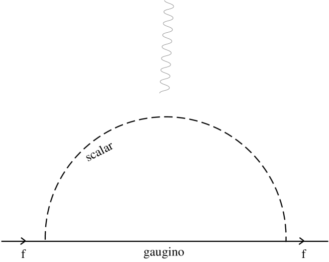
FIG. 1.: One loop diagram. The photon line can be attached to any charged particle.

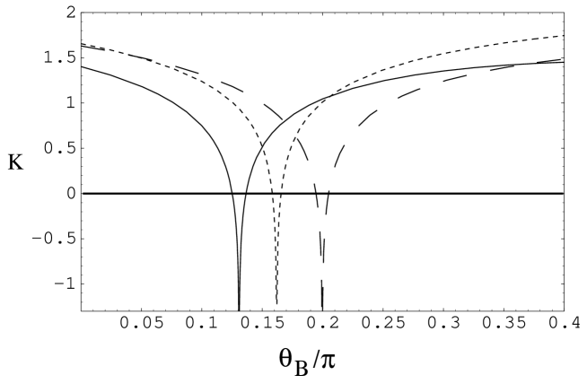
FIG. 2.: K vs. $\theta_{B}$ for $d_{e}$ for $m_{0}$=100 GeV, $m_{1/2}$=200 GeV, $|A_{0}|$=300 GeV, $\alpha_{0A}=\pi/2$, $\phi_{1}$=$\phi_{3}$=-1.1$\pi$(solid), -1.3$\pi$ (dashed), -1.5 $\pi$ (dotted) and tan$\beta$=3.

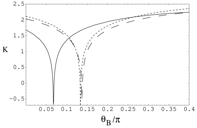
FIG. 3.: same as Fig.2 for tan$\beta$=10.

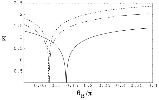
FIG. 4.: K vs. $\theta_{B}$ for $d_{e}$ for $\phi_{1}$=$\phi_{3}$=$\pi+\alpha_{0A}$=-1.25$\pi$, $m_{3/2}$=150 GeV, $\theta_{b}$=0.2, $\Theta_{1}=0.85$, with tan$\beta$=2(solid), 5(dashed), 10(dotted).

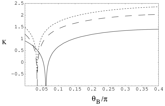
FIG. 5.: same as Fig.4 for $\phi_{1}$=$\phi_{3}$=$\pi+\alpha_{0A}$=-1.1$\pi$.

FIG. 6.: Central values of $\theta_{0B}$ for $d_{e}$ satisfying the EDM constraint as a function of tan$\beta$. Input parameters are as in Fig.4.

FIG. 7.: Values of $\Delta\theta_{0B}$ for $d_{e}$ satisfying the EDM constraint as a function of tan$\beta$. Input parameters are as in Fig.4.

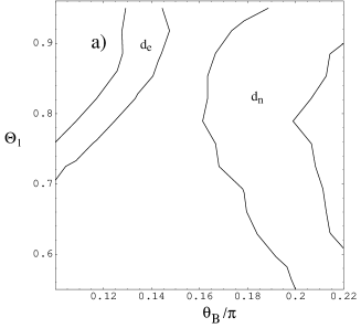
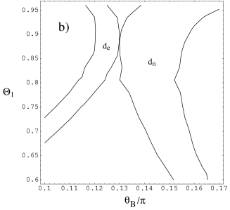
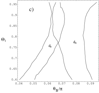
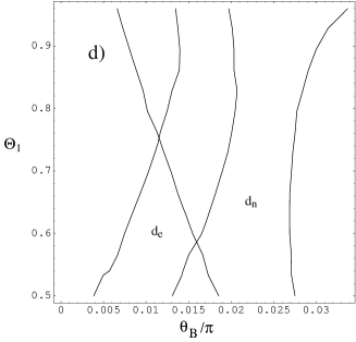
FIG. 8.: Allowed regions for $d_{e}$ and $d_{n}$ for tan$\beta$=2, $\theta_{b}$=0.2 and $m_{3/2}$=150 GeV. a) $\phi_{1}$=$\phi_{3}$=-1.25$\pi$, b) $\phi_{1}$=$\phi_{3}$=-1.60$\pi$, c) $\phi_{1}$=$\phi_{3}$=-1.80$\pi$ and d) $\phi_{1}$=$\phi_{3}$=-1.95$\pi$.

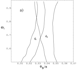
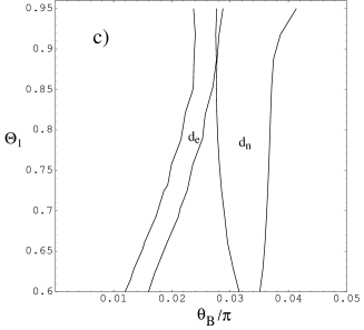
FIG. 9.: Allowed regions for $d_{e}$ and $d_{n}$ for $\theta_{b}$=0.2, $m_{3/2}$=150 GeV and $\phi_{1}$=$\phi_{3}$=-1.90$\pi$, for a) tan$\beta$=2, b) tan$\beta$=3 and c) tan$\beta$=5.

FIG. 10.: Allowed regions for $d_{e}$ and $d_{n}$ for $\theta_{b}$=0.2, $m_{3/2}$=150 GeV and $\phi_{1}$=$\phi_{3}$=-1.97$\pi$, for tan$\beta$=10.

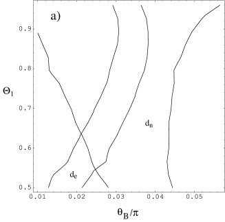
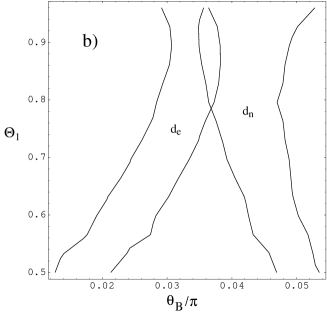
FIG. 11.: Allowed regions for $d_{e}$ and $d_{n}$ for $\theta_{b}$=0.2, $m_{3/2}$=150 GeV, tan$\beta=2$ and $\phi_{1}$=$\phi_{3}$=-1.90$\pi$ for a) $m_{u}$(1 GeV)=2.75 MeV, $m_{d}$(1 GeV)=5.0 MeV and b) $m_{u}$(1 GeV)=6.65 MeV, $m_{d}$(1 GeV)=12 MeV.

REFERENCES

• [1] J. Ellis, S. Ferrara and D.V. Nanopoulos, Phys. Lett. B114, 231 (1982); W. Buchmuller and D. Wyler, Phys. Lett. B121, 321 (1983); J. Polchinski and M.B. Wise, Phys. Lett. B125, 393 (1983).
• [2] E. Commins et al, Phys. Rev. A50 2960 (1994); K. Abdullah et al, Phys. Rev. Lett. 65, 2347 (1990); P. G. Harris et al, Phys. Rev. Lett. 82, 904 (1999).
• [3] T. Ibrahim and P. Nath, Phys. Lett. B418, 98 (1998).
• [4] M. Brhlik, G. Good, and G. Kane, Phys. Rev. D59, 115004 (1999).
• [5] S. Pokorski, J. Rosiek and C. A. Savoy, hep-ph/9906206.
• [6] T. Ibrahim and P. Nath, Phys. Rev. D57, 478 (1998); Erratum ibid. D58, 019901 (1998).
• [7] T. Ibrahim and P. Nath, Phys. Rev. D58, 111301 (1998).
• [8] T. Falk and K. Olive, Phys. Lett. B439, 71 (1998).
• [9] S. Barr and S. Khalil, hep-ph/9903425.
• [10] T. Falk , K. Olive, M. Pospelov and R. Roiban, hep-ph/9904393.
• [11] A. Bartl, T. Gajdosik, W. Porod, P. Stockinger and H. Stremnitzer, hep-ph/9903402.
• [12] E. Accomando, R. Arnowitt and B. Dutta, hep-ph/9907446.
• [13] M. Brhlik, L. Everett, G. Kane and J. Lykken, hep-ph/9905215.
• [14] Dai et al, Phys. Lett. B237, 216 (1990); Erratum, ibid B242, 547 (1990).
• [15] D. Chang, W-Y. Keung and A. Pilaftsis, Phys. Rev. Lett. 82, 900 (1999).
• [16] A. Manohar and H. Georgi, Nucl. Phys. B234, 189 (1984).
• [17] R. Arnowitt, J. L. Lopez, D.V. Nanopoulos, Phys. Rev. D42, 2423 (1990);R. Arnowitt, M. Duff and K. Stelle, Phys. Rev. D43, 3085 (1991).
• [18] D. Demir, Phys. Rev. D60, 055006 (1999). .
• [19] L.E. Ibanez and C. Lopez, Nucl. Phys. B233, 511 (1984); L.E. Ibanez, C. Lopez and C. Munoz, Nucl. Phys. B256, 218 (1985).
• [20] V. Barger, M. Berger and P. Ohmann, Phys. Rev. D49, 4908 (1994).
• [21] L. Ibanez, C. Munoz and S. Rigolin, Nucl. Phys. B553, 43 (1999).
• [22] G. Aldazabal, A. Font, L. Ibanez and G. Violero, Nucl. Phys. B536, 29 (1998).
• [23] A. Brignole, L. Ibanez, C. Munoz and C. Scheich, Z. Phys. C74, 157 (1997).
• [24] A. Brignole, L. Ibanez and C. Munoz, Nucl. Phys. B422, 125 (1994); Erratum ibid. B436, 747 (1995).
• [25] J. Gunion and H. Haber, Nucl. Phys. B272, 1 (1986); Erratum ibid. B402, 567 (1993).
• [26] The above results for tan$\beta$=2 are in general agreement with the corrected calculations of the results of Ref.[13].
• [27] H. Leutwyler, Phys. Lett. B374, 163 (1996).
• [28] M. Carena, S. Mrenna and C. Wagner, hep-ph/9907422.
Refer to caption