Power corrections and the interplay between perturbative and non-perturbative phenomena.

Abstract

We discuss the issue of interplay between perturbative and non-perturbative phenomena for power corrections to $e^{+}e^{-}$ event shapes.

1 Introduction

For some time now it has been known that to describe event-shape measures in $e^{+}e^{-}$ collisions, perturbative QCD on its own is not sufficient. In general there is a need for significant additional corrections, phenomenologically of the same size as the next-to-leading corrections, of non-perturbative (${\mathrm{NP}}$) origin. Initial estimates for these corrections came from Monte Carlo event generators [1, 2]. More recently, interest has arisen in analytic approaches [3, 4, 5, 6], based on ideas such as the high-order behaviour of perturbation theory (renormalons), or the concept of an infra-red-finite coupling, which predict corrections of order $1/Q$, where $Q$ is the centre-of-mass energy. This form is in rather good agreement with the experimentally required corrections, but there is no a priori method (except perhaps from the lattice) of determining the coefficient in front of $1/Q$: it is a fundamentally non-perturbative quantity. There is however the possibility that relative coefficients, from one observable to the next, may be estimated. This is referred to as the universality hypothesis.

As will be discussed in section 2, traditional methods for calculating the relative coefficients involve considering a $q\bar{q}$ pair together with a single soft gluon. It turns out that event shapes can be divided into two categories according to their behaviour in the presence of a $q\bar{q}$ pair and many soft gluons: those whose value is a linear combination of contributions from each of the soft gluons, and those which instead involve a non-linear combination. The traditional methods are adequate for linear observables. But they are not suitable for non-linear ones because the presence of perturbative ($\mathrm{PT}$) soft gluons requires that one take into account correlations between $\mathrm{PT}$ and ${\mathrm{NP}}$ gluons. Section 3 illustrates how this is done.

1.1 Event-shape definitions

Let us first define the event-shapes that will be considered here. The thrust is given by,

$$T=\max_{{\vec{n}}}\frac{\sum_{i}|{\vec{k}}_{i}.{\vec{n}}|}{\sum_{i}|{\vec{k}}_{i}|}\,,$$ (1)

and measures the extent to which an event is ‘pencil-like’. The $C$-parameter is

$$C=\frac{3}{2}\sum_{ij}k_{i}k_{j}\sin^{2}\theta_{ij}\>.$$ (2)

The heavy jet mass is,

$$\rho_{h}=\frac{M_{h}^{2}}{Q^{2}}\,,$$ (3)

where $M_{h}^{2}$ is the invariant mass of the heavier of the two hemispheres defined by a plane perpendicular to the thrust axis ${\vec{n}}$. Finally we have the total jet-broadening,

$$B_{T}=\frac{1}{2Q}\sum_{i}|k_{t,i}|\,,$$ (4)

where the $k_{t}$ are measured perpendicular to the thrust axis. A similar quantity, known as the wide-jet broadening, $B_{W}$, is defined as the larger of the broadenings calculated separately in the two hemispheres.

These events shapes have the property that in the limit of a two-jet event, $1-T$, $C$, $\rho_{h}$, $B_{T}$ and $B_{W}$ go to zero.

2 Traditional power corrections

There are many related approaches to the calculation of power corrections to event shapes (and to a whole range of other observables): renormalons [3], the massive gluon approach [4], the dispersive approach [5], the two-loop approach [6]. In event-shape studies, they essentially reduce to considering the behaviour of the observable in the presence of the $q\bar{q}$ pair and a single soft gluon. For a soft gluon with transverse momentum $k_{t}$ and rapidity $\eta$, the value of the event shape variable $V$ is given by $k_{t}/Q$ times a ‘characteristic function’ $f_{V}(\eta)$:

$V=$	$1-T$	$C$	$\rho_{h}$	$B_{T}$	$B_{W}$
$f_{V}=$	$e^{-|\eta|}$	$\frac{3}{\cosh\eta}$	$e^{-|\eta|}$	$1$	$1$

plus terms of order $k_{t}^{2}/Q^{2}$. Schematically, the power correction can be seen as coming from the integral of this characteristic function over rapidity and transverse momentum, including a factor of $\alpha_{\mathrm{s}}(k_{t})$.

More specifically, one considers only the non-perturbative part of $\alpha_{\mathrm{s}}$, (which we’ll call $\alpha_{\mathrm{NP}}$), which is non-zero only for small scales of the order of a GeV. So we have an expression for the power correction which is

$$\delta V=\frac{2C_{F}}{\pi}\int\frac{{\mathrm{d}}k_{t}}{k_{t}}\,\frac{k_{t}}{Q}\,\alpha_{{\mathrm{NP}}}(k_{t})\int{\mathrm{d}}\eta\,f_{V}(\eta)\,.$$ (5)

Since all the observables have the same dependence on $k_{t}$, the integral over $k_{t}$ yields the same value in each case:

$$\!\!\!\!\!\!\!\!\!\!\!\!\int\frac{dk_{t}}{k_{t}}\frac{k_{t}}{Q}\alpha_{{\mathrm{NP}}}(k_{t}) =\int^{\mu_{I}}\!dk_{t}\,\frac{\alpha_{\mathrm{s}}(k_{t})-\alpha_{\mathrm{PT}}(k_{t})}{Q}$$

$$=\alpha_{0}(\mu_{I})\frac{\mu_{I}}{Q}+{\cal O}\left({\alpha_{\mathrm{s}}(Q)\frac{\mu_{I}}{Q}}\right),$$ (6)

where $\alpha_{\mathrm{PT}}$ is the perturbative expansion for $\alpha_{\mathrm{s}}$ around scale $Q$; the integral can be truncated at $\mu_{I}\sim 2$ GeV, because beyond that scale $\alpha_{{\mathrm{NP}}}$ should die off very quickly.

The observable-dependent part of the power correction comes from the integral over rapidity, which yields an observable-dependent coefficient, $c_{V}$,

$$c_{V}=\int{\mathrm{d}}\eta\,f_{V}(\eta)\,,$$ (7)

multiplying $\alpha_{0}/Q$.

The postulate that $\alpha_{0}$ experimentally really is the same for all variables, is referred to as universality. A priori we have no way of calculating $\alpha_{0}$ (except perhaps on the lattice [8]), but we should be able to measure it in different observables and find it to be consistently the same.

3 Interplay with the perturbative event

The power correction as calculated above is valid for a situation in which the non-perturbative gluon which we consider (termed ‘gluer’ by Dokshitzer [9]) is the only particle present apart from the initial $q\bar{q}$ pair. In practice however the event nearly always contains many soft and collinear gluons of perturbative origin. There could also be several ‘gluers’.

So we need to understand what happens to the event shape in the presence of more than one soft particle.

3.1 The thrust and $C$-parameter

Some variables, such as the thrust are simple. In the presence of many soft particles, $1-T$ just becomes

$$1-T\simeq\sum_{i}\frac{k_{t,i}}{Q}e^{-|\eta_{i}|}\,,$$ (8)

i.e. it is a linear combination of the contributions from each soft particle. Thus the contribution of the gluer will just add to that of the underlying perturbative event, and the consideration of the power correction based on the presence of just a single gluon will remain valid. A similar argument applies to the $C$-parameter.

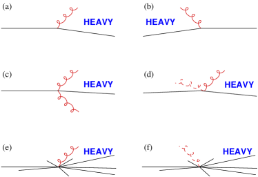
Figure 1: Situations of relevance for the heavy-jet mass. Solid straight lines represent the underlying perturbative event. Curly lines are gluers. Dashed gluers do not contribute to the heavy-jet mass.

3.2 The heavy-jet mass

Considering the heavy-jet mass $\rho_{h}$, we find that the situation is somewhat different. As given above, in the presence of a single gluon (figs. 1a and 1b), $\rho_{h}$ is just $k_{t}/Qe^{-|\eta|}$, because the heavy-jet is always the one containing the gluon. In the presence of two particles in the same hemisphere (fig. 1c), then the contribution is

$$\frac{1}{Q}\left(k_{t,1}e^{-|\eta_{1}|}+k_{t,2}e^{-|\eta_{2}|}\right)\,,$$ (9)

which is fine because it is a linear combination of the two contributions. But when the two gluons are in opposite hemispheres (fig. 1d), the heavy jet mass is the larger of the two hemisphere masses:

$$\frac{1}{Q}\max\left(k_{t,1}e^{-|\eta_{1}|},k_{t,2}e^{-|\eta_{2}|}\right)\,,$$ (10)

This is a non-linear combination of the two contributions, which means that in the presence of the full $\mathrm{PT}$ event, the power correction cannot simply be estimated by adding the 1-gluon result to the perturbative answer.

So how do we determine the power correction in this case? The fundamental point is to observe that the contribution to the event shape from the underlying perturbative event is always much larger than that from the gluers. To see why, consider that because of Sudakov suppression of events without soft and collinear gluons, the probability of an event-shape variable $V$ being smaller than some value $V_{\max}\ll 1$ is roughly

$$P(V<V_{\max})\sim\exp\left(-N\frac{\alpha_{\mathrm{s}}C_{F}}{2\pi}\ln^{2}V_{\max}\right)$$ (11)

where $N$ is a variable-dependent number. Thus typical values for $V$ are of the order of

$$V_{\mathrm{typical}}\sim\exp\left(-\frac{1}{\sqrt{\alpha_{\mathrm{s}}}}\right)\sim\exp\left(-\sqrt{\ln Q}\right)\,.$$

The contribution from non-perturbative effects,

$$V_{{\mathrm{NP}}}\sim\frac{1}{Q}\sim\exp\left(-\ln Q\right)\,,$$

is much smaller.

As a result, in the limit of large $Q$, it will be the perturbative event which ‘decides’ which hemisphere is heavy (figs. 1e and 1f). Once that information is known, $\rho_{h}$ is just a linear combination of the contributions from all the particles in the heavier hemisphere. So by invoking the large difference between the typical perturbative and non-perturbative scales, we have been able to reduce the heavy-jet mass to being linear in the contributions from the gluers. Since it is only gluers in one of the hemispheres that are relevant, we halve the power correction compared to the single gluon estimate [10, 7].

3.3 The jet broadenings

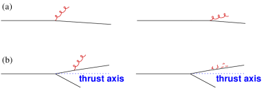
Figure 2: Broadening for different quark axes.

The jet-broadenings give a particularly rich example of a non-linear event-shape observable which is reduced to being linear in the presence of perturbative radiation.

In the presence of a single soft gluon there is a contribution from the transverse momentum of the gluon and from the recoil momentum of the quark. Noting the factor of a half in the definition of the broadening, eq. (4), one obtains that the contribution to B is $k_{t}/Q$. In the presence of two soft gluons in the same hemisphere, the situation becomes more complex: the contributions to $B$ from the $k_{t}$’s of the soft gluons will simply be $(k_{t,1}+k_{t,2})/2Q$; but the contribution from the quark recoil will be $|{\vec{k}}_{t,1}+{\vec{k}}_{t,2}|/2Q$, which is anything but simple, especially if one starts having to take into account many gluons. This first complication is resolved by noting that recoil from perturbative radiation will cause the quark to have a large (relative to the ${\mathrm{NP}}$ scale) transverse momentum $p_{t}$. After carrying out the integration over the azimuthal angle of the gluer one obtains that the recoil due to the gluer is

$$\!\!\!\!\!\!\!\!\!\!\!\!\!\int_{0}^{2\pi}\frac{d\phi}{2\pi}\left(\sqrt{p_{t}^{2}+k_{t}^{2}+2k_{t}p_{t}\cos\phi}-p_{t}\right)\simeq\frac{k_{t}^{2}}{4p_{t}}$$ (12)

Being quadratic in $k_{t}$, this will lead at most to a $1/Q^{2}$ correction. So in the presence of $\mathrm{PT}$ radiation we can neglect quark recoil. This halves one’s expectation for the power correction (since in the 1-gluon approximation equal contributions came the gluon and from the quark recoil), but still leaves it proportional to $(\ln Q/\Lambda)/Q$. This form arises because the integral over rapidity, (7) is bounded by the kinematic limit which is approximately $\ln Q/k_{t}\simeq\ln Q/\Lambda$. Experimentally, this was found by both the H1 and JADE collaborations to be incompatible with the data [11, 12]. The JADE collaboration made the additional observation that the power correction seemed to depend on the value of $B$ itself.

The further element that has been neglected is that of the axis with respect to which one measures the transverse momenta. One assumes a $dk_{t}/k_{t}$ distribution for emission, where $k_{t}$ is given with respect to the quark axis, but the broadening measures transverse momenta with respect to the thrust axis. The extent to which these two axes coincide affects the power correction. This is illustrated in figure 2. If the quark axis and thrust axis coincide, fig. 2a, then gluons with (the same $k_{t}$ and) large and small angles to the quark axis contribute equally. If on the other hand the quark axis does not coincide with the thrust axis, fig. 2b, then gluons at large angles to the quark axis contribute as before. But gluons close to the quark axis (angles smaller than the angle between the thrust and quark axes) do not contribute — or more precisely their contribution is exactly cancelled by a corresponding longitudinal recoil of the quark. Therefore the rapidity integral for the gluer does not extend beyond the quark rapidity, $\eta_{q}$, leading to a power correction proportional to $\eta_{q}/Q$. To determine $\eta_{q}$, one observes that it is determined by the hardest gluon (transverse momentum $p_{t}$) in the event, so that $\eta_{q}\simeq\ln Q/p_{t}\simeq\ln 1/B$. Thus we arrive at the result that (for a single hemisphere — $B_{1}$), the coefficient of the power correction is [13]

Figure 3: Fit to the mean jet-broadening, using a power correction of the form (15). The lowest line is the LO prediction, the next line includes the NLO corrections, and the highest line includes additionally the power correction.

$$c_{B_{1}}(B_{1})=\frac{1}{2}\ln\frac{1}{B_{1}}+{\cal O}\left({1}\right)\,.$$ (13)

This applies separately for the broadenings from each hemisphere.

Mean Broadenings

Let us first use this information to determine the power correction to the mean broadenings. We have to integrate the power correction with the perturbative distribution for the broadening. This has to be done separately for each hemisphere. The perturbative distribution for the single-hemisphere broadening goes roughly as

$$\!\!\!\!\!\!\!\!\!\!\frac{B_{1}}{\sigma}\frac{{\mathrm{d}}\sigma}{{\mathrm{d}}B_{1}}\simeq\frac{2\alpha_{\mathrm{s}}C_{F}}{\pi}\ln\frac{1}{B_{1}}\exp\left(-\frac{\alpha_{\mathrm{s}}C_{F}}{\pi}\ln^{2}B_{1}\right)$$ (14)

Integrating this with (13) and including a factor of two to take into account the two hemispheres gives us the coefficient of the power correction for the broadening:

$$\langle c_{B_{T}}\rangle=\frac{\pi}{\sqrt{\alpha_{\mathrm{s}}C_{F}}}+{\cal O}\left({1}\right)\,,$$ (15)

where the terms of ${\cal O}\left({1}\right)$ are to be found in [13]. This form for the power correction is used in figure 3 where one sees good agreement with the data.

For the wide-jet broadening, the distribution is similar to (14) but with an extra factor of two in front of each $\alpha_{\mathrm{s}}$. This together with the the fact that we have the ${\mathrm{NP}}$ contribution from just one hemisphere, gives a power correction coefficient of

$$\langle c_{B_{W}}\rangle=\frac{\pi}{2\sqrt{2\alpha_{\mathrm{s}}C_{F}}}+{\cal O}\left({1}\right)\,.$$ (16)

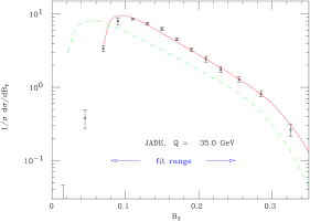
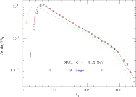
Figure 4: The distribution of the total jet-broadening from the JADE [12] and OPAL [14] collaborations, compared to theoretical predictions: the dashed lines are the resummed perturbative prediction, while the solid lines include the power correction. The parameters, $\alpha_{\mathrm{s}}=0.1158$ and $\alpha_{0}=0.5368$, have been obtained from a fit to $B_{T}$ distributions at a range of energies.

Broadening distributions

The situation for the distribution of the total jet-broadening is a little trickier. Essentially, for small jet-broadenings each hemisphere contains about half the total broadening and the power correction is roughly twice (13):

$$c_{B_{T}}(B_{T})\simeq\ln\frac{2}{B_{T}}+{\cal O}\left({1}\right)\,.$$ (17)

For larger jet-broadenings, most of the jet-broadening comes from one hemisphere (whose power correction is just (13)), while the other hemisphere is essentially free to have almost any value of the broadening and so its power correction is half of (15) giving a total of

$$c_{B_{T}}(B_{T})\simeq\frac{1}{2}\ln\frac{1}{B_{T}}+\frac{\pi}{2\sqrt{\alpha_{\mathrm{s}}C_{F}}}+{\cal O}\left({1}\right)\,.$$ (18)

Again, the full formulae, which interpolate between the two regimes, are given in [13]. Two examples of the broadening distribution compared to data are shown in figure 4 and the need for and success of the power correction are clearly visible.

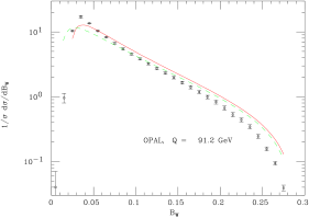
Figure 5: The distribution of the wide-jet broadening: a comparison of OPAL data [14] and the resummed distribution, with (solid line) and without (dashed line) the power correction. The parameters used are those obtained from the fit to the $B_{T}$ distribution, c.f. figure 4. (The best fit parameters for the $B_{W}$ distribution are quite different, and are shown in figure 6).

The power correction to the distribution of the wide-jet broadening is much simpler since we only have one hemisphere to worry about. It is given simply by (13). The comparison to the data is however quite unsatisfactory. The distribution is shown together with OPAL data [14] in figure 5. There is quite clear disagreement, with a substantial need for the whole distribution to be squeezed to smaller $B_{W}$, especially at moderate and large values of $B_{W}$. Currently the origin of this problem is not understood. But it should be noted that the wide-jet broadening is in some respects quite a subtle variable: for example, going from a three-jet to a four-jet event can reduce the value of $B_{W}$. These subtleties may translate into large higher-order corrections, both to the perturbative and non-perturbative parts.

Figure 6: 2-$\sigma$ contours for fit results to various observables. No theoretical systematic errors are taken into account. Solid lines indicate fits to distributions, while dashed lines indicate fits to mean values. The solid curves for $C$ and $T$ are the results of fits carried out by the JADE collaboration [12].

4 Conclusions

Figure 6 shows 2-$\sigma$ contours from fits to a variety of observables, both for distributions and mean values. Given that one does not necessarily expect $\alpha_{0}$ to be consistent between one observable and another to better than $20\%$, because of potential higher-order non-perturbative effects, and that theoretical systematic errors have not been taken into account, the agreement for $\alpha_{\mathrm{s}}$ and $\alpha_{0}$ between observables is fairly reasonable. The only exception is the wide-jet broadening, which as we have seen above has yet to be fully understood.

Thus the approach of power corrections is a powerful tool in the analysis of event shapes. An important element in its success is a treatment of the interplay between perturbative and non-perturbative radiation.

References

- [1] G. Marchesini, B.R. Webber, G. Abbiendi, I.G. Knowles, M.H. Seymour and L. Stanco, Comput. Phys. Commun. 67 (1992) 465.
- [2] T. Sjostrand, Comput. Phys. Commun. 82 (1994) 74.
- [3] A.V. Manohar and M.B. Wise, Phys. Lett. B 344 (1995) 407 [hep-ph/9406392]; G.P. Korchemsky and G. Sterman, Nucl. Phys. B 437 (1995) 415 [hep-ph/9411211]; R. Akhoury and V.I. Zakharov, Phys. Lett. B 357 (1995) 646 [hep-ph/9504248].
- [4] Yu.L. Dokshitzer and B.R. Webber, Phys. Lett. B 352 (1995) 451.
- [5] M. Beneke and V.M. Braun, Phys. Lett. B 348 (1995) 513 [hep-ph/9411229] ; P. Ball, M. Beneke and V.M. Braun, Nucl. Phys. B 452 (1995) 563 [hep-ph/9502300] ; Yu.L. Dokshitzer, G. Marchesini and B.R. Webber, Nucl. Phys. B 469 (1996) 93 [9512336].
- [6] Yu.L. Dokshitzer, A. Lucenti, G. Marchesini and G.P. Salam, Nucl. Phys. B 511 (1998) 396 [hep-ph/9707532].
- [7] Yu.L. Dokshitzer, A. Lucenti, G. Marchesini and G.P. Salam, JHEP 05 (1998) 003 [hep-ph/9802381].
- [8] G. Burgio, F. Di Renzo, C. Parrinello and C. Pittori, hep-ph/9808258.
- [9] Yu.L. Dokshitzer, V.A. Khoze, A.H. Mueller and S.I. Troyan, Basics of Perturbative QCD, ed. J. Tran Thanh Van, Editions Frontières, Gif-sur-Yvette, 1991.
- [10] R. Akhoury and V.I. Zakharov, Nucl. Phys. B 465 (1996) 295 [hep-ph/9507253].
- [11] H1 Collaboration, C. Adloff et al., Phys. Lett. B 406 (1997) 256 [hep-ex/9706002]; contribution 530 to ICHEP July 1998, Vancouver, Canada.
-
[12]
P.A. Movilla Fernández, talk at QCD Euroconference,
Montpellier, France, July 1998,
hep-ex/9808005;
P.A. Movilla Fernández, O. Biebel and S. Bethke, paper contributed to ICHEP-98, Vancouver, Canada, hep-ex/9807007. - [13] Yu.L. Dokshitzer, G. Marchesini and G.P. Salam, Eur. Phys. J. Direct C 3 (1999) 1 [hep-ph/9812487].
- [14] OPAL Collaboration, P.D. Acton et al., Z. Physik C 59 (1993) 1;