Figure 1

Figure 2

Figure 3

Figure 4

IPNO-DR 99-22

$N_{f}$ DEPENDENCE OF THE QUARK CONDENSATE
FROM A CHIRAL SUM RULE

Bachir Moussallam

I.P.N., Groupe de Physique Théorique
Université Paris-Sud, F-91406 Orsay Cédex

Abstract

How fast does the quark condensate in QCD-like theories vary as a function of $N_{f}$ is inferred from real QCD using chiral perturbation theory at order one-loop. A sum rule is derived for the single relevant chiral coupling-constant, $L_{6}$. A model independent lower bound is obtained. The spectral function satisfies a Weinberg-type superconvergence relation. It is discussed how this, together with chiral constraints allows a solid evaluation of $L_{6}$, based on experimental $\pi\pi-K\bar{K}$ S-wave T-matrix input. The resulting value of $L_{6}$ is compatible with a strong $N_{f}$ dependence possibly suggestive of the proximity of a chiral phase transition.

1 Introduction

By analogy with recent results obtained in supersymmetric theories[1], one expects that QCD-like theories will undergo a number of phase transitions at zero temperature upon varying $N_{f}$, the number of different flavour fermions, at fixed number of colours ($N_{c}=3$ in the following). If the number of fermions is large $N_{f}>{11\over 2}N_{c}$ the theory has no asymptotic freedom and no confinement. Decreasing $N_{f}$ below ${11\over 2}N_{c}$ one encounters a conformal phase as indicated by the fact that the $\beta$-function at two loops has a zero[2]. Assuming the fermions to be all massless, the chiral $SU(N_{f})\times SU(N_{f})$ symmetry of the QCD action remains unbroken in this phase. If one further decreases $N_{f}$ to small values, $N_{f}=2-3$, then QCD is in a confining phase in which the chiral group is spontaneously broken to $SU(N_{f})$. It is generally believed that, in this phase, the quark condensate is non-vanishing and large. At larger $N_{f}$, there could exist different phases of chiral symmetry breaking. A physical picture of such phases is proposed in ref.[4]. An interesting open question concerns the value of $N_{f}^{crit}$ for which a chiral phase transition takes place. Recent lattice results suggest that a transition could occur for $N_{f}$ as small as four[5]. In an instanton vacuum model, the quark condensate ceases to be non-vanishing for $N_{f}$ of the order of five[6], while another theoretical model obtains a much larger value[7].

In this paper, we use the fact that nature solves ordinary QCD in order to extract an information on how the quark condensate varies with $N_{f}$ for small values of $N_{f}$. More specifically, if it can be shown that the ratio

$$R_{32}={<{\bar{u}u}>_{N_{f}=3}\over<{\bar{u}u}>_{N_{f}=2}}$$ (1)

is significantly smaller than one, one may expect a rather small value of $N_{f}^{crit.}$. In the functional integral, the dependence upon $N_{f}$ arises from the fermion determinant part of the measure: setting all quark masses equal, one has

$$d\mu\equiv d\mu(A)\left(\det(i\mathrel{\hbox{$D$}\kern-6.41771pt\hbox{$/$}}+m)\right)^{N_{f}}\ .$$ (2)

In other terms, it is a Dirac sea effect. In the quenched approximation, which is often used in lattice simulations, the fermion determinant is set equal to one and $R_{32}$ is exactly one. The same result also follows in the leading large $N_{c}$ expansion of QCD, since the determinant contributes to graphs with internal quark loops, which are subleading. Using chiral perturbation theory (CHPT), one can access the ratio

$$\tilde{R}_{32}={<{\bar{u}u}>_{(m_{u}=m_{d}=m_{s}=0)}\over<{\bar{u}u}>_{(m_{u}=m_{d}=0,m_{s}\neq 0)}}\ .$$ (3)

This ratio is different from $R_{32}$, but it is also a measure of the influence of the fermion determinant in the evaluation of the quark condensate. Again, this ratio would be exactly one in the leading large $N_{c}$ expansion or in the quenched approximation, for any value of the strange quark mass $m_{s}$. The point here is that the physical value of strange quark mass is sufficiently small compared to the scale of the chiral expansion $\Lambda\sim 1$ GeV, such that the chiral expansion in $m_{s}/\Lambda$ makes sense and, at the same time, $m_{s}$ is not that small so that $\tilde{R}_{32}$ will not trivially be close to one. In this paper, we will provide an estimate of $\tilde{R}_{32}$.

The plan of the paper is as follows. In sec.2, the expression of $\tilde{R}_{32}$ in CHPT at order one-loop is given. This expression involves a single low-energy coupling constant, $L_{6}(\mu)$, in the nomenclature of Gasser and Leutwyler[9]. In that paper, $L_{6}$ was simply assumed to be OZI suppressed. Here, we attempt a more careful estimate on the basis of a chiral sum rule. Analogous chiral sum rules were discussed in the recent literature[10] and eventually provide very good precision[11]. In sec.3, a sum rule expression for $L_{6}$ in terms of the correlation function $\Pi_{6}(s)$ of two scalar currents $\bar{u}u+\bar{d}d$ and $\bar{s}s$ is established and $Im\Pi_{6}(s)$ is shown to satisfy a Weinberg-type sum rule. This will be an important constraint to our evaluation. The construction of the spectral function is discussed in sec.4. Important ingredients are the pion and the kaon scalar form-factors which can be related to experimental information on pion-pion scattering using analyticity, unitarity, high-energy constraints as well as low-energy constraints from chiral symmetry. This was first performed in ref.[12]. Extension to the region of 1.5 GeV, where important resonance contribution is expected is then discussed. Finally, the result can be found in sec.6.

2. Ratio of quark condensates from CHPT

Consider QCD in a limit where $N_{f}$ quarks are exactly massless. We will consider the cases of $N_{f}=2$ and $N_{f}=3$ and assume, a priori, that chiral symmetry is spontaneously broken in QCD in both cases and that the value of the condensate is sufficiently large also in both cases such that the conventional chiral expansion [13][9] applies. In nature, none of the quark masses $m_{u}$, $m_{d}$ $m_{s}$ is exactly vanishing, but they are in an asymmetric configuration where $m_{u},\ m_{d}<<m_{s}$ (by a factor of twenty or so) and $m_{s}$ is itself sufficiently small compared to the scale of the chiral expansion $\Lambda$. Using this fact, one can express the ratio $\tilde{R}_{32}$ as an expansion in powers of $m_{s}$. At chiral order $O(p^{4})$, making use of the formulae of ref.[9], one obtains

$$\tilde{R}_{32}=1-{m_{s}B_{0}\over{F_{\pi}}^{2}}\left[32L_{6}(\mu)-{1\over 16\pi^{2}}\left({11\over 9}\ln{m_{s}B_{0}\over\mu^{2}}+{2\over 9}\ln{4\over 3}\right)\right]+O(m^{2}_{s})\ ,$$ (4)

At order $O(p^{2})$ one has,

$$m_{s}B_{0}={1\over 2}\left(M^{2}_{K^{+}}+M^{2}_{K^{0}}-M^{2}_{\pi^{+}}\right),$$ (5)

and this value can be used consistently in the equation above. The size of $\tilde{R}_{32}$ depends on the value of a single low-energy coupling constant, $L_{6}$.

The low-energy coupling constants of CHPT may be related to QCD correlation functions evaluated near zero momenta. This can be exploited, in particular for two-point functions, in order to express these constants in the form of sum rules using analyticity (and the fact that chiral correlators have non-singular short distance behaviour). A number of these are exhibited in ref.[13]. A classic example concerns the coupling constant $L_{10}$ which is related to the correlation function of two vector currents minus two axial currents. A very reasonable estimate for $L_{10}$ can be obtained using simply the idea of vector meson dominance as well as Weinberg sum rules[14]. Our aim is to estimate $L_{6}$ along similar guidelines.

One specific reason for interest in $L_{6}$ is in connection with the Kaplan-Manohar transformation[15]. These authors observed that the effective lagrangian is left invariant under the following transformation of the quark mass matrix,

$${\cal M}\to{\cal M}+\alpha\left(32B_{0}\over F^{2}_{\pi}\right)({\cal M^{\dagger}})^{-1}\det{\cal M},$$ (6)

together with a transformation of certain low-energy constants. At chiral order $O(p^{4})$ three coupling constants are affected, $L_{6}$, $L_{7}$ and $L_{8}$, which get transformed as

$$L_{6}\to L_{6}-\alpha,\quad L_{7}\to L_{7}-\alpha,\quad L_{8}\to L_{8}+2\alpha\ .$$ (7)

One consequence is that using low-energy data alone, one can only determine combinations which are invariant under this transformation and not the individual values of $L_{6}$, $L_{7}$ and $L_{8}$. These values are of some importance. In particular, the value of $L_{8}$ determines the ratio of quark masses $2m_{s}/(m_{u}+m_{d})$ beyond the leading chiral order[9]. It is therefore of interest to explore means of separately determining these constants (or at least one of them).

3. Sum rule for $L_{6}$

Consider the correlation function of the two scalar, isoscalar currents $\bar{u}u+\bar{d}d$ and $\bar{s}s$,

$$\Pi_{6}(p^{2})=iB_{0}^{-2}\int d^{4}xe^{ipx}<T\left[(\bar{u}u(x)+\bar{d}d(x))\,\bar{s}s(0)\right]>_{c},$$ (8)

where the subscript $c$ means that only connected graphs are to be retained. The factor $B_{0}^{-2}$ is introduced to simplify forthcoming expressions and furthermore makes $\Pi_{6}$ a renormalisation scale invariant object and $B_{0}$ is defined as

$$B_{0}=-\lim_{m_{u}=m_{d}=m_{s}=0}{<\bar{u}u>\over F^{2}_{\pi}}\ .$$ (9)

For small momenta we can express $\Pi_{6}(p^{2})$ using CHPT. In particular, at zero momentum, from CHPT at $O(p^{4})$ one obtains,

$$\Pi_{6}(0)=64L_{6}(\mu)-{1\over 16\pi^{2}}\left[2\ln{(m_{s}+m)B_{0}\over\mu^{2}}+{4\over 9}\ln{(4m_{s}+2m)B_{0}\over 3\mu^{2}}+{22\over 9}\right]+O(m,m_{s}).$$ (10)

Here, and in the following, isospin breaking is neglected and we set $m_{u}=m_{d}=m$. This expression is at the basis of our sum rule estimate for $L_{6}$. The quark condensate ratio $\tilde{R}_{32}$ has a very simple expression in terms of $\Pi_{6}$. Combining equations (4) and (10) one obtains

$$\tilde{R}_{32}=1-{{\bar{M}_{K}}^{2}\over 32\pi^{2}\bar{F}^{2}_{\pi}}\left[16\pi^{2}\bar{\Pi}_{6}(0)+{22\over 9}\right]+O(m^{2}_{s}),$$ (11)

where barred quantities are to be taken in the limit $m_{u}=m_{d}=0$. This relation (and eq.(4)) can be recovered alternatively by noting that

$${\partial\over\partial m_{s}}<\bar{u}u+\bar{d}d>=-B^{2}_{0}\Pi_{6}(0),$$ (12)

and integrating this equation from $m_{s}=0$ to its physical value using the CHPT expression (10).

It is possible to derive a lower bound on $L_{6}$ and on $\bar{\Pi}_{6}(0)$ based on general properties of the QCD measure. At first, it is not very difficult to show that $\Pi_{6}(0)$ must be positive in the case of equal quark masses [16]. Let $Z$ be the partition function of euclidian QCD,

$$Z=\int d\mu(A)\,e^{-S_{YM}(A)}{\rm det}(i\mathrel{\hbox{$D$}\kern-6.41771pt\hbox{$/$}}_{A}+M),\quad M=diag(m,m,m_{s})\ .$$ (13)

We can express $\Pi_{6}(0)$ in terms of $Z$ as

$$\Pi_{6}(0)={1\over Z}{d^{2}Z\over dmdm_{s}}-{1\over Z}{dZ\over dm}\,{1\over Z}{dZ\over dm_{s}}\ .$$ (14)

In the limit $m_{s}=m$ this can be written as an average of a manifestly positive quantity,

$$\lim_{m_{s}=m}\Pi_{6}(0)=<\left({\rm Tr}{1\over i\mathrel{\hbox{$D$}\kern-6.41771pt\hbox{$/$}}+m}-<{\rm Tr}{1\over i\mathrel{\hbox{$D$}\kern-6.41771pt\hbox{$/$}}+m}>\right)^{2}>\ ,$$ (15)

where averages are defined as

$$<O>={1\over Z}\int d\mu(A)\,e^{-S_{YM}(A)}{\rm det}(i\mathrel{\hbox{$D$}\kern-6.41771pt\hbox{$/$}}_{A}+M)O(A)\ .$$ (16)

This is because ${\rm Tr}\,{(i\mathrel{\hbox{$D$}\kern-6.41771pt\hbox{$/$}}+m)^{-1}}$ can be shown to be real and the averaging is performed with respect to an integration measure which is real and positive in euclidian QCD (assuming the vacuum angle $\theta=0$ and a proper regularisation of the fermion determinant). We can now apply this result on the positivity of $\Pi_{6}(0)$ in conjunction with its one-loop expression, eq.(10), setting all three quark masses there equal to the physical $m_{s}$ value. One gets

$$L_{6}(\mu)\geq{11\over 4608\pi^{2}}\left[\log{2m_{s}B_{0}\over\mu^{2}}+1\right]+O(m_{s})\ .$$ (17)

Ignoring higher loop corrections, this gives

$$10^{3}L_{6}(M_{\eta})\geq 0.35,\quad 16\pi^{2}\bar{\Pi}_{6}(0)\geq 1.57\ .$$ (18)

This shows, in particular, that the condensate must be a decreasing function of $N_{f}$.

Another property, which will prove an important constraint for the sum rule estimate of $L_{6}$ is that $\bar{\Pi}_{6}$ satisfies a Weinberg-type sum rule (WSR)

$$\int_{0}^{\infty}Im\bar{\Pi}_{6}(s)ds=0\ .$$ (19)

The proof is analogous to that of the ordinary Weinberg sum rules (see e.g. [17] ). The operators in the operator-product expansion at short distances must transform in the same way as $(\bar{u}u+\bar{d}d)\,\bar{s}s$ under the chiral group. The masses $m_{u}$ and $m_{d}$ being set equal to zero, the operator of lowest dimensionality having the correct transformation property is $m_{s}(\bar{u}u+\bar{d}d)$ and it has dimension four. Furthermore, a factor of $(\alpha_{s})^{2}$ is generated from the fact that all connected graphs contain at least two gluon lines. Taking into account the scale dependence of $\alpha_{s}$ and that of $B_{0}$ in the perturbative region, we learn that $\bar{\Pi}_{6}$ vanishes asymptotically faster than $1/q^{2}$,

$$\bar{\Pi}_{6}(q^{2})={C<m_{s}(\bar{u}u+\bar{d}d)>\over q^{2}\left[\ln(-q^{2})\right]^{2+24/27}}+O({1\over q^{4}}),$$ (20)

with $C$ a constant, which implies the WSR eq.(19). Furthermore, this behaviour ensures convergence of an unsubtracted dispersion relation for $\bar{\Pi}_{6}$, so that one can express its value at zero as

$$\bar{\Pi}_{6}(0)={1\over\pi}\int_{0}^{\infty}ds\,{Im\bar{\Pi}_{6}(s)\over s}\ .$$ (21)

While the WSR must be satisfied for arbitrary values of $m_{s}$, it is clear from eq.(20) that convergence of the integral (19) will be faster if $m_{s}=0$. In that situation, one expects the sum rule to be saturated in an energy interval of, say, $[0-2]$ GeV, by analogy with the ordinary Weinberg sum rules. Experimental data is known for $m_{s}\neq 0$, but while there may be large differences locally in $Im\Pi_{6}(s)$ upon varying the value of $m_{s}$ (notably because of threshold effects), it is expected that these differences will be smoothed out to a large extent in the integral. One therefore expects that the WSR will be also approximately saturated in a finite energy region, for the physical value of $m_{s}$.

Let us make some qualitative remarks on the practical significance of the sum rule. In the large $N_{c}$ counting, $\Pi_{6}$ is suppressed compared to a generic QCD correlation function, it is of order $O((N_{c})^{0})$ instead of $O(N_{c})$. As a byproduct, one observes that the contribution of a single resonance is not enhanced by a factor of $N_{c}$ compared to the non-resonant background. In the large $N_{c}$ world, the coupling of a resonance to either $\bar{u}u+\bar{d}d$ or $\bar{s}s$ will be suppressed. For a glueball, both couplings will be suppressed. The real world, in the scalar sector, seems to be quite different from these large $N_{c}$ considerations. For instance the $f_{0}(980)$ meson is found experimentally to be rather light, narrow, and it couples strongly to both $K\bar{K}$ and $\pi\pi$ channels in violation to the large $N_{c}$ expectation. As a consequence, one expects a strong contribution of the $f_{0}(980)$ to $Im\Pi_{6}$. In order to satisfy the WSR (19) the contribution from the $f_{0}(980)$ has to be canceled by a higher energy contribution. It seems plausible that this will be resonance dominated as well. The particle-data book[18] quotes several resonances in the 1.5 GeV region: the f₀(1370), a rather wide resonance, the f₀(1500) which is well defined and rather narrow and (possibly) the f₀(1700). A first guess is that the sum rule (19) should be essentially satisfied from an interplay between the f₀(980) and the f₀(1500).

The remaining problem is to estimate the couplings of these resonances to the scalar currents. This cannot be extracted directly from experiment because of the absence of a physical scalar iso-scalar source ( which is the same reason why $L_{6}$, $L_{7}$, $L_{8}$ cannot be individually determined from low-energy experiments[19] ). One way of getting around this difficulty, which was used in QCD sum rule estimates of the light quark masses [20] is to impose smooth matching of the resonance contribution with the low-energy domain, which is known from CHPT at leading order. This procedure can be checked to be a reasonable one in the case of vector currents. Implementation of this idea in the present context is discussed below.

4. Construction of the spectral function

A. The role of two-body channels

In the construction of $Im\Pi_{6}(s)$ it is convenient to consider separately the two energy regions I) $0<s\mathrel{\raise 2.58334pt\hbox{$<$}\kern-7.7778pt\lower 2.79857pt\hbox{$\sim$}}1\ {\rm GeV}^{2}$ and II) $s\mathrel{\raise 2.58334pt\hbox{$>$}\kern-7.7778pt\lower 2.79857pt\hbox{$\sim$}}1\ {\rm GeV}^{2}$. Let us consider region I first. The only intermediate states allowed to contribute to $Im\Pi_{6}(s)$ there are $2\pi$, $4\pi$ and $K\bar{K}$. When $s<<1$ $\rm GeV^{2}$, the $4\pi$ contribution is suppressed by the chiral counting (being of order $O(p^{8})$ while the leading contribution is $O(p^{4})$). Close to 1 $\rm GeV^{2}$, chiral counting is no longer effective, but it is found experimentally that the $f_{0}(980)$ has very little coupling to $4\pi$ (in fact, no decay of the $f_{0}(980)$ into four pions has been observed yet[18]). It is extremely likely, then, that the $4\pi$ contribution to $Im\Pi_{6}(s)$ is negligible in this whole energy range. As a result, the spectral function can be expressed in terms of the pion and of the kaon scalar form-factors. It is convenient to introduce the following normalisations,

$$F_{1}(s)={1\over B_{0}}\sqrt{3\over 2}<0|\bar{u}u+\bar{d}d|\pi^{0}\pi^{0}>\quad G_{1}(s)={1\over B_{0}}\sqrt{3\over 2}<0|\bar{s}s|\pi^{0}\pi^{0}>$$

$$F_{2}(s)={1\over B_{0}}\sqrt{2}<0|\bar{u}u+\bar{d}d|K^{+}K^{-}>\quad G_{2}(s)={1\over B_{0}}\sqrt{2}<0|\bar{s}s|K^{+}K^{-}>\ .$$ (22)

The values of these form-factors at $s=0$ are proportional to the derivatives of $M^{2}_{\pi}$ and $M^{2}_{K}$ with respect to the quark masses. At leading chiral order, one has

$$F_{1}(0)=\sqrt{6}\qquad G_{1}(0)=0\qquad F_{2}(0)=\sqrt{2}\qquad G_{2}(0)=\sqrt{2}\ .$$ (23)

One-loop corrections to these values can consistently be ignored because they are of the same order as the $O(p^{6})$ contributions in eq.(10). In the energy range I, the spectral function has the following expression

$$Im\Pi_{6}(s)={1\over 16\pi}\sum_{i=1}^{2}\sqrt{s-4M^{2}_{i}\over s}\,F_{i}(s)G_{i}^{*}(s)\theta(s-4M^{2}_{i})\ ,$$ (24)

(where $M_{1}\equiv M_{\pi}$, $M_{2}\equiv M_{K}$).

We consider now the energy region II. More approximations will have to be made in this region. We will work out the spectral function from several models in order to illustrate how the WSR can be satisfied. For the final purpose of evaluating the dispersive integral eq.(21) we will mainly rely on information from energy range I. As $s$ increases a new two-body channel opens, $\eta\eta$. At some point, the $4\pi$ channel will become important. Studies of $\pi\pi$ scattering suggest that this should happen at $\sqrt{s}\mathrel{\raise 2.58334pt\hbox{$>$}\kern-7.7778pt\lower 2.79857pt\hbox{$\sim$}}1.4$ GeV. This can be seen from the $\pi\pi$ inelasticity: below 1.4 GeV, inelasticity is found to be saturated to a good approximation by a single inelastic channel, $K\bar{K}$ (see e.g. fig. 7 of ref.[21]) and then one observes a strong onset of $\pi\pi\to 4\pi$. It is very likely that this is caused by the presence of the nearby scalar resonances $f_{0}(1370)$ and $f_{0}(1500)$ which were both observed to couple to four pion states [22],[23],[24]. Another experimental finding of these references is that the $4\pi$ system, in this energy region, likes to cluster into two resonances. This suggests that in an energy range sufficiently large to saturate the chiral sum rule, the contributions to the spectral function are either two-body channels or behave to a good approximation as quasi two-body channels. We will utilise below a model[39] in which the $4\pi$ system is treated as an effective $\sigma\sigma$ two-body channel. Correspondingly, we will introduce the scalar form-factors,

$$F_{3}(s)={1\over B_{0}}<0|\bar{u}u+\bar{d}d|\sigma\sigma>\quad G_{3}(s)={1\over B_{0}}<0|\bar{s}s|\sigma\sigma>\ .$$ (25)

This is certainly somewhat schematic as it is known that $4\pi$ also clusters as an effective $\rho\rho$ channel. In this model, furthermore, the $\eta\eta$ channel is ignored. This is a questionable approximation, perhaps, although there is experimental evidence that the coupling of $\eta\eta$ to $\pi\pi$ appears to be relatively suppressed[25][26]. In the quasi two-body approximation of multimeson channels one can express the spectral function in terms of form-factors $F_{1}(s),\ldots,F_{n}(s)$ and $G_{1}(s),\ldots,G_{n}(s)$ in the same way as eq.(24) except that the sum extends from 1 to n. Upon introducing effective two-body channels, one faces the difficulty that one can no longer rely on CHPT in order to determine the values of the form-factors at the origin. These values are needed in the construction to be described below. In practice, we will make the simple ansatz that these values are vanishing,

$$F_{i}(0)=0,\quad G_{i}(0)=0,\ i\geq 3\ .$$ (26)

Evaluation of the scalar form-factors of the pion and the kaon was discussed in ref.[12], based on a set of Muskhelishvili-Omnès equations. We review this evaluation and its extension below.

B. Muskhelishvili-Omnès representation of scalar form-factors

The form-factors $F_{i}(s)$ which occur in the expression for the spectral function (24) (generalised to $n$ channels) are themselves analytic functions everywhere in the complex plane except for a right-hand cut. Let $T_{ij}$ be the T-matrix elements which describe scattering among the various channels. A standard normalisation is adopted where the S and T matrices are related as

$$S_{ij}=\delta_{ij}+2{\rm i}\sigma_{i}^{1\over 2}T_{ij}\sigma_{j}^{1\over 2}\theta(s-4M_{i}^{2})\theta(s-4M_{j}^{2}),\ {\rm with}\ \sigma_{i}=\sqrt{s-4M_{i}^{2}\over s}\ .$$ (27)

The discontinuity of the form-factors along the cut, generated from the two-body channels considered above, has the following form,

$$ImF_{i}(s)=\sum_{j=1}^{n}T^{*}_{ij}(s)\sigma_{j}(s)F_{j}(s)\theta(s-4M_{j}^{2})\ .$$ (28)

We expect the form-factors to vanish asymptotically as[27]

$$F_{i}(s)\sim 1/s,\ s\to\infty,$$ (29)

and therefore to satisfy an unsubtracted dispersion relation. Clearly, the approximation of quasi two-body channels cannot hold for arbitrarily large energies and eq.(28) is a reasonable approximation to the exact discontinuity only in a finite energy range. However, as we are interested in constructing $F_{i}(s)$ in a finite energy region also, say below two GeV, the detailed behaviour of the spectral function at much higher energies is unimportant and we may as well assume that eq.(28) holds up to infinite energies, only requiring that the T-matrix behaves in a way that ensures the correct asymptotic decrease of the form-factors. Under these assumptions the form-factors must satisfy a set of coupled Muskhelishvili-Omnès [28][29](MO for short) singular integral equations,

$$F_{i}(s)={1\over\pi}\sum_{j=1}^{n}\int_{4M^{2}_{\pi}}^{\infty}ds^{\prime}{1\over s^{\prime}-s}\,T^{*}_{ij}(s^{\prime})\sqrt{s^{\prime}-4M^{2}_{j}\over s^{\prime}}\,\theta(s^{\prime}-4M^{2}_{j})F_{j}(s^{\prime})\ .$$ (30)

One observes that off-diagonal T-matrix elements are needed outside of the physical scattering region. Except in the one-channel case, this means that one not only needs physical scattering data but also a parametrisation model which allows for extrapolation.

C. Asymptotic conditions on the T-matrix

Let us now specify which asymptotic conditions are required from the T-matrix. Consider first the single channel case for which an analytic solution to the MO equation is available[28][29],

$$F(s)=P(s)\Omega(s),\quad\Omega(s)=\exp\left[{s\over\pi}\int_{4M^{2}_{\pi}}^{\infty}ds^{\prime}{1\over(s^{\prime}-s)s^{\prime}}\,\delta(s^{\prime})\right],$$ (31)

where $\delta(s)$ is the scattering phase-shift and $P(s)$ an arbitrary polynomial. Integrating by parts, it is simple to verify that, as $s\to\infty$ one has

$$\Omega(s)\to s^{-l},\ l={1\over\pi}(\delta(\infty)-\delta(4M^{2}_{\pi}))\ .$$ (32)

Compatibility with the assumed high-energy behaviour of the form-factor is ensured provided $l\geq 1$. It is not difficult to see how this condition extends to the situation of $n$ coupled channels[28], even though no analytical solution is known in general. Let us form a vector $\vec{F}$ of components $(F_{1}(s),\ldots,F_{n}(s))$; we learn from Muskhelishvili’s book that there will be in general $n$ independent solution vectors $\vec{F}_{a}$, $a=1,\ldots n$ to the set of equations. Let us form an $n\times n$ matrix from these

$$\hbox{F}\kern-6.5278pt\raise 7.51668pt\hbox{$\scriptstyle=$}(s)\equiv\left(\vec{F}_{1}(s),\ldots,\vec{F}_{n}(s)\right)\ .$$ (33)

All matrix elements of $\hbox{F}\kern-6.5278pt\raise 7.51668pt\hbox{$\scriptstyle=$}(s)$ are analytic functions of $s$ in the cut complex plane and the discontinuity across the cut can be formulated in matrix form,

$$\hbox{F}\kern-6.5278pt\raise 7.51668pt\hbox{$\scriptstyle=$}(s+i\epsilon)=(1+2iT\,\Sigma)\,\hbox{F}\kern-6.5278pt\raise 7.51668pt\hbox{$\scriptstyle=$}(s-i\epsilon),\quad\Sigma_{\,ij}=\delta_{ij}\sigma_{i}(s)\theta(s-4M^{2}_{i})\ .$$ (34)

Taking the determinant of both sides, we obtain a one-dimensional discontinuity equation,

$$f(s+i\epsilon)=D(s)f(s-i\epsilon),\quad f=\det\hbox{F}\kern-6.5278pt\raise 7.51668pt\hbox{$\scriptstyle=$}.$$ (35)

As $f(s)$ is also an analytic function, this equation can be recast as a one-channel MO equation. As a consequence, the determinant of the solution matrix F$\scriptstyle=$ can always be expressed in analytical form even though the individual entries are not known analytically. This is an interesting property which we have used as a check of the accuracy of our numerical calculations. It is easy to verify that, for a given value of the energy $s$ with $m\leq n$ channels being open, $D(s)$ is the determinant of the $m\times m$ S-matrix so that it is a complex number of unit modulus,

$$D(s)\equiv\exp(2i\Delta(s))\ .$$ (36)

Letting $s$ go to infinity, $\det\hbox{F}\kern-6.5278pt\raise 7.51668pt\hbox{$\scriptstyle=$}$ behaves as an inverse power of $s$, so that the matrix F$\scriptstyle=$ must be of the following form,

$$\lim_{s\to\infty}\hbox{F}\kern-6.5278pt\raise 7.51668pt\hbox{$\scriptstyle=$}(s)={1\over s^{\nu}}\,\hbox{C}\kern-7.22223pt\raise 7.51668pt\hbox{$\scriptstyle=$}\ ,$$ (37)

with C$\scriptstyle=$ a constant $n\times n$ matrix with non-vanishing determinant. Taking the determinant of this equation and using the one-channel result one finds that $1/s$ asymptotic behaviour is ensured by the asymptotic condition,

$$\Delta(\infty)-\Delta(4M^{2}_{\pi})\geq n\pi\ .$$ (38)

For instance, in the case of three channels, the T-matrix must be such that the sum of the three eigen-phase-shifts sum up to $3\pi$ (or more) when the energy goes to infinity. If the sum is exactly $3\pi$, then the form-factors are uniquely determined at any energy from their values at zero.

D. Models of $\pi\pi$ scattering T-matrix

In principle, $\pi\pi$ phase-shifts and inelasticities can be determined from di-pion production experiments, in which high-energy pions are scattered on proton targets (e.g. [30]). A major source of information in this area so far, is from the high statistics experiment by the CERN-Munich collaboration[31] from which $\pi\pi$ S-matrix elements were extracted by a number of people[30]. Various determinations of S-wave phase-shifts are generally in reasonable mutual agreement below 1.4 GeV while marked differences are seen above. From these early analysis there was no clear evidence for resonances at 1.4 or 1.5 GeV. The CERN-Munich data themselves, however, are not incompatible with the presence of scalar resonances at these energies. This was demonstrated recently by Bugg et al.[32] who obtained a good fit to the CERN-Munich data while constraining the S-matrix to have resonance poles and residues conforming to the PDG results. Unfortunately, it is not possible to use their parametrisation of the S-matrix for solving the MO equations because, on the one hand, it is not designed to satisfy the full set of two-body unitarity constraints and, moreover, the corresponding T-matrix parametrisation does not allow for extrapolation away from the physical scattering region. A set of $\pi\pi$ S-wave scattering phase-shifts and inelasticities was obtained recently[33], based on high statistics di-pion production data employing polarised proton targets[34]. In principle, polarisation information is extremely useful in reducing the problems of phase ambiguities. Two solutions consistent with unitarity were found, called up-flat and down-flat. We will consider the latter one only here, because on the one hand, it is in good agreement with earlier phase-shift determinations below 1.4 GeV and on the other hand, up-type solutions can usually be eliminated upon using the Roy equations[35][30] which encode crossing symmetry and high-energy constraints. This determination shows a marked resonance effect in the 1.4-1.5 GeV region and thus appears as a good candidate for use in our sum rule analysis. One notes that, above 1.4 GeV, the $\pi\pi$ phase-shifts determined by [33] and those determined in ref.[32] are not in good agreement.

For the purpose of solving the MO equation system one further needs a T-matrix parametrisation allowing convenient (and reliable) extrapolation below physical thresholds. As pointed out in ref.[12] a useful check on the extrapolation of $T_{12}$ is to compare it to the chiral expansion in the region where the latter is valid. Close to $s=0$ one has,

$$T_{12}={\sqrt{3}\over 64\pi F^{2}_{\pi}}s+O(p^{4})\ .$$ (39)

One-loop corrections to this result have been worked out[36][37]. A simple T-matrix model, which is very useful for performing checks of numerical calculations is that proposed by Truong and Willey[38]. This model has the property that the OM set of equations can be solved analytically. A somewhat more sophisticated T-matrix model, fitted to reproduce the $\pi\pi$ data of ref.[33] was proposed in ref.[39]. Fits with both 2-coupled and 3-coupled channels were performed. In this model, unitarity is ensured by solving a Lippman-Schwinger equation with a potential matrix chosen to have the following separable form,

$$V_{ij}(p,q)=\sum_{l,m}{1\over p^{2}+\mu^{2}_{il}}{1\over q^{2}+\mu^{2}_{jm}}\lambda_{lm}\ .$$ (40)

The T-matrix can be computed analytically and it can be checked to have the correct chiral magnitude at low-energy (in other terms it vanishes linearly with $s$ and $M^{2}_{\pi}$). It seems possible to adjust the parameters (and also the propagator) in order to reproduce exactly the correct T-matrix chiral expansion at $O(p^{2})$ and even, we believe, at $O(p^{4})$, but this has not yet been done. In this model, the OM equations must be solved numerically. For this purpose, we have developed an algorithm which is described in the appendix.

The $\lambda$ and $\mu$ arrays in eq.(40) are constant parameters fitted to the data. In the case of 3-coupled channels, the available data is not sufficiently constraining and several different sets of parameters can provide comparable fits. Two different sets of parameters were obtained in refs.[39] (called A and B) and two further sets in ref.[40] (called E and F). Sets A, B and E generate fits with comparable $\chi^{2}$ with the set of data considered in ref.[39]. Set F has a good $\chi^{2}$ at low energy only. Close to 1.4 GeV it has a very narrow resonance, which, perhaps, could be interpreted as a glueball. Although not producing a very good $\chi^{2}$, the authors of ref.[40] suggest that this scenario is not totally excluded by the data. The data which was used in these fits consists in a) The set of $\pi\pi$ phase shifts $\delta_{\pi}(E)$ and inelasticities $\eta_{\pi}(E)$ as determined in ref.[33] in the energy range $0.6\leq E_{\pi\pi}\leq 1.6$ GeV and b)the set of phases $\phi_{12}(E)$ of the $\pi\pi\to K\bar{K}$ amplitudes from the particular experiment of Cohen et al.[41]. One must keep in mind here that there is some discrepancy in the lower energy part between the result of this experiment and others, notably by Etkin et al.[42] as far as the phase is concerned. This point is discussed in some detail by Au et al.[21], whose K-matrix parametrisation could more easily reproduce the latter phase results. Regrettably, the absolute values of the $\pi\pi\to K\bar{K}$ amplitudes, which are also available from experiment, were not included in the fits of refs.[39][40]. The various parameter sets differ in the behaviour of the phase-shift in the third channel, $\delta_{3}(E)$, which is unconstrained by experiment and also, to some extent, on the detailed structure of inelasticities. These differences, as we will see, will result in fairly different behaviour of the spectral functions as well, so that the sum rule (19) appears as an interesting theoretical constraint in this kind of analysis.

The T-matrices generated from this model do not satisfy the asymptotic constraints eq.(38) neither in the 2-channel case nor (for any of the parameter sets discussed above) in the 3-channel case. Thus, they cannot be used up to infinite energies for our purposes. We must impose the proper asymptotic behaviour, i.e. that the eigen-phase shifts must sum to $2\pi$ in the case of two channels and $3\pi$ for three channels, by hand. For this purpose, we have introduced a cutoff energy $E_{0}$. For $E\leq E_{0}$ the T-matrix is computed from the model, while for $E>E_{0}$ the phase-shifts are interpolated as follows

$$\delta_{\pi}(E)=n\pi+(\delta_{\pi}(E_{0})-n\pi)f\left({E\over E_{0}}\right),\quad\delta_{i}(E)=\delta_{i}(E_{0})f\left({E\over E_{0}}\right),\ i\geq 2,$$ (41)

with $n$ the number of channels and the cutoff function $f(x)=2/(1+x^{m})$. In practice, we have taken $E_{0}=1.5$ GeV which insures a smooth raise of $\delta_{\pi}(E)$ and $m=3$. Changing these parameters will modify the details of the shape of the spectral function in the higher energy region. Inelasticities are computed from the model in the whole energy range. Other elements of the S-matrix can then be deduced from unitarity and continuity.

6. Results

A. Two-channel models

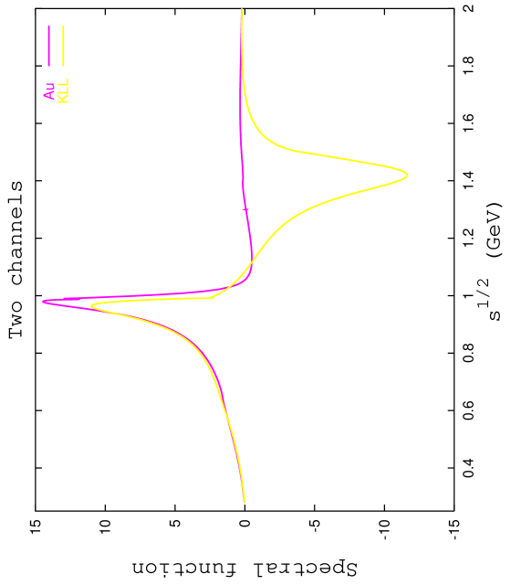
We first calculate the scalar form-factors and the spectral function from $\pi\pi-K\bar{K}$ 2-channel models. The result for the spectral function, using the T-matrix model of Au et al. [21] is shown in Fig.1, together with the result from the 2-channel version of the potential model of ref.[39]. Consider first the region $\sqrt{s}\leq 1$ GeV: there, the spectral functions from the two models have the same sign and are rather similar in shape. For sum rule applications it is useful to introduce the following spectral function integrals in this energy region

$$I_{n}=16\pi\int_{4M^{2}_{\pi}}^{4M^{2}_{K}}{Im\Pi_{6}(s)\over s^{n}}\,ds\ .$$ (42)

Some numerical results for the integrals $I_{n}$, $n=0,1$ are shown in table 1 below. The predictions from the two models are seen to differ by less than 10% for these quantities.

	Au	KLL	set A	set E	set F
$I_{0}$	3.30	3.09	4.18	3.38	2.69
$I_{1}$	4.92	4.73	6.56	5.74	4.04

Table 1: Values of the integrals $I_{0}$ and $I_{1}$ (see eq.(42)) from the 2-channel T-matrices labeled as Au[21] and KLL[39]. The last three columns correspond to different parameter sets of the 3-channel T-matrix model of Kaminski et al.[40]

.

We have also computed, for these two models, the low-energy observables associated with pion form-factors. In the neighbourhood of $s=0$, one defines (we follow the notations of ref.[12])

$$F_{1}(s)=F_{1}(0)\left[1+{1\over 6}<r^{2}>^{\pi}_{s}\,s+c_{\pi}s^{2}+\ldots\right],$$ (43)

and, similarly, for the matrix element of the $\bar{s}s$ current

$$\sqrt{2\over 3}\bar{M}^{2}_{K}G_{1}(s)=d_{F}s\left[1+b_{\Delta}s+\ldots\right].$$ (44)

As shown in ref.[12] the parameter $d_{F}$ is proportional to the derivative of $F_{\pi}$ with respect to the strange quark mass. Upon using the T-matrix from Au et al., we have verified that our calculation reproduces the results obtained previously[12][43]. The numbers are displayed in table 2. We also show the results corresponding to the T-matrix from ref.[39]. The numbers quoted in the table correspond to an improved T-matrix where the $\pi\pi$ phase-shift is constrained in the low-energy region $\sqrt{s}\leq 0.6$ GeV in order to match the predictions from CHPT at two-loops for the scattering length and the scattering range[44][45] i.e. $a_{0}^{0}=0.21$, $b_{0}^{0}=0.26M^{-2}_{\pi^{+}}$. If we do not make this modification, the results from the T-matrix of ref.[39] would be only slightly different. For instance, one would have, $<r^{2}>^{\pi}_{s}=0.580\ fm^{2}$, $d_{F}=0.075\ \rm{GeV^{-2}}$, reflecting the reasonable low-energy behaviour of the T-matrix in this particular model. These results are compatible with the known low-energy coupling constants from CHPT. At order one loop, the chiral expansion of $<r^{2}>^{\pi}_{s}$ and $d_{F}$ involve the constants $L_{4}$ and $L_{5}$

$$<r^{2}>^{\pi}_{s}={24\over F_{\pi}^{2}}\left\{2L_{4}(\mu)+L_{5}(\mu)-{1\over 32\pi^{2}}\left[\log{{M^{2}_{\pi}}\over\mu^{2}}+{1\over 4}\log{{M^{2}_{K}}\over\mu^{2}}+{4\over 3}\right]\right\}$$

$$d_{F}={8{\bar{M}_{K}}^{2}\over F_{\pi}^{2}}\left\{L_{4}(\mu)-{1\over 256\pi^{2}}\left[1+\log{{\bar{M}_{K}}^{2}\over\mu^{2}}\right]\right\}\ .$$ (45)

While $L_{4}$ is not easily determined elsewhere, $L_{5}$ can be extracted from the ratio of $F_{K}/F_{\pi}$ and this gives[9] $L_{5}(M_{\rho})=1.4\pm 0.5\,10^{-3}$. Using eqs.(Figure 1) and the results from Table 2, one deduces

$$L_{4}(M_{\rho})\simeq 0.4\,10^{-3},\quad L_{5}(M_{\rho})\simeq 1\,10^{-3}\ .$$ (47)

The value of $L_{4}$ can be considered as a prediction, and the result for $L_{5}$ appears to be compatible with $F_{K}/F_{\pi}$. One must note, though, that this agreement might be somewhat fortuitous because the error of this determination is rather large. If we assume, for instance, 10% relative errors on $<r^{2}>^{\pi}_{s}$ and on $d_{F}$, the resulting uncertainty on $L_{5}$ would be $\Delta L_{5}(M_{\rho})=\pm 0.7\,10^{-3}$.

	$<r^{2}>^{\pi}_{s}$	cπ	dF	bΔ	$10^{3}\,L_{4}$	$10^{3}\,L_{5}$
Au	0.585	10.50	0.087	3.29	0.41	0.81
KLL	0.605	10.81	0.076	3.45	0.36	1.09
set A	0.609	10.86	0.134	3.12	0.61	0.62
set E	0.583	10.58	0.144	3.15	0.66	0.29
set F	0.653	11.51	0.047	3.80	0.23	1.79

Table 2: Results for some low-energy observables and corresponding chiral coupling constants at $O(p^{4})$. $<r^{2}>_{s}^{\pi}$ is in $fm^{-2}$ and other quantities in appropriate powers of GeV. The first two lines correspond to 2-channel T-matrices and the the last three lines to 3-channel models. The labeling is the same as in Table 1.

In the region $E>1$ GeV now, the spectral functions from the two models differ considerably, see Fig.1. That corresponding to the model of ref.[39] exhibits a strong resonance effect. Its contribution to the integral goes in the sense of canceling the positive contribution from the $f_{0}(980)$. This is qualitatively as expected from the WSR (19) and indicates that it seems possible to satisfy this constraint in a 2-channel model. Quantitatively, however, if one uses the set of parameters of ref.[39] without alteration, one finds that the contribution from the $f_{0}(1500)$ is somewhat too strong and overcompensates that of the $f_{0}(980)$. At any rate, in the 1.5 GeV region it is no longer a good approximation to retain only two channels in unitarity relations. Other two-body channels are open like $\eta\eta$, and experiment indicates significant coupling of the $f_{0}(1500)$ to the $4\pi$ channel as well. We will now investigate how such additional channels can affect the results in an approximation of a single effective additional channel.

B. Three-channel models

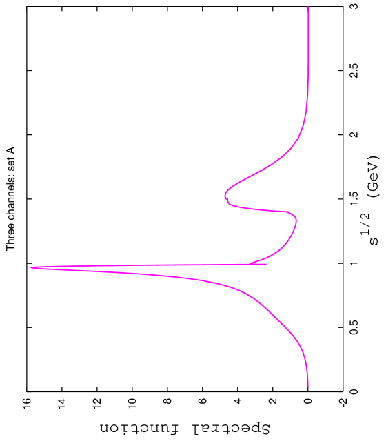
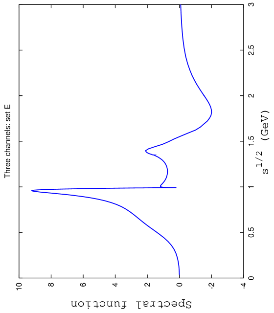
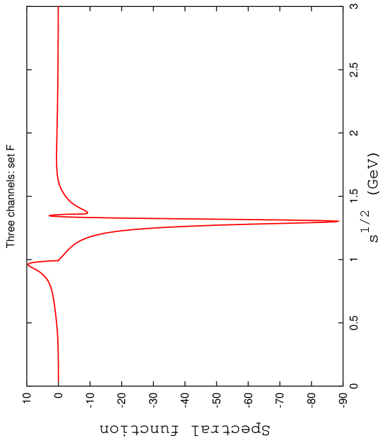
We have computed the spectral function based on the 3-channel T-matrix model from ref.[39] using several parameter sets determined in this reference and in a subsequent one[40]. Results are shown in Figs.2-4. Fig.2 corresponds to the parameter set A from ref.[39] (we recall that set B from this reference was discarded because $T_{12}$ has an unphysical low-energy pole in this case) and figs.3,4 correspond to the sets E and F from ref.[40] respectively. Again, let us consider first the energy region $\sqrt{s}\leq 1$ GeV: there, the spectral functions from the 3-channel models are comparable to those from the 2-channel ones. This can be seen, for instance, for the integrals $I_{0}$ and $I_{1}$ displayed in table 1. Also one can see from Table 2 that the result for $<r^{2}>^{\pi}_{s}$ are rather stable. A somewhat less stable quantity is $d_{F}$, the derivative of the pion form-factor of the $\bar{s}s$ current, which increases in the 3-channel model for parameter sets A and E. This results in a slight increase of $L_{4}$ and a significant decrease of $L_{5}$ which becomes too small and incompatible with $F_{K}/F_{\pi}$. On the contrary, a large value of $L_{5}$ emerges if one uses parameter set F. Keeping in mind the uncertainty in the determination of $L_{5}$ from the scalar form-factors, none of the 3-channel parameter sets considered here is as satisfactory as the 2-channel models as far as the very low energy behaviour of the form-factors is concerned.

Let us now consider the energy region $E>1$ GeV. One observes from Figs.2-4 that a variety of shapes can get generated from different parameter sets. Set F (see Fig.4 ) has a negatively contributing resonance, but it is much too strong and does not obey the WSR eq.(19). Set A has a positively contributing resonance and does not obey the WSR constraint either. Set E (see Fig.3) displays a more complicated structure: the $f_{0}(1500)$ has also a positive contribution but there is a wide negative contribution centered at 1.7 GeV, and the WSR is approximately obeyed.

C. Estimate of $\bar{\Pi}_{6}(0)$

The main conclusion from the above results is that while there seems to be reasonable agreement on the shape of the spectral function in the energy range $\sqrt{s}\leq 1$ GeV, its structure above 1 GeV is subject to considerable uncertainty. In models with more than two coupled channels the parameters are not sufficiently constrained from the experimental $\pi\pi$ and $K\bar{K}$ data. Another source of uncertainty in those models which, again, can be checked to affect the spectral function above one GeV concerns the values of the form-factors at the origin $F_{i}(0),\ G_{i}(0),\ i\geq 3$ which are not given from chiral symmetry. At least, we have seen that there exist models which fit the data and can also accomodate the WSR constraint.

In order to calculate $\bar{\Pi}_{6}(0)$ from the spectral representation eq.(21) one needs, in principle, to know the spectral function both below and above 1 GeV. However, the lower energy range is expected to generate the largest contribution. Qualitative information on the high energy sector, such as the existence of the WSR constraint and the experimental position of the resonances is sufficient if one is not asking for a very high precision. Firstly, we expect the contribution to $\bar{\Pi}_{6}(0)$ from the range $\sqrt{s}>1$ GeV to be negative, giving the upper bound,

$$\bar{\Pi}_{6}(0)\mathrel{\raise 2.58334pt\hbox{$<$}\kern-7.7778pt\lower 2.79857pt\hbox{$\sim$}}{1\over 16\pi^{2}}I_{1}\ .$$ (48)

The most plausible scenario is that of a single resonance dominated contribution around $\sqrt{s}\simeq 1.5$ GeV. In this scenario, the following estimate of $\bar{\Pi}_{6}(0)$ is valid,

$$\bar{\Pi}_{6}(0)\simeq{1\over 16\pi^{2}}\left(I_{1}-{I_{0}\over(1.5)^{2}}\right)\ ,$$ (49)

in which the WSR has been used. In this case, the correction from the higher energy range is approximately 30%. The other possibility is that several resonances, the $f_{0}(1500)$ and the $f_{0}(1700)$, are playing a role in the sum rules. If the two resonances make negative contributions one expects that the correction to $\bar{\Pi}_{6}(0)$ will be smaller than 30% because the $1/s$ factor suppresses the $f_{0}(1700)$ contribution. If the contribution from the $f_{0}(1500)$ is positive the correction is even smaller (this was realised in one of the 3-channel models considered above). The last possibility is that of a negative $f_{0}(1500)$ and a positive $f_{0}(1700)$ in which case the contribution from the higher energy region will be largest, but simple estimates like (49) show that a 50% correction is a generous upper limit. This gives us a lower bound on $\bar{\Pi}_{6}(0)$,

$$\bar{\Pi}_{6}(0)\mathrel{\raise 2.58334pt\hbox{$>$}\kern-7.7778pt\lower 2.79857pt\hbox{$\sim$}}{1\over 32\pi^{2}}I_{1}\ .$$ (50)

From these considerations and the numbers of table 1 we infer that the value of $\bar{\Pi}_{6}(0)$ must lie in the following range

$$2\mathrel{\raise 2.58334pt\hbox{$<$}\kern-7.7778pt\lower 2.79857pt\hbox{$\sim$}}16\pi^{2}\bar{\Pi}_{6}(0)\mathrel{\raise 2.58334pt\hbox{$<$}\kern-7.7778pt\lower 2.79857pt\hbox{$\sim$}}6\ .$$ (51)

Using chiral perturbation theory to one loop, eq.(10), this result can be recast into an estimate of the coupling constant $L_{6}$

$$0.4\mathrel{\raise 2.58334pt\hbox{$<$}\kern-7.7778pt\lower 2.79857pt\hbox{$\sim$}}10^{3}L_{6}(M_{\eta})\mathrel{\raise 2.58334pt\hbox{$<$}\kern-7.7778pt\lower 2.79857pt\hbox{$\sim$}}0.8\ .$$ (52)

We note that the bound (18) obtained in sec.3 is satisfied. This number can be compared with the estimate of ref.[9]

$$L_{6}(M_{\eta})=(0.0\pm 0.3)\,10^{-3}\ .$$ (53)

The central value there, is obtained from the assumption that the OZI rule applies. Indeed, the OZI rule implies that $\tilde{R}_{32}$ is identically equal to one, and inserting $L_{6}(M_{\eta})=0$ in eq.(4) one finds $\tilde{R}_{32}=0.96$ which is very close to one.

The value of $L_{6}$ that we obtained from the sum rule implies the following result for the ratio of quark condensates $\tilde{R}_{32}$

$$\tilde{R}_{32}\simeq 1-0.54\pm 0.27\ .$$ (54)

In order to obtain this estimate, we have used for $L_{6}$ the central value which emerges from the sum rule discussion above and, for the error, we have used the same value as that estimated in ref.[9] (see eq.(53) ). Within the substantial error band, the main observation is that the deviation of the quark condensate ratio from one is negative, and it seems to be rather large.

7. Summary

We started by noting that the sensitivity of the quark condensate on $N_{f}$ can be tested by studying its variation as a function of the strange quark mass. This variation may be related to the correlation function $\Pi_{6}(q^{2})$. Two different expressions of $\Pi_{6}(0)$ are equalled, one based on chiral perturbation theory and one which uses a dispersive representation. We discussed the spectral function which enters this dispersive integral. We first argued that $Im\Pi_{6}$ satisfies a Weinberg-type sum rule. This sum rule essentially relates resonance contributions from the two energy regions, $0\leq s\leq 1$ ${\rm GeV}^{2}$ and $1\leq s\mathrel{\raise 2.58334pt\hbox{$<$}\kern-7.7778pt\lower 2.79857pt\hbox{$\sim$}}4$ ${\rm GeV}^{2}$. In the first energy region the spectral function can be expressed with good accuracy in terms of scalar form-factors of the pion and the kaon. In turn, these form-factors can be constructed from experimental scattering data on $\pi\pi$ and $K\bar{K}$ following the method of ref.[12]. The determination of the spectral function in the higher energy range is more uncertain. We considered the prediction from a model which treats the $4\pi$ channel as an effective two-body channel. The influence of including this third channel in unitarity relations was found to have relatively minor influence on results in the lower energy region but has a strong influence on the region above one GeV. The dispersive integral, fortunately, receives its main contribution from the lower energy range. Using experimental information on the position of the resonances, as well as the WSR constraint, allowed us to obtain an estimate of $\bar{\Pi}_{6}(0)$.

The conclusion of this analysis is that the properties of the $f_{0}(980)$ meson translate into a value of the coupling constant $L_{6}$ which is significantly different from that expected from the OZI rule (or, alternatively, from large $N_{c}$ considerations). If one uses the central value obtained for $L_{6}$, one finds that the condensate ${\bar{u}u}$ decreases by as much as a factor of two as one decreases the mass of the strange quark mass from its physical value down to zero. A qualitatively similar behaviour is expected if one varies $N_{f}$ from $N_{f}=2$ to $N_{f}=3$. This surprising result is possibly suggesting that $N_{f}=3$ is not extremely far from a chiral phase transition point. One must bear in mind, however, that the relationship that we used between $\Pi_{6}(0)$ and the condensate ratio receives corrections from two-loop CHPT. It remains to be seen whether these are significant or not.

Acknowledgments Robert Kaminski is thanked for discussions and communicating several data files. Jan Stern is thanked for discussions, suggestions and comments on the manuscript. This work is partly supported by the EEC-TMR contract ERBFMRXCT98-0169.

Appendix: Numerical method

The general idea for solving a linear integral equation is to approximate it by an ordinary linear system of equations by discretising the integral. The main difficulty in the case of the MO equation is to handle the principal-value integral with high accuracy. Let us illustrate the method we have used on the one-channel MO equation, the generalisation to several channels is straightforward. First, one can transform the equation into one for the real part of the form-factor, $R(s)=Re(F(s))$,

$$R(s)={1\over\pi}\mathrel{\hbox{$\displaystyle\int$}\kern-5.24994pt\hbox{$-$}}_{4M^{2}}^{\infty}ds^{\prime}\,{1\over s^{\prime}-s}X(s^{\prime})R(s^{\prime})\quad X(s^{\prime})=\tan\delta(s^{\prime}).$$ (55)

It is useful to split the integration region into several sub-intervals in order to accommodate fast variations of the integrand (we have used up to seven intervals in our numerical work). Then, every sub-interval $[a,b]$ is mapped to $[-1,1]$ and the the quantity $X(s^{\prime})R(s^{\prime})$ is expanded over a basis of Legendre polynomials. This allows us to perform the principal value integration in (55) using the exact formula[46],

$$\int_{-1}^{1}du\,{P_{L}(u)\over u-z}=2Q_{L}(z)$$ (56)

Here $Q_{L}(z)$ is the so-called Legendre function of the second kind. It is crucial, in order to ensure the success of the calculation, that it be computed to very high accuracy. An algorithm, based on using the recursion relations in the forward direction if $|z|<1$ and in the backward direction otherwise, proves adequate. One obtains a discretised approximation to the integral over $[a,b]$

$$\mathrel{\hbox{$\displaystyle\int$}\kern-5.24994pt\hbox{$-$}}_{a}^{b}ds^{\prime}{1\over s^{\prime}-s_{k}}X(s^{\prime})R(s^{\prime})\approx\sum_{i=1}^{N}\hat{W}_{i}\left[1+{2(s_{k}-b)\over b-a}\right]X(s_{i})R(s_{i})$$ (57)

where

$$s_{i}={1\over 2}(a+b+(b-a)u_{i}),\quad\hat{W}_{i}[z]=-w_{i}\,\sum_{j=0}^{N-1}(2j+1)P_{j}(u_{i})Q_{j}\left(z\right)\ ,$$ (58)

and $u_{1},\ldots,u_{N}$ are the set of N Gauss-Legendre integration points (i.e. the zeros) of $P_{N}(u)$ and $w_{1},\ldots,w_{N}$ are the associated set of weights. In the case where $b=\infty$ (last sub-interval), we use

$$s_{i}={2a\over 1-u_{i}}$$ (59)

and

$$\mathrel{\hbox{$\displaystyle\int$}\kern-5.24994pt\hbox{$-$}}_{a}^{\infty}ds^{\prime}{1\over s^{\prime}-s_{k}}X(s^{\prime})R(s^{\prime})\approx{2a\over s_{k}}\sum_{i=1}^{N}\hat{W}_{i}\left[1-{2A\over s_{k}}\right]{X(s_{i})R(s_{i})\over 1-u_{i}}$$ (60)

In this manner, the functional equation for the function $R(s)$ gets transformed into a set of $M$ linear equations for $R(s_{1}),\ldots,R(s_{M})$ where $M=nN$, $n$ being the number of sub-intervals. We note that this is a homogeneous system which, strictly speaking, has no nontrivial solution unless the determinant vanishes. In practice, it does not exactly vanish. It is only in the limit of $N\to\infty$, in fact, that the determinant vanishes. In addition, one wants to specify the value at zero $R(0)$ and this generates one additional equation, which is non-homogeneous. A solution can be defined by dropping one of the homogeneous equations. A numerically stable way of performing this, is to use the singular-value decomposition of the $(M+1)\times M$ matrix of the linear equation system[47].

We have performed several checks of the numerical calculations: a) we have verified that upon using the T-matrix of the Truong-Willey type [38] the analytical result was accurately reproduced b)we have verified the stability of the result when varying the number of integration points up to several hundred points and c) we have also verified that the determinant of the n-independent solutions obtained numerically accurately reproduces the result which is known analytically (see sec. 4.C).

Figure 1: Spectral function computed from T-matrix models with two coupled channels. The solid line corresponds to the T-matrix of ref.[21], the dashed line corresponds to ref.[39]

Figure 2: Spectral function computed from the 3-channel T-matrix model of ref.[39]. The curve corresponds to the parameter set A of this reference

Figure 3: Spectral function computed from the 3-channel T-matrix model of ref.[40]. The curve corresponds to the parameter set E of this reference

Figure 4: Same as Fig.3. The curve corresponds to the parameter set F.

References

- [1] N. Seiberg, Nucl. Phys. B435 (1995) 129.
- [2] T. Banks and A. Zaks, Nucl. Phys. B196 (1982) 189.
- [3] M. Knecht and J. Stern, in “The second DAPHNE physics handbook”, L. Maiani, G. Pancheri and N. Paver eds., p.169, hep-ph/9411253.
- [4] J. Stern, Two alternatives of spontaneous chiral symmetry breaking in QCD, hep-ph/9801282
- [5] R.D. Mawhinney, Nucl. Phys. Proc. Supp. 60A (1998) 306, Y. Iwasaki et al., Prog. Theor. Phys. Suppl. 131 (1998) 415, hep-lat/9804005.
- [6] T. Shäfer and E.V. Shuryak, Phys. Rev. D53 (1996) 6522.
- [7] T. Appelquist, J. Terning and L.C.R. Wijewardhana, Phys. Rev. Lett. 77 (1996) 1214.
- [8] M. Knecht and E. de Rafael, Phys. Lett. B424 (1998) 335.
- [9] J. Gasser and H. Leutwyler, Nucl. Phys. B250 (1985) 465.
- [10] J.F. Donoghue and E. Golowich, Phys. Rev. D49 (1994) 1513.
- [11] M. Davier, L. Girlanda, A. Hoecker and J. Stern, Phys. Rev. D58 (1998) 096014.
- [12] J.F. Donoghue, J. Gasser and H. Leutwyler, Nucl. Phys. B343 (1990) 341.
- [13] J. Gasser and H. Leutwyler, Ann. Phys. (NY) 158 (1984) 142.
- [14] G. Ecker, J. Gasser, H. Leutwyler, A. Pich and E. de Rafael, Phys. Lett. B223 (1989) 425.
- [15] D.B. Kaplan and A.V. Manohar, Phys. Rev. Lett. 56 (1986) 2004.
- [16] J. Stern, private communication.
- [17] S. Weinberg, “The quantum theory of fields”, Cambridge University Press (1996), vol.2, Chap.20.
- [18] C. Caso et al., Eur. Phys. Jour. C3 (1998) 1.
- [19] H. Leutwyler, Masses of the light quarks, workshop “ Yukawa couplings and the origin of mass” p.166, Gainsville (1994) hep-ph/9405330.
- [20] J. Bijnens, J. Prades and E. de Rafael, Phys. Lett. B348 (1995) 226.
- [21] K.L. Au, D. Morgan and M.R. Pennington, Phys. Rev. D35 (1987) 1633.
- [22] A. Lanaro et al. (OBELIX coll.), Nucl. Phys. A558 (1993) 13C.
- [23] C. Amsler et al. (Crystal Barrel Coll.)Phys. Lett. B322 (1994) 431.
- [24] A. Abele at al. (Crystal Barrel Coll.), Phys. Lett. B380 (1996) 453.
- [25] D. Alde et al., Nucl. Phys. B269 (1986) 485.
- [26] S.J. Lindenbaum and R.S. Longacre, Phys. Lett. B274 (1992) 492.
- [27] S.J. Brodsky and G.P. Lepage, Phys. Rev. D22 (1980) 2150.
- [28] N.I. Muskhelishvili, ”Singular integral equations”, P. Noordhof (1953), chap. 18 and 19.
- [29] R. Omnès, Nuov. Cim. 8 (1958) 316.
- [30] B.R. Martin, D. Morgan and G. Shaw, “Pion-pion interactions in particle physics”, Academic Press (1976).
- [31] B. Hyams et al., Nucl. Phys. B64 (1973) 134.
- [32] D.V. Bugg, A.V. Sarantsev and B.S. Zou, Nucl. Phys. B471 (1996) 59.
- [33] R. Kaminski, L. Lesniak and K. Rybicki, Zeit. Phys. C74 (1997) 79.
- [34] H. Becker at al., Nucl. Phys. B151 (1979) 46.
- [35] S.M. Roy, Phys. Lett. B36 (1971) 353.
- [36] V. Bernard, N. Kaiser and U.G. Meißner, Nucl. Phys. B357 (1991) 129.
- [37] A. Roessl, Pion Kaon scattering near the threshold in chiral SU(2) perturbation theory, hep-ph/9904320.
- [38] T.N. Truong and R.S. Willey, Phys. Rev. D40 (1989) 3635.
- [39] R. Kamiński, L. Leśniak and B. Loiseau, Phys. Lett. B413 (1997) 130.
- [40] R. Kamiński, L. Leśniak and B. Loiseau, Eur. Phys. Jour. C9 (1999) 141.
- [41] D. Cohen et al., Phys. Rev. D22 (1980) 2595.
- [42] A. Etkin et al., Phys. Rev. D26 (1982) 1786.
- [43] J. Gasser and U.G. Meißner, Nucl. Phys. B357 (1991) 90.
- [44] M. Knecht, B. Moussallam, J. Stern and N.H. Fuchs, Nucl. Phys. B457 (1995) 513.
- [45] J. Bijnens, G. Colangelo, G. Ecker, J. Gasser and M. Sainio, Phys. Lett. B374 (1996) 210.
- [46] M. Abramowitz and I.A. Stegun, “Handbook of mathematical functions”, Dover (1972).
- [47] W.H. Press, S.A. Teukolsky, W.T. Vetterling, B.P. Flannery, “Numerical recipes”, Cambridge Univ. Press (1996).