Neutrino Oscillations in a ”Predictive” SUSY GUT111This talk is based on work done in collaboration with T. Blazek and K. Tobe.222Ohio State University preprint OHSTPY-HEP-T-99-014
Abstract
New data on neutrino masses is very exciting. It is the first evidence for physics beyond the standard model. In this talk we discuss this data and how it may (or may not) be used to constrain theories of charged fermion masses. The talk is divided into two parts. In part I, we briefly discuss the theoretical framework for fermion masses and mixing angles as well as some of the most salient data for neutrino oscillations. In part II, we define the framework of a ”predictive” theory of fermion masses. We then consider a particular theory which makes significant testable predictions.
1 Introduction to Neutrino Oscillations
1.1 Theory
Consider the fermion mass sector of the minimal supersymmetric standard model[MSSM]. Fermion masses are defined in the superpotential []. Three 3 x 3 complex Yukawa matrices are needed to describe up, down and charged lepton masses, while is needed for neutrino masses. In the effective low energy theory, the first three matrices contain 13 observable parameters - 9 masses and 4 quark mixing angles. The superspace potential is given by
where all fields are described by two-component left-handed Weyl spinors. The two Higgs doublets couple to the quark and lepton doublets
| (4) | |||||
| . | (7) |
and the left-handed anti-quark and anti-lepton singlets. Finally, we have added three sterile neutrinos into the MSSM in order to describe neutrino masses and mixing angles. They are sterile since they have no electroweak quantum numbers. As a result, a 3 x 3 Majorana mass term with mass matrix may be added to the theory without breaking any local gauge symmetry. When the eigenvalues of are taken much larger than the weak scale we obtain the well-known see-saw mechanism.[1] We return to neutrino masses shortly, but first consider the charged fermion masses.
In a fundamental theory, presumably defined at some large scale, the quark and lepton Yukawa matrices are complex 3 x 3 matrices which encode fermion masses and mixing angles. In this basis, labeled by the subscript , the Yukawa matrices are not diagonal; while electroweak interactions are diagonal. This is the so-called weak eigenstate basis. At the weak scale the electrically neutral Higgs components obtain vacuum expectation values[vev] , , respectively, where GeV and is the Fermi constant. We then identify the charged fermion mass matrices and similarly for down and charged lepton masses. The mass matrices can each be diagonalized by two specific unitary matrices. For example, for up quarks we have
| (11) |
In this mass eigenstate basis, electroweak interactions of quarks are no longer flavor diagonal. Moreover, the CKM matrix is given by the mismatch between diagonalizing left-handed up and down quarks. We have
| (12) |
Now consider leptons. The charged lepton mass is given by
| (13) |
and is diagonalized by the transformation and similarly for left-handed anti-leptons such that
| (14) | |||||
| (18) |
For neutrinos we now have
| (19) |
The mass scale may be much larger than the weak scale; thus in the limit we can integrate the sterile neutrinos out of the superspace potential and obtain the effective dimension five operator, see figure 1 -

| (20) |
This is the Gell-Mann, Ramond, Slansky and Yanagida[1] seesaw mechanism for obtaining light Majorana neutrinos.
The dimension-5 operator is defined at the scale and must be renormalized down to where obtains a vev. The Dirac neutrino mass is defined by and finally the effective Majorana neutrino mass is given by
| (21) |
It is defined in the basis in which charged lepton masses are diagonal. This is the so-called flavor basis for neutrinos. It is in this basis that a boson takes an electron into an electron neutrino, etc. however is not necessarily diagonal. It can be diagonalized by a unitary transformation such that
| (25) |
The unitary matrix and mass eigenvalues are the observables in neutrino oscillation experiments. The indices label the neutrino flavors, while label the mass eigenstates.
So consider a process in which lepton turns (via weak W exchange) into neutrino flavor , a linear superposition of neutrino mass eigenstates, at position . A distance away the neutrino is now detected as a linear superposition of neutrinos of flavor , see figure 2.
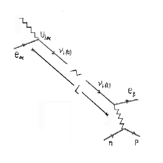
This is the process of vacuum oscillation and the probability for the state to remain is given by the formula
where
| (27) | |||||
Note, when neutrinos travel through matter there are possible matter enhanced neutrino oscillations which were discovered by Mikheyev-Smirnov and Wolfenstein [MSW].[2] These effects would take more time to describe and are beyond the scope of this talk. In what follows, we shall specifically state when MSW oscillations are the dominant effect.
1.2 Neutrino Oscillation Data
We briefly discuss the evidence for atmospheric[3], solar[4] and liquid scintillation neutrino detector [LSND][5] neutrino oscillations.
Atmospheric neutrino oscillation data
Cosmic rays incident on the upper atmosphere scatter on heavy nuclei and produce neutrinos. The neutrinos are predominantly by-products of pion and kaon decays which result in two muon type neutrinos for each electron neutrino. These neutrinos are detected at Super-Kamiokande [SuperK][3], a large water cerenkov detector located in a deep undergound laboratory in Japan. Electron and muon neutrinos scatter in the water producing electrons and muons which are distinguished by their cerenkov rings. Muons produce a sharp well-defined ring, while electrons multiple scatter in the water producing a ring with fuzzy boundaries. These atmospheric neutrinos are produced uniformly around the globe and the distance they travel to the detector is a function of the zenith angle . Neutrinos coming from above () typically travel a distance km, while neutrinos from below the detector () must travel through the earth corresponding to km. Thus atmospheric neutrinos are a natural source for testing neutrino oscillations.
Experimentalists typically analyze their data in terms of a two neutrino mixing model with mixing matrix
| (30) |
For muon neutrino oscillations where can be either or (a sterile neutrino). The persistence probability for is given by
| (31) |
where the muon neutrino energy is inferred by measuring the energy of the muon it produces.
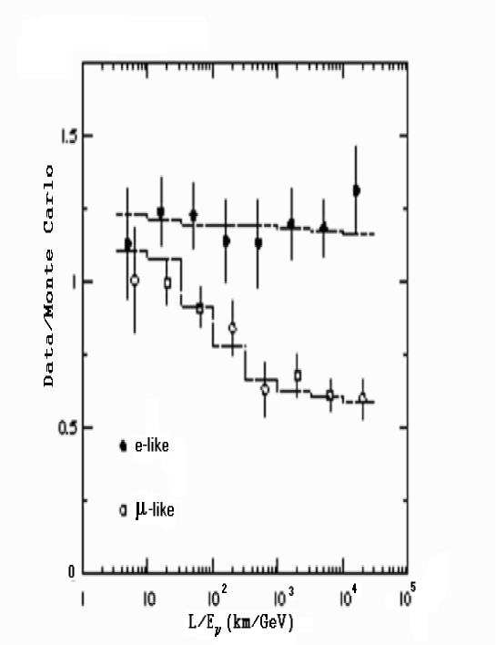
The SuperK data [3] show (see figure 3)
-
•
# depends on the zenith angle or equivalently on ,
-
•
# is independent of .
This simple observation suggests that muon neutrinos oscillate while electron neutrinos do not; hence .
After 535 days of running the best fit[3], see figure 4[3], assuming () oscillations (including the fully contained, partially contained and upward going muon data) is given by333More recent SuperK data[7] after 736 days of fully contained events and 685 days of partially contained events now gives a best fit value of
| (32) | |||||
and . We’ll come back to the question of whether or not it makes sense to consider unphysical values of .
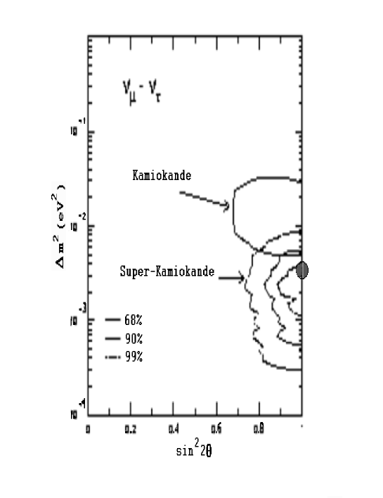
If instead () oscillations are assumed, the fit becomes worse with .
In fact, there is additional experimental data which also suggests that . This comes from the Chooz experiment[6], a neutrino detector which sits about 1 km from a nuclear reactor in France. The reactor produces electron neutrinos with a known flux. The experiment looks for the disappearance of these neutrinos. It is sensitive to the region of parameter space with and . Their null result suggests that muon neutrinos cannot oscillate into electron neutrinos with these parameters, since otherwise they would have observed a disappearance of electron neutrinos due to their oscillation into muon neutrinos.
Thus it is safe to conclude that for atmospheric neutrino oscillations. Hence we have two alternatives, or . How can this be reconciled?
We consider a recent analysis by K. Scholberg at SuperK.[7] At the moment both possibilities fit the zenith angle dependence well. It should however be possible with better statistics to distinguish vs. by the zenith angle dependence. This is because there is an MSW effect in the earth for but not for .
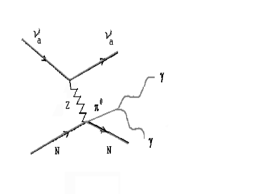
Also by considering the ratio of neutral current [NC] to charged current [CC] processes one can distinguish between the two. In this case there is preliminary data which favors . This ratio satisfies
Using SuperK data for events produced by neutral current neutrino scattering in the detector one measures (see figure 5)
Solar neutrino oscillation data
The flux of solar electron neutrinos from the sun can be calculated, see for example.[8] The result depends on the details of the solar model, but independent of which solar model is employed one finds disagreement with the data (see table 1).444Note the most uncertain component of the neutrino flux is the highest energy so-called hep neutrinos. This affects the prediction for the high energy tail of solar neutrinos.
Solar neutrino data is typically analyzed in terms of two neutrino oscillations where with , an active neutrino () or , a sterile neutrino. The results of many fits to all the data give three possible solutions with and one solution with (see table 2).[9] These solutions fall into three categories — (1) small mixing angle [SMA] MSW, (2) large mixing angle [LMA] MSW and (3) the so-called ”Just so” vacuum oscillation solution.
| MSW | SMA | |
|---|---|---|
| eV2 | ||
| LMA | ||
| eV2 | ||
| Vacuum | ”Just so” | |
| eV2 |
LSND oscillation data
The LSND experiment[5] uses a proton beam at Los Alamos National Lab to produce pions in a beam dump. Both s and s are produced. In their stopped pion data, s decay at rest into and . Note, there are no s in this decay chain. s, on the otherhand will typically be absorbed into a nucleus before they have a chance to decay.
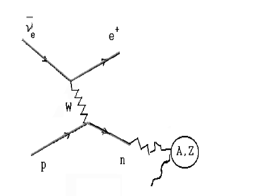
They then look for the signature of in the detector, see figure 6. The scatters on a proton and produces in the detector. The positron is observed via its cerenkov radiation. A short time later the neutron finds a nucleus and is captured, producing a gamma ray. The coincidence of these two signals is required for an event. This is the only appearance experiment and they find a signal. Once again the signal is parametrized in terms of two neutrino mixing. They find
| (35) | |||||
Summarizing neutrino oscillation data
There are some general conclusions we may draw from the above data.
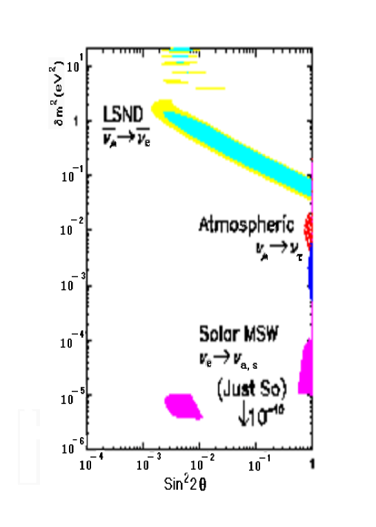
The data give three distinct scales for neutrino oscillations, see figure 7.[10]
We see
| (36) |
Thus IF all three experiments are correct, we necessarily need four light neutrinos. This of course requires sterile neutrinos.
Atmospheric neutrino oscillations, and perhaps even solar neutrinos, require maximal mixing (), while quark mixing angles are all small. We thus have
| . | (37) |
Hence any theory of fermion masses must give large mixing for leptons and small mixing for quarks. This is especially difficult in grand unified theories which relate quarks and leptons.
2 ”Predictive” SUSY GUT
At this point let me define the framework for theories of fermion masses we call a ”predictive” theory.
-
1.
It is a ”natural” theory, i.e. if one gives you the symmetries of the theory and also the states and their transformations under these symmetries, then you can write down the Lagrangian. It is the most general Lagrangian consistent with the symmetries. However, this is not sufficient.
-
2.
We also require that the number of arbitrary parameters in the theory is less than the number of observables.
A predictive theory is testable.
Clearly, to have a predictive theory one must necessarily have lots of symmetry in order to reduce the number of arbitrary parameters. The appropriate symmetry is determined by the data.
SUSY GUTs
Consider first supersymmetric grand unification or SUSY GUTs .[11] SUSY dramatically restricts the form of the Lagrangian, while GUTs unify quarks and leptons; thus quark and lepton Yukawa matrices may be related by Clebsch-Gordon coefficients. The group may be or any other simple group which breaks to the standard model gauge group at a high energy scale . Such a theory is known to be consistent with precision electroweak data. For example, given the observed values for at one finds that the running couplings unify at a scale GeV. Running the value of down from to one predicts the value of the strong coupling at the Z scale which agrees quite well with the data.
We use the GUT symmetry .[12] This is the minimal symmetry in which all fermions in one family are contained in a single irreducible representation. We have555 Note, denotes a sterile neutrino.
| (38) |
In the simplest version of one pair of Higgs doublets are contained in a . The minimal Yukawa coupling of one family of fermions to the Higgs fields is given by where is the single Yukawa coupling. If we use this minimal coupling for the heaviest generation we obtain the symmetry relation at the GUT scale. This is Yukawa unification and experimentally it is known to work quite well for the third generation[13], but fails miserably for the other two. Using the values of , one determines both and . One then predicts the value of the top quark mass[13, 14]
| (39) |
A brief digression: We note that the success of Yukawa unification has important ramifications for string theory model building. String theories, with SUSY GUTs realized as level one Kac-Moody algebras, necessarily need Wilson line breaking of the SUSY GUT down to the standard model gauge group. Unfortunately, Wilson line breaking preserves the nice feature of gauge coupling unification but typically destroys the equally nice feature of Yukawa coupling unification. This is a problem with this realization of GUTs in string theory.
Finally, whereas unifies all quarks and leptons in a single family into one irreducible representation of the group, relating up to down to charged lepton to Dirac neutrino masses, it is not sufficient to obtain a ”predictive” theory. We need more symmetry; a family symmetry to relate states of different families and to reduce the number of arbitrary parameters. Moreover family symmetry breaking can provide an understanding of the hierarchy of fermion masses and also ameliorate problems with flavor violating processes in SUSY theories.[15] To summarize, family symmetry plus GUTs are necessary for a ”predictive” theory, but they are not necessarily sufficient. It is still necessary to check in each case whether or not they sufficiently constrain the theory.
2.1 family symmetry
In this talk, we consider a particular SUSY GUT with family symmetry .[16] This model is a slight variation of the one considered previously in a paper by Barbieri et al. [BHRR].[17] The changes affect the treatment of neutrinos without affecting the predictions for charged fermion masses.
The three families transform as a doublet and a singlet under with charge (-1), (0), respectively. Note, the contained in counts +1 (-1) for every upper (lower) index. The hierarchy of fermion masses is explained by the breaking of the family symmetry. At tree level only the third family, , can couple to the of Higgs bosons which also carries no family symmetry charge. There are three ”flavon” fields in the theory transforming (under ) as (2,1,0), (3,2,1), (1,2,2) responsible for spontaneously breaking the family symmetry. The vacuum expectation values [vevs] spontaneously break to and give the second family mass. Then breaks the remaining symmetry allowing the first family to obtain mass.666It is important to have only these flavon vevs in order to retain a predictive theory.
It is important to recall that the non-abelian family symmetry can also protect against large flavor violations such as .[19]
2.2 The ”predictive” theory
This theory is completely defined by the symmetries, in this case
where denote an R symmetry for which all fields, including ” have charge +1 and a Peccei-Quinn symmetry for which all s have charge +1. The ellipsis denotes additional symmetries which exist in the fermion sector of the theory which may or may not remain unbroken in the complete theory.777One of these symmetries is needed to distinguish the fields and .
Given the states in the theory and their charges we obtain the superspace potential given by (the charge is denoted by a superscript)
| (41) |
with
The vevs of the fields ’, ” give mass to the Froggatt-Nielsen[20] states labelled by . The fields ’, ” are singlets and we use the same notation for their vevs. , on the otherhand, is a linear superposition of an singlet and adjoint with vev where are arbitrary constants which are fit to the data and are elements of the Lie algebra of with in the direction of the which commutes with and the standard weak hypercharge. Each term in has an arbitrary Yukawa coupling which is implicit. Finally, the fields are singlets; introduced to generate neutrino masses. These will be discussed in more detail shortly.
The largest scale in the theory is assumed to be the Froggatt-Nielsen masses. Below this mass scale, the states are integrated out of the theory giving the effective mass operators, see figure 8.
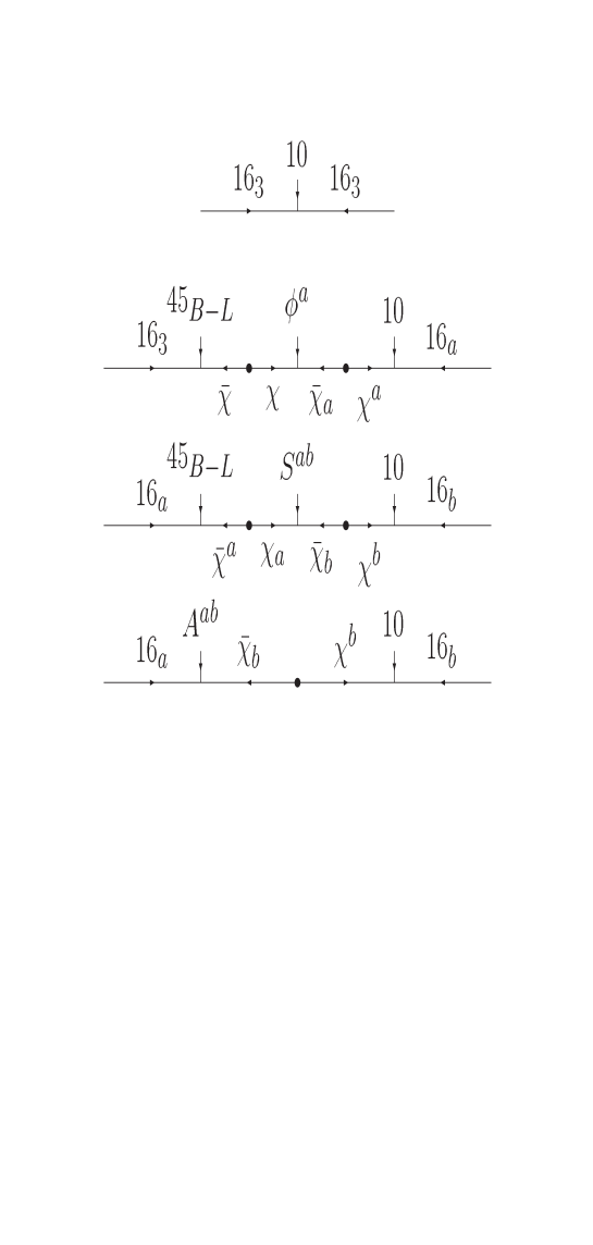
Finally, when the ”flavon” fields obtain vevs
| (44) | |||||
we generate the Yukawa couplings at a scale of order the GUT scale given by888Note the parameters are implicit functions of ratios of vevs, Yukawa couplings and .
| (48) | |||||
| (52) | |||||
| (56) | |||||
| (60) |
with
| (61) |
and
| (62) | |||||
There are six real parameters in these matrices and three phases which cannot be rotated away, which we take to be . These nine parameters are then fit to the thirteen observable charged fermion masses and quark mixing angles. Note, once these parameters are determined the Dirac neutrino mass matrix is fixed. Before we consider neutrino masses and mixing, we should first test our theory against precision electroweak data which, in our case, includes the data on charged fermion masses and mixing angles. We shall see that the fits are quite good.
2.3 Results for Charged Fermion Masses and Mixing Angles
Initial parameters: (1/) = ( GeV,%),
(r) = (),
() = ()rad,
() = () GeV,
(tan) = ()
We have performed a global analysis, incorporating two (one) loop renormalization group[RG] running of dimensionless (dimensionful) parameters from to in the MSSM, one loop radiative threshold corrections at , and 3 loop QCD (1 loop QED) RG running below . 999The predicted values of the low energy observables are highly correlated. Thus a global analysis is necessary in order to test the accuracy of the fit. We note that fermion masses and mixing angles are the precision electroweak data which constrain any theory beyond the Standard Model. It is important to know how well a theory beyond the Standard Model fits this data, even though in some cases this data still has large theoretical uncertainties. Electroweak symmetry breaking is obtained self-consistently from the effective potential at one loop, with all one loop threshold corrections included. This analysis is performed using the code of Blazek et.al.. [21] 101010We assume universal scalar mass for squarks and sleptons at . We have not considered the flavor violating effects of U(2) breaking scalar masses in this work. In this work[16], we present the results for one set of soft SUSY breaking parameters with all other parameters varied to obtain the best fit solution. In table 3 we give the 20 observables which enter the function, their experimental values and the uncertainty (in parentheses).111111 The Jarlskog parameter is a measure of CP violation. We test by a comparison to the experimental value extracted from the well-known mixing observable . The largest uncertainty in such a comparison, however, comes in the value of the QCD bag constant . We thus exchange the Jarlskog parameter for in the list of low-energy data we are fitting. Our theoretical value of is defined as that value needed to agree with for a set of fermion masses and mixing angles derived from the GUT-scale. We test this theoretical value against the “experimental” value of . This value, together with its error estimate, is obtained from recent lattice calculations.[22] In most cases is determined by the 1 standard deviation experimental uncertainty, however in some cases the theoretical uncertainty ( 0.1%) inherent in our renormalization group running and one loop threshold corrections dominates.
Given the 6 real Yukawa parameters and 3 complex phases we fit the 13 fermion mass observables (charged fermion masses and mixing angles [ replacing as a “measure of CP violation”]); we thus have 4 predictions. From table 3 it is clear that this theory fits the low energy data quite well. 121212In a future paper we intend to explore the dependence of the fits on the SUSY breaking parameters and also U(2) flavor violating effects. Note also the strange quark mass is small, consistent with recent lattice results. Finally, by adding one new parameter (a small ratio for the to Yukawa couplings) it is possible to obtain a small solution that fits charged fermion masses just as well.
Finally, the squark, slepton, Higgs and gaugino spectrum of our theory is consistent with all available data. The lightest chargino and neutralino are higgsino-like with the masses close to their respective experimental limits. As an example of the additional predictions of this theory consider the CP violating mixing angles which may soon be observed at B factories. For the selected fit we find 131313We warn the reader that according to quite standard conventions the angle is used in two inequivalent ways. tan is the ratio of Higgs vevs in the minimal supersymmetric standard model; while refers to the CP violating angle in the unitarity triangle, measured in B decays. We hope that the reader can easily distinguish the two from the context.
| (63) |
or equivalently the Wolfenstein parameters
| . | (64) |
3 Neutrino Masses and Mixing Angles
The parameters in the Dirac Yukawa matrix for neutrinos (eqn. 52) mixing are now fixed. Of course, neutrino masses are much too large and we need to invoke the GRSY [1] see-saw mechanism.
Since the 16 of SO(10) contains the “right-handed” neutrinos , one possibility is to obtain Majorana masses via higher dimension operators of the form
| (65) | |||
If field gets a vev in the ”right-handed” neutrino direction, then we obtain a mass of order . This possibility has been considered in the paper by Carone and Hall.[23]
The second possibility, which we follow, is to introduce SO(10) singlet fields and obtain effective mass terms and using only dimension four operators in the superspace potential. To do this, we add three new SO(10) singlets {} with U(1) charges { , +1/2 }. These then contribute to the superspace potential (see equation LABEL:eq:Wneutrino). Note the field with U(1) charge is assumed to get a vev in the “right-handed” neutrino direction; this vev is also needed to break the rank of SO(10).
Finally in order to allow for the possibility of light sterile neutrinos we introduce a U(2) doublet of SO(10) singlets or a U(2) singlet . They enter the superspace potential as follows –
| (66) |
We show that if the dimensionful parameters are of order the weak scale, then the sterile neutrinos (predominantly s) are light. The notation is suggestive of the similarity between these terms and the term in the Higgs sector. In both cases, we add supersymmetric mass terms and in both cases we need some mechanism to keep these dimensionful parameters small compared to the Planck scale. This may be accomplished by symmetries, see for example ref. [24].
We define the 3 3 matrix
| (70) |
The matrix determines the number of coupled sterile neutrinos, i.e. there are 4 cases labeled by the number of neutrinos ():
-
•
() 3 active ();
-
•
() 3 active + 1 sterile
();
-
•
() 3 active + 2 sterile
();
-
•
() 3 active + 3 sterile
();
In this talk we consider the cases and 4.[16]
The generalized neutrino mass matrix is then given by 141414This is similar to the double see-saw mechanism suggested by Mohapatra and Valle.[25], see figure 9 -
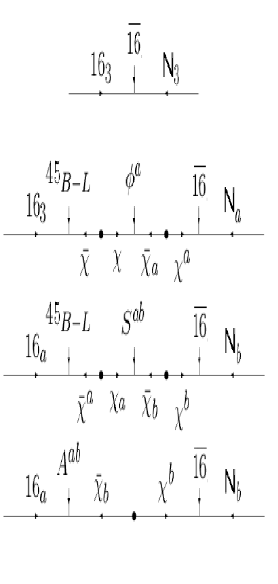
| (72) | |||
| (77) |
where
| (78) |
and
| (82) | |||||
| (86) |
are proportional to the vev of (with different implicit Yukawa couplings) and are up to couplings the vevs of , respectively.
Since both and are of order the GUT scale, the states may be integrated out of the effective low energy theory. In this case, the effective neutrino mass matrix is given (at ) by 151515In fact, at the GUT scale we define an effective dimension 5 supersymmetric neutrino mass operator where the Higgs vev is replaced by the Higgs doublet Hu coupled to the entire lepton doublet. This effective operator is then renormalized using one-loop renormalization group equations to . It is only then that is replaced by its vev. (the matrix is written in the () flavor basis where charged lepton masses are diagonal)
| (87) |
| (90) |
with
| (93) | |||||
is the unitary matrix for left-handed leptons needed to diagonalize (eqn. 52) and represent the three families of left-handed leptons in the weak- ( mass- ) eigenstate basis for charged leptons.
The neutrino mass matrix is diagonalized by a unitary matrix ;
| (94) |
where, in this case, is the flavor index and is the neutrino mass eigenstate index. Recall, is observable in neutrino oscillation experiments.
In general, neutrino masses and mixing angles have many new parameters so that one might expect to have little predictability. However, as we shall now see, the U(2)U(1) family symmetry of the theory provides a powerful constraint on the form of the neutrino mass matrix. In particular, the matrix has many zeros and few arbitrary parameters. Before discussing the four neutrino case, we show why 3 neutrinos cannot work without changing the model.
3.1 Three neutrinos
Consider first for three active neutrinos. We find (at ) in the () basis
| (98) |
with
| (99) | |||||
where in the approximation for we use
| (100) |
valid at the weak scale.
is given in terms of two independent parameters { }. Note, this theory in principle solves two problems associated with neutrino masses. It naturally has small mixing between since the mixing angle comes purely from diagonalizing the charged lepton mass matrix which, like quarks, has small mixing angles. While, for , mixing is large without fine tuning. Also note, in this theory one neutrino (predominantly ) is massless.
Unfortunately this theory cannot simultaneously fit both solar and atmospheric neutrino data.161616We have checked however that we can fit both atmospheric and LSND data. This problem can be solved at the expense of adding new family symmetry breaking vevs 171717Such an additional vev was necessary in the analysis of Carone and Hall.[23]
| (101) |
These are the most general flavor symmetry breaking vevs. We discuss these three neutrino solutions in a future paper.[26] With the massless eigenvalue in the neutrino mass matrix is now lifted. This allows us to obtain a small mass difference between the first and second mass eigenvalues which was unattainable before in the large mixing limit for . Hence a good fit to both solar and atmospheric neutrino data can now be found for small values of . In fact, only very small values of are consistent with charged fermion masses. We note that with the addition of these two complex parameters the theory is no longer predictive. In the neutrino sector any of the three solar neutrino solutions (SMA, LMA or ”Just so”) can be obtained.[26]
In the next section we discuss a four neutrino solution to both solar and atmospheric neutrino oscillations in the theory with .
3.2 Neutrino oscillations [ 3 active + 1 sterile ]
In the four neutrino case the mass matrix (at ) is given by 181818This expression defines the effective dimension 5 neutrino mass operator at which is then renormalized to in order to make contact with data.
In the analysis of neutrino masses and mixing angles we use the fits for charged fermion masses as input. Thus the parameter is fixed. We then look for the best fit to solar and atmospheric neutrino oscillations. For this we use the latest Super-Kamiokande data for atmospheric neutrino oscillations [3] and the best fits to solar neutrino data including the possibility of “just so” vacuum oscillations or both large and small angle MSW oscillations.[4] Our best fit is found in tables 4 and 5. It is obtained in the following way.
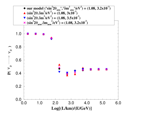
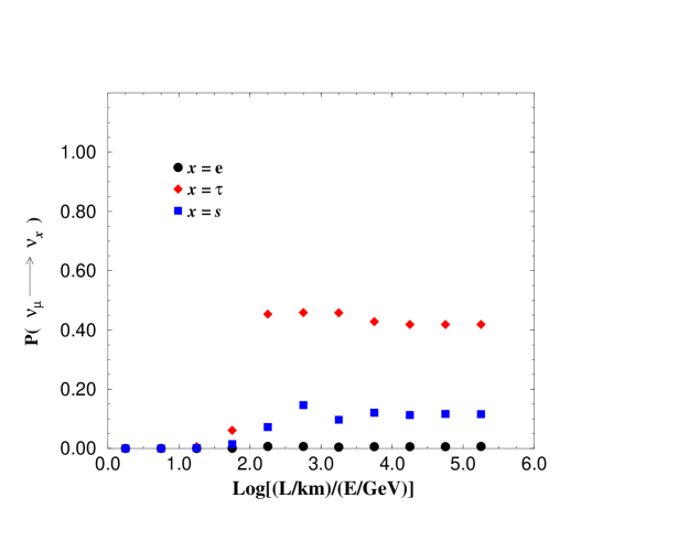
For atmospheric neutrino oscillations we have evaluated the probabilities (, ) as a function of . In order to smooth out the oscillations we have averaged the result over a bin size, x = 0.5. In fig. 10a we have compared the results of our model with a 2 neutrino oscillation model. We see that our result is in good agreement with the values of and as given.
An approximate formula for the effective atmospheric mixing angle is defined by
| (113) |
with
using the approximate relation
| (115) |
Note, may be greater than one. This is consistent with the definition above and also with Super-Kamiokande data where the best fit occurs for . In a two neutrino oscillation model, values of are unphysical and lead to negative probabilities. However in our four neutrino model, values of are perfectly physical. In figure 11, we compare the un-averaged probability for the two neutrino model and the four neutrino model discussed in this talk.
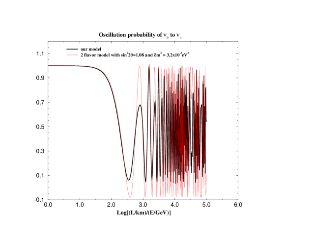
How can they give equivalent results? Experimentalists average the oscillating probability over bins in the variable . This averaging process erases the unphysical negative probabilities of the two neutrino oscillation model. It is the averaged result which compares well with the physical probability in a model with more neutrinos. Since it is much simpler to analyze the data in terms of two neutrino oscillations, it is important for experimentalists to allow for unphysical values of in their global fits. These unphysical values may just be an indication of additional neutrinos.
In fig. 10b we see however that although the atmospheric neutrino deficit is predominantly due to the maximal mixing between , there is nevertheless a significant ( 10% effect) oscillation of . This effect may be observable at Super-Kamiokande once the ratio (see 1.2, 1.2) is measured more accurately.
The oscillations or may also be visible at long baseline neutrino experiments. For example at K2K [28], the mean neutrino energy GeV and distance km corresponds to a value of x = 2.3 in fig. 2b and hence and . At Minos [29] low energy beams with hybrid emulsion detectors are also being considered. These experiments can first test the hypothesis of muon neutrino oscillations by looking for muon neutrino disappearance (for x = 2.3 we have ). Verifying oscillations into tau or sterile neutrinos is however much more difficult. For example at K2K, if only quasi-elastic muon neutrino interactions (single ring events at SuperK) are used, then this cannot be tested. Minos, on the other hand, may be able to verify the oscillations into tau or sterile neutrinos by using the ratio of neutral current to charged current measurements [29] (the so-called T test).
oscillations
Initial parameters: ( 4 neutrinos / large tan ) eV , = , = 0.278, = 3.40rad
Mass eigenvalues [eV]: 0.0, 0.002, 0.04, 0.07
Magnitude of neutrino mixing matrix Uαi
– labels mass eigenstates.
labels flavor eigenstates.
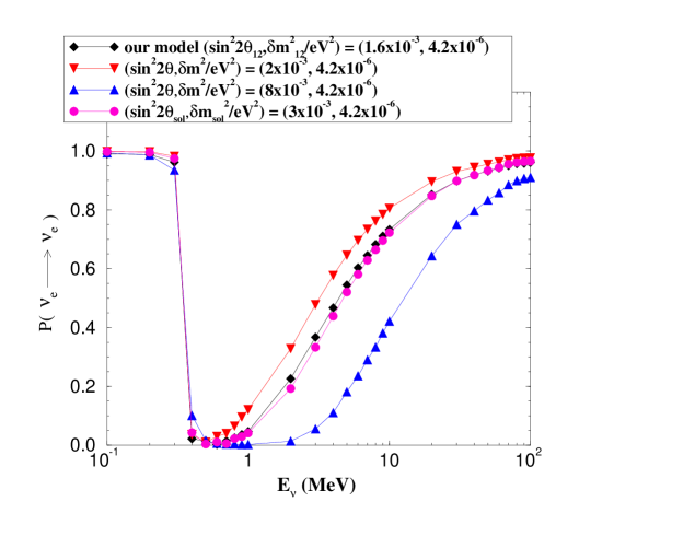
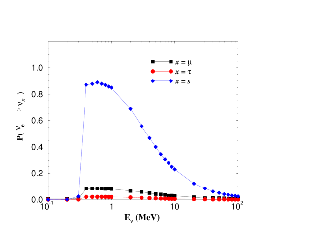
For solar neutrinos we plot, in figs. 12(a,b), the probabilities (, ) for neutrinos produced at the center of the sun to propagate to the surface (and then without change to earth), as a function of the neutrino energy Eν (MeV). 191919For this calculation we assume that electron () and neutron () number densities at a distance from the center of the sun are given by eV3 where is a solar radius. We also use an analytic approximation necessary to account for both large and small oscillation scales. For the details, see the forthcoming paper.[16] We compare our model to a 2 neutrino oscillation model with the given parameters. We see that the solar neutrino deficit is predominantly due to the small mixing angle MSW solution for oscillations. The results are summarized in tables 4 and 5.
A naive definition of the effective solar mixing angle is given by
| (116) |
In fig. 12a we see that the naive definition of underestimates the value of the effective 2 neutrino mixing angle. Thus we see that our model reproduces the neutrino results for eV2 but instead is equivalent to a 2 neutrino mixing angle instead of .
In addition, whereas the oscillation dominates we see in fig 12b that there is a sigificant ( 8% effect) for . This result may be observable at SNO [27] with threshold MeV for which .
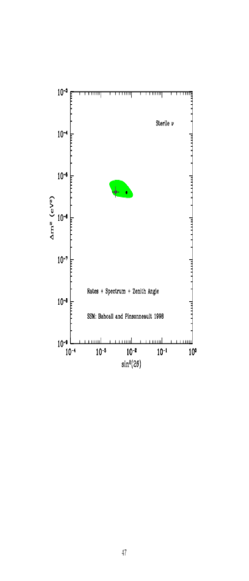
These results may be compared with a recent analysis by Bahcall, Krastev and Smirnov [BKS98][9], see figure 13. The shaded area is the 99% CL fit for sterile neutrinos consistent with the total rates, zenith-angle and recoil electron energy spectrum. The large dot is the best fit and the cross is our solution.
We note that, even though we have four neutrinos, we are not able to simultaneously fit atmospheric, solar and LSND data, i.e. it is not possible to get both and large enough to be consistent with LSND. It is worth asking however how robust is this result. Not surprisingly we find that upon introducing the new parameters (eqn. 101) a solution to all three – atmospheric, solar and LSND oscillations is obtained.[26]
Finally let’s discuss whether the parameters necessary for the fit make sense. We have three arbitrary parameters. We have taken complex, while any phases for and are unobservable. A large mixing angle for oscillations is obtained with . This does not require any fine tuning; it is consistent with which is perfectly natural (see eqn. 99). The parameter implies . Thus in order to have a light sterile neutrino we need the parameter GeV for . Considering that the standard parameter (see the parameter list in the captions to table 3) with value GeV and [eqn. 66] may have similar origins, both generated once SUSY is spontaneously broken, we feel that it is natural to have a light sterile neutrino. Lastly consider the overall scale of symmetry breaking, i.e. the see-saw scale. We have . Thus we find GeV. This is perfectly reasonable for once the implicit Yukawa couplings are taken into account.
4 Conclusions and future tests
We have discussed ”predictive” theories of charged fermion masses in this talk. These theories are constrained by lots of symmetry, in particular SUSY grand unification and family symmetries. We have argued that such ”predictive” theories may constrain neutrino masses and mixing angles as well. And vice versa, neutrino data will therefore be able to constrain theories of charged fermion masses.
We discussed a particular model with an symmetry. With minimal family symmetry breaking vevs of the form this theory is predictive. It leads to a very simple picture for neutrino oscillations. We find maximal mixing for atmospheric neutrino oscillations; a small mixing angle MSW solution with mixing for solar oscillations and NO solution for LSND.
We also made the important point that the origin of light sterile neutrinos in SUSY theories may be related to the origin of the Higgs term. In order to obtain one light sterile neutrino in our model we needed a supersymmetric mass term of the form where both are singlets and is of order .
Our model will be tested in future neutrino experiments.
-
•
For atmospheric neutrino oscillations we have . Super-Kamiokande will be able to distinguish between and by looking at the ratio of neutral current to charged current processes. A recent analysis by Super-Kamiokande[7] measures the ratio consistent with one with large errors. This result favors but the result is not yet significant. In addition, by looking at the zenith-angle dependence one may be able to distinguish between as well since for , but not , there is an MSW effect in the earth. Finally, K2K[28] and MINOS[29] will both be able to confirm the disappearance of and MINOS should eventually be able to see the appearance of .
-
•
For solar neutrino oscillations we find a small mixing angle MSW solution with . Both Super-K and Borexino[30] should be able to distinguish between small mixing angle, large mixing angle or vacuum oscillation solutions by their characteristic energy dependence and seasonal variation.[9] In addition, SNO should be able to distinguish between active and sterile neutrinos by measuring the ratio of neutral current to charged current solar neutrino processes. A ratio of order one is indicative of , while a ratio much less than one would confirm oscillations. Finally, KAMLAND[31] (similar to the CHOOZ experiment) will be sensitive to the large angle MSW oscillation region. It can thus confirm or rule out this possibility.
-
•
We find no evidence for LSND oscillations. Fortunately, this result will be tested by MiniBOONE[32]; a short base-line oscillation experiment which will be done at Fermilab.
Acknowledgments
I would like to thank my collaborators T. Blazek and K. Tobe for their help in preparing this talk. I would also like to thank the organizers of the Conference on Supersymmetry, Supergravity and Strings 99, Seoul National U., Seoul, Korea where this talk was presented and especially to Jihn E. Kim for their kind hospitality. Finally, I would like acknowledge the Institute for Theoretical Physics, Santa Barbara where this talk was written and for partial support from the National Science Foundation under Grant No. PHY94-07194. and the DOE under contract DOE/ER/01545-767.
References
- [1] M. Gell-Mann, P. Ramond and R. Slansky, in Supergravity, ed. P. van Nieuwenhuizen and D.Z. Freedman, North-Holland, Amsterdam, 1979, p. 315 ; T. Yanagida, in Proceedings of the Workshop on the unified theory and the baryon number of the universe, ed. O. Sawada and A. Sugamoto, KEK report No. 79-18, Tsukuba, Japan, 1979.
- [2] L. Wolfenstein, Phys. Rev.D17, 2369 (1978); S.P. Mikheyev and A. Yu. Smirnov, [Yad. Fiz.42, 1441 (1985) [Sov. J. Nucl. Phys.42, 913 (1985), Nuovo Cim.C9, 17 (1986).
- [3] The Super-Kamiokande Collaboration, Phys. Rev. Lett. 81 1562 (1998).
- [4] For results from the Homestake experiment, see B.T. Cleveland et al., Astrophys. J.496, 505 (1998), B.T. Cleveland et al., Nucl. Phys.B38(Proc. Supp.), 47 (1995); from SAGE, see V. Gavrin et al., in Neutrino 96, Proceedings of the XVII International Conference on Neutrino Physics and Astrophysics, Helsinki, edited by K. Huitu, K. Enquist and J. Maalampi (World Publishing, Singapore, 1997), p. 14; from GALLEX, see GALLEX Collaboration, P. Anselmann et al., Phys. Lett.B342, 440 (1995). For results from Kamiokande, see KAMIOKANDE Collaboration, Y. Fukuda et al., Phys. Rev. Lett.77, 1683 (1996); and from Super-Kamiokande, see Y. Fukuda et al., Phys. Rev. Lett. (1998), hep-ex/9805021. For recent results from Super-Kamiokande, see talk by M. Smy, DPF99, UCLA, hep-ex/9903034.
- [5] LSND Collaboration, C. Athanassopoulos et al., Phys. Rev. Lett.81 1774 (1998); ibid., Phys. Rev.C58 2489 (1998).
- [6] CHOOZ Collaboration, M. Apollonio et al., Phys.Lett. B420 397 (1998).
- [7] K. Scholberg, Talk presented at 8th International Workshop on Neutrino Telescopes, Venice, February 23-26 1999, hep-ex/9905016.
- [8] J. Bahcall, S. Basu and M.H. Pinnsoneault, Phys. Lett. B433, 1 1998.
- [9] J.N. Bahcall, P.I. Krastev and A. Yu. Smirnov, Phys. Rev.D58 096016 (1998) and references therein; V. Barger, S. Pakvasa, T. J. Weiler, K. Whisnant, Phys. Rev.D58, 093016 (1998); V. Barger, S. Pakvasa, T.J. Weiler, K. Whisnant, Phys. Lett.B437, 107-116 (1998); G.L. Fogli, E. Lisi, A. Marrone, G. Scioscia, Phys. Rev.D59, 033001 (1999); G.L. Fogli, E. Lisi, D. Montanino, Phys. Lett.B434, 333-339 (1998); S.M. Bilenky, C. Giunti, W. Grimus, hep-ph/9812360, to be published in Progress in Particle and Nuclear Physics, Volume 43. For recent analyses, see J.N. Bahcall, P.I. Krastev and A. Yu. Smirnov, hep-ph/9905220 and M.C. Gonzalez-Garcia, P.C. de Hollanda, C. Pena-Garay and J.W.F. Valle, hep-ph/9906469.
- [10] This figure is from a talk by J. Conrad, Plenary Talk presented at the International Conference on High Energy Physics (ICHEP), Vancouver, (1998), hep-ex/9811009.
- [11] S. Dimopoulos, S. Raby and F. Wilczek, Phys. Rev. D24, 1681 (1981); S. Dimopoulos and H. Georgi, Nucl. Phys.B 193, 150 (1981); L. Ibanez and G.G. Ross, Phys. Lett. 105B, 439 (1981); M. B. Einhorn and D. R. T. Jones, Nucl. Phys. B196, 475 (1982); W. J. Marciano and G. Senjanovic, Phys. Rev. D 25, 3092 (1982). For recent analyses, see P. Langacker and N. Polonsky, Phys. Rev.D47, 4028 (1993); ibid., D49, 1454 (1994); M. Carena, S. Pokorski, C.E.M. Wagner, Nucl. Phys.B406, 59 (1993).
- [12] H. Georgi, Particles and Fields, Proceedings of the APS Div. of Particles and Fields, ed C. Carlson; H. Fritzsch and P. Minkowski, Ann. Phys. 93, 193 (1975).
- [13] M. Olechowski and S. Pokorski, Phys. Lett.B214, 393 (1988); B. Ananthanarayan, G. Lazarides and Q. Shafi, Phys. Rev.D44, 1613 (1991); H. Arason et al., Phys. Rev. Lett.67, 2933 (1991); S. Kelley, J. Lopez and D. Nanopoulos, Phys. Lett.B274, 387 (1992); G. Anderson, S. Dimopoulos, L.J. Hall, S. Raby and G. Starkman, Phys. Rev.D49, 3660 (1994).
- [14] For a recent analysis, see L.J. Hall, R. Rattazzi and U. Sarid, Phys. Rev.D50, 7048-7065 (1994).
- [15] S. Dimopoulos and H. Georgi, Nucl. Phys. B193 150 (1981); L.J. Hall, V.A. Kostelecky and S. Raby, Nucl. Phys.B267 415 (1986); H. Georgi, Phys.Lett.169B 231 (1986); F. Borzumati and A. Masiero, Phys. Rev. Lett.57 961 (1986); R. Barbieri and L.J. Hall, Phys. Lett. B338 212 (1994); R. Barbieri, L.J. Hall and A. Strumia, Nucl. Phys.B445 219 (1995); J. Hisano, T. Moroi, K. Tobe, M. Yamaguchi and T. Yanagida, Phys. Lett.B357 579 (1995); F. Gabbiani, E. Gabrielli, A. Masiero and L. Silvestrini, Nucl. Phys.B477 321 (1996); S. Dimopoulos and A. Pomarol, Phys. Lett.B353 222 (1995); J. Hisano, T. Moroi, K. Tobe and M. Yamaguchi, Phys. Rev. D53 2442 (1996); ibid., Phys. Lett. B391 341 (1997); K. Tobe, Nucl. Phys. (Proc. Suppl.) B59, 223 (1997); J. Hisano, D. Nomura, T. Yanagida, Phys. Lett.B437 351 (1998); J. Hisano, D. Nomura, Y. Okada, Y. Shimizu, M. Tanaka, Phys. Rev. D58 116010 (1998); J. Hisano and D. Nomura, hep-ph/9810479.
- [16] T. Blazek, S. Raby and K. Tobe, accepted for publication in Phys. Rev.D (1999), hep-ph/9903340.
- [17] R. Barbieri, L.J. Hall, S. Raby and A. Romanino, Nucl. Phys.B493 3 (1997); R. Barbieri, L.J. Hall and A. Romanino, Phys. Lett.B401 47 (1997).
- [18] S. Dimopoulos, S. Raby and F. Wilczek, Phys. Rev.D24 1681 (1981); S. Dimopoulos and H. Georgi, Nucl. Phys.B193 150 (1981).
- [19] M. Dine, R. Leigh and A. Kagan, Phys. Rev.D48 4269 (1993); A. Pomarol and D. Tommasini, Nucl.Phys.B466 3 (1996); R. Barbieri, G. Dvali and L.J. Hall, Phys. Lett.B377 76 (1996); R. Barbieri and L.J. Hall, Nuovo Cim.110A 1 (1997).
- [20] C. Froggatt and H.B. Nielsen, Nucl. Phys.B147 277 (1979).
- [21] T. Blazek, M. Carena, S. Raby and C. Wagner, Phys. Rev.D56 6919 (1997).
-
[22]
R. Gupta, D. Daniel, G.W. Kilcup, A. Patel and S.R. Sharpe,
Phys. Rev. D47, 5113 (1993); G. Kilcup, Phys. Rev. Lett. 71, 1677 (1993); S. Sharpe, Nucl. Phys. B (Proc. Suppl.) 34, 403 (1994).
The same mean value and standard deviation for were given in a recent review article: U.Nierste,”Phenomenology of in the Top Era”, invited talk at the workshop on K physics, Orsay, France, May 30 - June 4, 1996 (LANL hep-ph/9609310). - [23] C.D. Carone and L.J. Hall, Phys.Rev.D56 4198 (1997); L.J. Hall and N. Weiner, hep-ph/9811299.
- [24] G.F. Giudice and A. Masiero, Phys. Lett.B206, 480 (1988) ; J.E. Kim and H.P. Nilles, Mod. Phys. Lett.A9, 3575 (1994).
- [25] R.N. Mohapatra and J.W.F. Valle, Phys. Rev.D34 1634 (1986).
- [26] T. Blazek, S. Raby and K. Tobe, a paper describing our results for with is in preparation.
- [27] M.E. Moorhead (SNO Collaboration), Nucl. Phys. (Proc. Suppl.) B48, 378 (1996).
- [28] M. Sakuda (K2K Collaboration), “The KEK-PS Long Baseline Neutrino Oscillation Experiment (E362)”, KEK-PREPRINT-97-254; Yuichi Oyama (K2K Collaboration) “K2K (KEK To Kamioka) Neutrino-Oscillation Experiment At KEK-PS”, KEK-PREPRINT-97-266 (hep-ex/9803014).
- [29] MINOS Collaboration, “Neutrino Oscillation Physics at Fermilab: The NuMI-MINOS Project”, NuMI-L-375. See also the MINOS web page: http://www.hep.anl.gov/ndk/hypertext/numi.html.
- [30] C. Arpesella et al., BOREXINO proposal, vols. 1 and 2, eds. G. Bellini, R. Raghavan et al. (U. of Milano, Milano, 1992).
- [31] Y. F. Wang, STANFORD-HEP-98-04 (1998); P. Alivisatos et al., STANFORD-HEP-98-03 (1998).
- [32] See http://www.neutrino.lanl.gov/BOONE E. Chruch et al., FERMILAB-P-0898-(1987).