NON-EQUILIBRIUM QUANTUM PLASMAS IN SCALAR QED: PHOTON PRODUCTION, MAGNETIC AND DEBYE MASSES AND CONDUCTIVITY.

Abstract

We study the generation of a non-equilibrium plasma in scalar QED with $N$-charged scalar fields in the cases: a) of a supercooled second order phase transition through spinodal instabilities and b) of parametric amplification when the order parameter oscillates with large amplitude around the minimum of the potential. The focus is to study the non-equilibrium electromagnetic properties of the plasma, such as photon production, electric and magnetic screening and conductivity. A novel kinetic equation is introduced to compute photon production far away from equilibrium in the large $N$ limit and lowest order in the electromagnetic coupling. During the early stages of the dynamics the photon density grows exponentially and asymptotically the frequency distribution becomes $N_{ph}(\omega)\sim\alpha\;m^{2}/[\lambda^{2}\;\omega^{3}]$ with $\lambda$ the scalar self-coupling and $m$ the scalar mass. In the case of a phase transition, electric and magnetic fields are correlated on distances $\xi(t)\sim\sqrt{t/m}$ during the early stages of the evolution and the power spectrum is peaked at low momentum. This aspect is relevant for the generation of primordial magnetic fields in the Early Universe and for photoproduction as a potential experimental signature of the chiral phase transition. Magnetic and Debye screening masses are defined out of equilibrium as generalizations of the equilibrium case. While the magnetic mass vanishes out of equilibrium in this abelian model, we introduce an effective time and wave-number dependent magnetic mass that reveals the different processes that contribute to screening and their time scales. The Debye mass turns out to be $m^{2}_{Deb}\sim\alpha\;m^{2}/\lambda$ for a supercooled phase transition while in the case of an oscillating order parameter an interpolating time dependent Debye mass grows as $\alpha\sqrt{m\,t}/\lambda$ due to a non-linear resonance at low momentum in the charged particle distribution. It is shown how the transverse electric conductivity builds up during the formation of the non-equilibrium plasma. Its long wavelength limit reaches a value $\sigma_{k\approx 0}\sim\alpha\;m/\lambda$ at the end of the stage of linear instabilities. It is shown that the electric conductivity stays finite for all $k$ including $k=0$ for finite time. In the asymptotic regime it attains a form analogous to the equilibrium case but in terms of the non-equilibrium particle distribution functions.

Contents

toc

I Introduction and motivation

The study of the dynamics of phenomena strongly out of equilibrium is very relevant in cosmology where it plays a fundamental role in the consistent description of inflationary scenarios, baryogenesis and of generation of primordial magnetic fields. Also in Relativistic Heavy Ion collisions where it now acquires further phenomenological importance since the Relativistic Heavy Ion Collider (RHIC) at Brookhaven begins operation. RHIC and the forthcoming Large Hadron Collider at CERN will probe the quark-gluon plasma and the chiral phase transitions in an extreme environment of high temperature and density. These experimental programs have inspired intense theoretical efforts to understand the formation, evolution and potential experimental signatures of the quark-gluon plasma[1, 2] as well as relaxation and transport phenomena on unprecedented short time scales. There are several fundamental questions which define to a large extent the theoretical aspects of this program: how does the quark-gluon plasma form and equilibrates from the evolution of the parton distribution functions? what are the time scales for electric and magnetic screening that dress the gluons and cut-off small angle scattering? how does a hydrodynamic picture of the space-time evolution of the plasma emerge? what are the experimental signatures?. These and other fundamental but extremely difficult questions are being addressed from many different perspectives. An important approach that seeks to describe the space-time evolution of partons is based on transport equations that describe partonic cascades starting from a microscopic description and incorporate semi-phenomenologically some screening corrections in the scattering cross sections[3, 4, 5]. A correct description of electric and magnetic screening is very important in this program since both act as infrared cutoffs in transport cross sections and determine energy losses in the plasma. Amongst the several potential experimental signatures proposed to detect the QGP, photons and dileptons are deemed to be clean probes of the quark-gluon plasma because they only interact electromagnetically[1, 2, 6] and their mean-free paths are much larger than the size of the fireball $\approx 20\mbox{fm}$. Hence, these electromagnetic probes could provide clean signatures of equilibration or out of equilibrium phenomena unhindered by the strong interactions. Non-equilibrium phenomena associated with a quenched chiral phase transition could have potentially important electromagnetic signatures in the photon spectrum if there are strong charged pion fluctuations during the phase transition. A preliminary study in this direction was pursued in[7] where it was indicated that departures from equilibrium in the photon distribution at low momentum could provide a signature of a supercooled chiral phase transition[8]. In cosmology, post-inflationary phase transitions or the fast evolution of an inflaton field after inflation could generate the hot plasma that describes the standard big bang scenario with a radiation dominated Friedman-Robertson-Walker cosmology at the end of inflation[9]. Furthermore, non-equilibrium effects during cosmological phase transitions had been conjectured to generate the primordial magnetic fields that could act as seeds to be amplified by dynamo mechanisms as an explanation for the observed galactic magnetic fields[10, 11]. Theoretical models for generation of primordial magnetic fields involve strong fluctuations of charged fields that lead to non-equilibrium electromagnetic currents[12, 13, 14], much like the strong fluctuations in the pion fields during a possible supercooled chiral phase transition and the possibility of photon production associated with these fluctuations[7].

Thus we see that physically relevant non-equilibrium physical phenomena are common to cosmology and the quark-gluon plasma and chiral phase transition and it has been conjectured that indeed primordial electromagnetic fields can be generated from strong electromagnetic fluctuations at the quark-hadron phase transition[15, 16]. An important ingredient both in the quark-gluon plasma as well as in the formation of astrophysical and cosmological plasmas is a description of the transport properties, in particular the screening masses and the electrical conductivity. Screening masses are an important ingredient in charmonium suppression which is one of the potential probes of the QGP[17] and regulate the infrared behavior of transport coefficients[18, 19].

The electrical conductivity plays an important role in the formation and correlations of primordial magnetic fields in the early universe and contributes to ohmic heating and therefore energy losses and entropy production in the QGP. The electrical conductivity in the early universe was estimated in[11] and (equilibrium) screening corrections were included in[20]. More recently the electrical conductivity of the plasma at temperatures near the electroweak scale was calculated in[21] including Debye and dynamical (Landau damping) screening of electric and magnetic interactions.

Hence, there are common relevant problems in cosmology, astrophysics and ultrarelativistic heavy ion collisions that seek a deeper understanding of the physics of the formation of a plasma beginning from a non-equilibrium initial state of large energy density, its evolution, the onset of electric and magnetic screening phenomena and the generation of seeds of bulk electric and magnetic fields, i.e. photon production.

A first principles description of the formation of a hot plasma and its dynamical evolution from an initial state of large energy density beginning from QCD or the Standard Model would be a desirable goal, but clearly an extremely complicated task.

The goals of this work:

In this article we study a model that bears many of the important aspects of QCD and the Standard Model which combined with a non-perturbative framework allows us to provide quantitative and qualitative answers to many of the questions associated with the formation and evolution of a non-equilibrium plasma.

The model that we propose to study is scalar QED with $N$-charged scalar fields coupled to one $U(1)$ photon field and one neutral scalar field that plays the role of an order parameter for a phase transition. The model is such that the $U(1)$ local gauge symmetry associated with the photon field is not spontaneously broken much in the same manner as the usual electromagnetic field in the Standard Model. Besides, this model being a suitable framework to study the questions posed above, we will argue that it is potentially relevant to the description of photon production during the chiral phase transition of QCD. Therefore, the dynamics and mechanisms revealed in this model could prove to be very valuable in the description of the generation of primordial magnetic fields during one of the QCD phase transitions in the early universe and also in photon production during the chiral phase transitions in heavy ion collisions.

Furthermore scalar QED has been shown to share many properties of spinor QED and QCD in leading order in the hard thermal loop approximation[27, 32], hence the model studied in this article can serve as a useful and relevant testing ground to study similar questions in QED and QCD.

Since the non-equilibrium processes that lead to the formation of the plasma are non-perturbative, we resort to the large $N$ limit as a consistent framework to study the non-perturbative dynamics. We take the electromagnetic coupling to be perturbative and compute various quantities, such as the rate of photon production, magnetic and Debye masses and the transverse conductivity to leading order in the large $N$ limit and to lowest order in the electromagnetic coupling, discussing the validity of weak coupling in each case.

The focus of this work centers on the following aspects: i) The description of the formation of a non-equilibrium plasma of charged particles during a stage of strong non-equilibrium evolution beginning from an initial state of large energy density. ii) The production of photons and therefore of electric and magnetic fields from the strong fluctuations of the charged fields. This aspect is relevant for the formation of primordial magnetic fields in the early universe and also for photon production during non-equilibrium stages for example of the chiral phase transition, where the charged fields would be the pions. iii) The dynamical aspects of electric and magnetic screening. We study in detail the magnetic and Debye masses and the time scale of the different processes that contribute to screening. iv) The non-equilibrium transverse electrical conductivity. We analyze in detail the build-up of conductivity as the plasma is forming and its asymptotic limit, comparing to the equilibrium case.

In particular two important situations are studied: a): a ‘quenched’ (or supercooled) second order phase transition in which the initial state of large energy density is the false vacuum (the quantum state is localized at the top of the potential). The dynamics in this case is described by the process of spinodal decomposition and phase separation, characterized by the exponential growth of long-wavelength unstable fluctuations. These instabilities and the ensuing large fluctuations of the charged fields and particle production result in the formation of a non-equilibrium plasma and the non-perturbative production of photons and therefore of electric and magnetic fields. The spinodal instabilities are shut-off by the non-linearities and the resulting plasma possesses a non-equilibrium distribution function of charged scalars peaked at low momenta. b): The stage of large amplitude oscillations of the order parameter around the minimum of the potential. This stage arises for example after a phase transition in which the order parameter has rolled down the potential hill and is oscillating around one of the minima of the potential. Such would be the case in the case of the chiral phase transition where a small explicit symmetry breaking term (that gives mass to the pions) will force the isoscalar order parameter to evolve towards the minimum. This stage is characterized by parametric amplification of quantum fluctuations of the charged fields and again results in non-perturbative production of charged scalars and of photons[7]. This stage is also relevant in cosmology and describes the reheating process after an inflationary phase transition or in chaotic inflationary models[9]. The phenomenon of parametric amplification of quantum fluctuations during the oscillatory phase of the order parameter, the inflaton in the cosmological setting, has been recognized as a very efficient mechanism of particle production and reheating in the early universe[24, 25]. Parametric amplification of pion fluctuations after a supercooled chiral phase transition has also been recognized to be an important possibility in heavy ion collisions[26]. Both non-equilibrium phenomena are non-perturbative in the scalar quartic self-coupling. Therefore, the dynamics in the scalar sector is studied consistently in leading order in the large $N$ expansion, while electromagnetic phenomena are studied to lowest order in $\alpha$.

Spinodal instabilities or parametric amplification of quantum fluctuations of charged fields result in the formation of a non-equilibrium plasma. In both cases strong fluctuations in the electromagnetic currents result in the production of photons i.e. electric and magnetic fields as well as screening currents generating screening masses and an electrical conductivity in the medium.

Thus, our main objectives are to study the dynamics of formation of the non-equilibrium plasma, photon production and the power spectrum in the generated electric and magnetic fields, the onset of electric and magnetic screening phenomena described in real time and the build up of conductivity in the medium. Equilibrium aspects of hot scalar QED had been previously studied[27, 28] and we will compare the non-equilibrium aspects to the equilibrium case to highlight the differences and similarities.

Results: a) Photon production:

We have derived a consistent kinetic equation to describe photon production in situations strongly out of equilibrium and used this equation to lowest order in $\alpha$ (the electromagnetic coupling) and leading order in the large $N$ limit for the charged fields, to obtain the spectrum of photons produced via spinodal and parametric instabilities. In the case of spinodal instabilities which correspond to the case of a supercooled (second order) phase transition we have obtained the power spectrum and correlation function of the electric and magnetic fields generated during the non-equilibrium stage. We find that there is a dynamical correlation length that grows as $\xi(t)\sim\sqrt{t}$ at short times. It determines the spatial correlations of the electromagnetic fields. The power spectrum is peaked at long-wavelength with an amplitude $\sim\alpha/\lambda^{2}$ with $\lambda$ the quartic self-coupling of the charged scalar fields. In the case of parametric amplification the power spectrum peaks near the center of parametric resonance bands; the amplitude being also $\sim\alpha/\lambda^{2}$ but the electric and magnetic fields have small correlation lengths. In the asymptotic regime the distribution of produced photons as function of frequency $\omega$ behaves as $\sim\alpha\;m^{2}/[\omega^{3}\;\lambda^{2}]$. This entails a logarithmically infrared divergent number of photons but a finite total energy. In the case when the plasma is generated by spinodal instabilities, the asymptotic photon distribution continues to grow proportional to $\log m\tau$ due to collinear singularities. These behaviors points to the necessity of a resummation perhaps via the dynamical renormalization group introduced in reference[46].

b) Magnetic and Debye screening masses: We introduce a definition of the magnetic and Debye screening masses out of equilibrium which are the natural extension of that in equilibrium[29, 31, 32]. We find that the magnetic mass out of equilibrium vanishes at order $\alpha$ through cancellations akin to those that take place in equilibrium. Furthermore, we introduce an effective magnetic mass that describes non-equilibrium screening phenomena for long-wavelength fluctuations as a function of time and which reveals the different time scales of the processes that contribute to the cancellation of the magnetic mass. Asymptotically for long times and in the long-wavelength limit we find that processes which are the non-equilibrium counterpart of Landau damping contribute on time scales which are much longer than typical production and annihilation processes.

The extrapolation of this time dependent effective magnetic mass to the zero momentum limit at finite time reveals an unexpected instability in the time evolution of transverse electromagnetic mean fields during the time scales studied in this article. This is a rather weak instability presumably related to photon production although the precise relation is not clear and deserves further study.

In the case of spinodal instabilities we find that the (electric screening) Debye mass at leading order in $e^{2}$ and $1/N$ is finite and given by $m^{2}_{Deb}=8\;|m_{R}|^{2}\;e^{2}/\lambda+{\cal O}(1)$. In the case of parametric amplification the Debye mass grows monotonically with time as $\sqrt{t}$ times a coefficient of order ${\cal O}(e^{2}/\lambda)$. This result is a consequence of non-linear resonances [37] which make the charged particle distribution strongly peaked at small momentum, ${\cal N}_{k}(t=\infty)\sim|m_{R}|^{2}/[\lambda\;k^{2}]$. Since the Debye mass is determined by the derivative of the distribution function, the singularity at small momentum results in a divergent Debye mass for asymptotically long time. This result, valid to first order in $\alpha$, strongly suggests that a resummation of electromagnetic corrections will be required in the case of parametric resonance. Such a program lies outside the scope of this work and will be the subject of a forthcoming study.

c) Transverse electric conductivity: As the plasma of charged particles forms the medium becomes conducting. We study the transverse electrical conductivity from linear response out of equilibrium (Kubo’s conductivity) as a function of time to lowest order in the electromagnetic coupling. The early time behavior during the stage of spinodal or parametric instabilities results in a rapid build up of the conductivity which attains a non-perturbative value ${\cal O}(\alpha\;m/\lambda)$ at the end of this stage. We find that the conductivity is finite for all $k$ (including $k=0$) at finite time. Asymptotically at long times, the conductivity attains a form similar to the equilibrium case (to lowest order in $\alpha$) but in terms of the non-equilibrium distribution functions.

This feature of the asymptotic conductivity must apply to other physical magnitudes for asymptotic times. Namely, one can compute their $t\to\infty$ limit just replacing the thermal occupation numbers in their equilibrium expression by the out-of-equilibrium distribution functions.

The article is organized as follows: in section II the model is introduced and the large $N$ limit is described. In section III we review the main features of spinodal decomposition and parametric amplification and introduce the relevant non-equilibrium Green’s functions necessary for the calculations. In section IV we study photon production both during the early stages of the instabilities as well as at asymptotically long times, In section V we study photon production in equilibrium to contrast and compare to the non-equilibrium results. In section VI we study magnetic screening and the magnetic mass out of equilibrium. Just as in the equilibrium case in this abelian theory, we show that the magnetic mass vanishes, but point out the different time scales for the processes involved. A suitably defined effective magnetic mass describes non-equilibrium aspects of magnetic screening on intermediate time scales. Section VII studies the Debye (electric) screening mass, and it is argued that in the case of parametric amplification the Debye mass diverges because as a result of a singular distribution function for the charged scalars at low momentum. In section VIII we study Kubo’s (linear response) transverse electrical conductivity to lowest order in $\alpha$. In particular we focus on the build-up of conductivity during the early stages of formation of the plasma. We compare the conductivity in the asymptotic time regime to the result in equilibrium. Our conclusions are summarized in section IX. Here we also discuss the limit of validity of our studies and the potential phenomenological implications of the results from this model. An Appendix is devoted to a novel kinetic equation that describes photon production away from equilibrium.

II The model: SQED with $N$ charged scalars in the large $N$ limit

We focus on the non-equilibrium dynamics of the formation of relativistic quantum plasma at high density after a phase transition, either via long-wavelength spinodal instabilities in the early stages of a rapid (quenched) second order phase transition or by parametric amplification of quantum fluctuations as the order parameter oscillates around the equilibrium minimum. Previous work[25, 36, 37] revealed that both types of phenomena are non-perturbative in the scalar self-coupling, hence we propose to use the large $N$ limit as a consistent tool to study non-equilibrium phenomena non-perturbatively. Our main goals are to provide a quantitative understanding of several important processes that are of interest both in cosmology as well as in the formation of a quark-gluon plasma: i) non-equilibrium production of photons, i.e. the non-equilibrium generation of electromagnetic fields, ii) the dynamics of screening and generation of electric and magnetic masses strongly out of equilibrium, iii) the build-up of conductivity in the non-equilibrium plasma.

We consider a version of scalar quantum electrodynamics with $N$ charged scalar fields $\Phi_{r}$ to be collectively referred to as pions coupled to a neutral field $\sigma$ is such a way that the scalar sector of the theory has an $O(2N+1)$ isospin symmetry. The coupling to the electromagnetic field reduce this symmetry to an $SU(N)_{global}\times U(1)_{local}$. When we consider the breaking of the isospin symmetry, the neutral scalar field $\sigma$ will acquire an expectation value, but not the charged fields $\Phi_{r}$. There are two main reasons for this choice a) this allows to separate the Higgs phenomenon and generation of mass for the vector field from truly non-equilibrium effects and b) we seek to describe a phenomenologically relevant model, in particular the role of non-equilibrium pion fluctuations during the chiral phase transition wherein electromagnetism is not spontaneously broken by chiral symmetry breaking.

The same methods can be used to study the Higgs phenomenon out of equilibrium and we expect to report on such study in the near future. Furthermore, as we seek to describe some relevant phenomenology for low energy QCD, this model describes the large $N$ limit of the $O(4)$ gauged linear sigma model that describes the three pions. Electromagnetism is unbroken but isospin is broken by the coupling of the charged pions to electromagnetism and this is captured by the model under consideration.

In this abelian theory it is straightforward to provide a gauge invariant description by requiring that the set of first class constraints, $\Pi_{0}=0\;;\;\vec{\nabla}\cdot\vec{E}-\rho=0$ annihilate the physical states[38, 39] with $\Pi_{0}$ being the canonical momentum conjugate to the temporal component of the vector field and $\vec{\nabla}\cdot\vec{E}-\rho=0$ is Gauss’ law and $\rho$ is the charge density. This procedure is described in detail in[38, 39] where it is shown to be equivalent to a gauge-fixed formulation in Coulomb’s gauge. The instantaneous Coulomb interaction is traded by a Lagrange multiplier $A_{0}(\vec{x},t)$ not to be confused with the original temporal component of the gauge field. The issue of gauge invariance is an important one because we will study the distribution function of charged scalar fields and by providing a gauge invariant description from the beginning we avoid potential ambiguities.

In this formulation we introduce the physical fields

$$(\sigma,\Phi_{r},\Phi_{r}^{\dagger},\vec{A}_{T}^{i},A_{0}),\quad r=1,\dots,N$$

The electromagnetic potential is a physical field which satisfies the transversality condition

$$\nabla\cdot\vec{A}_{T}=0,$$

whereas $A_{0}$ is the Lagrange multiplier associated with the Gauss’ law constraint

$$\nabla\cdot E=-\nabla^{2}A_{0}=\rho.$$

Thus $A_{0}$ is a non-propagating field completely specified by the charge density evolution.

To simplify expressions, we now use the following notations,

$$\Phi^{\dagger}\Phi=\sum_{r=1}^{N}\Phi^{\dagger}_{r}\;\Phi_{r}\;,\quad\partial_{\mu}\Phi^{\dagger}\partial^{\mu}\Phi=\sum_{r=1}^{N}\partial_{\mu}\Phi_{r}^{\dagger}\;\partial^{\mu}\Phi_{r}\;,\quad\Phi^{\dagger}\nabla\Phi=\sum_{r=1}^{N}\Phi_{r}^{\dagger}\;\nabla\Phi_{r}\;,\quad\Phi^{\dagger}\dot{\Phi}=\sum_{r=1}^{N}\Phi_{r}^{\dagger}\;\dot{\Phi}_{r}\;.$$

With these notations the Lagrangian density is written

$${\cal L}={\cal L}_{1}+{\cal L}_{2}+{\cal L}_{3}$$ (1)

with

$${\cal L}_{1}=\frac{1}{2}\partial_{\mu}\sigma\;\partial^{\mu}\sigma+\partial_{\mu}\Phi^{\dagger}\;\partial^{\mu}\Phi-m^{2}\left(\frac{1}{2}\sigma^{2}+\Phi^{\dagger}\Phi\right)-\frac{\lambda}{2N}\left(\frac{1}{2}\sigma^{2}+\Phi^{\dagger}\Phi\right)^{2},$$ (2)

$${\cal L}_{2}=\frac{1}{2}\partial_{\mu}\vec{A}_{T}\cdot\partial^{\mu}\vec{A}_{T}+\frac{1}{2}(\nabla A_{0})^{2}$$ (3)

and

$${\cal L}_{3}=-\frac{ie}{\sqrt{N}}\vec{A}_{T}\cdot\left(\Phi^{\dagger}\nabla\Phi-\nabla\Phi^{\dagger}\Phi\right)-\frac{e^{2}}{N}(\vec{A}_{T}^{2}-A_{0}^{2})\;\Phi^{\dagger}\Phi-\frac{ie}{\sqrt{N}}\;A_{0}\left(\Phi\dot{\Phi}^{\dagger}-\Phi^{\dagger}\dot{\Phi}\right)$$ (4)

We have rescaled the couplings with the proper powers of $N$ so that $e\;,\lambda$ are fixed in the large $N$ limit. This rescaling allows a consistent identification of terms as powers of $1/N$.

We focus on the evolution of initial states with a nonperturbatively large energy density ( of order $m^{4}/\lambda\gg m^{4}$ ) in two different situations: i) $m^{2}<0$: this case corresponds to a symmetry breaking potential. We will choose the neutral field $\sigma$ to describe the direction of global symmetry breaking, hence the local gauge symmetry describing electromagnetism is not spontaneously broken, i.e. $\langle\Phi\rangle=0$. A rapid (quenched or supercooled) symmetry breaking phase transition can be described by assuming that $m^{2}$ changes sign suddenly from positive describing a symmetric potential to negative describing a symmetry breaking potential[36, 37, 34]. The long-wavelength modes become unstable and grow exponentially, this is the process of spinodal decomposition and the hallmark of phase separation.

We emphasize that in the case under consideration the choice of negative sign does not result in the spontaneous breakdown of the gauge symmetry, since in this model the gauge field does not couple to the order parameter $\sigma$. Indeed, the global gauge symmetry is always unbroken as the charged fields do not acquire an expectation value.

ii) $m^{2}>0~{},\langle\sigma\rangle(t=0)\approx m/\sqrt{\lambda}$: in this case the expectation value of the sigma field will oscillate inducing large parametric amplification of the $\Phi$ field. In both cases the quantum fluctuations of the fields will become non-perturbatively large in the scalar self-coupling and these will be treated in the leading order in the large $N$ limit (mean field)[36, 37]. The electromagnetic interaction instead, being of order $\alpha$ will only give small corrections to the scalar field evolution: thus the backreaction of the gauge field on the evolution of the scalar field will be neglected. Therefore to leading order in $N$ the equations of motion for the scalar sector are the same as those obtained in refs. [37] in absence of electromagnetic coupling.

Assuming in general that the sigma field acquires a non-equilibrium expectation value we shift

$$\sigma(\vec{x},t)=\sqrt{N}\,\varphi(t)+\chi(\vec{x},t)\quad;\quad\langle\chi(\vec{x},t)\rangle=0$$ (5)

where the expectation value is taken in the time evolved density matrix or initial state. The large $N$ limit in the scalar sector can be obtained either by introducing an auxiliary field[40] or equivalently in leading order by the Hartree-like factorizations[36]

$$(\Phi^{\dagger}\Phi)^{2}\rightarrow 2\langle\Phi^{\dagger}\Phi\rangle\Phi^{\dagger}\Phi$$ (6)

$$\chi\Phi^{\dagger}\Phi\rightarrow\chi\langle\Phi^{\dagger}\Phi\rangle$$ (7)

The non-linear terms of the $\sigma$ field lead to subleading contributions in the large $N$ limit, and to leading order the dynamics is completely determined by the $N$ complex scalars $\Phi$. The factorization that leads to the leading contribution in the large $N$ limit makes the Lagrangian for these fields quadratic (in the absence of the gauge coupling) at the expense of a self-consistent condition: thus charged fields $\Phi$ acquire a self-consistent time dependent mass. The dynamics is determined by the equation of motion of $\varphi(t)$ and by the Heisenberg equations of the charged fields.

III Spinodal and Parametric Instabilities: summary of main features

Before we begin our study of non-equilibrium photon production and the emergence of dynamical masses, we review the main features associated with the non-equilibrium dynamics of the scalar fields to provide the physical picture and the basic ideas upon which we will elaborate with the inclusion of the gauge fields. For more details the reader is referred to[36, 37]. As mentioned above the leading order in the large $N$ limit can be obtained by a Hartree-like factorization that turns the Lagrangian into a quadratic form. The equation of motion for the expectation value $\varphi(t)$ [see eq.(5)] is given by

$$\ddot{\varphi}(t)+m^{2}\,\varphi(t)+\frac{\lambda}{2}\,\varphi^{3}(t)+\frac{\lambda}{N}\langle\Phi^{\dagger}\Phi\rangle\;\varphi(t)=0\;.$$ (8)

Introducing the usual decomposition

$$\Phi_{r}(t,\vec{x})=\int{d^{3}k\over\sqrt{2\,(2\pi)^{3}}}\left[a_{r}(\vec{k})\;f_{k}(t)\;e^{i\vec{k}\cdot\vec{x}}+b_{r}^{\dagger}(\vec{k})\;f^{*}_{k}(t)\;e^{-i\vec{k}\cdot\vec{x}}\right]\;,$$ (9)

$$\Phi_{r}^{\dagger}(t,\vec{x})=\int{d^{3}k\over\sqrt{2\,(2\pi)^{3}}}\left[b_{r}(\vec{k})\;f_{k}(t)\;e^{i\vec{k}\cdot\vec{x}}+a_{r}^{\dagger}(\vec{k})\;f^{*}_{k}(t)\;e^{-i\vec{k}\cdot\vec{x}}\right]\;,$$ (10)

we find that the charged fields obey the Heisenberg equations if the mode functions $f_{k}(t)$ obey the following equations of motion[36, 37]

$$\left[\frac{d^{2}}{dt^{2}}+k^{2}+m^{2}+\frac{\lambda}{2}\varphi^{2}(t)+\frac{\lambda}{N}\langle\Phi^{\dagger}\Phi\rangle\right]\;f_{k}(t)=0$$ (11)

We will choose the initial state to be the state annihilated by the $a_{r}(\vec{k}),~{}b_{r}(\vec{k})$ operators and determined by the following initial conditions on the mode functions,

$$f_{k}(0)=\frac{1}{\sqrt{W_{k}}}\quad;\quad\dot{f}_{k}(0)=-iW_{k}~{}f_{k}(0)\;.$$ (12)

The frequencies $W_{k}$ will be chosen in the particular cases to be analyzed below. This choice of initial state with the initial conditions given by (12) corresponds to the vacuum of the Fock quanta of oscillators of frequencies $W_{k}$. This initial state can be generalized straightforwardly to a thermal density matrix, but the main physical mechanisms can be highlighted in a simpler manner by the choice of this state. With this choice one finds

$$\frac{\lambda}{N}\langle\Phi^{\dagger}\Phi\rangle=\frac{\lambda}{4}\int\frac{d^{3}k}{(2\pi)^{3}}\;|f_{k}(t)|^{2}$$ (13)

This expectation value is ultraviolet divergent, therefore the renormalization must be carried out consistently in terms of mass and coupling constant and the reader is referred to [36, 37] for details.

It proves convenient to introduce dimensionless variables in terms of the renormalized mass and coupling

$$\tau=|m_{R}|\;t\quad,\quad q={k\over|m_{R}|}\quad,\quad g=\frac{\lambda_{R}}{8\pi^{2}}\quad,\quad\Omega_{q}=\frac{W_{k}}{|m_{R}|}$$ (14)

$$\eta^{2}(\tau)=\frac{\lambda_{R}}{2|m_{R}|^{2}}\;\varphi^{2}(t)\quad,\quad\varphi_{q}(\tau)=|m_{R}|^{\frac{1}{2}}f_{k}(t)\quad.$$ (15)

and the subtracted self-consistent self-energy[36, 37]

$$g\Sigma(\tau)=g\int_{0}^{\infty}q^{2}\;dq\Biggr{\{}|\varphi_{q}(\tau)|^{2}-|\varphi_{q}(0)|^{2}+\frac{\Theta(q-1)}{2q^{3}}\biggl{[}-\eta^{2}(0)+\eta(\tau)^{2}+g\Sigma(\tau)\biggr{]}\Biggr{\}}.$$ (16)

From now on we set the only dimensional variable in the problem $|m_{R}|\equiv 1$ and all dimensionful quantities will be in units of $|m_{R}|$.

To leading order in the large $N$ limit the dynamics is completely determined by the following equations of motion[36, 37]

$$\ddot{\eta}(\tau)\pm\eta(\tau)+\eta^{3}(\tau)+g\Sigma(\tau)\;\eta(\tau)=0\;,$$ (17)

$$\left[\frac{d^{2}}{d\tau^{2}}\pm 1+q^{2}+\eta^{2}(\tau)+g\Sigma(\tau)\right]\varphi_{q}(\tau)=0\;.$$ (18)

Two different cases correspond to the different signs in the evolution equations above.

The negative sign is associated with tree level potentials that allow global $O(2N+1)$ broken symmetric ground states, whereas the positive sign determines a potential with a symmetric minimum. As it will be discussed in detail below, the non-equilibrium dynamics in the broken symmetry case is described for early times by the process of spinodal decomposition and phase ordering and triggered by long-wavelength instabilities just as in a typical second order phase transition during a rapid quench through the critical temperature[34].

For positive sign, the physical situation that we want to describe is the case when the order parameter has an initial value corresponding to a large amplitude $\varphi(t=0)$ of order ${\cal O}(m_{R}/\sqrt{\lambda_{R}})$ i.e. $\eta(0)={\cal O}(1)$ [see eq. (15)]. The subsequent non-equilibrium evolution of the order parameter is described in terms of large amplitude oscillations around the minimum of the potential. This situation would describe the dynamics after the phase transition when the order parameter has rolled down the potential hill and undergoes large amplitude oscillations near the minimum. In cosmology this situation also describes the period of reheating in chaotic scenarios[24, 25]. As can be seen from the equation of motion (18) the effective mass for the charged field modes oscillates in time leading to parametric amplification[24, 25, 36].

In this case the phenomenon is that of energy transfer from the ‘zero mode’ i.e. from the expectation value of the order parameter to the modes with non-zero wavevectors as a consequence of parametric amplification of quantum fluctuations.

Thus, the physics is very different between the two cases and the only feature in common is that either through the growth of long-wavelength fluctuations via spinodal instabilities or the growth of fluctuations via parametric amplification the ensuing non-equilibrium dynamics results in the production of a dense plasma of charged particles strongly out of equilibrium.

The initial conditions on the order parameter (condensate) are chosen to be

$$\eta(0)=\eta_{0}\quad,\quad\dot{\eta}(0)=0\;,$$ (19)

and the initial conditions on the mode functions are [see eqs.(12) and (15)]

$$\varphi_{q}(0)=\frac{1}{\sqrt{\Omega_{q}}}\quad,\quad\dot{\varphi}_{q}(0)=-i\sqrt{\Omega_{q}}\;,$$ (20)

where the dimensionless frequencies $\Omega_{q}$ will be determined in each particular case below.

A Broken symmetry: spinodal instabilities

Consider the case in which the system is undergoing a sudden phase transition out of equilibrium from an initial disordered state at large temperature very rapidly to almost zero temperature, i.e. a quenched phase transition with a vanishing order parameter[36, 34]. For $\tau>0$ the equations of motion are those for a broken symmetry case with the $(-)$ sign in eq.(18) with $\eta(0)\ll 1~{},\dot{\eta}(0)=0$. For simplicity, we shall consider the case $\eta(0)=0$ which entails $\eta(\tau)\equiv 0$.

Furthermore, we see that for very weak coupling and early times i.e. when the back reaction from the term $g\Sigma(\tau)$ in (18) can be neglected, there is a band of spinodally unstable wave-vectors $0\leq q\leq 1$. The modes in this unstable band will grow exponentially initially. Because we are describing an initial condition corresponding to a sudden quench, we impose the initial condition that at the initial time the mode functions describe particles of the stable phase, i.e., we choose the initial frequencies for the modes in the unstable band to be given by[34, 36, 37]

$$\Omega_{q}=\sqrt{q^{2}+1}\quad\mbox{for}\quad q^{2}<1$$ (21)

the short wavelength modes are not affected by the sudden quench and we choose

$$\Omega_{q}=\sqrt{q^{2}-1}\quad\mbox{for}\quad q^{2}>1$$ (22)

However, we emphasize that detailed numerical studies reveal that the dynamics is not very sensitive to the choice of the initial frequencies for weak coupling[36, 37].

The important feature is that this initial state has non-perturbatively large energy density, of order $|m_{R}|^{4}/\lambda_{R}$ as compared to the broken symmetry vacuum state, for which $|\eta|=1$.

As discussed in refs.[36, 37] the ensuing dynamics is strongly out of equilibrium. The modes with wavevectors in the unstable band begin growing exponentially and their contribution to the self-consistent expectation value $g\Sigma(\tau)$ causes it to grow exponentially. This instability is the hallmark of the process of phase separation and determines the emergence of correlated regions[34, 36, 37]: these are the familiar spinodal instabilities associated with the process of phase separation and phase ordering. The contribution of these unstable modes to $g\Sigma(\tau)$ dominates the early time dynamics and when $g\Sigma(\tau)$ becomes of ${\cal O}(1)$ and competes with the tree level term $(-1)$ in the evolution equations for the mode functions (18) these instabilities shut-off through the backreaction. This defines a new dynamical time scale that determines the onset of full non-linear evolution and is estimated to be[36, 37]

$$\tau_{NL}=\frac{1}{2}\ln\left[\frac{1}{g}\sqrt{\frac{8}{\pi}}\right]+{\cal O}(\ln|\ln g|)$$ (23)

Thus, two different regimes emerge:

i) the early time regime for $\tau\leq\tau_{NL}$ in which the back-reaction can be neglected and the evolution of the mode functions is essentially linear and dominated by the spinodally unstable wave-vectors for which the mode functions grow exponentially (linear instabilities).

ii) the late time regime for $\tau\geq\tau_{NL}$ for which the effective mass squared ${\cal M}^{2}(\tau)=-1+g\Sigma(\tau)+\eta^{2}(\tau)$ tends to zero and the mode functions become effectively massless[37].

1 Early time regime

For $\tau\leq\tau_{NL}$ and weak coupling, the effects of the back-reaction can be neglected and the mode functions obey a linear equation of motion. Whereas the modes outside the spinodally unstable band oscillate and their amplitudes remain bound in time, those in the unstable band grow exponentially. For the case $\eta_{0}\ll 1$ we can neglect at early times both the quantum fluctuations $g\Sigma(\tau)$ and $\eta^{2}(\tau)$ in the mode equations (18). The explicit solution is thus[37]

$$\varphi_{q}(\tau)=\alpha_{q}\ \exp\left(\tau\sqrt{1-q^{2}}\right)+\alpha_{q}^{*}\ \exp\left(-\tau\sqrt{1-q^{2}}\right)$$ (24)

where the coefficient $\alpha_{q}$ is determined by the initial conditions (20), i.e.

$$\varphi_{q}(0)=(1+q^{2})^{-1/4}\quad,\quad\dot{\varphi}_{q}(0)=-i(1+q^{2})^{1/4},$$

we find

$$\alpha_{q}=\frac{\sqrt{1-q^{2}}-i\sqrt{1+q^{2}}}{2\sqrt{1-q^{2}}\;(1+q^{2})^{1/4}}.$$ (25)

A feature of the solution (24) with (25) that will become important is that when the exponentially damped solution becomes negligible as compared to the exponentially growing one, the phase of the mode functions $\varphi_{q}(\tau)$ freezes, i.e. becomes constant in time and is a slowly varying function of $q$ for long wavelengths.

2 Late time regime

For times $\tau>\tau_{NL}$ the effective mass term ${\cal M}^{2}(\tau)=-1+g\Sigma(\tau)$ vanishes leading to the sum rule[36, 37]

$$g\Sigma(\infty)=1$$ (26)

and the mode functions obey a massless wave equation. The asymptotic solutions are given by[37]

$$\varphi_{q}(\tau)=A_{q}\;e^{iq\tau}+B_{q}\;e^{-iq\tau}$$ (27)

where the coefficients $A_{q}~{},B_{q}$ are both non-vanishing because the Wronskian is constant and determined by the initial conditions

$$-2i=W[\varphi_{q},\varphi^{*}_{q}]=\dot{\varphi}_{q}(\tau)\varphi^{*}_{q}(\tau)-\varphi_{q}(\tau)\dot{\varphi}^{*}_{q}(\tau)=-2iq\left[|B_{q}|^{2}-|A_{q}|^{2}\right]$$ (28)

leading to the important result

$$|B_{q}|^{2}-|A_{q}|^{2}=\frac{1}{q}$$ (29)

Furthermore, the sum rule (26) is asymptotically dominated by the modes in the unstable band

$$g\Sigma(\tau)\buildrel\tau\to\infty\over{=}g\int_{0}^{1}q^{2}dq\left[|A_{q}|^{2}+|B_{q}|^{2}\right]+\mbox{oscillating~{}terms}$$ (30)

where the oscillating terms vanish as $1/\tau$. We conclude[37] that for the modes in the unstable band

$$|A_{q}|^{2}={\cal O}(1/g)=|B_{q}|^{2}\;,\quad 0<q<1$$ (31)

determining that $A_{q}~{},B_{q}$ are both of ${\cal O}(1/\sqrt{g})$ whereas $A_{q}~{},B_{q}$ are of order one elsewhere.

The following sum rules arise from a) the vanishing of the effective mass and b) conservation of energy[37]

$$\int^{1}_{0}q^{2}\;dq\;|A_{q}|^{2}=\frac{1}{2g}+{\cal O}(1)$$ (32)

$$\int^{1}_{0}q^{4}\;dq\;|A_{q}|^{2}=\frac{1}{8g}+{\cal O}(1)$$ (33)

Furthermore, the small $q$ behavior of $A_{q}$ and $B_{q}$ is given by[37],

$$A_{q}\buildrel q\to 0\over{=}-\frac{i}{2q}\left[K+iqL+{\cal O}(q^{2})\right]\;,\;B_{q}\buildrel q\to 0\over{=}\frac{i}{2q}\left[K-iqL+{\cal O}(q^{2})\right]$$ (34)

where Im$L{\bar{K}}=1$ according to the Wronskian condition[37].

The non-zero coefficient $K$ is determined by the linear growth in time of the mode $\varphi_{q=0}(\tau)$ in this case with broken symmetry[37]. For small coupling it is found numerically to be given by[37],

$$K=K_{+}-iK_{-}\quad\mbox{where}\quad K_{\pm}=\frac{1}{\sqrt{g}}\left\{1.1\ldots\mp 0.003\ldots\;{g}+{\cal O}(g^{2})\right\}~{}.$$ (35)

This asymptotic behavior for small momentum will prove to be important for a quantitative analysis of the magnetic mass.

B Unbroken symmetry: parametric amplification

In the unbroken symmetry case, corresponding to the choice of the plus sign in the equations of motion (17)-(18) the frequencies $\Omega_{q}$ are chosen to be[37]

$$\Omega_{q}=\sqrt{q^{2}+1+\eta^{2}(0)}$$ (36)

and the initial condition for the dimensionless order parameter is chosen to be

$$\eta(0)\equiv\eta_{0}={\cal O}(1)\quad;\quad\dot{\eta}(0)=0$$ (37)

In this case the ‘zero mode’ (expectation value) $\eta(\tau)$ oscillates around the minimum of the potential resulting in an oscillatory time dependent mass term for the modes $\varphi_{q}(\tau)$.

1 Early time regime

Neglecting the backreaction of the fluctuations, an oscillatory time dependent mass leads to parametric amplification of the mode functions which are Floquet solutions. These solutions are characterized by parametric instability bands.

For weak coupling the early time behavior of $\eta(\tau)$ and the mode functions $\varphi_{q}(\tau)$ can be found by neglecting the backreaction terms in the equations of motion (17)-(18) for the unbroken symmetry case. The equation for the zero mode with the initial conditions (37) has as solution a simple elliptic function[37]. Inserting this elliptic function, the evolution equation for each mode $\varphi_{q}(\tau)$ becomes a Lamé equation that can be analytically solved in terms of Jacobi theta functions, the details are given in [37]. The important feature is that this Lamé equation has only one band of parametric instability for real $q$. The unstable band corresponds to wavevectors[37]

$$0<q<\frac{\eta_{0}}{\sqrt{2}}.$$ (38)

The modes in the unstable band grow exponentially in time, whereas those in the stable region $\eta_{0}/\sqrt{2}<q<\infty$ oscillate in time with constant amplitude.

The explicit solution with boundary conditions (20) for the mode functions in the unstable band is given by

$$\varphi_{q}(\tau)=\alpha_{q}\ U_{q}(-\tau)+\alpha_{q}^{*}\ U_{q}(\tau)$$ (39)

with the Floquet solution $U_{q}(\tau)$ given in [37].

With the choice of frequencies (36) the coefficient $\alpha_{q}$ is found to be given by

$$\alpha_{q}=\frac{1}{2\sqrt{\Omega_{q}}}\left(1-\frac{2i\Omega_{q}}{W_{q}}\right)~{}~{};~{}~{}W_{q}=-2q\ \sqrt{\frac{\eta_{0}^{2}/2+1+q^{2}}{\eta_{0}^{2}/2-q^{2}}}.$$ (40)

The Floquet solutions $U_{q}(\tau)$ are derived in detail in[37] and depend on the initial condition $\eta_{0}$ through the nome $\hat{q}(\eta_{0})$. Since in this case $\hat{q}(\eta_{0})<e^{-\pi}=0.0432139...$ for any initial condition $\eta_{0}$[37], we can express $\hat{q}(\eta_{0})$ by the excellent approximation

$$\hat{q}(\eta_{0})=\frac{1}{2}\frac{(1+\eta_{0}^{2})^{1/4}-(1+\eta_{0}^{2}/2)^{1/4}}{(1+\eta_{0}^{2})^{1/4}+(1+\eta_{0}^{2}/2)^{1/4}}$$ (41)

with an error smaller than $\sim 10^{-7}$[37]. In addition we can use the approximation $\hat{q}(\eta_{0})\ll 1$ and the Floquet solutions simplify in this limit to

$$U_{q}(-\tau)=e^{B_{q}\tau}\frac{\sin\left(\pi v_{q}-\sqrt{1+\eta_{0}^{2}}\ \tau\right)}{\sin{\pi v_{q}}}+{\cal O}({\hat{q}})$$ (42)

with Floquet index

$$B_{q}=4\sqrt{1+\eta_{0}^{2}}\ \hat{q}(\eta_{0})\ \sin{2\pi v_{q}}+{\cal O}({\hat{q}}^{2})\quad,\quad\sin{\pi v_{q}}=\sqrt{1-\frac{2}{\eta_{0}^{2}}q^{2}}+{\cal O}({\hat{q}})\quad,\quad\cos{\pi v_{q}}=\frac{\sqrt{2}}{\eta_{0}}q+{\cal O}({\hat{q}})\quad.$$ (43)

Therefore the backreation $g\Sigma(\tau)$ grows exponentially at early times because of the parametric instabilities. The exponential envelope of the backreation term is given by[37]

$$g\Sigma(\tau)=\frac{g}{\tilde{N}\sqrt{\tau}}\;e^{\tilde{B}\;\tau}$$ (44)

where $\tilde{N}$ and $\tilde{B}$ can be found in[37]. When the backreaction competes with the tree level term, i.e. $g\Sigma(\tau)\approx 1+\eta^{2}_{0}/2$ the full nonlinearities must be taken into account, this equality determines the non-linear time scale $\tau_{NL}$ given by[37]

$$\tau_{NL}\approx\frac{1}{\tilde{B}}\ln\left[\frac{\tilde{N}(1+\eta^{2}_{0}/2)}{g\sqrt{\tilde{B}}}\right]$$ (45)

Detailed analytic and numerical studies in[37] reveal that most of the particle production occurs during the time interval $\tau\leq\tau_{NL}$.

For $\tau_{NL}>\tau>1$ the modulus squared of the mode functions $|\varphi_{q}(\tau)|^{2}$ is peaked at the value of $q$ at which the Floquet index is maximum, this value is given by[37]

$$q^{*}=\frac{1}{2}\;\eta_{0}\left[1-\hat{q}(\eta_{0})\right]+{\cal O}({\hat{q}}^{2})$$ (46)

2 Late time regime

The parametrically resonant band, $0\leq q\leq\eta_{0}/\sqrt{2}$, is shut-off by the non-linearities [the term $g\Sigma(\tau)$] for times $\tau\gtrsim\tau_{NL}$. Two non-linear resonant bands appear in this regime. One near $q=0$ and the other just below $q=\eta_{0}/\sqrt{2}$. The width of these nonlinear resonances diminishes in time. We have for the non-linear resonant bands[37]

$$0<q^{2}<\frac{K_{1}}{\tau}\quad\mbox{and}\quad\frac{\eta^{2}_{0}}{2}-\frac{K_{2}}{\tau}<q^{2}<\frac{\eta^{2}_{0}}{2}$$ (47)

(with $K_{1},K_{2}$ determined in ref.[37]) and the phase space for these small resonant regions becomes increasingly smaller at late times.

Asymptotically, the effective mass oscillates around the constant value[37]

$${\cal M}^{2}(\infty)=1+g\Sigma(\infty)=1+\frac{\eta^{2}_{0}}{2}$$ (48)

and the mode functions can be written as

$$\varphi_{q}(\tau)=A_{q}(\tau)\;e^{i\omega_{q}\tau}+B_{q}(\tau)\;e^{-i\omega_{q}\tau}~{}~{};~{}~{}\omega_{q}=\sqrt{q^{2}+{\cal M}^{2}(\infty)}$$ (49)

where the amplitudes $A_{q}(\tau)$ and $B_{q}(\tau)$ depend on the slow time scale $\tau/\tau_{NL}$ for $\tau>\tau_{NL}$ and are defined by[37]

$$A_{q}(\tau)=\frac{1}{2}e^{-i\omega_{q}\tau}\left[\varphi_{q}(\tau)-i\;\frac{\dot{\varphi}_{q}(\tau)}{\omega_{q}}\right]$$ (50)

$$B_{q}(\tau)=\frac{1}{2}e^{+i\omega_{q}\tau}\left[\varphi_{q}(\tau)+i\;\frac{\dot{\varphi}_{q}(\tau)}{\omega_{q}}\right]$$ (51)

These amplitudes vary slowly in time and in particular $\omega_{q}|A_{q}(\tau)|^{2}$ is identified with the number of asymptotic particles of mass ${\cal M}^{2}(\infty)$[37].

For wavevectors inside the small bands of non-linear resonances (47), these amplitudes grow with a power law[37], whereas the modes outside from these resonant regions oscillate with constant amplitude. The fact that the width of these resonances diminishes at longer times is a consequence of the non-linearities. A very important consequence is that asymptotically for all modes with $q\neq 0,\;\eta_{0}/\sqrt{2}$

$$\lim_{\tau\rightarrow\infty}~{}A_{q}(\tau)=A_{q}\quad,\quad\lim_{\tau\rightarrow\infty}~{}B_{q}(\tau)=B_{q}$$ (52)

where $A_{q}$ and $B_{q}$ are constants.

Hence, the mode functions with $q\neq 0~{},~{}\eta_{0}/\sqrt{2}$ asymptotically behave as

$$\varphi_{q}(\tau)\buildrel\tau\gg 1\over{=}A_{q}\;e^{i\omega_{q}\tau}+B_{q}\;e^{-i\omega_{q}\tau}$$ (53)

Asymptotically the constancy of the Wronskian leads to

$$|B_{q}|^{2}-|A_{q}|^{2}=\frac{1}{\omega_{q}}$$ (54)

Furthermore, for the modes with wavectors in the resonant band $0<q<\eta_{0}/\sqrt{2}$,

$$|A_{q}|={\cal O}\left(\frac{1}{\sqrt{g}}\right)=|B_{q}|$$ (55)

Just as in the broken symmetry case, there are two important sum rules as a result of the asymptotic value of the effective mass and of conservation of energy. In this case these read[37]

$$\int_{0}^{\eta_{0}/\sqrt{2}}dq\;q^{2}\;|A_{q}|^{2}=\frac{1}{4g}\;\eta_{0}^{2}+O\left(g^{0}\right),\quad\int_{0}^{\eta_{0}/\sqrt{2}}dq\;q^{4}\;|A_{q}|^{2}=\frac{1}{32g}\;\eta_{0}^{4}+O\left(g^{0}\right)\;,$$ (56)

C Formation of the plasma

The main conceptual feature that emerges from the summary above is that in both situations, broken or unbroken symmetry, spinodal or parametric instabilities lead to profuse particle production. The particles that are produced are charged scalars, these are produced in pairs of total zero momentum, and the distribution of produced particles is localized in the region of instabilities. In the case of broken symmetry the distribution is peaked in the region $0\leq q\leq 1$ and in the case of unbroken symmetry in the region $0\leq q\leq\eta_{0}/\sqrt{2}$. In both cases the amplitude of the mode functions in these regions become $|\varphi_{q}(\tau)|^{2}={\cal O}(1/g)$ i.e. non-perturbatively large. This amplitude is associated with the number of particles created[36, 37] (see below) and therefore we conclude that during the period of spinodal or parametric instabilities $0<\tau\leq\tau_{NL}$ a dense plasma of charged particles is formed as a result of these instabilities. This plasma is neutral and is described by the distribution functions of the particles, which is proportional to $|\varphi_{q}(\tau)|^{2}$[36, 37] (see below) and is clearly a non-equilibrium distribution in the sense that it cannot be described by a thermal distribution at some temperature. These distribution functions had been obtained numerically in[36, 37]. Figs. 1 and 2 display $g|\varphi_{q}(\tau_{NL})|^{2}$ for the broken and unbroken symmetry cases respectively, it is clear that the square of the mode functions become of order ${\cal O}(1/g)$ at $\tau\approx\tau_{NL}$ for wavevectors in the unstable bands.

Furthermore the distribution of particles continues to evolve for $\tau>\tau_{NL}$ and this evolution is more marked in the unbroken symmetry case.

We now turn to the description of the electromagnetic properties of this non-equilibrium plasma of charged particles for which we need the non-equilibrium Green’s functions of the charged scalar fields.

D Basic ingredients: real time non-equilibrium Green’s functions

The proper description of real time non-equilibrium evolution is in terms of the time evolution of an initial density matrix. A formulation in terms of a path integral along a complex contour in time allows to use the familiar tools of quantum field theory to study non-equilibrium phenomena. In this, the Schwinger-Keldysh or CTP (closed time path) formulation[33, 36], the essential ingredients are the non-equilibrium Green’s functions. In particular there are four possibile two-point functions, denoted by indices $(a,b)\;\in\{+,-\}$ which correspond to the evolution along the forward and backward time branches.

• Transverse photon propagators

  Since photons will be treated perturbatively, we need the bare photon Green’s functions. Furthermore we will consider that the initial state is the photon vacuum. Therefore the relevant real time Green’s functions for transverse photons are given by

  $${\langle}{A}^{(a)}_{Ti}(\vec{x},t){A}^{(b)}_{Tj}(\vec{x^{\prime}},t^{\prime}){\rangle}=-i\int{d^{3}k\over{(2\pi)^{3}}}\;{\cal G}_{ij}^{ab}(k;t,t^{\prime})\;e^{-i\vec{k}\cdot(\vec{x}-\vec{x^{\prime}})}\;,$$

  where the explicit form of ${\cal G}_{ij}^{ab}(k;t,t^{\prime})$ is

  $${\cal G}_{ij}^{++}(k;t,t^{\prime})={\cal P}_{ij}(\vec{k})\;\left[{\cal G}_{k}^{>}(t,t^{\prime})\Theta(t-t^{\prime})+{\cal G}_{k}^{<}(t,t^{\prime})\Theta(t^{\prime}-t)\right]\;,$$ (57)

  $${\cal G}_{ij}^{--}(k;t,t^{\prime})={\cal P}_{ij}(\vec{k})\;\left[{\cal G}_{k}^{>}(t,t^{\prime})\Theta(t^{\prime}-t)+{\cal G}_{k}^{<}(t,t^{\prime})\Theta(t-t^{\prime})\right]\;,$$ (58)

  $${\cal G}_{ij}^{\pm}(k;t,t^{\prime})={\cal P}_{ij}(\vec{k})\;{\cal G}_{k}^{<}(t,t^{\prime})\;;\;{\cal G}_{ij}^{\mp}(k;t,t^{\prime})={\cal P}_{ij}(\vec{k})\;{\cal G}_{k}^{>}(t,t^{\prime})$$ (59)

  and ${\cal P}_{ij}(\vec{k})$ is the transverse projection operator,

  $${\cal P}_{ij}(\vec{k})=\delta_{ij}-\frac{k_{i}k_{j}}{k^{2}}\;.$$ (60)

  At tree level

  $${\cal G}_{k}^{>}(t,t^{\prime})=\frac{i}{2k}\;e^{-ik(t-t^{\prime})}\;,$$ (61)

  $${\cal G}_{k}^{<}(t,t^{\prime})=\frac{i}{2k}\;e^{ik(t-t^{\prime})}\;.$$ (62)

• Scalar propagators

  The scalar propagators are truly non-equilibrium and can be written in the general form

  $${\langle}{\Phi_{r}}^{(a)\dagger}(\vec{x},t){\Phi_{s}}^{(b)}(\vec{x^{\prime}},t^{\prime}){\rangle}=-i\delta_{rs}\int{d^{3}k\over{(2\pi)^{3}}}\;G_{k}^{ab}(t,t^{\prime})\;e^{-i\vec{k}\cdot(\vec{x}-\vec{x^{\prime}})}\;,$$

  where $(a,b)\;\in\{+,-\},\ r,s=1,\dots,N$. With the field expansion given by (9)-(10) in terms of the (dimensionful) mode functions $f_{k}(t)$ obeying the equations of motion (11) we obtain in the $N=\infty$ limit,

  $$G_{k}^{++}(t,t^{\prime})=G_{k}^{>}(t,t^{\prime})\Theta(t-t^{\prime})+G_{k}^{<}(t,t^{\prime})\Theta(t^{\prime}-t)\;,$$ (63)

  $$G_{k}^{--}(t,t^{\prime})=G_{k}^{>}(t,t^{\prime})\Theta(t^{\prime}-t)+G_{k}^{<}(t,t^{\prime})\Theta(t-t^{\prime})\;,$$ (64)

  $$G_{k}^{+-}(t,t^{\prime})=G_{k}^{<}(t,t^{\prime})~{}~{};~{}~{}G_{k}^{-+}(t,t^{\prime})=G_{k}^{>}(t,t^{\prime}),$$ (65)

  $$G_{k}^{>}(t,t^{\prime})=\frac{i}{2}f_{k}(t)f^{*}_{k}(t^{\prime})\;,$$ (66)

  $$G_{k}^{<}(t,t^{\prime})=\frac{i}{2}f_{k}(t^{\prime})f^{*}_{k}(t)\;.$$ (67)

An important property of the mode functions in the asymptotic region will allow us to establish a correspondence between the non-equilibrium results to be obtained below and the more familiar equilibrium results. In both cases, broken or unbroken symmetry, after the non-linear time scale the mode functions become those of a free field theory [see eqs.(27) and (53)]. The Wronskian conditions (29) and (54) allows to write the modulus of the coefficients $A_{q}~{},B_{q}$ in the form

$$|B_{q}|^{2}=\frac{1}{\omega_{q}}\;[1+{\cal N}_{q}]~{}~{};~{}~{}|A_{q}|^{2}=\frac{1}{\omega_{q}}\;{\cal N}_{q}$$ (68)

with $\omega_{q}=q$ for broken symmetry or $\omega_{q}=\sqrt{q^{2}+{\cal M}^{2}(\infty)}$ for unbroken symmetry.

${\cal N}_{q}$ describes the distribution of asymptotic charged scalar particles created during the rapid non-equilibrium stages of spinodal decomposition or parametric instabilities[36, 37]. These are non-equilibrium distribution functions, a result of profuse particle production during the stage of spinodal instabilities or parametric amplification. The number of charged scalars produced during these stages is non-perturbatively large, since for the wave vectors in the unstable bands ${\cal N}_{q}$ is of order $1/g$.

The asymptotic behavior of the functions $G_{k}(t,t^{\prime})$ when both time arguments are in the asymptotic region, much larger than the non-linear time scale can be written in the illuminating form

$$G_{k}^{>}(t,t^{\prime})\buildrel\tau,\tau^{\prime}\gg 1\over{=}\frac{i}{2\omega_{k}}\left[\left(1+{\cal N}_{k}\right)\;e^{-i\omega_{k}(t-t^{\prime})}+{\cal N}_{k}\;e^{i\omega_{k}(t-t^{\prime})}\right]+i\,Re\left[A_{k}\;B^{*}_{k}\;e^{i\omega_{k}(t+t^{\prime})}\right]~{}~{},$$ (69)

(70)

$$G_{k}^{<}(t,t^{\prime})=G_{k}^{>}(t^{\prime},t)$$ (71)

where the mixing terms proportional to $e^{\pm i\omega_{k}(t+t^{\prime})}$ are a signal that the non-equilibrium behavior remains in the asymptotic region. In most circumstances these rapidly varying oscillatory terms lead to contributions that vanish very rapidly by dephasing.

The first two terms of the function (71), that depend on the difference of the time arguments can be compared to that of a free field theory in equilibrium

$$G^{>}_{k,equil}(t,t^{\prime})=\frac{i}{2\omega_{k}}\left\{\left[1+n_{k}\right]\;e^{-i\omega_{k}(t-t^{\prime})}+n_{k}\;e^{i\omega_{k}(t-t^{\prime})}\right\}~{}~{};~{}~{}G_{k,equil}^{<}(t,t^{\prime})=G_{k}^{>}(t^{\prime},t)$$ (72)

where $n_{k}$ is the thermal distribution function. Thus we see that the part of the asymptotic non-equilibrium Green’s functions that depend on the difference of the time arguments has the form of the free field equilibrium Green’s functions but in terms of the non-equilibrium distribution functions ${\cal N}_{k}$. This formal similarity will allow us to compare the non-equilibrium results in the asymptotic regime to those more familiar in equilibrium field theory and to interpret the different processes in the medium.

It is convenient to summarize the main features that will be responsible for the phenomena studied below.

• In either case, spinodal instabilities in the case of the potential allowing broken symmetry states or parametric instabilities associated with the oscillatory evolution of the order parameter in the case of unbroken symmetry, there are strong fluctuations that lead to non-perturbative particle production of the order ${\cal O}(1/g)$. At times larger than the non-linear time, when the effects of the backreaction become of the same order as the tree level terms, the occupation number of modes in the unstable band is non-perturbatively large [${\cal O}(1/g)$]. The state of the system can be best characterized as a non-equilibrium dense plasma. The distribution function of the created particles is not an equilibrium one and has a finite limit for infinite time.

• As a result of non-perturbative particle production, the Green’s functions of the scalar fields, determined by the mode functions $f_{k}(t)$, are those of a plasma strongly out of equilibrium and will provide a non-perturbative contribution to the photon polarization.

• To leading order in the large $N$ limit and to lowest order in $\alpha=e^{2}/4\pi$, the photon polarization is given by the diagrams shown in fig. 3a,b.

  The loop is in terms of the full scalar propagator in the leading order in the large $N$ limit, which receives contributions from the mean-field and background as depicted in fig. 3c.

We now have all of the ingredients to study the electromagnetic signatures of these non-perturbative phenomena to leading order in the large $N$ limit and to lowest order in $\alpha=e^{2}/4\pi$.

We emphasize again that these phenomena have nothing to do with the ordinary Higgs mechanism. In this model the global gauge symmetry is not spontaneously broken by the initial state even when the potential for the scalar fields allows for broken symmetry and remains unbroken throughout the dynamical evolution.

IV Photon production via spinodal and parametric instabilities

We study the production of photons both via the spinodal instabilities associated with the process of phase ordering (in the case of broken symmetry potentials) and via the parametric instabilities associated with the non-equilibrium evolution of the order parameter around the symmetric minimum (in the case of unbroken symmetry potentials). As described in the previous section, we carry out this study to leading order in the large $N$ limit and to lowest order in the electromagnetic coupling. This is similar to the formulation in[41, 42] for the rate of photon production in the QGP to all orders in $\alpha_{s}$ and to lowest order in $\alpha_{em}$.

However, our approach differs fundamentally from the usual approach in the literature[41, 42, 43, 44, 45], which relies on the computation of the photoproduction rate from processes that satisfy energy conservation, i.e. on shell. This results from the use of Fermi’s Golden Rule in the computation of a transition probability from a state in the far past to another state in the far future.

Instead our computation relies on obtaining the integrated photon number at finite time $t$ from the time evolution of an initial state at $t_{0}$. Clearly this approach is more appropriate in out-of-equilibrium situations where transient, time-dependent phenomena are relevant.

Non-equilibrium time dependent transient phenomena cannot be captured by the usual rate calculation based on Fermi’s Golden Rule, since such calculation will obtain the number of produced photons divided by the total time $t$ in the limit when $t\to\infty$. This definition is insensitive to the non-energy conserving processes, which are subleading in the long time limit but could dominate at finite time, and could potentially lead to grossly disparate estimates of the total number of photons produced in a situation in which a plasma has a finite lifetime as is the case in heavy ion collisions.

To lowest order in $\alpha$ and leading order in the large $N$ the leading process giving rise to photoproduction is the off-shell production of a pair of charged pions and one-photon from the initial vacuum strongly out equilibrium. Thus, we consider the transition amplitude for the process $|\tilde{\bf 0}>\to|\pi^{+}\pi^{-}\gamma>$ to order $e$, more precisely the amplitude for the interaction to create a pair of scalars with momentum $\vec{q}+\vec{k}$ and $\vec{q}$ respectively and a photon of momentum $\vec{k}$ and polarization $\lambda$. The initial state $|\tilde{\bf 0}>$ at time $t_{0}$ is the Fock vacuum for pions and photons but its evolution is non-trivial because it is not an eigenstate of the Hamiltonian, nor is it perturbatively close to an eigenstate. In the case of spinodal instabilities this state is unstable, and it decays via the production of pions and photons. In the case of parametric instabilities, this state involves a dynamical expectation value for the $\sigma$ field with non-perturbatively large amplitude (i.e, $\eta_{0}\sim 1$).

The lowest order contribution to this amplitude in the electromagnetic coupling is given by

$${\cal A}_{q,k,\lambda}(t)=<\pi^{+}\pi^{-}\gamma|\;i\int_{t_{0}}^{t}dt_{1}\;d^{3}x\;\vec{J}(t_{1},\vec{x})\cdot\vec{A}_{T}(t_{1},\vec{x})|\tilde{\bf 0}>$$ (73)

where $\vec{J}(t_{1},\vec{x})$ is the electromagnetic current

$$\vec{J}(t_{1},\vec{x})=\frac{ie}{\sqrt{N}}\sum_{r=1}^{N}\left(\Phi_{r}^{\dagger}\nabla\Phi_{r}-\nabla\Phi_{r}^{\dagger}\Phi_{r}\right)$$ (74)

If the (transverse) photon field is expanded in terms of creation and annihilation operators of Fock quanta associated with the vacuum at the initial time

$$\vec{A}_{T}(t,\vec{x})=\sum_{\lambda=1,2}\int{d^{3}k\over\sqrt{2k\,(2\pi)^{3}}}\left[\vec{\epsilon}_{\lambda}(\vec{k})\;e^{-ikt+i\vec{k}\cdot\vec{x}}\;a_{\lambda}(\vec{k})+\left(\vec{\epsilon}_{\lambda}(\vec{k})\;e^{-ikt+i\vec{k}\cdot\vec{x}}\right)^{*}\;a_{\lambda}^{\dagger}(k)\right]$$ (75)

and the scalar fields are expanded as in eqs.(9)-(10), we find the amplitude to be given by

$${\cal A}_{q,k,\lambda}(t)=\frac{e}{\sqrt{2Nk}}\int_{t_{0}}^{t}dt_{1}\ \vec{\epsilon}_{\lambda}(\vec{k})\cdot\vec{q}_{T}\;e^{ikt_{1}}\ f_{q}^{*}(t_{1})\;f_{|\vec{q}+\vec{k}|}^{*}(t_{1}).$$ (76)

Squaring the amplitude, summing over $q$ and $r$ and $\lambda$ and using

$$\sum_{\lambda=1}^{2}\epsilon_{\lambda}^{i}(\vec{k})\;\epsilon_{\lambda}^{j}(\vec{k})={\cal P}^{ij}(\vec{k})$$

we finally obtain that the total number of photons of momentum $k$ produced at time $t$ per unit volume from the initial vacuum state at time $t_{0}$ is given by

$$N_{ph}(k,t)=(2\pi)^{3}\frac{d^{6}N(t)}{d^{3}x\,d^{3}k}=\frac{e^{2}}{2k}\int\frac{d^{3}q}{(2\pi)^{3}}\;q^{2}\;(1-\cos^{2}\theta)\left|\int_{t_{0}}^{t}f_{q}(t_{1})\;f_{|\vec{q}+\vec{k}|}(t_{1})\;e^{-ikt_{1}}\;dt_{1}\right|^{2}$$ (77)

where $\theta$ is the angle between $\vec{q}$ and $\vec{k}$, $\vec{q}\cdot\vec{k}=q\;k\cos\theta$. The same formula can be obtained as a particular case of the generalized kinetic equation for the photon distribution function obtained in Appendix A. We refer the reader to this Appendix for a more detailed discussion of the kinetic equation and its regime of validity.

We point out that if the mode functions $f_{q}(t)$ are replaced with the usual exponentials $\exp(-i\omega_{q}\;t)/\sqrt{\omega_{q}}$, and the limits $t_{0}\to-\infty$ and $t\to\infty$ are taken, the familiar energy-conservation Dirac delta function is recovered and therefore the process is kinematically forbidden in the vacuum. Furthermore, the discussion in the previous section highlighted that during the stage of spinodal instabilities or parametric amplification, the mode functions in the unstable bands grow exponentially. Hence the modes in the unstable band will lead to an explosive production of photons during these early stages. Clearly the maximum production of photons will occur in the region of soft momenta, with the wavevector $k$ in the unstable bands. In this manner the scalar mode functions with wavevectors $\vec{q}$ and $\vec{q}+\vec{k}$ will be in the unstable bands leading to four powers of the exponential growth factor. Thus we will focus on the production of soft photons studying the case of broken symmetry (spinodal instabilities) and unbroken symmetry (parametric instabilities) separately. Having recognized the emergence of a dynamical time scale

$$\tau_{NL}\sim\ln\left(\frac{1}{g}\right)$$

[see eqs.(23) and (45) for more detailed expressions] that separates the linear from the non-linear behavior, we analyze both regions $\tau<\tau_{NL}$ and $\tau>\tau_{NL}$ separately.

A Photon production via spinodal instabilities:

1 $\tau<\tau_{NL}$

The number of produced photons of wavelength $k$ per unit volume at time $t$ is given by eq.(77). Obviously the integrals in this expression can be computed numerically[7] since the mode functions are known numerically with high precision [37]. However, the summary of properties of mode functions for $\tau\leq\tau_{NL}$ and $\tau>\tau_{NL}$ provided in the previous section allows us to furnish an analytical reliable estimate for the photon production. During the early, linear stages, we can insert the expression for the mode functions given by eqs.(24)-(25). Furthermore, we focus on small $k$ so that $\vec{q}$ and $\vec{q}+\vec{k}$ are in the spinodally unstable bands and keep only the exponentially increasing terms which dominate the integral at intermediate times. The time integral can now be performed and we find (using dimensionless units)

$$N_{ph}(k,\tau)=\frac{e^{2}}{2k}\int\frac{d^{3}q}{(2\pi)^{3}}\;q^{2}\;(1-\cos^{2}\theta)\;|\alpha_{q}\;\alpha_{q+k}|^{2}\ \frac{\exp\left[2\;\tau\left(\sqrt{1-q^{2}}+\sqrt{1-(\vec{q}+\vec{k})^{2}}\right)\right]}{\left[\sqrt{1-q^{2}}+\sqrt{1-(\vec{q}+\vec{k})^{2}}\right]^{2}+k^{2}}.$$ (78)

Furthermore, the dominant contribution to the $q-$integral arises from the small $q$ region justifying the non-relativistic approximation $q\ll 1,q+k\ll 1$. Hence $N_{ph}(k,\tau)$ becomes

$$\frac{1}{16}\frac{e^{2}}{2k}e^{\tau\;(4-k^{2})}\int_{0}^{\infty}\frac{dq}{(2\pi)^{2}}\int_{-1}^{1}dx\;q^{4}\;(1-x^{2})\;e^{-2\tau(q^{2}+qkx)}$$ (79)

For $k^{2}\tau\gg 1$ we can use the approximation

$$\int_{-1}^{1}dx\ (1-x^{2})\ e^{-Ax}=2e^{A}\left[\frac{1}{A^{2}}+{\cal O}(1/A^{3})\right]$$

to perform the angular integration. Notice that the dominant region corresponds to $x=-1$. That is $\vec{q}$ and $\vec{k}$ in opposite directions. Physically, this corresponds to two charged scalars with parallel momenta $\vec{q}$ and $\vec{q}-\vec{k}$ emitting a collinear photon with momentum $-\vec{k}$ (see fig. 4).

In this regime the photon spectrum becomes

$$N_{ph}(k,t)=\frac{1}{64\pi^{2}}\frac{e^{2}}{2k}\;e^{\tau(4-k^{2})}\int_{0}^{\infty}dq\ \frac{1}{(2qk\tau)^{2}}\ 2q^{4}\ e^{2\tau qk-2\tau q^{2}}$$ (80)

where the factor $1/(k\tau)^{2}$ arises from the angular integration.

Now it is possible to compute the momentum integral via a saddle point approximation. Using the saddle point $q=\bar{q}\equiv k/2$ we obtain

$$N_{ph}(k,\tau)=\frac{N_{1}\;e^{2}}{\tau^{5/2}k}\ e^{\tau[4-k^{2}/2+{\cal O}(k^{4})]}+{\cal O}(1/\tau)$$ (81)

where the proportionality factor $N_{1}$ is given by

$$N_{1}=\frac{\sqrt{2}}{2048\,\pi^{3/2}}.$$

We see that for $\tau\leq\tau_{NL}$ the number of produced photons grows exponentially with time. The production is mostly abundant for soft photons $k\ll 1$. However, the derivation of (81) only holds in the region in which the saddle point expansion is reliable, i.e. for $k^{2}\tau\gg 1$.

The $k\to 0$ limit can be studied directly. In such case the angular integration in eq.(79) is straightforward and the momentum integration can be done using the result

$$\int_{0}^{\infty}dq\;q^{4}\exp(-2\tau q^{2})=\frac{3}{64}\frac{\sqrt{2\pi}}{\tau^{5/2}}\;.$$

leading to the same result as eq.(81),

$$N_{ph}(k,\tau)\buildrel k\to 0\over{=}\frac{N_{1}\;e^{2}}{\tau^{5/2}\;k}\ e^{4\tau}+{\cal O}(1/\tau)$$

We thus find an exponentially growing number of emitted photons (as $\sim e^{4\,\tau}$) for $\tau<\tau_{NL}$. Since $e^{4\tau_{NL}}\sim g^{-2}$, we see that the total number of emitted photons at $\tau\approx\tau_{NL}$ is of the order

$$N_{ph}(k,t_{NL})\sim\frac{e^{2}}{k\;g^{2}}$$ (82)

and is predominantly peaked at very low momentum as a consequence of the fact that the long-wavelength fluctuations are growing exponentially as a consequence of the spinodal instability. The power spectrum for the electric and magnetic fields produced during the stage of spinodal growth of fluctuations is

$$\langle|E(k,\tau)|^{2}\rangle\approx\langle|B(k,\tau)|^{2}\rangle\approx k\;N_{ph}(k,\tau)\;.$$ (83)

Two important results can be inferred for the generation of electric and magnetic fields

• At the spinodal time scale $\tau\approx\tau_{NL}$ the power spectrum is localized at small momenta and with amplitude $\sim\alpha/g^{2}$.

• Taking the spatial Fourier transform at a fixed given time we can obtain the correlation length of the generated electric and magnetic fields. A straightforward calculation for $\tau\leq\tau_{NL}$ using eq. (81) reveals that

  $$\langle\vec{E}(\vec{r},\tau)\cdot\vec{E}(\vec{0},\tau)\rangle\sim\langle\vec{B}(\vec{r},\tau)\cdot\vec{B}(\vec{0},\tau)\rangle\sim e^{-\frac{r^{2}}{\xi(\tau)^{2}}}~{}~{};~{}~{}\xi(\tau)\sim\sqrt{\tau}$$ (84)

  The dynamical (dimensionful) correlation length $\xi(\tau)\sim\sqrt{\tau}$ is the same as that for the scalar fields before the onset of the full non-linear regime[36, 37]. Therefore, at early and intermediate times the generated electric and magnetic fields track the domain formation process of the scalar fields and reach an amplitude $\sim\alpha/g^{2}$ at time scales $\tau\approx\tau_{NL}$ over length scales $\approx|m_{R}|^{-1}\left[\ln(1/g)\right]^{1/2}$.

2 $\tau>\tau_{NL}$

We now split the time integral in eq.(77) into two pieces, one from $0$ up to $\tau_{NL}$ and a second one from $\tau_{NL}$ up to $\tau$. In the first region we use the exponentially growing modes as in the evaluation above, and in the second region we use the asymptotic form of the mode functions given by eq.(53). The time integral in this second region can now be performed explicitly and we find

$$N_{ph}(k,\tau) = \frac{e^{2}}{8\,\pi^{2}\;k}\int_{0}^{1}q^{4}\,dq\int_{-1}^{+1}dx\;(1-x^{2})$$ (87)

$$\left|\int_{0}^{\tau_{NL}}d\tau_{1}\;\varphi_{q}(\tau_{1})\;\varphi_{|\vec{q}+\vec{k}|}(\tau_{1})\;e^{-ik\tau_{1}}+A_{q}\,A_{|\vec{q}+\vec{k}|}\,{e^{i\left(q+|\vec{q}+\vec{k}|-k\right)\tau}-e^{i\left(q+|\vec{q}+\vec{k}|-k\right)\tau_{NL}}\over q+|\vec{q}+\vec{k}|-k}\right.$$

$$+ A_{q}\,B_{|\vec{q}+\vec{k}|}\,{e^{i\left(q-|\vec{q}+\vec{k}|-k\right)\tau}-e^{i\left(q-|\vec{q}+\vec{k}|-k\right)\tau_{NL}}\over q-|\vec{q}+\vec{k}|-k}-B_{q}\,A_{|\vec{q}+\vec{k}|}\,{e^{-i\left(q-|\vec{q}+\vec{k}|+k\right)\tau}-e^{-i\left(q-|\vec{q}+\vec{k}|+k\right)\tau_{NL}}\over q-|\vec{q}+\vec{k}|+k}$$ (89)

$$- \left.B_{q}\,B_{|\vec{q}+\vec{k}|}\,{e^{-i\left(q+|\vec{q}+\vec{k}|+k\right)\tau}-e^{-i\left(q+|\vec{q}+\vec{k}|+k\right)\tau_{NL}}\over q+|\vec{q}+\vec{k}|+k}\right|^{2}\left[1+{\cal O}\left(g\right)\right]\;.$$ (91)

where $|\vec{q}+\vec{k}|=\sqrt{q^{2}+k^{2}+2\,k\,q\,x}$. The momentum integration is restricted to the region of the spinodally unstable band since only in this region the modes acquire non-perturbatively large amplitudes. The integration over $q>1$ only provides perturbative ${\cal O}(g)$ corrections.

The contribution of the asymptotic region $\tau\gg\tau_{NL}$ in eq.(87) displays potentially resonant denominators. As long as the time argument $\tau$ remains finite the integral is finite, but in the limit of large $\tau\gg\tau_{NL}$ the resonant denominators can lead to secular divergences. In the long time limit we can separate the terms that lead to potential secular divergences from those that remain finite at all times. Close inspection of eq.(87) shows that asymptotically for large time the square modulus of the second, third and fourth terms yield potential secular divergences. The square modulus of the last term is always bound in time and oscillates since the denominator never vanishes. In addition, the cross terms either have finite limits or are subdominant for $\tau\to\infty$. The square modulus of the first term is $N_{ph}(k,t_{NL})$ given by eq. (82). In order to recognize the different contributions and to establish a relationship with the equilibrium case it proves useful to use the definitions given in eq. (68). We find the following explicit expression for the dominant contributions asymptotically at late times,

$$N_{ph}(k,\tau)\buildrel\tau\gg 1\over{=}N_{ph}(k,\tau_{NL})+\frac{e^{2}}{4\,\pi^{2}\;k}\int_{0}^{1}\frac{q^{4}\,dq}{q~{}|\vec{q}+\vec{k}|}\int_{-1}^{+1}dx\;(1-x^{2})\;\times$$ (92)

(93)

$$\left\{{\cal N}_{q}\,{\cal N}_{|\vec{q}+\vec{k}|}~{}~{}{1-\cos{\left[\left(q+|\vec{q}+\vec{k}|-k\right)\left(\tau-\tau_{NL}\right)\right]}\over\left(q+|\vec{q}+\vec{k}|-k\right)^{2}}\right.$$ (94)

(95)

$$+{\cal N}_{q}\,\left[1+{\cal N}_{|\vec{q}+\vec{k}|}\right]~{}~{}{1-\cos{\left[\left(q-|\vec{q}+\vec{k}|-k\right)\left(\tau-\tau_{NL}\right)\right]}\over\left(q-|\vec{q}+\vec{k}|-k\right)^{2}}$$ (96)

(97)

$$\left.+\left[1+{\cal N}_{q}\right]\,{\cal N}_{|\vec{q}+\vec{k}|}~{}~{}{1-\cos{\left[\left(q-|\vec{q}+\vec{k}|+k\right)\left(\tau-\tau_{NL}\right)\right]}\over\left(q-|\vec{q}+\vec{k}|+k\right)^{2}}\right\}\left[1+{\cal O}\left(g\right)\right]+{\cal O}\left(\tau^{0}\right)\!\!\!\!$$ (98)

The first term, containing the factor ${\cal N}_{q}\,{\cal N}_{|\vec{q}+\vec{k}|}$, corresponds to the process $\pi^{+}\pi^{-}\rightarrow\gamma$, i.e. massless charged scalar annihilation into a photon, the second and third terms (which are equivalent upon re-labelling $\vec{q}\rightarrow-\vec{q}-\vec{k}$) correspond to bremsstrahlung contributions in the medium, $\pi^{\pm}\rightarrow\pi^{\pm}+\gamma$.

The following relation

$$1-x^{2}=-{1\over 4\,q^{2}\,k^{2}}\left(q+|\vec{q}+\vec{k}|-k\right)\left(q-|\vec{q}+\vec{k}|+k\right)\left(q-|\vec{q}+\vec{k}|-k\right)\left(q+|\vec{q}+\vec{k}|+k\right)$$

ensures that there are only simple poles in the integrand of eq.(92).

Asymptotically for long time the integrals in eq.(87)-(92) have the typical structure[46]

$$\int_{0}^{\infty}{dy\over y}\left(1-\cos yt\right)\;p(y)\buildrel t\to\infty\over{=}p(0)\log\left[\mu e^{\gamma}\,t\right]+\int_{0}^{\infty}{dy\over y}\left[p(y)-p(0)\;\theta(\mu-y)\right]+{\cal O}\left({1\over t}\right)\;,$$ (99)

where $p(y)$ is a continuous function, $\mu$ an arbitrary scale and and $\gamma=0.5772157\ldots$ is the Euler-Mascheroni constant. Notice that the expression (99) does not depend on the scale $\mu$, as can be easily seen by computing its derivative with respect to $\mu$.

Therefore the simple poles arising from the collinear singularities translate in logarithmic secular terms appearing for late times according to eq.(99).

The denominators in eqs.(87)-(92) vanish leading to collinear singularities, i.e. kinematical configurations where the photon and a charged particle have parallel or antiparallel momentum. More precisely, the denominators in eq.(92) vanish at the following points:

$$|\vec{q}+\vec{k}|=k-q\;,\;q-k\;\mbox{and}\;q+k\;,$$

corresponding to $\cos\theta=x=-1,\;-1$ and $+1$, respectively.

It is convenient to perform the angular integration using the variable $\xi\equiv|\vec{q}+\vec{k}|$ with $dx={\xi\;d\xi\over q\,k}$. Since the most relevant contribution arises from the region of momenta inside the spinodally unstable band with ${\cal N}_{q}={\cal O}(1/g)\gg 1$ the angular integration simplifies and we find

$$N_{ph}(k,\tau)\buildrel\tau\gg 1\over{=}\frac{e^{2}}{2\,\pi\;k^{3}}\;\log\mu\,\tau\;\int_{0}^{1}q\,dq\;{\cal N}_{q}\left[|q-k|\;{\cal N}_{|q-k|}+(q+k)\;{\cal N}_{q+k}\right]\left[1+{\cal O}\left(g\right)\right]+{\cal O}\left(\tau^{0}\right)$$ (100)

Here $|q-k|$ stands for the absolute value of the difference between the numbers $q$ and $k$. If we restore dimensions and we recall that ${\cal N}_{q}$ is of order ${\cal O}(1/g)$ for $0<q<1$, we find that the logarithmic term has a coefficient $\sim e^{2}|m_{R}|^{3}/[g^{2}\,k^{3}]$. This remark will become useful when we compare later to a similar logarithmic behavior in the case where the scalars are in thermal equilibrium (sec. VIII).

These logarithmic infrared divergences lead to logarithmic secular terms much in the same manner as in ref.[46] and indicate an obvious breakdown of the perturbative expansion. They must be resummed to obtain consistently the real time evolution of the photon distribution function. The dynamical renormalization group program introduced in ref.[46] provides a consistent framework to study this resummation.

A similar logarithmic behavior of the occupation number has been found in a kinetic description near equilibrium in the hard thermal loop approximation[28].

Furthermore, we note that the evolution equation for the photon distribution function under consideration has neglected the build-up of population of photons, and therefore has neglected the inverse processes, such as charged-scalar production from photons and inverse bremsstrahlung. These processes can be incorporated by considering the full kinetic equation described in Appendix A. Hence a consistent program to establish the production of photons beyond the linear regime must i) include the inverse processes in the kinetic description and ii) provide a consistent resummation of the secular terms. We postpone the study of photon production in the asymptotic regime including these non-linear effects to a forthcoming article.

B Photon production via parametric amplification

We now study the process of photon production during the stage of oscillation of the order parameter around the minimum of the tree level potential in the unbroken symmetry case. This case corresponds to the evolution equations (17)-(18) with the plus sign and with the initial conditions (36)-(37). We begin by studying the early time regime.

1 $\tau<\tau_{NL}$

The dominant contribution to the production of photons again arises from the exponentially growing terms in the parametrically unstable band. Hence we keep only the exponentially growing Floquet solution (42) with Floquet index given by (43).

In order to perform the time integration we focus on the exponentially increasing terms and neglect the oscillatory contributions in the product

$$\sin\left(\pi v_{q}-\sqrt{1+\eta_{0}^{2}}\ \tau\right)\sin\left(\pi v_{q+k}-\sqrt{1+\eta_{0}^{2}}\ \tau\right)=\sin^{2}\left(\pi v_{q}-\sqrt{1+\eta_{0}^{2}}\ \tau\right)+{\cal O}(k)$$

$$=\frac{1}{2}+{\cal O}(k)+\mbox{oscillatory terms}.$$

In keeping only the exponentially growing contribution and neglecting the oscillatory parts we evaluate the envelope of the number of photons averaging over the fast oscillations.

With these considerations we now have to evaluate the following integral according to eq.(77), for $\tau\gg 1$, but $\tau\leq\tau_{NL}$

$$N_{ph}(k,t)=\frac{e^{2}}{8k}\frac{1}{(2\pi)^{2}}\int_{0}^{\infty}dq\int_{-1}^{1}dx\;(1-x^{2})\ q^{4}\left|\frac{\alpha_{q}\alpha_{q+k}}{\sin\pi v_{q}\sin\pi v_{q+k}}\right|^{2}\frac{\exp[(B_{q}+B_{q+k})\tau]}{(B_{q}+B_{q+k})^{2}+k^{2}}.$$ (101)

As noted in[37] the Floquet index is maximum at $q=\eta_{0}/2$ and this is the dominant region in the $q-$integral. The fact that during the stage of parametric resonance the integral is dominated by a region of non-vanishing $q$ is a striking contrast with the broken symmetry case and a consequence of the structure of the parametric resonance. As before, the strategy is to evaluate the integral for large times by the saddle point method. For $q$ near $\eta_{0}/2$ and for small $k$ the saddle point is given by

$$\bar{q}=\eta_{0}/2+x^{2}k^{2}+{\cal O}(k^{3}),$$

therefore the $q-$integral in the saddle-point approximation yields the result

$$I=\frac{e^{2}}{256\pi^{2}}\frac{\eta^{4}_{0}}{k\ \tau^{1/2}}\exp\left[\tau\ 16\sqrt{1+\eta_{0}^{2}}\ \hat{q}\left(1-\frac{k^{2}x^{2}}{2\eta_{0}^{2}}\right)\right]+O\left({1\over\tau}\right)\;.$$ (102)

For $k^{2}\tau\gg 1$ the angular integral (over $x$) is dominated by the region near $x=0$ and can be evaluated by using another saddle point expansion. In this limit the photon production process is dominated by the emission of photons at right angles with the direction of the scalar with momentum $q$. Physically this corresponds to two charged scalars with momenta $\vec{q}$ and ${\vec{q}}+{\vec{k}}$ emitting a photon with momentum $\vec{k}$ with ${\vec{q}}\cdot{\vec{k}}=0$ (see fig. 5). This is another difference with the broken symmetry case wherein the production of low momentum photons was dominated by collinear emission.

In this limit $k^{2}\tau\gg 1$ the saddle point approximation to the angular integral yields the final result for the photon distribution function

$$N_{ph}(k,t)=e^{2}\;\frac{N_{2}(\eta_{0})}{k^{2}\tau}\ e^{4\tau\left[\hat{B}(\eta_{0})+{\cal O}(k^{3})\right]}+O\left({1\over\tau}\right)\;,\quad k^{2}\tau\gg 1$$ (103)

where the coefficient $\hat{B}(\eta_{0})$ in the exponential is given by

$$\hat{B}(\eta_{0})=4\ \sqrt{1+\eta_{0}^{2}}\ \hat{q}(\eta_{0})$$

with $\hat{q}(\eta_{0})$ the nome given by eq. (41), and the factor $N_{2}(\eta_{0})$ is given by

$$N_{2}(\eta_{0})={\frac{1}{32768\pi}\frac{\eta_{0}^{6}\sqrt{1+\eta_{0}^{2}}}{(5\ \eta_{0}^{2}+4)(3\ \eta_{0}^{2}+4)^{2}\ \hat{q}^{3}(\eta_{0})}}.$$

and we note that an additional power $\tau^{-1/2}$ in eq.(102) arose from the angular saddle point integration.

We find that there is a strong dependence on the initial condition of the order parameter $\eta(\tau)$, i.e. on $\eta_{0}$, which determines completely the energy density in the initial state. This is consistent with the strong dependence on the initial conditions of the mode functions that determine the evolution of the scalar fields[37].

In particular, we obtain for large $\eta_{0}$

$$N_{ph}(\tau)\buildrel\eta_{0}\gg 1\over{=}\frac{e^{2}\;\eta_{0}}{C_{1}\;k^{2}\,\tau}\;e^{C_{2}\,\eta_{0}\,\tau}~{}~{};~{}~{}C_{1}=373.83\ldots~{}~{},~{}~{}C_{2}=0.69142\ldots\;,\quad k^{2}\tau\gg 1\;.$$ (104)

Furthermore we also point out that in the region $k^{2}\tau\gg 1$ there is an enhancement in the photon spectra at small momenta as compared to the broken symmetry case. This is a consequence of the photon emission at right angles ($x=0$) in contrast with the collinear emission ($x=\pm 1$) for the broken symmetry case.

In the range $k^{2}\tau\leq 1$ the saddle point evaluation of the angular integral is not reliable, however in the very small $k$ limit the angular integration can be done directly. We find

$$N_{ph}(k,t)\buildrel k\to 0\over{=}\frac{e^{2}\;N_{3}(\eta_{0})}{k\;\tau^{1/2}}\;e^{4\;\hat{B}(\eta_{0})\;\tau}+O\left({1\over\tau}\right)\;,\quad k^{2}\tau\ll 1\;,$$ (105)

where the proportionality factor $N_{3}(\eta_{0})$ takes the value

$$N_{3}(\eta_{0})={\frac{1}{6144\pi^{3/2}}\frac{\sqrt{2}\;\eta_{0}^{5}\;(1+\eta_{0}^{2})^{3/4}}{(5\ \eta_{0}^{2}+4)(3\ \eta_{0}^{2}+4)^{2}\ \;\hat{q}^{5/2}(\eta_{0})}}\;.$$

In particular, for large $\eta_{0}$ we obtain

$$N_{ph}(\tau)\buildrel\eta_{0}\gg 1\over{=}\frac{e^{2}\;\eta_{0}^{1/2}}{C_{1}^{\prime}\;k\,\tau^{1/2}}\;e^{C_{2}\,\eta_{0}\,\tau}~{}~{};~{}~{}C_{1}^{\prime}=422.60\ldots~{}~{},~{}~{}C_{2}=0.69142\ldots\;,\quad k^{2}\tau\ll 1\;.$$ (106)

This analysis reveals that the soft photon spectrum diverges as $1/k$ and not as $1/k^{2}$ at $k\to 0$ . That guarantees the electromagnetic energy density (83) is infrared finite.

2 $\tau>\tau_{NL}$

For times $\tau>\tau_{NL}$ we use the asymptotic form of the mode functions given by eq. (49), we insert eq.(49) in the expression (77) and we split the time integral into two domains $0<\tau_{1}<\tau_{NL}$ and $\tau_{NL}<\tau_{1}<\tau$. The integral from $\tau_{NL}<\tau_{1}<\tau$ is performed explicitly with these asymptotic mode functions thus obtaining an expression analogous to eq.(87). In this case, however, the upper limit of the momentum integration is $q_{max}=\eta_{0}/\sqrt{2}$ i.e. the upper limit of the resonant band which gives the dominant contribution ${\cal O}(1/g^{2})$. The integration over momenta $q>q_{max}$ gives a correction perturbative in $g$. We obtain ,

$$N_{ph}(k,\tau) = \frac{e^{2}}{8\,\pi^{2}\;k}\int_{0}^{\eta_{0}/\sqrt{2}}q^{4}\,dq\int_{-1}^{+1}dx\;(1-x^{2})$$ (109)

$$\left|\int_{0}^{\tau_{NL}}d\tau_{1}\;\varphi_{q}(\tau_{1})\;\varphi_{|\vec{q}+\vec{k}|}(\tau_{1})\;e^{-ik\tau_{1}}+A_{q}\,A_{|\vec{q}+\vec{k}|}\,{e^{i\left(\omega_{q}+\omega_{|\vec{q}+\vec{k}|}-k\right)\tau}-e^{i\left(\omega_{q}+\omega_{|\vec{q}+\vec{k}|}-k\right)\tau_{NL}}\over\omega_{q}+\omega_{|\vec{q}+\vec{k}|}-k}\right.$$

$$+ A_{q}\,B_{|\vec{q}+\vec{k}|}\,{e^{i\left(\omega_{q}-\omega_{|\vec{q}+\vec{k}|}-k\right)\tau}-e^{i\left(\omega_{q}-\omega_{|\vec{q}+\vec{k}|}-k\right)\tau_{NL}}\over\omega_{q}-\omega_{|\vec{q}+\vec{k}|}-k}$$ (111)

$$- B_{q}\,A_{|\vec{q}+\vec{k}|}\,{e^{-i\left(\omega_{q}-\omega_{|\vec{q}+\vec{k}|}+k\right)\tau}-e^{-i\left(\omega_{q}-\omega_{|\vec{q}+\vec{k}|}+k\right)\tau_{NL}}\over\omega_{q}-\omega_{|\vec{q}+\vec{k}|}+k}$$ (113)

$$- \left.B_{q}\,B_{|\vec{q}+\vec{k}|}\,{e^{-i\left(\omega_{q}+\omega_{|\vec{q}+\vec{k}|}+k\right)\tau}-e^{-i\left(\omega_{q}+\omega_{|\vec{q}+\vec{k}|}+k\right)\tau_{NL}}\over\omega_{q}+\omega_{|\vec{q}+\vec{k}|}+k}\right|^{2}\left[1+{\cal O}\left(g\right)\right]\;.\!\!\!\!$$ (115)

We focus on studying the small $k$ behaviour $0<k\ll 1$ which can be obtained with the approximation

$$\omega_{|\vec{q}+\vec{k}|}=\omega_{q}+{k\;q\;x\over\omega_{q}}+{\cal O}\left(k^{2}\right)\;.$$

With this approximation the denominators in eq.(109) become,

$$\omega_{q}+\omega_{|\vec{q}+\vec{k}|}-k\simeq 2\,\omega_{q}\quad,\quad\omega_{q}-\omega_{|\vec{q}+\vec{k}|}-k\simeq-k\left(1+{q\,x\over\omega_{q}}\right)$$

$$\omega_{q}-\omega_{|\vec{q}+\vec{k}|}+k\simeq k\left(1-{q\,x\over\omega_{q}}\right)\quad,\quad\omega_{q}+\omega_{|\vec{q}+\vec{k}|}+k\simeq 2\,\omega_{q}$$

We remark that since ${\cal M}^{2}(\infty)$ is non-zero, these denominators never vanish. Therefore the integrals in eq.(109) do not generate secular terms and they have a finite limit for $\tau\to\infty$. For asymptotically long time and small $k$, the two denominators linear in $k$ and their cross-product dominate eq.(109). Isolating these dominant contributions we find

$$N_{ph}(k,\infty) \buildrel k\to 0\over{=} \frac{e^{2}}{4\,\pi^{2}\;k^{3}}\int_{0}^{\eta_{0}/2}{q^{4}\ dq\over\omega_{q}^{2}}\,{\cal N}_{q}\,\left(1+{\cal N}_{q}\right)\,F(q^{2})\left[1+{\cal O}\left(g\right)\right]\;.$$ (116)

where $F(q^{2})$ is the regular function

$$F(q^{2})=\int_{-1}^{+1}dx\;(1-x^{2})\;\frac{3+(q\;x/\omega_{q})^{2}}{[1-(q\;x/\omega_{q})^{2}]^{2}}=\frac{2\;\omega_{q}}{q}\left[\frac{4q^{2}+3\;{\cal M}^{2}(\infty)}{q^{2}}\;\mbox{ArgTh}\frac{q}{\omega_{q}}-\frac{3\omega_{q}}{q}\right]\;.$$ (117)

With the identifications given by eq. (68) we recognize that the dominant contribution in the asymptotic regime to soft photon production arises from bremsstrahlung of massive charged scalars in the medium.

A noteworthy feature is that the soft photon spectrum is strongly enhanced for small $k$ since $N_{ph}(k,\infty)$ grows as $k^{-3}$ for $k\to 0$, this behavior must be compared to the distribution at early time $\tau\leq\tau_{NL}$ where we had previously found that $N_{ph}(k,\tau)\propto k^{-1}$ for $k\to 0$ [eq.(105)].

Thus in both cases, broken and unbroken symmetry, we find that the asymptotic non-equilibrium photon spectrum behaves for long wavelengths as $1/k^{3}$ for $k\to 0$. This behaviour signals an IR divergence which may require a resummation of higher order terms in $\alpha$. This is beyond the scope of this study.

It will be found in section VIII that for charged particles in equilibrium, the photon spectrum has very similar features. Therefore, the total photon number $N_{ph,TOT}(\tau)=\int d^{3}k\;N_{ph}(k,\tau)$ is logarithmically divergent at small $k$. Nevertheless the total energy dissipated in photons,

$$E_{ph,TOT}(\tau)=\int d^{3}k\;k\;N_{ph}(k,\tau)$$

is finite at finite times. As mentioned above, for late time in the broken phase, a resummation in $\alpha$ is needed to assess more reliably the photon distribution.

V Photoproduction from charged scalars in thermal equilibrium

We compute here the photoproduction process to leading order in $e^{2}$ from charged scalars in thermal equilibrium to compare it with the non-equilibrium case studied in sec. IV. However just as in the non-equilibrium case, we study the production of photons as an initial value problem, i.e, an initial state is evolved in time and the number of photons produced during a finite time scale is computed. We emphasize again that this calculation is fundamentally different from the usual formulation of the rate obtained by assuming the validity of Fermi’s Golden Rule and energy conservation.

We shall find that there are some striking similarities between the two cases by identifying the high temperature limit $T/|m_{R}|\gg 1$ of the equilibrium case with the small coupling limit $g\ll 1$ of the non-equilibrium situation. In both cases the plasma has a very large particle density.

We highlight the most relevant aspects of the result before we engage in the technical details so that the reader will recognize the relevant points of the calculation.

• Both from charged scalars in and out of equilibrium the photon production is strongly enhanced in the infrared since $N_{ph}(k,t)$ increases as $1/k^{3}$ whereas for early times $N_{ph}(k,t)$ grows as $1/k$.

• In the broken symmetry case both in and out of equilibrium the number of produced photons increases at late times logarithmically in time due to collinear divergences. The physical processes that lead to photon production can be identified with collinear pair-annihilation and bremsstrahlung of pions in the medium.

• The distribution of produced photons approaches a stationary value as $t\to\infty$ in the unbroken case both in and out of equilibrium with a distribution $N_{ph}(k,\infty)\sim 1/k^{3}$. The relevant physical process is off-shell bremsstrahlung $\pi\rightarrow\pi+\gamma$.

Consider that at the initial time $t_{0}$ there is some given distribution of photons $N_{k}(t_{0})$ and charged scalars $n_{p}$. The kinetic description provided in Appendix A leads to the following expression for the change in the photon distribution when the Green’s functions of all fields are the form of the equilibrium ones given by eq. (72) but in terms of $n_{p}$ and $N_{k}(t_{0})$[28]

$$\dot{N}_{k}(t) =\frac{e^{2}}{16\pi^{3}k}\int\frac{d^{3}q}{\omega_{q}\omega_{|\vec{q}+\vec{k}|}}\;q^{2}\;(1-x^{2})\int^{t}_{t_{0}}dt^{\prime}\left\{\right.$$ (122)

$$\left.\cos[(\omega_{q}+\omega_{|\vec{q}+\vec{k}|}+k)(t-t^{\prime})]\left[[1+N_{k}(t_{0})](1+n_{q})(1+n_{|\vec{q}+\vec{k}|})-N_{k}(t_{0})\;n_{q}\;n_{|\vec{q}+\vec{k}|}\right]+\right.$$

$$\left.\cos[(\omega_{q}+\omega_{|\vec{q}+\vec{k}|}-k)(t-t^{\prime})]\left[[1+N_{k}(t_{0})]\;n_{q}\;n_{|\vec{q}+\vec{k}|}-N_{k}(t_{0})\;(1+n_{q})(1+n_{|\vec{q}+\vec{k}|})\right]+\right.$$

$$\left.\cos[(\omega_{q}-\omega_{|\vec{q}+\vec{k}|}+k)(t-t^{\prime})]\left[[1+N_{k}(t_{0})](1+n_{q})\;n_{|\vec{q}+\vec{k}|}-N_{k}(t_{0})\;n_{q}\;(1+n_{|\vec{q}+\vec{k}|})\right]+\right.$$

$$\left.\cos[(\omega_{q}-\omega_{|\vec{q}+\vec{k}|}-k)(t-t^{\prime})]\left[[1+N_{k}(t_{0})](1+n_{|\vec{q}+\vec{k}|})\;n_{q}-N_{k}(t_{0})\;n_{|\vec{q}+\vec{k}|}(1+n_{q})\right]\right\}$$

The different contributions in the above expression have a simple and obvious interpretation in terms of gain-loss processes[28].

A Photoproduction at first order in $\alpha$

In order to compare to the non-equilibrium situation described above, we will set the initial photon distribution to zero, i.e. $N_{k}(t_{0})=0$, and we will also neglect the change in the photon population (this is also the case for the rate equation obtained by[41, 42]). Integrating in time we obtain the expression

$$N_{ph}(k,t)=\frac{e^{2}}{8\pi^{2}k}\int q^{4}\;dq\int_{-1}^{1}dx\;\frac{(1-x^{2})}{\omega_{q}\;\omega_{|\vec{q}+\vec{k}|}}\;[A_{1}+A_{2}+A_{3}+A_{4}](q,k,x)$$ (123)

where

$$A_{1}(q,k,x)=n_{q}\;n_{|\vec{q}+\vec{k}|}\;\frac{1-\cos[\alpha_{1}(t-t_{0})]}{\alpha_{1}^{2}}\quad,\quad\alpha_{1}=\omega_{q}+\omega_{|\vec{q}+\vec{k}|}-k\;.$$

$$A_{2}(q,k,x)=n_{q}\;[1+n_{|\vec{q}+\vec{k}|}]\;\frac{1-\cos[\alpha_{2}(t-t_{0})]}{\alpha_{2}^{2}}\quad,\quad\alpha_{2}=\omega_{q}-\omega_{|\vec{q}+\vec{k}|}-k\;.$$

$$A_{3}(q,k,x)=[1+n_{q}]\;n_{|\vec{q}+\vec{k}|}\;\frac{1-\cos[\alpha_{3}(t-t_{0})]}{\alpha_{3}^{2}}\quad,\quad\alpha_{3}=\omega_{q}-\omega_{|\vec{q}+\vec{k}|}+k\;.$$

$$A_{4}(q,k,x)=[1+n_{q}]\;[1+n_{|\vec{q}+\vec{k}|}]\;\frac{1-\cos[\alpha_{4}(t-t_{0})]}{\alpha_{4}^{2}}\quad,\quad\alpha_{4}=\omega_{q}+\omega_{|\vec{q}+\vec{k}|}+k\;.$$

From this explicit expression one can easily see that in the zero temperature limit there is no photoproduction up to order $e^{2}$ . In fact, in the vacuum, only the term proportional to $A_{4}(q,k,x)$ and corresponding to the virtual process $|0>\to|\pi^{+}\pi^{-}\gamma>$ remains but its contribution vanishes as $1/t$ in the long time limit, since the energy conservation condition

$$\alpha_{4}(q,k,x)=\omega_{q}+\omega_{|\vec{q}+\vec{k}|}+k=0$$

cannot be satisfied for positive non-zero $\omega_{q},\omega_{|\vec{q}+\vec{k}|},k$. This observation highlights that photon production will be completely determined by the plasma of charged scalars both in and out of equilibrium. We study in detail both cases separately.

1 Broken symmetry phase

In this case we study the spectrum of photons escaping from a thermal bath of massless scalars (Goldstone’s bosons) with energy $\omega_{q}=q$. The analysis is very similar to that performed in the non-equilibrium case and hinges upon extracting the secular terms in the asymptotic limit $\mu\,t\gg 1$. These arise from different kind of on-shell processes:

1. the term $A_{1}(q,k,x)$ corresponds to the annihilation $\pi^{+}\pi^{-}\to\gamma$ in which a hard photon ($k>q$) is emitted in the opposite direction of the initial pion ($x=-1$);

2. the term $A_{2}(q,k,x)$ corresponds to the bremsstrahlung $\pi\to\pi+\gamma$ in which a soft photon ($k<q$) is emitted in the opposite direction ($x=-1$);

3. the term $A_{3}(q,k,x)$ corresponds to the bremsstrahlung $\pi\to\pi+\gamma$ in which the photon in emitted in the same direction of the pion ($x=1$).

Using eq.(123) with $\omega_{q}=q$ we recognize that the secular terms are of the same type as those of eq.(99) and lead to a logarithmic divergence $\log\mu\,t$ with $\mu$ an infrared cutoff. After a detailed analysis similar to that carried out in the non-equilibrium case, we obtain

$$N_{ph}(k,t)\buildrel\mu\,t\gg 1\over{=}\frac{e^{2}}{2\,\pi^{2}\;k^{3}}\;\log\mu\,t\;\int_{0}^{\infty}\,dq\,q\,n_{q}\,\left[n_{|q-k|}\;|q-k|+n_{q+k}\;(q+k)\right]$$ (124)

which is remarkably similar to eq.(100) upon the replacement for the occupation numbers. For a thermal distribution of charged scalars the momentum integral is finite and for $T\gg k$ we find

$$N_{ph}(k,t)\buildrel T\gg k\over{=}\frac{e^{2}}{6}\;\frac{T^{3}}{k^{3}}\log\mu\,t\;\;.$$ (125)

The high temperature limit of eq.(124) can be compared to the result out of equilibrium [eq.(100)] by identifying $(T/m)^{3}$ in the thermal case with $1/g^{2}$ in the non-equilibrium case. In other words, $m\;g^{-2/3}$ sets the scale of an ‘effective temperature’ to allow a qualitative comparison between the asymptotic description of photon production from charged particles with a thermal distribution and from a non-equilibrium plasma. However we emphasize that the non-equilibrium distribution is far from thermal and such a comparison only reflects a qualitative description. Furthermore, it becomes clear that the logarithmic secular term signals a breakdown of the perturbative kinetic equation and a resummation and inclusion of inverse processes will be required to study the long time limit.

2 Unbroken phase

Also in this case the analysis is similar to the out of equilibrium computation: the final result is finite as $t\to\infty$ since there are no secular terms and we can simply neglect the oscillatory pieces. This is due to the presence of a non-zero mass for the scalars: as a consequence $\omega_{q}=\sqrt{q^{2}+m^{2}}>q$ and the denominators in eq.(123) never vanish (there are no collinear divergences). However for small $k$ the two denominators linear in $k$

$$\alpha_{2}(q,k,x)\simeq-k(1+q\;x/\omega_{q}),\quad\alpha_{3}(q,k,x)\simeq k(1-q\;x/\omega_{q}),$$

dominate and the formula simplifies as follows as $t\to\infty$ :

$$N_{ph}(k,\infty) \buildrel k\to 0\over{=} \frac{e^{2}}{4\,\pi^{2}\;k^{3}}\int_{0}^{\infty}q^{4}\ dq\int_{-1}^{+1}dx\;(1-x^{2})\;\frac{1}{\omega_{q}\omega_{\vec{q}+\vec{k}}}\left\{\frac{n_{q}\;[1+n_{|\vec{q}+\vec{k}|}]}{(1+q\;x/\omega_{q})^{2}}+\frac{[1+n_{q}]\;n_{|\vec{q}+\vec{k}|}}{(1-q\;x/\omega_{q})^{2}}\right\}\;.$$ (126)

From this expression one extracts a clear physical interpretation of the photoproduction process as generated by the off-shell bremsstrahlung of charged scalars in the medium. To give an estimation of $N_{ph}(k,\infty)$ in the small $k$ and high density limits we rewrite the previous formula as

$$N_{ph}(k,\infty) = \frac{e^{2}}{4\,\pi^{2}\;k^{3}}\int_{0}^{\infty}q^{4}\ dq\ \frac{F_{eq}(q^{2})}{\omega_{q}^{2}}\ n_{q}(1+n_{q})\left[1+{\cal O}(k)\right]\;.$$ (127)

where $F_{eq}(q^{2})$ is the regular function

$$F_{eq}(q^{2})=\int_{-1}^{+1}dx\;(1-x^{2})\frac{2+2(q\;x/\omega_{q})^{2}}{[1-(q\;x/\omega_{q})^{2}]^{2}}=\frac{8\;\omega_{q}^{2}}{q^{2}}\left\{\frac{\omega_{q}}{q}\;\mbox{ArgTh}\frac{q}{\omega_{q}}-1\right\}\;$$

which is similar to the function $F(q^{2})$ found in the non-equilibrium case given by eq. (117). We can estimate the temperature dependence of the photon density in the high temperature limit $T\gg m$: in this limit the integral (127) is dominated by momenta $q\sim T$ and we can replace $\omega_{q}$ and $F_{eq}(q^{2})$ with their asymptotic expressions

$$\omega_{q}\to q,\quad F_{eq}(q^{2})\to 8\ln\frac{2q}{m},\quad\frac{m}{T}\to 0$$

leading to the result

$$N_{ph}(k,\infty)\buildrel T\gg m,T\gg k\over{=}\frac{2e^{2}}{3}\frac{T^{3}}{k^{3}}\left[\ln\frac{T}{m}+{\cal O}(1)\right]\;.$$ (128)

B Discussion

Here we highlight a fundamental difference between our analysis of the photoproduction process and the typical analysis offered in the literature[41, 42, 43, 44, 45].

Our approach hinges upon computing the expectation value of the number operator of transverse photons in a state that has been evolved from an initial time $t_{0}$ to the finite time $t$ at which the number of photons is measured. By contrast, the usual approach computes the transition probability from a state prepared in the infinite past to a state in the infinite future. In such calculation there appears the familiar product of delta functions which are interpreted as the on-shell condition (energy momentum conservation) multiplied by the volume of space-time. Dividing by this volume one obtains the transition probability per unit volume and time which is interpreted as the production rate: this is basically the content of Fermi’s Golden Rule.

In our approach we directly compute the expectation value $\langle\dot{N}_{k}\rangle(t)=R^{(+)}(k,t)$ in a time evolved state and obtain the photon distribution at a time $t$ by integrating this quantity, i.e., $N_{ph}(k,t)=\int_{t_{0}}^{t}dt^{\prime}R^{(+)}(k,t^{\prime})$. This requires the knowledge of the dynamical photoproduction rate $R^{(+)}(k,t^{\prime})$ for all times $t_{0}\leq t^{\prime}\leq t$.

The usual computation via Fermi’s Golden Rule takes the long time limit and isolates the secular term that is linear in time by replacing $R^{(+)}(k,t^{\prime})$ by its asymptotic limit

$$R^{(+)}_{as}(k)=\lim_{t\to\infty}R^{(+)}(k,t)$$ (129)

The condition (129) is tantamount to considering only on-shell processes, i.e, those that satisfy energy (and momentum) conservation.

Keeping only on-shell processes, the large time limit of the photon number becomes

$$N_{ph}(k,t)=R^{(+)}_{as}(k)\cdot(t-t_{0})\quad,\quad t-t_{0}\to\infty.$$

However our approach includes also off-shell processes that contribute to $N_{ph}(k,t)$ in a finite time interval. These processes do not contribute to $\dot{N}_{ph}(k,t)$ asymptotically since they are subleading at very large time, i.e,

$$\lim_{t\to\infty}R^{(+)}_{off-shell}(k,t)=0$$

however they could be dominant at finite time. Actually, as we have seen in the previous section, the off-shell processes are of lower order in the electromagnetic coupling and strongly enhanced at soft momenta. Asymptotically we can write the the photon number in the form

$$N_{ph}(k,t)=N_{off-shell}(k,t)+R^{(+)}_{as}(k)\cdot(t-t_{0})\;$$

where $R^{(+)}_{on-shell}(k)$ is the usual rate calculated in equilibrium from on-shell processes whose expansion in $\alpha$ begins at order $\alpha^{2}$ (or $\alpha\,\alpha_{s}$ in the case of the quark-gluon plasma). In the case of broken symmetry studied in the previous sections

$$N_{off-shell}(k,t)\propto\alpha\ln\left[\mu(t-t_{0})\right]$$

Therefore off-shell processes dominate during a time scale $t<t^{*}$ with

$$t^{*}\sim\frac{1}{\mu\alpha}\;\ln{1\over\alpha}$$

This is an important point in the application of our novel approach to the physics of heavy ion collisions. In this case, the lifetime of the quark-gluon plasma is relatively short and the standard approach could miss important physics associated with transient off-shell effects.

This analysis is essential in order to understand the possible phenomenological relevance of the transient effects. A quantitative assessment of it requires to compare the magnitude of the contributions to photon production from off-shell and on-shell processes at the finite time scale $t$ of survival of the quark-gluon plasma. We intend to report the details of our studies on these issues within the context of photon production in the quark-gluon plasma in a forthcoming article.

VI The magnetic mass out of equilibrium

The magnetic mass in thermal equilibrium is defined as [31]

$$m^{2}_{equil,mag}=\lim_{k\rightarrow 0}\lim_{\omega\rightarrow 0}\tilde{\Sigma}^{equil}_{k,bub}(\omega)+\Sigma_{tad}^{equil}$$ (130)

where $\tilde{\Sigma}_{k,bub}^{equil}(\omega)$ is the Fourier transform of the retarded transverse polarization kernel $\Sigma_{k}^{equil}(t-t^{\prime})$ of the non-local part of the self-energy, and $\Sigma_{tad}^{equil}$ is the tadpole contribution in thermal equilibrium. When the evolution equation for the transverse mean-field is studied as an initial value problem, the relevant kernel to study is the Laplace transform of the retarded self-energy[28], i.e.

$$\tilde{\Sigma}_{k,bub}^{equil}(s)=\int_{0}^{\infty}dt\;e^{-st}\;\Sigma_{k,bub}^{equil}(t)\;.$$ (131)

It is important to remark that the limits must be taken in eq.(130) in the precise order displayed above because the limits do not commute.

It is a known result that in equilibrium the magnetic mass vanishes in an abelian gauge theory. The general argument relies on the structure of the Schwinger-Dyson equations, the Ward identities and translational invariance in space and time[30]. More specifically to the scalar theory under consideration the vanishing of the magnetic mass to leading order in $\alpha$ (or alternatively to leading order in the hard thermal loop resummation) relies on the exact cancellation between the tadpole diagram and the zero frequency limit of the bubble diagram contributing to $\Sigma_{k}^{equil}(\omega)$. A detailed analysis of this cancellation reveals the role of the Ward identity as highlighted by the general result in equilibrium.

The equilibrium aspects of magnetic screening phenomena are fairly well established in abelian theories [30, 31], however to our knowledge the situation out of equilibrium has not received much attention. In this section we will study the dynamical aspects of the magnetic screening with an explicit computation at leading order in $1/N$ and first order in $\alpha$.

The initial stage in this program is to obtain an expression for the magnetic mass.

This is achieved by considering the linearized evolution equation for the transverse photon condensate or mean field which is generated as a linear response to an externally prescribed transverse current $\vec{\cal J}_{T}(\vec{x},t)$. Such an equation has already been obtained in [28] and we refer the reader to that article for details. In terms of spatial Fourier transforms, it is given by

$$\left(\frac{d^{2}}{dt^{2}}+k^{2}\right){\cal A}_{Ti}(\vec{k},t)+\int_{0}^{t}dt^{\prime}\;\Sigma_{k,ij}(t,t^{\prime})\;{\cal A}_{Tj}(\vec{k},t^{\prime})={\cal J}_{Ti}(\vec{k},t)\;,$$ (132)

where $\Sigma_{k,ij}(t,t^{\prime})$ is the transverse retarded photon polarization out of thermal equilibrium. It contains two contributions, one local in time and determined by tadpole diagrams displayed in fig. 3b and the other is non-local and retarded in time and given to lowest order in $\alpha$ by the bubble diagram displayed in fig. 3a. We have,

$$\Sigma_{k,ij}(t,t^{\prime})=\Sigma_{k}^{tad}(t)\;\delta(t-t^{\prime})\;\delta_{ij}+\Sigma_{k}^{bub}(t,t^{\prime})\;{\cal P}_{ij}(\vec{k}),$$ (133)

where $\Sigma_{k}^{tad}(t)$ is the tadpole diagram (fig. 3 b)

$$\Sigma_{k}^{tad}(t)=2e^{2}\langle\Phi^{\dagger}\Phi\rangle=2e^{2}\int_{0}^{\infty}\frac{dq}{(2\pi)^{2}}\;q^{2}\;|\varphi_{q}(t)|^{2}$$ (134)

and $\Sigma_{k}^{bub}(t,t^{\prime})$ the bubble diagram in real time (fig. 3 a), given by[28]

$$\Sigma_{k}^{bub}(t,t^{\prime})=-4e^{2}\int_{0}^{\infty}\frac{dq}{(2\pi)^{2}}\;q^{4}\int_{-1}^{1}dx\;(1-x^{2})\;\mbox{Im}[G^{>}_{q}(t,t^{\prime})G^{>}_{|\vec{q}+\vec{k}|}(t,t^{\prime})]\;.$$ (135)

with $G^{<}~{},~{}G^{>}$ the scalar Green’s functions given by eqs.(66)-(67) and $x$ being the cosine of the angle between $\vec{q}$ and $\vec{k}$.

The linear response to an external current is a different problem from that of photon production studied in the previous section, and although the polarization diagram shown in fig. 3 describes both processes, here we are interested in extracting a different information, which in equilibrium corresponds to the real part of the polarization in the limit of zero frequency.

Clearly, out of equilibrium, the very concept of mass is a delicate one, but we can make contact with the equilibrium definition [eq.(130)] by a derivative expansion in time. Writing

$$\Sigma_{k}^{bub}(t,t^{\prime})=\frac{d\Gamma_{k}(t,t^{\prime})}{dt^{\prime}}~{}~{};~{}~{}\Gamma_{k}(t,t^{\prime})=\int_{0}^{t^{\prime}}\Sigma_{k}^{bub}(t,t^{\prime\prime})\;dt^{\prime\prime}$$ (136)

and integrating by parts in eq.(132) we find

$$\left(\frac{d^{2}}{dt^{2}}+k^{2}+\Sigma_{k}^{tad}(t)+\Gamma_{k}(t,t)\right){\cal A}_{Ti}(\vec{k},t)-\int_{0}^{t}dt^{\prime}\;\Gamma_{k}(t,t^{\prime})\;{d{\cal A}_{Ti}\over dt^{\prime}}(\vec{k},t^{\prime})={\cal J}_{Ti}(\vec{k},t)\;.$$

Collecting the local terms in this equation of motion leads to the identification

$$m^{2}_{mag}=\lim_{k\rightarrow 0}\lim_{t\rightarrow\infty}\left[\Sigma_{k}^{tad}(t)+\Gamma_{k}(t,t)\right]$$ (137)

We see from eqs.(130) that this definition reduces to the one at equilibrium in the case of time translational invariance. The definition (137) is the description of magnetic screening that is consistent with known equilibrium results in abelian theories.

With the purpose of understanding the time and wavelength dependence of the several contributions, we now introduce a time and $k$-dependent effective magnetic mass

$$m^{2}_{mag}(k,\tau)\equiv\int^{\tau}_{0}d\tau^{\prime}\;\Sigma_{k}^{bub}(\tau,\tau^{\prime})+\Sigma_{k}^{tad}(\tau)=m^{2}_{bub}(k,\tau)+m^{2}_{tad}(\tau)$$ (138)

The non-equilibrium definition of the magnetic mass, which coincides with the equilibrium definition in the case of time translational invariance is then

$$m^{2}_{mag}=\lim_{k\rightarrow 0}\lim_{\tau\rightarrow\infty}m^{2}_{mag}(k,\tau)$$

and we remark again that the limits must be taken in this precise order. We now analyze generally the magnetic mass for both cases, broken and unbroken symmetry.

We point out, however, that the effective magnetic mass (138) is introduced to highlight the time scale of the different processes that contribute to the magnetic mass (137) and its sole purpose is to provide a qualitative understanding of the different dynamical scales for the processes that contribute to magnetic screening.

Using the asymptotic form of the mode functions (53)-(49), the definition of the asymptotic occupation numbers ${\cal N}_{q}$ given by eq.(68) and neglecting oscillatory terms that vanish in the asymptotic time regime due to dephasing, the tadpole contribution to the magnetic mass becomes

$$m^{2}_{tad}(\infty)=\frac{e^{2}}{2\pi^{2}}\int_{0}^{\infty}\frac{q^{2}dq}{\omega_{q}}\left[1+2{\cal N}_{q}\right]$$ (139)

which is reminiscent of the equilibrium tadpole contribution, but it contains the out of equilibrium distribution functions ${\cal N}_{q}$.

The non-local contribution is given by

$$m^{2}_{bub} = \lim_{k\rightarrow 0}\lim_{t\rightarrow\infty}\Gamma_{k}(t,t)$$ (140)

$$= \lim_{k\rightarrow 0}\lim_{t\rightarrow\infty}\frac{e^{2}}{4\pi^{2}}\int_{0}^{\infty}q^{4}\;dq\int_{-1}^{1}dx\;(1-x^{2})\;\mbox{Im}\left[\varphi_{q}(\tau)\;\varphi_{|\vec{q}+\vec{k}|}(\tau)\int^{\tau}_{0}d\tau^{\prime}\varphi^{*}_{q}(\tau^{\prime})\;\varphi^{*}_{|\vec{q}+\vec{k}|}(\tau^{\prime})\right]\;.$$ (142)

In the asymptotic time region, the mode functions are oscillatory and the product $\varphi_{q}(\tau)\;\varphi_{|\vec{q}+\vec{k}|}(\tau)$ oscillates very fast for $k\tau\gg 1$. Hence, any contribution that does not cancel the rapid time dependence of the phases will be averaged out. The memory integral from $0$ up to time $\tau\rightarrow\infty$ can be split into an integral from $\tau^{\prime}=0$ up to a time $\tau^{\prime}=\tau_{0}\geq\tau_{NL}$ within which the mode functions are exponentially growing but with slow oscillations and from $\tau^{\prime}=\tau_{0}$ up to $\tau^{\prime}=\tau\rightarrow\infty$. In this second region the mode functions have achieved their asymptotic forms (27) and (53). The contribution from the first domain cannot possibly cancel the fast oscillations from the mode functions at $\tau$. Therefore this first contribution will vanish by the rapid oscillation of the mode functions at very large $\tau$ provided $k\tau\gg 1$. In the second region the integral can be performed using the asymptotic form of the mode functions and we find using eq.(68)

$$m^{2}_{bub}\buildrel\tau\gg 1,\;k\tau\gg 1\over{=}-\frac{e^{2}}{4\pi^{2}}\lim_{k\rightarrow 0}\lim_{\tau\rightarrow\infty}\int_{0}^{\infty}\frac{q^{4}dq}{\omega_{q}\;\omega_{|\vec{q}+\vec{k}|}}\int_{-1}^{1}dx\;(1-x^{2})$$ (143)

(144)

$$\left[\frac{1+{\cal N}_{q}+{\cal N}_{|\vec{q}+\vec{k}|}}{\omega_{q}+\omega_{|\vec{q}+\vec{k}|}}\left\{1-\cos\left[\left(\omega_{q}+\omega_{|\vec{q}+\vec{k}|}\right)(\tau-\tau_{0})\right]\right\}-\frac{{\cal N}_{|\vec{q}+\vec{k}|}-{\cal N}_{q}}{\omega_{|\vec{q}+\vec{k}|}-\omega_{q}}\left\{1-\cos\left[\left(\omega_{|\vec{q}+\vec{k}|}-\omega_{q}\right)(\tau-\tau_{0})\right]\right\}\right]$$ (145)

This expression is remarkable, the terms with the occupation numbers are exactly of the same form as those obtained in an equilibrium description[28] and have a similar kinetic interpretation, the first describes the production minus the annihilation of two scalars, and the second term is out of equilibrium analogouos of Landau damping or bremsstrahlung (and its inverse) in the medium in terms of the asymptotic non-thermal occupation numbers ${\cal N}_{q}(\infty)$ (68).

In the $\tau\rightarrow\infty$ limit, the terms with cosines inside the integral (145) vanish. After taking the $k\rightarrow 0$ limit, the integral over $x$ is immediate and the Landau damping term leads to the derivative of the distribution function. Subtracting the vacuum contribution we find

$$m^{2}_{bub,ren}=-\frac{e^{2}}{3\pi^{2}}\int_{0}^{\infty}\frac{q^{4}dq}{\omega_{q}^{2}}\left[{{\cal N}_{q}\over\omega_{q}}-{\omega_{q}\over q}{d{\cal N}_{q}\over dq}\right]\;,$$ (146)

thus keeping $k$ fixed and taking $\tau\rightarrow\infty$ we recognize that the tadpole contribution and the one-loop bubble contribution have the same structure as the equilibrium calculation but in terms of the out of equilibrium distribution functions ${\cal N}_{q}$ .

Upon integration by parts in eq.(146) and subtracting the vacuum contribution in (139) we find the exact cancellation between the bubble [eq.(146)] and tadpole [eq.(139)] contributions, i.e.

$$m^{2}_{mag}=m^{2}_{bub,ren}+m^{2}_{tad,ren}=0\;,$$ (147)

just as is the case in the equilibrium calculation[28, 30].

A The effective magnetic mass $m^{2}_{mag}(k,\tau)$ for $k\tau\gg 1$

Having established that the magnetic mass vanishes out-of-equilibrium, we can now study in detail the precise time evolution of the effective magnetic mass $m^{2}_{mag}(k,\tau)$ for late times $\tau\gg 1$ and fixed but small $k$, so that $k\tau\gg 1$, by analyzing the different contributions displayed in eq.(145). It is at this point that we justify keeping the oscillatory terms in (145) so as to highlight the different time scales for the buildup of the different contributions. The two terms have very different oscillatory behavior, whereas the term with the sum of the frequencies maintains strong oscillations even if $k\ll 1$, the second term proportional to the difference of the frequencies evolves slower in time for small $k$. This second term is recognized as the non-equilibrium analogous of Landau damping. In order to extract the long time behavior we proceed as follows: i) take $k$ small and replace the difference in frequencies by a derivative with respect to momentum, ii) neglect the strong oscillatory behavior arising from the term $\cos[2\omega_{q}\tau]$, to find that the effective magnetic mass defined by eq.(138) behaves as

$$m^{2}_{mag}(k,\tau)\buildrel k\tau\gg 1,\tau\gg 1\over{=} -\frac{e^{2}}{4\pi^{2}}\int_{0}^{\infty}\frac{q^{4}dq}{\omega_{q}^{2}}\int_{-1}^{+1}dx\;(1-x^{2})\left\{{{\cal N}_{q}\over\omega_{q}}-{\omega_{q}\over q}{d{\cal N}_{q}\over dq}\left[1-\cos\left({q\,k\tau\over\omega_{q}}x\right)\right]\right\}$$ (149)

$$+\frac{e^{2}}{\pi^{2}}\int_{0}^{\infty}\frac{q^{2}dq}{\omega_{q}}\;{\cal N}_{q}$$

where the first term inside the bracket is the contribution of the two-particle cut after neglecting the strong oscillatory component, the second term is the Landau damping term, the last term is the tadpole contribution, and we have subtracted as usual the vacuum contribution which is renormalized in the absence of the medium.

Upon integrating over $x$ and integrating by parts the Landau damping term, the time independent contributions cancel each other out as discussed above and eq.(149) yields

$$m^{2}_{mag}(k,\tau)\buildrel k\ll 1,k\tau\gg 1\over{=}\frac{2\,e^{2}}{\pi^{2}}\int_{0}^{\infty}q\,dq\;{\cal N}_{q}\left\{{1\over(k\,\tau)^{3}}\left[\sin\left({q\,k\,\tau\over\omega_{q}}\right)-{q\,k\,\tau\over\omega_{q}}\cos\left({q\,k\,\tau\over\omega_{q}}\right)\right]+{m^{2}\over k\,\tau\,\omega_{q}^{2}}\sin\left({q\,k\,\tau\over\omega_{q}}\right)\right\}$$ (150)

and clearly in the long time limit,

$$\lim_{\tau\rightarrow\infty}m^{2}_{mag}(k,\tau)=0$$

in agreement with eq.(147). However this analysis clearly reveals that Landau damping or in-medium bremsstrahlung is the process with the slowest time scale in the long-wavelength limit.

The case of broken symmetry with $\omega_{q}=q$ is particularly clear. Eq.(150) then simplifies as

$$m^{2}_{mag}(k,\tau)\buildrel k\tau\gg 1,\tau\gg 1\over{=}\frac{2\,e^{2}}{\pi^{2}}\left[\int_{0}^{\infty}q\,dq\;{\cal N}_{q}\right]{1\over(k\,\tau)^{3}}\left[\sin\left(k\,\tau\right)-k\,\tau\cos\left(k\,\tau\right)\right]$$ (151)

We see that $m^{2}_{mag}(k,\tau)$ oscillates around zero for large $k\tau$ with an amplitude that decreases as ${\cal O}\left({1\over(k\,\tau)^{2}}\right)$ and period $2\pi/k$.

B The effective magnetic mass $m^{2}_{mag}(k,\tau)$ for $k\tau\ll 1$

As we have noted above the asymptotic long time limit and the long-wavelengh limit do not commute, this happens out-of-equilibrium and also in equilibrium where the zero frequency and the zero momentum limit do not commute.

However for finite time we can ask what is the behavior of the effective mass in the long-wavelength limit. This question is relevant for the evolution of the mean field in the long-wavelength limit and for finite time. This corresponds to studying the effective magnetic mass (138) in the opposite limit $k\tau\ll 1$ keeping $\tau\gg 1$.

For finite time the effective magnetic mass is a slowly varying function of $k$ thus for $\tau\gg 1$ but $k\tau\ll 1$, we shall simply set $k=0$ to explore the region $k\ll 1$.

In this case we find for the effective magnetic mass (138),

$$m^{2}_{mag}(k,\tau)\buildrel k\ll 1,k\tau\ll 1\over{=}\frac{e^{2}}{3\pi^{2}}\int_{0}^{\infty}q^{4}\,dq\int_{0}^{\tau}d\tau^{\prime}\;\mbox{Im}[\varphi_{q}^{2}(\tau)\;\varphi_{q}^{2}(\tau^{\prime})^{*}]+{e^{2}\over 2\pi^{2}}\int_{0}^{\infty}q^{2}\;dq\;|\varphi_{q}(\tau)|^{2}$$ (152)

For the computation of the bubble contribution $m^{2}_{bub}(k=0,\tau)$ here [the first term in eq.(152)] some remarks are in order. Naïvely, since $m^{2}_{bub}(k=0,\tau)$ contains a product of four mode functions, each of order $g^{-1/2}$, one would expect the result being of order $g^{-2}$. However the following interference argument reveals that $m^{2}_{bub}(k=0,\tau)$ turns out to be of order $1/g$, just as the tadpole contribution [the second term in eq.(152)].

Indeed, for $0<\tau^{\prime}<\tau_{NL}$ the mode functions $\varphi_{q}(\tau^{\prime})$ are given approximately by eq.(24). The exponentially growing term dominates in eq.(24) while the exponentially decreasing terms are of the order ${\cal O}(g)$ [see eqs.(23) and (45)]. The dominant term has a time independent phase as can be seen read from eq.(24).

Since the mode equations (18) have real coefficients, a solution with a constant phase during some time interval keeps such phase constant for all times. Therefore, the phase of the modes is time independent up to ${\cal O}(g)$ corrections and the phases of $\varphi_{q}^{2}(\tau)$ and $\varphi_{q}^{2}(\tau^{\prime})^{*}$ cancel up to ${\cal O}(g)$. Hence, Im$[\varphi_{q}^{2}(\tau)\;\varphi_{q}^{2}(\tau^{\prime})^{*}]$ is a factor $g$ smaller than $g^{-2}$. That is, it is of order $g^{-1}$ and not of order $g^{-2}$.

Due to this cancellation of the dominant growing exponentials, an analytical evaluation of $m^{2}_{mag}(k,\tau)$ requires detailed knowledge of ${\cal O}(g)$ corrections to the mode functions (24), which is not available analytically.

Instead, we evaluated numerically the integrals in eq.(152) using the high precision modes obtained in refs.[25, 37]. The results are displayed in figs. 6 and 7.

For late times, $m^{2}_{mag}(k=0,\tau)$ oscillates around the following constant values,

$$m^{2}_{mag}(k=0,\tau\gg 1) = -0.000513\ldots{e^{2}\over g}\quad\mbox{for ~{}Broken~{}symmetry,}\;\eta_{0}=0\;,$$ (153)

$$m^{2}_{mag}(k=0,\tau\gg 1) = -0.00126\ldots{e^{2}\over g}\quad\mbox{for ~{}Unbroken~{}symmetry,}\;\;\eta_{0}=4\;.$$ (155)

The coefficients of ${e^{2}\over g}$ are not very sensitive to the value of $g$ for small coupling $g\ll 1$, in the unbroken symmetry case the coefficient depends on the value of $\eta_{0}$.

Such small numbers arise from a delicate cancellation of the negative contribution from the bubble diagram and the positive contribution from the tadpole diagram. In the unbroken case, the larger is $\eta_{0}$ the more negative is $m^{2}_{mag}(k=0,\tau\gg 1)$.

The negative sign of this effective squared mass indicates the unexpected presence of a weak instability in the time evolution of the mean field, which we conjecture to be linked to the strong photon production during this time scale. We expect to report on a detailed study of these issues in a forthcoming article.

At this point it is important to remind the reader that had we studied a situation in which the global gauge symmetry was spontaneously broken either by the initial state or by the dynamics, there would have been a magnetic mass generated via the ordinary Higgs mechanism. Hence the vanishing of the properly defined magnetic mass is in agreement with the fact that the gauge symmetry is not spontaneously broken by the dynamics.

VII Screening and Debye mass generation out of equilibrium

The Debye mass or inverse of the electric screening length, determines the spatial extent over which electric charges are screened in the plasma. As in the case of the magnetic mass, the Debye mass can be obtained from a linear response problem. In this case the relevant linear response is that of the Lagrange multiplier $A_{0}$ associated with the Coulomb interaction, or longitudinal photon to an external charge density ${\cal J}_{0}(\vec{x},t)$. The Debye mass can thus be recognized from the equation of motion for the expectation value of $A_{0}(\vec{x},t)$ as a linear response to the external charge density. In terms of spatial Fourier transforms and calling this expectation value ${\cal A}_{0}(\vec{k},t)$ the equation of motion in linear response is obtained by following the method described in detail in[28]. We obtain the following equation of motion for the expectation value in linear response

$$k^{2}{\cal A}_{0}(\vec{k},t)+\int_{0}^{t}dt^{\prime}\;\Sigma^{L}_{k}(t,t^{\prime})\;{\cal A}_{0}(\vec{k},t^{\prime})={\cal J}_{0}(\vec{k},t)\;,$$ (156)

where the longitudinal retarded self-energy $\Sigma^{L}_{k}(t,t^{\prime})$ is given to lowest order in $e^{2}$ by the following expression[28]

$$\Sigma^{L}_{k}(t,t^{\prime})=-4e^{2}\int\frac{d^{3}q}{(2\pi)^{3}}\;\mbox{Im}\left[\partial_{t^{\prime}}G^{>}_{q}(t,t^{\prime})\;\partial_{t}G^{>}_{|\vec{q}+\vec{k}|}(t,t^{\prime})-\partial_{t}\partial_{t^{\prime}}G^{>}_{q}(t,t^{\prime})\;G^{>}_{|\vec{q}+\vec{k}|}(t,t^{\prime})\right]\;,$$ (157)

and ${\cal J}_{0}(\vec{k},t)$ is the spatial Fourier transform of the external source that generates the linear response.

We remark that Schwinger terms arising from the time derivatives of time ordered Green’s functions had cancelled the tadpole contribution $2e^{2}\langle\Phi^{\dagger}\Phi\rangle$ and after this cancellation the remainder of the longitudinal photon polarization is given by (157). The reader is referred to [28] for further details of this cancellation which is independent of whether the system is in or out of equilibrium.

Following the arguments presented previously in the case of the magnetic mass above, we define the Debye mass out of equilibrium as

$$m^{2}_{Deb}\equiv\lim_{k\to 0}\lim_{\tau\to\infty}\left[\int_{0}^{\tau}d\tau^{\prime}\;\Sigma^{L}_{k}(\tau,\tau^{\prime})\right].$$ (158)

We emphasize again that the limits $\tau\to\infty$ and $k\to 0$ must be taken in the order specified above since they do not commute. Taking the limits in the inverse order yields a vanishing result.

Using the expressions for the Green’s functions in terms of the mode functions as given by eqs. (66)-(67) (in terms of the dimensionless mode functions $\varphi_{q}(\tau)$) we finally obtain

$$m^{2}_{Deb}=\lim_{k\to 0}\lim_{\tau\to\infty}e^{2}\int\frac{d^{3}q}{(2\pi)^{3}}\;\mbox{Im}\left\{\left[\varphi_{q}(\tau)\dot{\varphi}_{|\vec{q}+\vec{k}|}(\tau)-\dot{\varphi}_{q}(\tau)\varphi_{|\vec{q}+\vec{k}|}(\tau)\right]\int_{0}^{\tau}d\tau^{\prime}\;\dot{\varphi}_{q}(\tau^{\prime})^{*}\varphi_{|\vec{q}+\vec{k}|}(\tau^{\prime})^{*}\right\}$$ (159)

We compute now the Debye mass generally in both cases under consideration: broken and unbroken symmetry. The expression (159) displays a remarkable feature: unless the memory integral develops singularities as $k\rightarrow 0$ the Debye mass will vanish identically in this limit. Separating the time integral into a part between $\tau^{\prime}=0$ and $\tau^{\prime}=\tau_{NL}$ and a second part from $\tau_{NL}$ to $\tau$ we recognize that no singularities can arise from the first part. The contribution to the Debye mass from the region of spinodal or parametric instabilities is regular in the limit $k\rightarrow 0$ and do not survive in the $\tau\to\infty$ limit. Therefore, we conclude that despite the fact that there are strong non-equilibrium processes during the stages of spinodal and parametric amplification, they are not directly associated with the generation of a Debye mass. However, as it will become evident below, the late time distribution of particles produced during these stages determines the Debye screening mass. In the second part of the integral the modes acquire their asymptotic form. Just as in the discussion of the magnetic mass, only few of the contributions survive the rapid dephasing in the limit $\tau\rightarrow\infty$.

Replacing the mode functions in eq.(159) by their asymptotic behavior, using the relation (68) and neglecting the oscillatory contributions in the limit of $\tau\rightarrow\infty$ with $k$ fixed, we obtain

$$m^{2}_{Deb}= \lim_{k\rightarrow 0}\lim_{\tau\rightarrow\infty}\left\{{e^{2}}\int\frac{d^{3}q}{(2\pi)^{3}\omega_{q}}\left[\frac{\omega_{|\vec{q}+\vec{k}|}-\omega_{q}}{\omega_{|\vec{q}+\vec{k}|}+\omega_{q}}\left(1+{\cal N}_{q}+{\cal N}_{|\vec{q}+\vec{k}|}\right)\right.\right.$$ (161)

$$\left.\left.-\frac{\omega_{|\vec{q}+\vec{k}|}+\omega_{q}}{\omega_{|\vec{q}+\vec{k}|}-\omega_{q}}\left({\cal N}_{|\vec{q}+\vec{k}|}-{\cal N}_{q}\right)\right]\right\}$$

which is recognized as the longitudinal polarization evaluated at zero frequency[28]. Again the different contributions have an obvious kinetic interpretation which has been discussed in ref.[28].

Taking the zero momentum limit, we finally find

$$m^{2}_{Deb}=-\frac{e^{2}}{\pi^{2}}\int_{0}^{\infty}dq~{}q~{}\omega_{q}~{}\frac{d{\cal N}_{q}}{dq}$$ (162)

This expression reveals at once the important feature that the Debye mass is determined by the derivative of the distribution function of the charged fields with respect to momentum. Although this happens in other contexts, it is seldom highlighted in the literature. Integrating by parts at finite times the surface term at $q=0$ vanishes since the distribution ${\cal N}_{q}$ is regular at $q=0$ for finite times. We obtain the final form

$$m^{2}_{Deb}=\frac{e^{2}}{\pi^{2}}\int_{0}^{\infty}{dq\over\omega_{q}}\;\left[2\,q^{2}+{\cal M}^{2}(\infty)\right]{\cal N}_{q}$$ (163)

We now study each case separately.

A Broken symmetry

In the broken symmetry case with $\omega_{q}=q~{};~{}{\cal M}(\infty)=0$, the distribution function ${\cal N}_{q}$ is of ${\cal O}(1/g)$ in the region $0\leq q\leq 1$ and near the origin behaves as ${\cal N}_{q}(\tau)\sim 1/q$ for all times including $\tau\to\infty$. Fig. 8 shows $g\;q\;{\cal N}_{q}(\tau)$ vs. $q$. Since $\lim_{q\rightarrow 0}q^{2}{\cal N}_{q}=0$ we are justified in neglecting the surface term in eq.(162) and eq.(163) is valid even for $\tau\to\infty$. Using equation (163), the relation (68) and the sum rule (32) we find for the broken symmetry case

$$m^{2}_{D}=\frac{e^{2}}{g\;\pi^{2}}[1+{\cal O}(g)]$$ (164)

B Unbroken symmetry

As discussed in detail in section 3.2, in the unbroken symmetry case the distribution function at times larger than $\tau_{NL}$ is dominated by the peak of the non-linear resonances. The distribution function continues to evolve at long times with two marked peaks in the region of non-linear resonances (47) inside which the amplitudes $A_{q}(\tau)\;;\;B_{q}(\tau)$ and consequently the distribution function ${\cal N}_{q}$ grows with a power law in time. The width of these non-linear resonant bands diminishes in time, the resonance near $q\approx\eta_{0}/\sqrt{2}$ becomes subdominant and the resonance in the region $0<q<\sqrt{K_{1}/\tau}$ becomes the dominant one, the peak growing in amplitude and the width of the resonance diminishing as time evolves. Fig. 9 displays $g\;q\;{\cal N}_{q}(\tau)$ vs. $q$ for different times.

Our extensive numerical calculations shows that for times $\tau\gg\tau_{NL}$ the distribution function takes the scaling form

$${\cal N}_{q}(\tau)={G(q^{2}\,\tau)\over g\;q^{2}}\quad\mbox{with}\quad G(0)=0\;.$$ (165)

The function $G$ only depends on time and $q$ through the combination $x\equiv q^{2}\tau$. We plot $G(x)$ as a function of $x$ in fig. 10. Notice that $G(x)$ is of order ${\cal O}(g^{0})$.

At finite times the distribution function ${\cal N}_{q}$ is finite at $q=0$ and neglecting the surface terms in the integration by parts leading to (163) is justified.

Since the derivative of the distribution function is dominated by this peak, we find that even asymptotically the Debye mass (162) continues to grow with time as $\sqrt{\tau}$. Fig. 11 displays the Debye mass as a function of time, it is clear from this figure that the trend is that of monotonic increase as $\sqrt{\tau}$ as one obtains inserting the scaling form of the distribution function (165) into eq.(163).

$$\int_{0}^{\infty}{dq\over\omega_{q}}\;{\cal N}_{q}\buildrel\tau\to\infty\over{=}\frac{\sqrt{\tau}}{2\,g\;{\cal M}^{2}(\infty)}\int_{0}^{\eta_{0}^{2}\,\tau/2}{dx\over x^{3/2}}\;G(x)+{\cal O}(1)$$

Notice that the integral converges for $\tau=\infty$ since $G(\infty)$ is finite [see fig. 10].

The reason for this increase is that the distribution is dominated by the peak near $q\approx 0$ which continues to evolve as a consequence of the non-linear resonance with the width ever decreasing in time and the peak continues to grow.

In the infinite time limit the distribution will be peaked at zero momentum behaving as

$${\cal N}_{q}(\tau=\infty)={G(\infty)\over g\;q^{2}}$$

leading to a divergent Debye mass because ${\cal M}^{2}(\infty)\neq 0$ and thus the behaviour at $q=0$ makes the integral in eq.(163) to diverge.

This divergence suggests that higher order contributions in the electromagnetic coupling must be taken into account and perhaps a resummation of higher order terms can lead to a finite Debye mass, but clearly this possibility requires a more detailed study which is beyond the scope of this article.

VIII Non-equilibrium transverse conductivity

Consider applying an external transverse electric field $\vec{\cal E}_{T,ext}(\vec{x},t)=-\dot{\vec{\cal A}}_{T,ext}(\vec{x},t)$ with $\vec{\cal A}_{T,ext}(\vec{x},t)$ an external transverse vector potential. The induced transverse current is obtained in linear response by coupling the external vector potential to the current in the Lagrangian density ${\cal L}\rightarrow{\cal L}+\vec{J}_{T}\cdot{\cal A}_{T,ext}$. The transverse current induced by the external vector potential is obtained in linear response in terms of spatial Fourier transforms as

$$\langle J^{i}_{T}(\vec{k},t)\rangle=i\int dt^{\prime}\;\langle J^{i}_{T}(\vec{k},t)J^{j}_{T}(-\vec{k},t^{\prime})\rangle_{ret}\;{\cal A}^{j}_{T,ext}(\vec{k},t^{\prime})$$ (166)

where $\langle J^{i}_{T}(\vec{k},t)J^{j}_{T}(-\vec{k},t^{\prime})\rangle_{ret}$ is the retarded correlation function given by

$$\langle J^{i}_{T}(\vec{k},t)J^{j}_{T}(-\vec{k},t^{\prime})\rangle_{ret}=\langle J^{+,i}_{T}(\vec{k},t)J^{+,j}_{T}(-\vec{k},t^{\prime})\rangle-\langle J^{+,i}_{T}(\vec{k},t)J^{-,j}_{T}(-\vec{k},t^{\prime})\rangle$$ (167)

and the symbols $\pm$ refer to the time branches along the CTP contour. Comparing with the expression for the photon polarization in the equation of motion (132) we recognize that the retarded current-current correlation function is given at lowest order (${\cal O}(\alpha)$) by

$$i\langle J^{i}_{T}(\vec{k},t)J^{j}_{T}(-\vec{k},t^{\prime})\rangle_{ret}=-\Sigma^{bub}_{k}(t,t^{\prime})\;{\cal P}^{ij}(\vec{k})$$ (168)

with $\Sigma^{bub}_{k}(t,t^{\prime})$ given by (135).

Introducing the non-equilibrium transverse conductivity as follows

$$\sigma^{ij}_{\vec{k}}(t,t^{\prime})={\cal P}^{ij}(\vec{k})\;\sigma_{k}(t,t^{\prime})=-{\cal P}^{ij}(\vec{k})\int^{t^{\prime}}_{0}dt^{\prime\prime}\;\Sigma^{bub}_{k}(t,t^{\prime\prime})~{}~{};~{}~{}t>t^{\prime}$$ (169)

integrating by parts in eq.(169) and neglecting surface terms we obtain the linear response relation

$$\langle J^{i}_{T}(\vec{k},t)\rangle=\int dt^{\prime}\sigma^{ij}_{k}(t,t^{\prime})\;{\cal E}^{j}_{T}(\vec{k},t^{\prime})$$ (170)

Although the definition of the conductivity (169) may not look familiar, it is straightforward to confirm that in the equilibrium case it leads to the usual relation between the conductivity and the polarization in equilibrium.

In thermal equilibrium the polarization is a function of the time difference and the system has been in equilibrium from $t=-\infty$. Thus, extending the lower limit in (169) to $t^{\prime\prime}=-\infty$ and writing

$$\Sigma_{k,bub}^{equil}(t-t^{\prime\prime})=\int_{-\infty}^{+\infty}d\omega\;\tilde{\Sigma}_{k,bub}^{equil}(\omega)\;e^{i\omega(t-t^{\prime\prime})}$$

it is straightforward to find the spatial and temporal Fourier transform of the conductivity to be given by

$$\tilde{\sigma}_{k}^{equil}(\omega)={\tilde{\Sigma}_{k,bub}^{equil}(\omega)\over i\omega}$$ (171)

which is the usual relationship between the bubble polarization and the equilibrium conductivity at lowest order in $\alpha$.

Since in the out of equilibrium case under consideration the initial state at time $t=0$ is the vacuum and the plasma is generated during the stage of strong non-equilibrium evolution, the time integral in the conductivity kernel (169) has the initial time ($t=0$) as the lower limit.

The explicit expression for the conductivity at leading order in $\alpha$ follows from eq.(135) and is given by

$$\sigma_{k}(\tau,\tau^{\prime})=-\frac{e^{2}}{4\pi^{2}}\int_{0}^{\infty}q^{4}\;dq\int_{-1}^{+1}dx\;(1-x^{2})\;\mbox{Im}\left[\varphi_{q}(\tau)\;\varphi_{|\vec{q}+\vec{k}|}(\tau)\int^{\tau^{\prime}}_{0}d\tau^{\prime\prime}\varphi^{*}_{q}(\tau^{\prime\prime})\;\varphi^{*}_{|\vec{q}+\vec{k}|}(\tau^{\prime\prime})\right]$$ (172)

It is difficult to compute explicitly the conductivity in the full range of the two time variables, however we can provide explicit formulae in the relevant regimes $1<\tau^{\prime}<\tau\leq\tau_{NL}$ and when both time variables are in the asymptotic regime $\tau>\tau^{\prime}>\tau_{NL}$ for fixed $k$.

A $1<\tau^{\prime}<\tau<\tau_{NL}$

In this time regime there are no fast oscillatory solutions and we can simply set $k=0$ to obtain an estimate for the long-wavelength limit of the conductivity.

Broken symmetry: In this case the mode functions in this time regime are given by (24)-(25). Furthermore the modes that grow the most are those for $q\approx 0$ for which a non-relativistic approximation $q\ll 1$ is reliable. The computation of the conductivity proceeds in three steps, i) recognize the terms that contribute to the imaginary part in eq.(135), ii) carry out the integral in the variable $\tau^{\prime\prime}$, iii) perform the integral in the $q$ variable in the saddle point approximation using the non-relativistic approximation for the mode functions. In the region $1<\tau^{\prime}<\tau\leq\tau_{NL}$ the dominant term of the conductivity in the long-wavelength limit is given by

$$\sigma_{k\approx 0}(\tau,\tau^{\prime})=\frac{e^{2}}{16}\left[\frac{\tau^{\prime}}{\pi^{3/2}\,\tau^{5/2}}\;e^{2\tau}-{e^{2\tau^{\prime}}\over 15\,\pi^{2}}\right][1+{\cal O}(k^{2}\,\tau)]$$ (173)

We remark that since the expression for the polarization (135) involves four mode functions one would naively conclude that the polarization and the conductivity would be $\sim e^{4\tau}$, however these terms are real and do not contribute to the imaginary part in eq.(135). Therefore at the end of the exponential growth of long-wavelength modes at $\tau\sim\tau^{\prime}\sim\tau_{NL}$ the conductivity is of order ${\cal O}(e^{2}/g)$ and positive since the first term dominates over the second one in eq.(173) for $\tau>\tau^{\prime}$.

Unbroken symmetry: For this case the mode functions are given by eqs.(39)-(43). The calculation of the conductivity in this time regime follows the same steps as in the broken symmetry case, with the difference in the third step being that the saddle point in the $q$-integral is at the maximum of the Floquet index $q^{*}$ given by eq.(46). After some tedious but straightforward calculation we find

$$\sigma_{k\approx 0}(\tau,\tau^{\prime})\buildrel\tau_{NL}>\tau>\tau^{\prime}\gg 1\over{=}\frac{e^{2}\;\eta_{0}^{5}}{768\pi^{3/2}}\;\sqrt{\frac{\hat{q}(\eta_{0})}{\tau}}\;{\tau^{\prime}\left(\frac{5}{4}\eta_{0}^{2}+2\right)\;e^{2{\bar{B}(\eta_{0})}\tau}\over\left(\eta_{0}^{2}+1\right)^{1/4}\,\left(1+\frac{3}{4}\eta_{0}^{2}\right)^{3/2}\sqrt{1+\frac{5}{4}\eta_{0}^{2}}}\left[1+{\cal O}\left({\hat{q}(\eta_{0})},{1\over\tau}\right)\right]$$ (174)

where ${\bar{B}(\eta_{0})}=4{\hat{q}(\eta_{0})}\sqrt{1+\eta_{0}^{2}}\left[1-4{\hat{q}(\eta_{0})}+{\cal O}({\hat{q}^{2}(\eta_{0})})\right]$.

Hence, besides some quantitative differences, this result is qualitatively similar to that in the broken symmetry case above with the same conclusion in the order of magnitude of the transverse conductivity in the long-wavelength limit at the time scale $\tau_{NL}$.

B $\tau_{NL}<\tau^{\prime}<\tau$, $k$ fixed

In this regime we can use the asymptotic form of the mode functions generally in both cases, broken and unbroken symmetry. When we studied the magnetic mass in the previous section, we have noted that the long-wavelength limit does not commute with the long time limit. Thus, we will consider the long time limit but keeping $k$ fixed. Furthermore, since the conductivity is a function of two time variables, we will consider $\tau\gtrsim\tau^{\prime}$ and both arguments $\tau$ and $\tau^{\prime}$ larger than $\tau_{NL}$. In particular we will consider that phases involving the sum of the time arguments vary more rapidly and therefore dephase faster than those that depend on the difference of these time arguments, effectively deciding that $\tau-\tau^{\prime}$ is slower varying than $\tau+\tau^{\prime}$ but both arguments are in their asymptotic regime. The calculation proceeds along the same steps outlined in the case of the magnetic mass, the product $\varphi_{q}(\tau)\;\varphi_{\vec{q}+\vec{k}}(\tau)$ is strongly oscillatory in the asymptotic regime. Keeping only the oscillatory factors in the difference of time arguments $\tau-\tau^{\prime}$, neglecting terms that oscillate much faster than these and using the relation (68), we find

$$\sigma_{k}(\tau,\tau^{\prime})\buildrel k\,\tau\gg 1\ll k\,\tau^{\prime}\over{=} \frac{e^{2}}{4\pi^{2}}\int\frac{q^{4}\;dq}{\omega_{q}\;\omega_{|\vec{q}+\vec{k}|}}\int^{1}_{-1}dx\;(1-x^{2})\left\{\left(1+{\cal N}_{q}+{\cal N}_{|\vec{q}+\vec{k}|}\right)\frac{\cos\left[(\omega_{q}+\omega_{|\vec{q}+\vec{k}|})(\tau-\tau^{\prime})\right]}{(\omega_{q}+\omega_{|\vec{q}+\vec{k}|})}\right.$$ (176)

$$\left.-({\cal N}_{|\vec{q}+\vec{k}|}-{\cal N}_{q})\frac{\cos\left[(\omega_{|\vec{q}+\vec{k}|}-\omega_{q})(\tau-\tau^{\prime})\right]}{(\omega_{|\vec{q}+\vec{k}|}-\omega_{q})}\right\}$$

This expression can be written in a more familiar form by introducing the representation

$$\frac{\cos\left[(\omega_{|\vec{q}+\vec{k}|}\pm\omega_{q})(\tau-\tau^{\prime})\right]}{(\omega_{|\vec{q}+\vec{k}|}\pm\omega_{q})}=\int d\omega\;\frac{e^{i\omega(\tau-\tau^{\prime})}}{2\omega}\left[\delta(\omega-(\omega_{|\vec{q}+\vec{k}|}\pm\omega_{q}))-\delta(\omega+(\omega_{|\vec{q}+\vec{k}|}\pm\omega_{q}))\right]$$ (177)

which leads to the final relation

$$\sigma_{k}(\tau,\tau^{\prime})=\int d\omega\;e^{i\omega(\tau-\tau^{\prime})}\;\frac{\tilde{\Sigma}_{k}^{bub}(\omega)}{i\omega}$$ (178)

where $\tilde{\Sigma}_{k}(\omega)$ is the imaginary part of the Fourier transform of the asymptotic real-time, retarded polarization out of equilibrium,

$${\tilde{\Sigma}_{k}^{bub}(\omega)} = -\frac{i\,e^{2}}{8\pi^{2}}\int_{0}^{\infty}\frac{q^{4}\;dq}{\omega_{q}\;\omega_{|\vec{q}+\vec{k}|}}\int^{1}_{-1}dx\;(1-x^{2})\left\{\left(1+{\cal N}_{q}+{\cal N}_{|\vec{q}+\vec{k}|}\right)\left[\delta(\omega+\omega_{q}+\omega_{|\vec{q}+\vec{k}|})-\delta(\omega-\omega_{q}-\omega_{|\vec{q}+\vec{k}|})\right]\right.$$ (179)

$$- \left.({\cal N}_{|\vec{q}+\vec{k}|}-{\cal N}_{q})\left[\delta(\omega-\omega_{q}+\omega_{|\vec{q}+\vec{k}|})-\delta(\omega+\omega_{q}-\omega_{|\vec{q}+\vec{k}|})\right]\right\}$$ (180)

Hence, we find the remarkable result that in the asymptotic limit the conductivity and the polarization are related in a manner akin to that in equilibrium (171), i.e.,

$$\tilde{\sigma}_{k}(\omega)=\frac{\tilde{\Sigma}_{k}^{bub}(\omega)}{i\omega}$$ (181)

we stress however, that there is non-equilibrium information in this relationship because the distribution function of the produced particles is out of equilibrium.

The expression for the conductivity (180)-(181) simplifies considerably for small $k$ and in the static limit $\omega=0$. Similarly to the Debye mass, to lowest order in $\alpha$ the conductivity is determinated by the derivative of the distribution function,

$$\tilde{\sigma}_{k}(0)\buildrel k\to 0\over{=}-\frac{e^{2}}{4\pi^{2}\;k}\int_{k/2}^{\infty}q^{2}\;dq\;\frac{d{\cal N}_{q}}{dq}\;.$$ (182)

In the broken symmetry case the $k\rightarrow 0$ limit of the integral can be computed by part using the sum rule (32) leading to

$$\tilde{\sigma}_{k}(0)\buildrel k\to 0\over{=}\frac{e^{2}}{4\pi^{2}\;g}\frac{m_{R}^{2}}{k}$$

This result can be compared with the equilibrium conductivity at $\omega=0$ simply by replacing ${\cal N}_{q}$ by its thermal counterpart $n_{q}=(e^{q/T}-1)^{-1}$ which yields

$$\tilde{\sigma}_{k}^{equil}(0)\buildrel k\to 0\over{=}{e^{2}\;T^{2}\over 12\;k}$$

This shows a qualitative comparison between the high temperature limit in thermal equilibrium and the small coupling limit out of equilibrium, which in dimensionful units reads

$$g^{-1}\leftrightarrow{\pi^{2}\over 3}\;\left(\frac{T}{|m_{R}|}\right)^{2}.$$

We emphasize that this comparison is only qualitative and should not be taken as a direct relation between the two cases since the non-equilibrium distributions are very far from thermal.

Consider for instance the conductivity in the unbroken phase: our analysis in the previous sections shows that the distribution function ${\cal N}_{q}$ is strongly enhanced at small $q$ as a consequence of the non-linear resonance at $q=0$, i.e, ${\cal N}_{q}\sim 1/q^{2}$ for $q\to 0$. This non-equilibrium effect leads to a logarithmic enhancement for long-wavelenths

$$\tilde{\sigma}_{k}(0)\buildrel k\to 0\over{\sim}\frac{e^{2}}{g\;k}\;m_{R}^{2}\;\ln\left(\frac{m_{R}}{k}\right)\;,$$

which has no analog in the equilibrium counterpart.

We remark that the non-equilibrium conductivity [eqs.(180)-(181)] is finite for all $k$ including $k=0$ at finite time.

Only in the $\omega=0$ limit, which corresponds to an integral up to infinite time, the conductivity has a divergent $k\rightarrow 0$ limit, such is the case for the equilibrium static conductivity $\tilde{\sigma}_{k}^{equil}(0)$. Thus whereas the non-equilibrium conductivity is well behaved for long-wavelengths at any finite time, the long time limit will require a resummation of diagrams that must include the the width of the charged scalar particles. In the static limit the finite mean-free path of charged particles will provide a cutoff for long-wavelength (long distance) propagation and will lead to a finite long-wavelength static conductivity.

Our analysis reveals i) the initial stages of build up of the conductivity through the formation of the non-equilibrium plasma, ii) an asymptotic description at long times in terms of the non-equilibrium distribution functions which is akin to the equilibrium description.

IX Conclusions, discussion and further questions

In this article we have studied the formation of a plasma of charged particles from the strongly out of equilibrium processes of a) spinodal decomposition (or phase separation) and b) parametric amplification. The model, scalar QED with $N$-charged scalar fields and a $U(1)$ photon, does not only provide an arena to study the questions of the formation of the plasma, electric and magnetic screening, photon production and conductivity out of equilibrium, but also is phenomenologically relevant both in cosmology and in heavy ion collisions as a description of the chiral phase transition out of equilibrium. In cosmology an important consequence of this study is the novel mechanism of generation of primordial magnetic fields at the time scale of the QCD phase transition, whereas in heavy ion collisions the mechanisms studied here can lead to strong photon production with non-equilibrium distributions that could be an important signature of non-equilibrium effects associated with the chiral phase transition.

Spinodal decomposition describes the early stages during a quenched or supercooled second order phase transition and the dynamics is determined by the exponential growth of the fluctuations with wavevectors in the unstable band. Parametric amplification of quantum fluctuations occurs during the stage when the order parameter is oscillating around the minimum of the potential with large amplitude. In this situation there are resonances that amplify exponentially quantum fluctuations with wavevectors in the regions of parametric instability. In both cases, the explosive exponential growth of charged fluctuations lead to the formation of a non-equilibrium plasma and to photon production and the generation of electric and magnetic fields. These unstabilities are shut-off by the non-linear field interactions which are systematically and consistently treated in the large $N$ limit[36, 37]. Thus we have combined the large $N$ limit that allows the non-perturbative aspects of the formation of the plasma and a novel kinetic description of photon production to study many relevant electromagnetic properties of the non-equilibrium plasma. Our conclusions and further questions can be summarized as follows:

• Photon production: We have obtained a novel kinetic equation to study photon production strongly out of equilibrium to lowest order in $\alpha$ and to leading order in the large $N$ expansion. We find that at the end of the linear stage dominated by the exponential growth of instabilities in both cases, spinodal decomposition and parametric amplification, the photon distribution function is peaked at low momentum with a typical photon density of ${\cal O}(\alpha/\lambda^{2})$ with $\lambda$ the scalar self-coupling. In the case of a quenched phase transition we find that electric and magnetic fields generated during the non-equilibrium stage are correlated on distances given by a dynamical correlation length $\xi\approx\sqrt{t/|m_{R}|}$ for times $\tau<\tau_{NL}$ with $|m_{R}|$ the (renormalized) mass scale of the scalar fields. These mechanisms of photon production could be an important source of primordial magnetic fields in the early universe at a time scale of the chiral phase transition $t\approx 10^{-5}$ seconds after the big bang and temperature scales ${\cal O}(100)\mbox{Mev}$, however before coming to definite conclusions on the cosmological implications, two important issues must be studied further: i) whether a strongly supercooled (quenched) chiral phase transition can take place, given that the relaxation time scales for QCD are much shorter than the inverse of the expansion rate of the Universe during the transition, and ii) the kinetic equation used to study photon production neglected an initial population and therefore stimulated processes, these must be taken into account fully in the case of the cosmological phase transition since the Universe is radiation dominated at that stage.

  Perhaps, phenomenologically more relevant is the case of the chiral phase transition in Ultrarelativistic Heavy Ion Collisions, since it is quite possible that in this situation the phase transition occurs out of equilibrium[8]. In this case the photons produced through spinodal decomposition would have a non-equilibrium spectrum that could be a potential experimental signature[7]. In the case of broken symmetry we have found that the presence of massless particles asymptotically, lead to collinear divergences in the bremsstrahlung contributions in the medium. These infrared divergences result in a logarithmic growth of the photon density asymptotically. This growth is also present in the equilibrium case and points out to a breakdown of the perturbative kinetic equation. A thorough understanding of the photon distribution function in this regime requires a consistent resummation using the dynamical renormalization group[46].

• Magnetic screening mass: We have introduced a definition of the magnetic mass out of equilibrium which is the natural generalization of the equilibrium case. We find that the magnetic mass vanishes through a cancellation mechanism similar to that in the equilibrium case despite the fact that the asymptotic distribution functions are non-thermal.

  To highlight the different processes that contribute to the magnetic mass and their widely different time scales in the long-wavelength limit we have introduced an effective magnetic mass that coincides asymptotically with the proper definition of the magnetic mass.

  We find that the non-equilibrium generalization of Landau damping begins to compete with the contributions from two particle excitations and mean-field on time scales that in the long wavelength limit are far longer than those for these processes. This effective magnetic mass displays memory effects that correlates the spinodal or parametric particle production at early times with the dynamics at late times. We also find some unexpected weak long-wavelength instability in the time evolution of the mean transverse gauge field, which we conjecture to be related to the strong photoproduction during the early stages of spinodal or parametric instabilities.

• Electric (Debye) screening mass: As in the case of the magnetic screening mass, we define the electric (Debye) screening mass out of equilibrium as the natural generalization of the equilibrium case.

  In the case of spinodal instabilities we find that the Debye mass is given by $m^{2}_{Deb}=8\;|m_{R}|^{2}\;e^{2}/\lambda+{\cal O}(\lambda^{0})$.

  In the case of parametric amplification we find that the Debye mass diverges asymptotically as $\sqrt{\tau}$ with a coefficient of the order ${\cal O}(e^{2}\lambda^{-1})$. This result is a consequence of massive asymptotic states and the presence of non-linear resonances[37] that result in a peak in the distribution function of the charged particles that moves towards zero momentum and whose width vanishes at long times. Since the Debye mass is determined by the derivative of the distribution function (162) in the case of massive particles a distribution which is singular at small momentum such as the one resulting from the non-linear resonances gives a divergent Debye mass.

  A divergent result to first order in $\alpha$ suggests that a resummation of electromagnetic corrections using for example the dynamical renormalization group [46] must be carried out.

• Transverse electric conductivity (Kubo): The transverse electric conductivity is an important transport coefficient which in the case of primordial magnetic fields limits the propagation and correlation of these fields and in the QGP it enters in the calculation of Ohmic energy losses in the plasma. We have obtained the non-equilibrium conductivity from Kubo’s linear response out of equilibrium. The electric conductivity is a complicated function of two time variables and the wavelength. We solved in detail the build-up of conductivity during the early stages of formation of the non-equilibrium plasma as well as the asymptotically long time regime. The long-wavelength conductivity builds up exponentially because of the instabilities that lead to the formation of the plasma, and at the end of the stage dominated by linear instabilities it achieves a magnitude $\sigma_{k\approx 0}\approx|m_{R}|\;e^{2}/\lambda$. At asymptotically long times we find that the conductivity has a similar structure to the equilibrium conductivity but with non-equilibrium distribution functions replacing the thermal ones. We find that the electric conductivity stays finite for all momenta including $k=0$ at finite times.

Our study offers a novel view of the electromagnetic response of non-equilibrium plasmas in a model that allows to extract quantitative and qualitative information and that also bears phenomenological interest from the point of view of generating seeds of primordial magnetic fields at the chiral phase transition in the early universe and of describing non-equilibrium aspects of pion-photon dynamics in heavy ion collisions.

A Kinetic equation for the photon distribution

If the charged scalar fields were in equilibrium the rate of photon production would be determined by the imaginary part of the Fourier transform in frequency and momentum of the polarization depicted in fig. 3. The expression for photon production in equilibrium has been obtained in[41, 42, 43, 44] for the case of the QGP.

In the situation under consideration, strongly out of equilibrium, the polarization is not time translational invariant and the frequency representation is not available. The time evolution of the photon distribution function must be obtained from a kinetic equation. The validity of a kinetic description requires a wide separation of time scales between the time scale over which the photon distribution function changes and that of the phenomena that is strongly out of equilibrium. In the case under consideration the non-equilibrium evolution of the scalar fields result from spinodal and parametric unstabilities and these occur on fast time scales of order $|m_{R}|^{-1}\ln(1/g)$, we expect that the change in the photon distribution will occur on time scales that are longer by at least a factor $1/\alpha$. Hence under the assumption of weak electromagnetic coupling, the photon distribution function will evolve much slower than the non-equilibrium dynamics of the charged scalar field. Under these circumstances a kinetic description is valid. Furthermore since the charged scalar particles are far-off shell, a simple Boltzmann equation for the photon distribution function will miss the important off-shell effects associated with the non-equilibrium evolution of the scalar fields. This point becomes more important during the stage of spinodal instabilities when there is no meaning to on shell particles.

In this Appendix we obtain the kinetic equation for the photon number from first principles (see also [7, 28]).

By using the simplest definition for the photon number or phase space distribution (for homogeneous systems)

$$N_{ph}(k,t)=(2\pi)^{3}\frac{d^{6}N}{d^{3}xd^{3}k}=\sum_{\lambda=1,2}\langle a_{\lambda}^{\dagger}(k)a_{\lambda}(k)\rangle=\frac{1}{2k}\langle\dot{A}_{T}(-\vec{k},t)\cdot\dot{A}_{T}(\vec{k},t)+k^{2}A_{T}(-\vec{k},t)\cdot A_{T}(\vec{k},t)\rangle,$$ (A1)

one extracts the time derivative of the distribution function as follows:

$$\dot{N}_{ph}(k,t)=\frac{1}{2k}<\ddot{A}_{T}(t_{1},-\vec{k})\dot{A}_{T}(t_{2},\vec{k})+\dot{A}_{T}(t_{2},-\vec{k})\ddot{A}_{T}(t_{1},\vec{k})$$

$$\left.+k^{2}A_{T}(t_{1},-\vec{k})\dot{A}_{T}(t_{2},\vec{k})+k^{2}\dot{A}_{T}(t_{2},\vec{k})A_{T}(t_{1},\vec{k})>\right|_{t_{1}=t_{2}=t}$$

$$=\frac{1}{2k}\frac{\partial}{\partial t_{2}}\left[\left(\frac{\partial^{2}}{\partial t_{1}^{2}}+k^{2}\right)<A_{T}(t_{1},-\vec{k})\cdot A_{T}(t_{2},\vec{k})+A_{T}(t_{2},-\vec{k})\cdot A_{T}(t_{1},\vec{k})>\right]_{t_{1}=t_{2}=t}$$

Therefore the photon density rate can be rewritten as

$${\dot{N}}_{ph}(k,t)=-\frac{i}{2k}\frac{\partial}{\partial t_{2}}\left[\left(\frac{\partial^{2}}{\partial t_{1}^{2}}+k^{2}\right)\left(\bar{\cal G}^{>}_{ii}(k;t_{1},t_{2})+\bar{\cal G}^{<}_{ii}(k;t_{1},t_{2})\right)\right]_{t_{1}=t_{2}=t}$$

where $\bar{\cal G}_{ij}$ represent the exact photon propagator not to be confused with the free propagator ${\cal G}_{ij}$.

In order to simplify this expression we need the Schwinger-Dyson equations for ${\cal G}_{>}$ and ${\cal G}_{<}$. Including a mean field contribution $\delta\Omega^{2}(t)=2e^{2}\langle\Phi^{\dagger}(t)\Phi(t)\rangle$ in the Hamiltonian we have

$$\left(\frac{\partial^{2}}{\partial t_{1}^{2}}+k^{2}\right)\bar{\cal G}^{>}_{ii}(k;t_{1},t_{2})=-\delta\Omega^{2}(t)\bar{\cal G}^{>}_{ii}(k;t_{1},t_{2})+\int[\Pi_{im}^{++}(k;t_{1},t)\bar{\cal G}^{<}_{mi}(k;t,t_{2})-\Pi^{+-}_{im}(k;t_{1},t)\bar{\cal G}^{++}_{mi}(k;t,t_{2})]dt$$

and

$$\left(\frac{\partial^{2}}{\partial t_{1}^{2}}+k^{2}\right)\bar{\cal G}_{ii}^{<}(k;t_{1},t_{2})=-\delta\Omega^{2}(t)\bar{\cal G}_{ii}^{<}(k;t_{1},t_{2})+\int[-\Pi^{--}_{im}(k;t_{1},t)\bar{\cal G}^{>}_{mi}(k;t,t_{2})+\Pi^{-+}_{im}(k;t_{1},t)\bar{\cal G}_{mi}^{--}(k;t,t_{2})]dt.$$

Using the definitions

$$\Pi^{++}_{im}(t,t^{\prime};k)=\Pi^{>}_{im}(t,t^{\prime};k)\theta(t-t^{\prime})+\Pi^{<}_{im}(t,t^{\prime};k)\theta(t^{\prime}-t)$$

$$\Pi^{--}_{im}(t,t^{\prime};k)=\Pi^{>}_{im}(t,t^{\prime};k)\theta(t^{\prime}-t)+\Pi^{<}_{im}(t,t^{\prime};k)\theta(t-t^{\prime})$$

$$\Pi^{-+}_{im}(t,t^{\prime};k)=\Pi^{>}_{im}(t,t^{\prime};k),\quad\Pi^{+-}_{im}(t,t^{\prime};k)=\Pi^{<}_{im}(t,t^{\prime};k)$$

the photon production rate can be rewritten in the form

$$\dot{N}(k,t)= \frac{i}{k}\delta\Omega^{2}(t)\frac{\partial}{\partial t_{1}}\left[\bar{\cal G}^{>}_{ii}(k;t,t_{1})+\bar{\cal G}^{<}_{ii}(k;t,t_{1})\right]_{t_{1}=t}$$ (A3)

$$-\frac{i}{k}\int_{t_{0}}^{t}\left[\Pi^{>}_{im}(k;t,t^{\prime})\;\partial_{t}\bar{\cal G}^{<}_{mi}(k;t^{\prime},t)-\Pi^{<}_{im}(k;t,t^{\prime})\;\partial_{t}\bar{\cal G}^{>}_{mi}(k;t^{\prime},t)\right]dt^{\prime}.$$

This expression is exact but formal. To make progress, we consider the first order in $\alpha$ by replacing the full transverse photon propagator $\bar{\cal G}^{>}_{ij}$ with its free field form but with non-equilibrium distribution functions and neglecting the electromagnetic contribution to the Green’s functions of the charged scalar field. If there is an initial non-zero photon distribution $N(k,t_{0})$ the free Wightman functions read

$${\cal G}^{>}_{ij}(k;t^{\prime},t)=\frac{i}{2k}\;{\cal P}_{ij}(\vec{k})\;\left\{e^{-ik(t^{\prime}-t_{)}}[1+N(k,t_{0})]+e^{ik(t^{\prime}-t)}N(k,t_{0})\right\}\;,$$

$${\cal G}^{<}_{ij}(k;t^{\prime},t)=\frac{i}{2k}\;{\cal P}_{ij}(\vec{k})\;\left\{e^{ik(t^{\prime}-t)}[1+N(k,t_{0})]+e^{-ik(t^{\prime}-t)}N(k,t_{0})\right\}\;.$$

By inserting this propagator in the first term (contribution from the mean field) in (A3) we see that the mean field does not contribute to the photon production to ${\cal O}(\alpha)$. To first order in $\alpha$ the production rate obtains a rather simple form

$$\dot{N}(k,t)=\int_{t_{0}}^{t}\left[\Gamma^{(1)}_{+}(k,t,t^{\prime})\ (1+N(k,t_{0}))-\Gamma_{-}^{(1)}(k,t,t^{\prime})\ N(k,t_{0})\ \right]dt^{\prime}$$ (A4)

with the time dependent rates

$$\Gamma_{+}^{(1)}(k,t,t^{\prime})=-\frac{i}{2k}\left[{\cal P}^{ij}(\vec{k})\;\Pi^{>(1)}_{ij}(k;t,t^{\prime})\;e^{-ik(t-t^{\prime})}+{\cal P}^{ij}(\vec{k})\;\Pi^{<(1)}_{ij}(k;t,t^{\prime})\;e^{ik(t-t^{\prime})}\right],$$

$$\Gamma_{-}^{(1)}(k,t,t^{\prime})=-\frac{i}{2k}\left[{\cal P}^{ij}(\vec{k})\;\Pi^{>(1)}_{ij}(k;t,t^{\prime})\;e^{ik(t-t^{\prime})}+{\cal P}^{ij}(\vec{k})\;\Pi^{<(1)}_{ij}(k;t,t^{\prime})\;e^{-ik(t-t^{\prime})}\right].$$

The transverse self-energies are given to lowest order by

$$\Pi^{>}_{k,ij}(t,t^{\prime}) = -4ie^{2}\int\frac{d^{3}q}{(2\pi)^{3}}\;q_{Ti}\;q_{Tj}\;G^{>}_{k}(t,t^{\prime})\;G^{>}_{\vec{q}+\vec{k}}(t,t^{\prime})$$ (A5)

$$\Pi^{<}_{k,ij}(t,t^{\prime}) = -4ie^{2}\int\frac{d^{3}q}{(2\pi)^{3}}\;q_{Ti}\;q_{Tj}\;G^{<}_{k}(t,t^{\prime})\;G^{<}_{\vec{q}+\vec{k}}(t,t^{\prime})$$ (A6)

where in the large $N$ limit the Green’s functions $G^{<,>}$ are given by (66)-(67) leading to the final form of the self-energies to be used to lowest order in $\alpha$ and leading order in the large $N$ limit,

$${\cal P}^{ij}(\vec{k})\;\Pi_{ij}^{>(1)}(k;t,t^{\prime})=ie^{2}\int\frac{d^{3}q}{(2\pi)^{3}}\;q^{2}\;(1-\cos^{2}\theta)\;f_{q}(t)\;f^{*}_{q}(t^{\prime})\;f_{|\vec{q}+\vec{k}|}(t)\;f^{*}_{|\vec{q}+\vec{k}|}(t^{\prime})$$ (A7)

$${\cal P}^{ij}(\vec{k})\;\Pi_{ij}^{<(1)}(k;t,t^{\prime})={\cal P}^{ij}(\vec{k})\;\Pi_{ij}^{>(1)}(k;t^{\prime},t)$$ (A8)

In the case in which the initial state is the photon vacuum, i.e. $N(k,t_{0})=0$ the expression (A4) simplifies considerably. Upon integrating eq.(A4) in time up to time $t$,

$$N(k,t)=\int_{t_{0}}^{t}\dot{N}(k,t^{\prime})\;dt^{\prime}$$

one obtains two terms each one with a nested double time integral which can be written as a double integral up to the time $t$ by inserting a theta function. Upon relabelling the time variables in one of the terms we obtain the expression (77), which is valid to lowest order in $\alpha$ and for vanishing initial population of photons. The photon production rate obtained in equilibrium in[41, 42, 43, 44] also neglects the photon population in the initial state as well as the stimulated emission and the loss process. In these references the photons are assumed to escape from the medium without thermalizing and the photon production rate is valid to lowest order in $\alpha_{em}$ and to all orders in the strong coupling constant. The kinetic equation (77) is precisely the non-equilibrium counterpart of the rate obtained in these references which is valid also to lowest order in the electromagnetic coupling and to leading order in the large $N$.

This equation is clearly only approximate since it neglects the buildup of the population of photons. As the photon distribution increases in time due to photon production there will be stimulated photon production from the Bose enhancement factor resulting in enhanced photon production, but also processes in which a photon present in the plasma can decay into two charged scalars as well as change in the population with momentum $k$ by bremsstrahlung or inverse bremsstrahlung in the medium. These latter processes will result in a depletion of population of photons and must be accounted for by a more complete kinetic description provided below which must eventually be studied numerically. However, if the initial state is the photon vacuum, we expect (77) to be qualitatively correct for early and intermediate time scales, since Bose enhancement and the loss term from photon annihilation and scattering will depend on the number of photons present in the appropriate region of phase space. Hence first photons must be produced requiring an ${\cal O}(\alpha)$ and then the stimulated and loss processes will take place requiring another power of $\alpha$. Thus we expect that the early stages of photon production through spinodal decomposition or parametric amplification will be described reliably with the simplified kinetic equation (77), the late stages will require the full kinetic equation described below which will involve a numerical study.

The equation for the change of population (77) as well as the more general kinetic equation (A4) do not account for the change in the photon population, since $N(k,t_{0})$ is the population at the initial time. Under the assumption of a wide separation of time scales, which relies on the weak coupling expansion in $\alpha$ a dynamical renormalization group analysis[39] leads to a resummation of this kinetic equation by the replacement (to lowest order) $N(k,t_{0})\rightarrow N(k,t)$, thus leading to the final form of the (lowest order) kinetic equation

$$\dot{N}(k,t)=R_{+}^{(1)}(k,t)[1+N(k,t)]-R_{-}^{(1)}(k,t)\;N(k,t)$$ (A9)

with the time dependent forward and backward rates given by

$$R_{\pm}^{(1)}(k,t)=\int_{t_{0}}^{t}dt^{\prime}\ \Gamma_{\pm}^{(1)}(k,t,t^{\prime})\;.$$ (A10)

This resummation is akin to the Markovian approximation introduced in[28, 47] and is justified as a consistent expansion in the electromagnetic coupling.

The resummation implied by this kinetic equation is based on a dynamical renormalization group analysis of kinetics[39, 46] valid under the assumption of the separation of time scales, between the time scale of non-equilibrium processes of the scalar fields and that of the evolution of the photon distribution function, which is justified for small $\alpha$. Physically the process that gives rise to this kinetic equation is the following[46, 47, 39]: evolve the system from the initial time $t_{0}$ with (A4) up to a time $t_{1}$ at which the photon distribution has changed by a small amount of ${\cal O}(\alpha)$:

$$N(k,t_{1})=N(k,t_{0})+\int^{t_{1}}_{t_{0}}\dot{N}(k,t^{\prime})\;dt^{\prime}$$ (A11)

with $\dot{N}(k,t^{\prime})$ given by (A4) in terms of the photon distribution at $t_{0}$. At this time $t_{1}$ reset the occupation number of the photon states to (A11) and evolve up to a further time $t_{2}$ using (A4) but now with the occupation number at time $t_{1}$. The dynamical renormalization group establishes the equation that performs this operation infinitesimally and leads to (A9)[39, 46]. As explained in ref.[39, 47] the coarse graining results from neglecting off-diagonal correlations of the type $aa,a^{\dagger}a^{\dagger}$ in the time evolution of the density matrix.

A similar resummation scheme is implied by the semiclassical Boltzmann equation, in which if the occupation numbers are treated in lowest order, the change is linear in time. Replacing the occupation numbers by the time dependent ones in the Boltzmann equation leads to a resummation and exponentiation of the time series[47]. However, as discussed in[47] the Boltzmann equation assumes completed collisions that result in a coarse graining in time and neglects all of the transient effects and dynamics on short time scales.

In particular, for the case considered in the previous section with vanishing photon occupation number in the initial state, the photon distribution function at a given time $t$ is given by

$$N(k,t)=\int_{t_{0}}^{t}dt_{1}\;R_{+}^{(1)}(k,t_{1})\;e^{-\int_{t_{1}}^{t}\gamma(k,t_{2})dt_{2}}$$ (A12)

with $\gamma(k,t)=R_{-}^{(1)}(k,t)-R_{+}^{(1)}(k,t)$ being the total time dependent rate to ${\cal O}(\alpha)$. Clearly eq.(A12) provides a resummation of the perturbative series as is generally the case in any kinetic description wherein the rates are calculated perturbatively. The early time behavior of the growth of photon population is obtained from (A12) by approximating $\gamma(k,t)\approx 0$, leading to the expression (77). A more detailed estimate of the photon population including the reverse processes and depletion for a general range of momenta $k$ will undoubtedly require a numerical evaluation of the memory kernels in eq.(A12), this is clearly a formidable task.

If the time evolution were slow for all fields, we could write down a closed set of coupled kinetic equations for the distribution functions of photons and charged scalars. However, the strongly out of equilibrium evolution of the scalar fields and fast dynamics associated with the spinodal and parametric instabilities prevent such a kinetic description as there is no natural separation of time scales for the evolution of the scalar fields. The evolution of the scalar fields is therefore taken into account fully through the large $N$ equations of motion and enters in the Green’s functions that define the forward and backward rates (A10).

Acknowledgements

We thank D. Schiff for very useful discussions on photon production. D. B. thanks the N.S.F. for partial support through grant awards: PHY-9605186 and INT-9815064 and LPTHE (University of Paris VI and VII) for warm hospitality and partial support, H. J. de Vega thanks the Dept. of Physics at the Univ. of Pittsburgh for hospitality. We thank the CNRS-NSF cooperation programme for partial support. M. S. thanks the Foundation ‘Aldo Gini’ of Padova and INFN, Gruppo Collegato di Parma for financial support during the early stages of this work. This work was completed under support of Padova University.

FIG. 1.: $g|\varphi_{q}(\tau=\tau_{NL})|^{2}$ for broken symmetry for $g=10^{-4}$ and $\eta_{0}=0$.

FIG. 2.: $g|\varphi_{q}(\tau=\tau_{NL})|^{2}$ for unbroken symmetry for $g=10^{-4}~{}~{};~{}~{}\eta_{0}=4.0$.

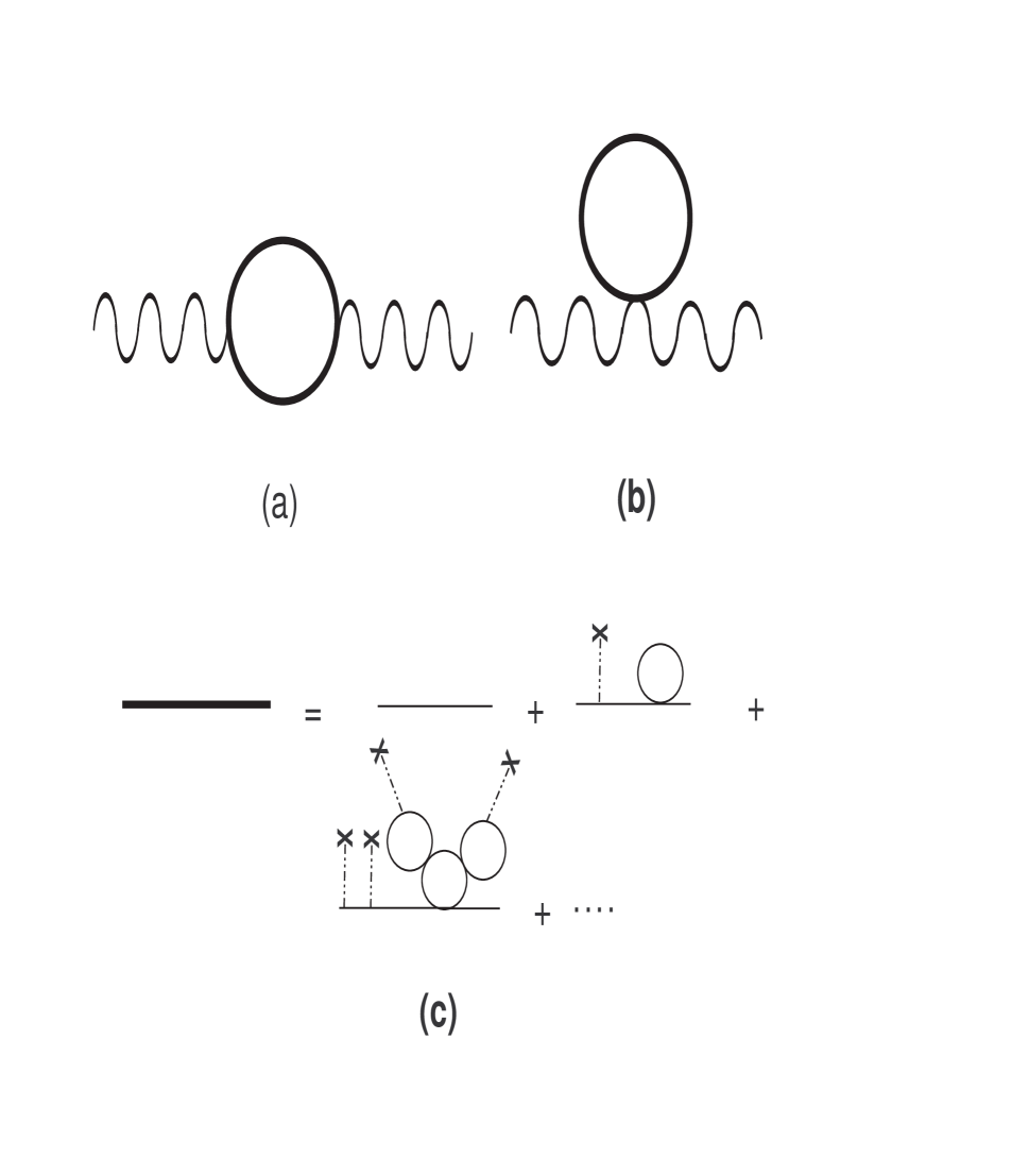
FIG. 3.: Photon polarization with full large $N$ scalar propagators. The dashed line with the cross at the end represents an insertion of the background $\eta(\tau)$.

FIG. 4.: Kinematical configuration corresponding to saddle point for photoproduction in the broken symmetry case

FIG. 5.: Kinematical configuration corresponding to saddle point for photoproduction in the unbroken symmetry case

FIG. 6.: Effective Magnetic Mass for $k=0$ as a function of time, Broken Symmetry, $g=10^{-4},\;\eta_{0}=0$

FIG. 7.: Effective Magnetic Mass for $k=0$ as a function of time, Unbroken Symmetry, $g=10^{-5},\;\eta_{0}=4$

FIG. 8.: $g\,q\,{\cal N}_{q}(\tau=2000)$ for the broken symmetry case as a function of $q$ for $g=10^{-4},\eta_{0}=0$. The distribution saturates for most of the range at $\tau\approx\tau_{NL}$ but for very small momentum.

FIG. 9.: $g\,q\,{\cal N}_{q}(\tau=500,1500,2000)$ for the unbroken symmetry case as a function of $q$ for $g=10^{-4}$. The distribution continues to evolve as a function of $\tau$. The peak at low momentum is at $q_{0}\approx\sqrt{\frac{K_{1}}{\tau}}$ and moves towards the origin while its magnitude increases.

FIG. 10.: The function $G(x)\equiv g\;q^{2}{\cal N}_{q}(\tau)$ as a function of $x\equiv q^{2}\tau$. Unbroken symmetry, $\eta_{0}=3,\;g=10^{-6}$

FIG. 11.: The integral $g\;\int_{0}^{\eta_{0}/\sqrt{2}}dq\;{\cal N}_{q}(\tau)/\omega_{q}$ that contributes to the Debye mass $m^{2}_{Deb}$ [see eq.(163)] as a function of $\tau$ for the unbroken symmetry case. The Debye mass grows with time as $\sqrt{\tau}$ as a result of the evolving distribution at small momemtum.

REFERENCES

- [1] J. W. Harris and B. Muller, Annu. Rev. Nucl. Part. Sci. 46, 71 (1996). B. Muller in Particle Production in Highly Excited Matter, Eds. H.H. Gutbrod and J. Rafelski, NATO ASI series B, vol. 303 (1993). H. Elze and U. Heinz, Phys. Rep. 183, 81 (1989); H. Meyer-Ortmanns, Rev. of Mod. Phys. 68, 473 (1996); H. Satz, in Proceedings of the Large Hadron Collider Workshop ed. G. Jarlskog and D. Rein, CERN, Geneva, Vol. 1. page 188; and in Particle Production in Highly Excited Matter, Eds. H.H. Gutbrod and J. Rafelski, NATO ASI series B, vol. 303 (1993).
- [2] B. Muller, The Physics of the Quark Gluon Plasma Lecture Notes in Physics, Vol. 225, Springer-Verlag, Berlin, Heidelberg, 1985; L. P. Csernai, ‘Introduction to Relativistic Heavy Ion Collisions’, John Wiley and Sons, England, 1994; C. Y. Wong, ‘Introduction to High-Energy Heavy Ion Collisions’, World Scientific, Singapore, 1994.
- [3] K. Geiger, Phys. Rep. 258, 237 (1995); Phys. Rev. D46, 4965 (1992) and D47, 133 (1993); Quark Gluon Plasma 2, Ed. by R. C. Hwa, World Scientific, Singapore, 1995.
- [4] X. N. Wang, Phys. Rep. 280, 287 (1997).
- [5] K. J. Eskola, Prog. Theor. Phys. Suppl. 129 (1997) 1; K. J. Eskola, K. Kajantie, P. V. Ruuskanen, Eur.Phys.J. C1 (1998) 627; K.J. Eskola, B. Müller, Xin-Nian Wang, Phys. Lett. B374 (1996) 20; K. J. Eskola, Nucl. Phys. A590 (1995) 383c.
- [6] J. Alam, S. Raha, B. Sinha, Phys. Rep., 273, 243 (1996).
- [7] D. Boyanovsky, H. J. de Vega, R. Holman and S. Prem Kumar, Phys. Rev. D56, 3929 and 5233 (1997).
- [8] For a discussion of a quenched chiral phase transition, see K. Rajagopal in Quark Gluon Plasma 2, Ed. by R. C. Hwa, World Scientific, Singapore, 1995; K. Rajagopal and F. Wilczek, Nucl. Phys. B379, 395 (1993) and Nucl. Phys. B404, 577 (1993).
- [9] for reviews of inflation, see R. Brandenberger, Rev. of Mod. Phys. 57, 1 (1985); Int. J. Mod. Phys. A2, 77 (1987); E. W. Kolb and M. S. Turner, The Early Universe, Addison Wesley, Redwood City, 1990 and A. Linde, Particle Physics and Inflationary Cosmology, Harwood Academic Publishers, Chur, Switzerland, 1990 and references therein.
- [10] See for example: P. J. E. Peebles, The Large Scale Structure of the Universe Princeton University Press, Princeton, NJ, 1980. Ya. B. Zel’dovich, A. A. Ruzmaikin and D. D. Sokoloff, Magnetic Fields in Astrophysics, Gordon and Breach, N.Y. 1983.
- [11] M. S. Turner and L. M. Widrow, Phys. Rev. D37, 2743 (1988).
- [12] G. Baym, D. Bödeker and L. Mclerran, Phys. Rev. D53, 662 (1996).
- [13] J. Ahonen and K. Enqvist, Phys. Rev. D57, 664 (1998).
- [14] K. Enqvist, in Strong and Electroweak Matter ’97, Ed. F. Csikor, Z. Fodor, World Scientific, Singapore, 1998. K. Enqvist and P. Olesen, Phys. Lett. B 329, 178 (1994).
- [15] J. M. Quashnock, A. Loeb and D. N. Spergel, Astrophys. J. 344, L49, (1989).
- [16] B. Cheng and A. Olinto, Phys. Rev. D50, 2421 (1994).
- [17] See for example the recent review by H. Satz, hep-ph/9908339; T. S. Biro, B. Müller and X.-N. Wang, Phys. Lett. B283, 171 (1992).
- [18] G. Baym, H. Monien, C. J. Pethick and D. G. Ravenhall, Phys. Rev. Lett. 64, 1867 (1990); E. Braaten and M. H. Thoma, Phys. Rev. D44, 1298 (1991).
- [19] R. D. Pisarski, Phys. Rev. Lett. 63, 1129 (1989); Phys. Rev. D47,5589 (1993).
- [20] A. Hosoya and K. Kajantie, Nucl. Phys. B250, 666 (1985); K. Enqvist, A. I. Rez and V. B. Semikoz, Nucl. Phys. B436, 49 (1995).
- [21] G. Baym and H. Heiselberg, Phys. Rev. D56, 5254 (1997).
- [22] U. Kraemmer, A. Rebhan, and H. Schulz, Ann. Phys. (N.Y.) 238, 286 (1995).
- [23] M.H. Thoma and C.T. Traxler, Phys. Lett. B378, 233 (1996); S. Leupold and M. H. Thoma, hep-ph/9908460.
- [24] J. Traschen and R. Brandenberger, Phys Rev D42, 2491 (1990); Y. Shtanov, J. Traschen and R. Brandenberger, Phys. Rev. D51, 5438 (1995). L. Kofman, A. Linde and A. Starobinsky, Phys. Rev. Lett. 73, 3195 (1994) and 76, 1011 (1996), Phys. Rev. D56 (1997) 3258.
- [25] D. Boyanovsky, H. J. de Vega, R. Holman, D.S-Lee and A. Singh, Phys. Rev. D51 (1995) 4419; D. Boyanovsky, D. Cormier, H. J. de Vega, R. Holman, A. Singh, M. Srednicki, Phys. Rev. D56 (1997) 1939; D. Boyanovsky, D. Cormier, H.J. de Vega and R. Holman, Phys. Rev D55, 3373 (1997); D. Boyanovsky, D. Cormier, H. J. de Vega, R. Holman and S. Prem Kumar, Phys. Rev. D57, 2166 (1998).
- [26] S. Mrowczynski and B. Muller, Phys. Lett. B363 (1995) 1.
- [27] U. Kraemmer, A.K.Rebhan, and H. Schulz, Ann. Phys. 238, 286 (1995).
- [28] D. Boyanovsky, H. J. de Vega, S. P. Kumar and R. Pisarski, Phys. Rev. D 58, 125009 (1998).
- [29] J. I. Kapusta, Finite Temperature Field Theory, Cambridge Monographs on Mathematical Physics, Cambridge Univ. Press, 1989.
- [30] E. Fradkin, Proc. Lebedev Phys. Inst. 29 (1965) 7.
- [31] M. Le Bellac, Thermal Field Theory, Cambridge University Press, 1996.
- [32] M. H. Thoma, in Quark Gluon Plasma 2, ed. by R. C. Hwa, World Scientific, Singapore, 1995.
- [33] J. Schwinger, J. Math. Phys. 2, 407 (1961); K. T. Mahanthappa, Phys. Rev. 126, 329 (1962); P. M. Bakshi and K. T. Mahanthappa, J. Math. Phys. 41, 12 (1963); L. V. Keldysh, JETP 20, 1018 (1965); K. Chou, Z. Su, B. Hao And L. Yu, Phys. Rep. 118, 1 (1985); A. Niemi and G. Semenoff, Ann. of Phys. (NY) 152, 105 (1984); N. P. Landsmann and C. G. van Weert, Phys. Rep. 145, 141 (1987); E. Calzetta and B. L. Hu, Phys. Rev. D41, 495 (1990) and D37, 2838 (1990); J. P. Paz, Phys. Rev. D41, 1054 (1990) and D42, 529(1990).
- [34] D. Boyanovsky and H. J. de Vega, Phys. Rev. D47, 2343 (1993). D. Boyanovsky, D.-S. Lee and A. Singh, Phys. Rev. D48, 800 (1993).
- [35] D. Boyanovsky, H. J. de Vega and R. Holman, Proceedings of the Second Paris Cosmology Colloquium, Observatoire de Paris, June 1994, pp. 127-215, H. J. de Vega and N. Sánchez, Editors, World Scientific, 1995; Advances in Astrofundamental Physics, Erice Chalonge Course, N. Sánchez and A. Zichichi Editors, World Scientific, 1995;
- [36] See for example: D. Boyanovsky, H. J. de Vega and R. Holman, p. 183-270 in the Proceedings of the Vth. Erice School ‘D. Chalonge’, ‘Current Topics in Astrofundamental Physics’, N. Sánchez and A. Zichichi, editors, World Scientific, 1997. D. Boyanovsky, D. Cormier, H. J. de Vega, R. Holman and S. Prem Kumar, Erice Chalonge School, Current Topics in Astrofundamental Physics, N. Sánchez and A. Zichichi Editors, p. 119-194, Kluwer, 1998 and references therein.
- [37] D. Boyanovsky, H. J. de Vega, R. Holman, J. F. J. Salgado, Phys. Rev. D54, 7570 (1996); D. Boyanovsky, C. Destri, H. J. de Vega, R. Holman and J. F. J. Salgado, Phys. Rev. D57, 7388 (1998); D. Boyanovsky, H. J. de Vega, R. Holman and J. F. J. Salgado, Phys. Rev. D59, 125009 (1999).
- [38] D. Boyanovsky, D. Brahm, R. Holman and D. S. Lee, Phys. Rev. D54, 1763 (1996).
- [39] D. Boyanovsky, H. de Vega and S.-Y. Wang, hep-ph/9909369.
- [40] F. Cooper, S. Habib, Y. Kluger, E. Mottola, J. P. Paz, P. R. Anderson, Phys. Rev. D50, 2848 (1994).
- [41] L. McLerran and T. Toimela, Phys. Rev. D31, 545 (1985).
- [42] P. V. Ruuskanen, in ‘Particle Production in Highly Excited Matter’, ed. H. Gutbrod, Plenum, N.Y.1993; Nucl.Phys. A 544, 169c (1995).
- [43] C. Gale and J. Kapusta, Phys. Rev. C 38, 2659 (1988).
- [44] J. Kapusta, P. Lichard and D. Seibert, Phys. Rev. D44, 2774 (1991).
- [45] R. Baier, S. Peigné and D. Schiff, Z. Phys. C62, 337 (1994). R. Baier, M. Dirks, K. Redlich and D. Schiff, Phys. Rev. D56, 2548 (1997).
- [46] D. Boyanovsky, H. J. de Vega, R. Holman and M. Simionato, Phys. Rev. D60, 065003 (1999). D. Boyanovsky and H. J. de Vega, Phys. Rev. D59, 105019 (1999).
- [47] D. Boyanovsky, I.D. Lawrie, D.S. Lee, Phys. Rev. D54, 4013, (1996).