BNL-HET-99/18

PLY-MS-99-23

Charges from Dressed Matter: Construction
Emili Bagan
Physics Dept.
Brookhaven National Laboratory
Upton, NY 11973
USA
Martin Lavelle, and David McMullan
School of Mathematics and Statistics
The University of Plymouth
Plymouth, PL4 8AA
UK

Abstract: There is a widespread belief in particle physics that there is no relativistic description of a charged particle. This is claimed to be due to persistent, long range interactions which distort the in and out going plane waves and generate infra-red divergences. In this paper we will show that this is not the case in QED. We construct locally gauge invariant charged fields which do create in and out Fock states. In a companion paper we demonstrate that the Green’s functions of these fields have a good pole structure describing particle propagation.

1 Introduction

The successes of hadronic physics are to a great extent based on our use of partonic variables in the ultraviolet (UV) domain. However, in the realm of soft physics, where the dynamics of quarks and gluons underlie jet formation and hadronisation, we simply do not know what variables to use. Strong interaction phenomenology could be a primary source of information here and this is, to a large extent, based upon effective quark models. However, the ‘quarks’ which compose these models are, although undoubtedly useful in very many ways, in no sense organic to Quantum Chromodynamics (QCD). This remains the case when such models are further mutated in the hope of making them more closely resemble the low energy dynamics of QCD, e.g., by introducing ‘gluons’ into effective quark models. Whatever these effective variables are, they are not simply the Lagrangian fields of QCD.

Knowledge of the correct infra-red (IR) variables in QCD would help us to obtain a deeper understanding of the structure of the underlying field theories of the standard model, to obtain some feeling for the validity and the (a priori unknown) limits of phenomenological models in particle physics and, most importantly, help us understand hadronisation and confinement. This paper is devoted to the construction of physical charged fields using only the gauge theories of the fundamental interactions. Faced with such a major task, we cannot hope to solve it immediately and our procedure will be essentially perturbative. Our aim is to develop methods and insight which may be carried over and extended into the non-perturbative domain. We intend to show below that this aim is not completely unrealistic.

Let us first recall how the problems associated with the use of unphysical variables show themselves in the standard description of scattering. In the LSZ approach it is assumed that at times long before or after any scattering process the fields entering or emerging from the vertex do not interact with each other any more. The experimental fact of hadronisation tells us that this cannot be true if our asymptotic fields are just taken to be the Lagrangian quark fields. Although we can describe the hadronisation process in one of the many models, this is necessarily matched on to partons emerging from the scattering process. This has even been elevated to the status of the principle of local parton hadron duality [1, 2]. However, this matching onto free partons has a price: quarks and gluons still interact with each other even when widely separated. The various IR divergences in on-shell Green s functions and in $S$-matrix elements are a direct consequence of the neglect of such interactions. In fact even in Quantum Electrodynamics (QED), where there is a $1/r$ fall-off in the interaction between the charges which we will generically refer to as electrons, it has long been known [3, 4, 5, 6, 7, 8, 9, 10] that this fall-off is still too slow to permit us to ignore the interaction and its neglect is responsible for the IR catastrophe.

There are various responses to this situation: the one most widely, if tacitly, employed has been to give up any description of on-shell Green s functions and $S$-matrix elements and to restrict oneself to IR safe quantities, such as, in QED, cross-sections summed over all final state soft photons. This response is at once theoretically radical (discarding the $S$-matrix) and practically conservative (we should only attempt to talk about this class of measurable quantities). It may be noted that this posture does not address the questions initially raised above, viz. what are the correct IR degrees of freedom? A second approach is to redefine the division of the Hamiltonian into free and interaction terms so that the new interaction can indeed be neglected at asymptotic times. This approach has been studied for QED by various authors [3, 8, 11, 12] but has not been successfully extended to QCD. As stressed by the authors of [8], taking this route entails the loss of a particle description already at the level of QED! (The perturbative signal for this is that the on-shell QED Green’s functions so obtained, although IR finite, do not have a pole structure describing particle propagation, rather the external lines for electrons and other charged fields have branch functions.) A third reaction, which we pursue below, is to argue that the experimentally observed particles entering and leaving scattering processes do not directly correspond to the variables which we have in the Lagrangian. E.g., when an electron emerges from a scattering process it is accompanied by an electromagnetic field which is not accounted for by the free Lagrangian fermion, $\psi$. We will refer to the inclusion of such fields as dressing the Lagrangian matter field. Such ideas have been investigated by many authors, see, e.g., [13, 14, 15, 16, 14, 17, 18, 19, 20, 21, 22, 23, 24, 25, 26, 27, 28].

We will argue below that this last approach, choosing the correct asymptotic fields, indeed solves the problem in a way which is compatible with having the expected pole structure, retaining the $S$-matrix and having a particle description. Here of course we need to understand what are the ‘correct’ fields. We will present below two requirements for the construction of such fields and further show how the descriptions which satisfy these conditions may be obtained in a systematic fashion which can be extended to other theories and which will permit the eventual inclusion of non-perturbative dynamics.

We have seen that the interaction in gauge theories cannot be neglected at large times. Now the Lagrangian fields in QED transform under gauge transformations as

$$A_{\mu}(x)\to A_{\mu}(x)+\partial_{\mu}\theta(x)\,,\qquad\mathrm{and}\qquad\psi(x)\to\mathrm{e}^{ie\theta(x)}\psi(x)\,,$$ (1)

so, since the coupling does not vanish, the matter field, $\psi$, is not gauge invariant at large times and cannot be identified with a physical particle such as an electron even in the asymptotic region. Can we then construct a gauge invariant charged field at all?

To make this more precise, we can use the tools of constrained dynamics (see, e.g., [29]). The prime requirement, as far as we are concerned in this paper, is that a physical field must satisfy Gauss’ law, which reads

$$\partial^{i}F_{i0}=-eJ_{0}\,.$$ (2)

Since Gauss’ law generates gauge transformations, this translates into the requirement of gauge invariance. There is a great deal of work in the literature on gauge invariant variables or simply variables with simplified gauge transformation properties, see, e.g., [30, 31, 32]. However, the identification of such variables with charged particles is especially subtle. The main point we wish to note here is that Gauss’ law tells us that charged matter fields cannot be separated from the electromagnetic cloud which surrounds them. This implies then that any description of a physical charged particle cannot be local since the total charge can always be written as a surface integral at spatial infinity [24]. We should also point out that, since the charge density generates global (rigid) gauge transformations, charged particles are not invariant under such gauge transformations.

The first construction of charged fields that we are aware of was performed by Dirac [13], who noted the existence of a set of composite fields

$$\psi_{f}(x)\equiv\exp\left(-ie\int\!d^{4}zf^{\mu}(x-z)A_{\mu}(z)\right)\psi(x)\,,$$ (3)

which, Dirac argued, are locally (but not globally) gauge invariant for any $f^{\mu}$ so long as $\partial_{\mu}f^{\mu}(w)=\delta^{(4)}(w)$ holds.

It is easy to see that there are many gauge invariant descriptions (many functions $f$ which fulfil this property). One of the main ideas behind the work reported here is that gauge invariance is not enough: a physical field must single itself out by further requirements. It is easy to see that some constructions are gauge invariant but highly unphysical: the most obvious example being the stringy ansatz

$$\psi_{\Gamma}(x)\equiv\exp\left(-ie\int_{\Gamma}^{x}dz_{i}A_{i}(x_{0},\boldsymbol{z})\right)\psi(x)\,,$$ (4)

which, it can be shown [28], corresponds to an infinitely excited state where the electric flux is confined along the path of the string, $\Gamma$. The reader can find an animation showing the decay of such a state at http://www.ifae.es/~roy/qed.html.

Dirac suggested the requirement that, out of the general set of functions given by Eq. 3, the physical description should have the correct electric field. Concretely, he noted that a physical charged particle is accompanied by an electric field and argued that an electron should be described by

$$\psi_{D}(x)\equiv\exp\left(-ie\frac{\partial_{i}A_{i}}{\nabla^{2}}\right)\psi(x)\,,$$ (5)

which is easily seen to be a special case of (3). His argument for this choice was that the state, $\psi_{D}(x)|0\rangle$, has a Coulombic electric field

$$E_{i}(x_{0},{\boldsymbol{x}})\psi_{D}(y)|0\rangle=-\frac{e}{4\pi}\frac{{\boldsymbol{x}_{i}-\boldsymbol{y}_{i}}}{|{\boldsymbol{x}-\boldsymbol{y}}|^{3}}\psi_{D}(y)|0\rangle\,.$$ (6)

To obtain this result, he used the equal-time commutator: $[E_{i}(x),A_{j}(y)]={i}\delta_{ij}\delta({\boldsymbol{x}}-{\boldsymbol{y}})$. We note that $\psi_{D}$ is locally gauge invariant and that the factor of $1/\nabla^{2}$ in (5) shows the non-locality of the electromagnetic cloud around the charge, since

$$\frac{1}{\nabla^{2}}f({\boldsymbol{x}})=-\frac{1}{4\pi}\int\!d^{3}x\frac{f({\boldsymbol{y}})}{|{{\boldsymbol{x}}-{\boldsymbol{y}}}|}\,.$$ (7)

Since no spatial direction is singled out, we might naively expect this to probably describe a static charge and this is in agreement with (6).

A natural question now is how we should interpret this gauge invariant field? Dirac argued that it corresponds to a charge at ${\boldsymbol{y}}$ together with its associated Coulombic electric field. Since the Coulomb field is that of a static charge, his interpretation implies that we know both the position and the velocity of the charge! This, as is well known from heavy quark effective theory (HQET), is only compatible with the uncertainty principle in the infinite mass limit. This will be clarified in Sect. 3 for charges with finite masses.

An obvious test of Dirac’s construction is to study whether these fields remove the IR singularities associated with on-shell static charges. The simplest test is the two-point function of charges described by (5) in an on-shell renormalisation scheme. It was shown in [33] that this is indeed IR finite so long as the static point on the mass shell is chosen, i.e., $p=(m,0,0,0)$. (The generalisation of this to the propagator at an arbitrary point on the mass shell was shown in [34] for scalar QED and in [35] for the fermionic theory.)

We note that it was further shown in [36] how to extend this description of dressed electrons to construct gauge invariant dressed quarks in non-abelian gauge theories at any order in perturbation theory (see the appendix of [24]). Essentially there is a minimal perturbative extension of the QED result which retains gauge invariance. We note that Haller and his collaborators [37, 38] have also obtained perturbative formulae which agree with this minimal extension of the static charge (5).

Three important implications of this work for QCD are that colour charges are only well defined [39] for locally gauge invariant fields such as our dressed quarks and gluons; the identification of a topological obstruction to the construction of an isolated quark [24] and the perturbative identification [40] of the dominant gluonic configuration responsible for asymptotic freedom.

In the rest of this paper we will present a method to construct charged particles in QED. We will systematically obtain explicit solutions and further demonstrate that the charged fields we construct, since they are surrounded by the correct electromagnetic fields, obey a free asymptotic dynamics. It will become clear that our results reflect previous work on the structure of the asymptotic dynamics which is found when it is assumed that the fields entering and leaving scattering processes are just the free matter fields, however, in our approach we will retain a particle interpretation.

In a companion paper [41], II, the results which we obtain below, and the interpretation which we give to them, will be further verified. In particular, we will use our physical variables and study the IR behaviour and UV properties of various Green’s functions and $S$-matrix elements.

The structure of this paper is then as follows. In Sect. 2 we discuss the asymptotic fields and dynamics of QED in some detail. Then, in Sect. 3, we show how to correctly characterise charges and construct static charges. The solution for a charge in QED with an arbitrary, relativistic velocity is presented in Sect. 4. In Sect. 5 the field theoretical implications of this approach are briefly reviewed and in Sect. 6 we present some conclusions and discuss the implications of this paper.

2 Dynamics and Asymptotic Dynamics

The starting point for our analysis of the physical, charged sector of QED is the familiar Lagrangian density

$${\cal L}=-{\textstyle\frac{1}{4}}F_{\mu\nu}F^{\mu\nu}+i\bar{\psi}\gamma^{\mu}(\partial_{\mu}-ieA_{\mu})\psi-m\bar{\psi}\psi+{\textstyle\frac{1}{2}}B^{2}+B\partial_{\mu}A^{\mu}\,.$$ (8)

Note that here we use Feynman gauge, $B=-\partial_{\mu}A^{\mu}$, for a discussion of other gauges, see, e.g., [42]. There is a significant algebraic advantage to working in this gauge which leads to a much simpler account of our construction of charges. We insist, though, that our fundamental variables (which will be introduced in the next section) are themselves gauge invariant and hence insensitive to this choice of the Feynman gauge. In the companion paper II, we will indeed see the gauge invariance of our construction in many perturbative calculations.

The extraction of the equal-time commutation relations from (8) is, at least, formally straightforward even in a fully interacting theory. What is much more difficult to do is to construct the general space-time commutators of these Heisenberg fields. For the $B$ field, though, things are much better since in Feynman gauge it satisfies the free equations of motion ($\Box B=0$). This fact, in conjunction with the known equal-time commutation relations, leads to the space-time commutators [43]:

$$[B(x),B(y)]=0\,,$$ (9)

$$[B(x),A_{\mu}(y)]=i\partial_{\mu}^{x}D(x-y)$$ (10)

and

$$[B(x),\psi(y)]=eD(x-y)\psi(y)\,.$$ (11)

where

$$D(x-y) = -\frac{1}{2\pi}\epsilon(x^{0}-y^{0})\delta((x-y)^{2})$$ (12)

$$= -\int\!\frac{d^{3}k}{(2\pi)^{3}}\;\frac{1}{\omega_{k}}e^{i{\boldsymbol{k}}{\cdot}({\boldsymbol{x}}-{\boldsymbol{y}})}\sin\Bigl{(}\omega_{k}(x^{0}-y^{0})\Bigr{)}\,,$$ (13)

and $\omega_{k}=|{\boldsymbol{k}}|$. We stress that these commutators are valid for all times and, in particular, hold both at very early and at very late times.

The significance of these commutation relations comes from the role of the $B$ field in characterizing the physical states and observables of the theory. Given its trivial dynamics, we can expand this field in terms of its modes:

$$B(x)=\int\!\frac{d^{3}k}{(2\pi)^{3}}\;\frac{1}{2\omega_{k}}\Bigl{\{}c(k)\mathrm{e}^{-ik{\cdot}x}+c^{\dagger}(k)\mathrm{e}^{ik{\cdot}x}\Bigr{\}}\,.$$ (14)

The condition on physical states is then that they are annihilated by the positive frequency part of $B$, i.e.,

$$c(k)|\mathrm{phys}\rangle=0\,,$$ (15)

for all $k$. Observables must preserve this condition, and hence must commute with $c(k)$. From the space-time commutators (10) and (11) we find that

$$[c(k),A_{\mu}(y)]=-ik_{\mu}\mathrm{e}^{ik{\cdot}y}\,$$ (16)

and

$$[c(k),\psi(y)]=-ie\,\mathrm{e}^{ik{\cdot}y}\psi(y)\,.$$ (17)

The first of these relations expresses the well known fact that not all components of the vector potential are physical: at the end of the day there should be just two physical photonic degrees of freedom per space-time point. In contrast, the second relation (17) is not usually interpreted as saying that the matter fields are unphysical. This is because this commutator contains an explicit dependence on the coupling constant. The widespread assumption then is that, in the remote past and future, the interaction vanishes and hence the asymptotic matter fields can be taken as physical. There is, though, no obvious reason why the large time limit of (17) should vanish. Indeed, the long range nature of the electromagnetic interaction suggests that it is highly unlikely that a non-interacting regime is ever reached. In fact these arguments are usually expressed [44] as an ad hoc assumption that the interaction is adiabatically switched off in the remote past and future.

The appeal to such a ‘switching off’  mechanism for the interaction does not reflect the experimental set-up found in a typical scattering process. Rather, what happens is that the in-coming, or out-going, particles become widely separated and that it is this growing separation that effectively renders the coupling to vanish. In theories with no more than cubic interactions (such as spinorial QED) there is a simple argument first used (to the best of our knowledge) by Kulish and Faddeev [8] to indicate that in theories with massless fields, this assumption is not true, i.e., the asymptotic dynamics in QED is not that of the free theory.

The idea is very simple: go into the interaction picture and take the large time limit of the interaction. If this limit is zero, then the asymptotic dynamics is that of a free theory. If the interaction does not vanish, then we simply cannot take the asymptotic dynamics to be free.

In QED this works as follows. The interaction Hamiltonian in the interaction picture is given by

$${H}_{\mathrm{int}}(t)=-e\int\!d^{3}x\;A^{\mathrm{f}}_{\mu}(t,{\boldsymbol{x}})J^{{\mathrm{f}}\,\mu}(t,{\boldsymbol{x}})\,,$$ (18)

where the free matter current is $J^{{\mathrm{f}}\,\mu}(t,{\boldsymbol{x}})=\bar{\psi}^{\mathrm{f}}(t,{\boldsymbol{x}})\gamma^{\mu}\psi^{\mathrm{f}}(t,{\boldsymbol{x}})$ and we are using the superscript ${\mathrm{f}}$ to distinguish the free fields from the corresponding interacting or Heisenberg ones. To further fix our notation, we take as our free field expansions

$$\psi^{\mathrm{f}}(x)=\int\!\frac{d^{3}p}{(2\pi)^{3}}\;\frac{1}{\sqrt{2E_{\smash{p}}}}\left\{b(p,s)u^{s}(p)e^{-ip{\cdot}x}+{d^{{\dagger}}}(p,s)v^{s}(p)e^{ip{\cdot}x}\right\}\,,$$ (19)

where $E_{p}=\sqrt{|{\boldsymbol{p}}|^{2}+m^{2}}$, a sum over $s$ is understood and

$$A^{\mathrm{f}}_{\mu}(x)=\int\!\frac{d^{3}k}{(2\pi)^{3}}\;\frac{1}{2\omega_{\smash{k}}}\left\{a_{\mu}(k)e^{-ik{\cdot}x}+{a^{{\dagger}}}_{\mu}(k)e^{ik{\cdot}x}\right\}\,.$$ (20)

We note here the basic space-time commutator for the free vector potential

$$[A^{\mathrm{f}}_{\mu}(x),A^{\mathrm{f}}_{\nu}(y)]=-ig_{\mu\nu}D(x-y)\,.$$ (21)

Inserting these free field expansions directly into (18) results in eight terms which can be grouped according to the positive and negative frequency components of the fields. Each of these pieces will have a time dependence of the form $e^{i\psi t}$ where $\psi$ involves sums and differences of energy terms. The argument used in [8] (see also [10] and the discussion in supplement S4 of [46]) is that, as $t$ tends to plus or minus infinity, only terms with $\psi$ tending to zero can survive and thus contribute to the asymptotic interaction. After performing the spatial integration, and using the resulting momentum delta function, one finds that in a theory describing massive charges only four terms of the form $\psi=\pm(E_{p+k}-E_{p}\pm\omega_{k})$ can survive in the large time limit. The requirement that $E_{p+k}-E_{p}\pm\omega_{k}\approx 0$ can only be met in QED because the photon is massless, in which case it implies that $\omega_{k}\approx 0$, i.e., only the infra-red regime contributes to the asymptotic dynamics. From this observation it can be shown [8, 45] that the full interacting Hamiltonian (18) does not vanish asymptotically, but has in fact the same asymptotic limit as

$${H}_{\mathrm{int}}^{{\mathrm{as}}}(t)=-e\int\!d^{3}x\;A^{\mathrm{f}}_{\mu}(t,{\boldsymbol{x}})J^{\mu}_{{\mathrm{as}}}(t,{\boldsymbol{x}})$$ (22)

with

$$J^{\mu}_{{\mathrm{as}}}(t,{\boldsymbol{x}})=\int\!\frac{d^{3}p}{(2\pi)^{3}}\;\frac{p^{\mu}}{E_{p}}\rho(p)\delta^{3}\bigl{(}{\boldsymbol{x}}-t{\boldsymbol{p}}/E_{p}\bigr{)}\,.$$ (23)

The operators in this current are only contained in the charge density

$$\rho(p)=\sum_{s}\Bigl{(}{b^{{\dagger}}}(p,s)b(p,s)-{d^{{\dagger}}}(p,s)d(p,s)\Bigr{)}$$ (24)

which implies that the asymptotic current satisfies the trivial space-time commutator relation

$$[J^{\mu}_{\mathrm{as}}(x),J^{\nu}_{\mathrm{as}}(y)]=0\,.$$ (25)

As such, this asymptotic current can be interpreted as effectively the integral over all momenta of the current associated with a charged particle moving with velocity ${\boldsymbol{p}}/E_{p}$. This does not vanish as $t\to\infty$. We thus see that the asymptotic dynamics of QED is not that of a free theory.

It is important to note here that by ‘asymptotic dynamics’ we are referring to the dynamics in the neighbourhood of time-like and null boundaries of Minkowski space-time. At space-like infinity things are very different: the fields vanish and we impose the condition that the local gauge transformations become the identity there. This distinction is made clear in the Penrose diagram [47] of Figure 1.

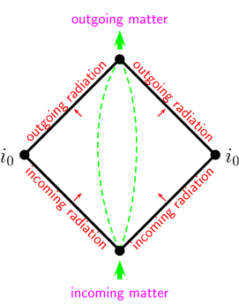
Figure 1: Penrose diagram of Minkowski space-time: the dashed lines are the worldlines of massive particles while the short arrows depict incoming and outgoing radiation. We may only demand that fields vanish at space-like infinity, $i_{0}$.

What this argument has shown us is that, contrary to the statements found in the usual approaches to scattering in QED, the basic commutator (11) really does imply that the matter field is not physical even in the asymptotic regime. The Lagrangian fermion in QED should not be associated with anything physical such as an electron! So what can we identify with physical matter?

Given that we are dealing with a gauge theory with an unbroken symmetry, so that the reduction in the degrees of freedom must be in the gauge sector of the theory, it is clear [48] that we cannot now try to reduce the degrees of freedom in the matter sector. Rather, a procedure is needed for finding a gauge invariant combination of both matter and gauge fields — we call this general process dressing the matter fields. This will be the topic of the next section. Before moving on to that construction, though, it is useful to continue our previous analysis of the asymptotic form of the matter and gauge fields.

It is important to realise that there are two clear steps in the extraction of the asymptotic form of the fields entering into our theory.

• First we go from the Heisenberg fields to the interacting fields via the usual time ordered exponential of the interacting Hamiltonian:

  $$O_{\mathrm{I}}(t,t_{0})=T\exp\left(-i\!\!\int_{t_{0}}^{t}\!d\tau\,{H}_{\mathrm{int}}(\tau)\right)O_{\mathrm{H}}(t)\,\widetilde{T}\exp\left(i\!\!\int_{t_{0}}^{t}\!d\tau\,{H}_{\mathrm{int}}(\tau)\right)\,,$$ (26)

  where $T$ and $\widetilde{T}$ signify time and anti-time ordering respectively. This transformation requires the introduction of an arbitrary time $t_{0}$ at which the fields in the two pictures agree. This time is arbitrary at this stage because if we were to directly transform back to the Heisenberg fields all reference to $t_{0}$ would vanish. At lowest order in the coupling we find that the relation between a Heisenberg operator $O_{\mathrm{H}}(t)$ and its interaction picture counterpart is

  $$O_{\mathrm{I}}(t,t_{0})=O_{\mathrm{H}}(t)-i\int_{t_{0}}^{t}d\tau\,[{H}_{\mathrm{int}}(\tau),O_{\mathrm{H}}(t)]\,.$$ (27)

• The asymptotic dynamics for the Heisenberg fields is now found by using the asymptotic form of the interaction Hamiltonian to translate from the interaction to the Heisenberg picture. At lowest order in the coupling we get

  $$O_{\mathrm{H}}^{\mathrm{as}}(t,t_{0}) = O_{\mathrm{I}}(t,t_{0})+i\int_{t_{0}}^{t}d\tau\,[{H}_{\mathrm{int}}^{\mathrm{as}}(\tau),O_{\mathrm{I}}(t,t_{0})]$$ (28)

  $$= O_{\mathrm{H}}(t)+i\int_{t_{0}}^{t}d\tau\,[{H}_{\mathrm{int}}^{\mathrm{as}}(\tau)-{H}_{\mathrm{int}}(\tau),O_{\mathrm{H}}(t)]\,.$$

Note that there is a $t_{0}$ dependence in this expression for the asymptotic fields at time $t$ due to the potential contribution from the lower range of integration. This dependence is governed by the value of ${H}_{\mathrm{int}}^{\mathrm{as}}(t_{0})-{H}_{\mathrm{int}}(t_{0})$, so if we set $t_{0}=\pm\infty$ this will vanish by the construction of the asymptotic interaction.

In practice, though, we do not want to start in the Heisenberg picture, rather we wish to go directly from the known fields in the interaction picture. What this argument then tells us is that we are free to ignore any explicit contributions from the overlap time $t_{0}$ as long as this is taken to be large.

The transformation from the interaction picture to the asymptotic Heisenberg picture is implemented by the usual time ordered product of the Hamiltonian (22). Using the commutator relations (25) and (21), this can be written as the product of two commuting terms:

$$T\exp\!\!\left(i\!\!\int_{-\infty}^{t}\!\!\!\!\!\!d\tau\,{H}_{\mathrm{int}}^{{\mathrm{as}}}(\tau)\right)=\exp\!\!\left(i\!\!\int_{-\infty}^{t}\!\!\!\!\!\!d\tau\,{H}_{\mathrm{int}}^{{\mathrm{as}}}(\tau)\right)\exp\!\!\left({\textstyle\frac{1}{2}}\!\!\int_{-\infty}^{t}\!\!\!\!\!\!d\tau_{1}\int_{-\infty}^{\tau_{1}}\!\!\!\!\!\!d\tau_{2}\,[{H}_{\mathrm{int}}^{{\mathrm{as}}}(\tau_{1}),{H}_{\mathrm{int}}^{{\mathrm{as}}}(\tau_{2})]\right)\,.$$ (29)

From (25) and (21), the double commutator $[[{H}_{\mathrm{int}}^{{\mathrm{as}}}(\tau_{1}),{H}_{\mathrm{int}}^{{\mathrm{as}}}(\tau_{2})],A^{\mathrm{f}}(x)]=0$, and hence the asymptotic vector potential is given by ($t=x^{0}$)

$$A^{\mathrm{as}}_{\mu}(x) = \exp\!\!\left(i\!\!\int_{-\infty}^{t}\!\!\!\!\!\!d\tau\,{H}_{\mathrm{int}}^{{\mathrm{as}}}(\tau)\right)A^{\mathrm{f}}_{\mu}(x)\exp\!\!\left(-i\!\!\int_{-\infty}^{t}\!\!\!\!\!\!d\tau\,{H}_{\mathrm{int}}^{{\mathrm{as}}}(\tau)\right)$$ (30)

$$= A^{\mathrm{f}}_{\mu}(x)-e\int_{-\infty}^{t}\!\!d\tau d^{3}y\,D(\tau-t,{\boldsymbol{y}}-{\boldsymbol{x}})J^{\mathrm{as}}_{\mu}(\tau,{\boldsymbol{y}})\,.$$

Note that it follows from this that

$$\Box A^{\mathrm{as}}_{\mu}(x)=-eJ^{\mathrm{as}}_{\mu}(x)\,,$$ (31)

and hence we see that the asymptotic vector potential is made from a free part plus the field generated by the non-trivial asymptotic current, i.e., a response to the presence of any other charges. We also have from (21) and (25) that the asymptotic fields obey the same commutator as the free fields

$$[A^{\mathrm{as}}_{\mu}(x),A^{\mathrm{as}}_{\nu}(y)]=-ig_{\mu\nu}D(x-y)\,.$$ (32)

The asymptotic form of the matter field follows in much the same way, but now both terms in (29) contribute. The resulting field is [8]

$$\psi^{\mathrm{as}}(x)=\int\!\frac{d^{3}p}{(2\pi)^{3}}\;\frac{1}{\sqrt{2E_{\smash{p}}}}D(p,t)\left\{b(p,s)u^{s}(p)e^{-ip{\cdot}x}+{d^{{\dagger}}}(p,s)v^{s}(p)e^{ip{\cdot}x}\right\}$$ (33)

where the distortion operator $D(p,t)$ factors into two commuting terms (reflecting the similar factorisation in (29)): $D(p,t)=D_{{\mathrm{phase}}}(p,t)D_{{\mathrm{soft}}}(p,t)$. The phase component $D_{{\mathrm{phase}}}(p,t)$ does not depend on the gauge field (it is in fact gauge invariant) and only contributes to the phase of the operator (see the discussion in Supplement S4 of [46]), as such we will neglect its contribution to the asymptotic field. We do note, though, that this phase depends on the presence of other charges in the system and hence enters into the distortion operator only at order $e^{2}$ and above in the coupling.

The soft component of the distortion operator is given by

$$D_{{\mathrm{soft}}}(p,t)=\exp\left\{-e\!\!\!\int\limits_{{\mathrm{soft}}}\!\frac{d^{3}k}{(2\pi)^{3}}\;\frac{1}{2\omega_{k}}\left(\frac{p\cdot a(k)}{p\cdot k}\mathrm{e}^{-itk{\cdot}p/E_{p}}-\frac{p\cdot{a^{{\dagger}}}(k)}{p\cdot k}\mathrm{e}^{itk{\cdot}p/E_{p}}\right)\right\}\,,$$ (34)

where we have made explicit that only the soft (infra-red) regime contributes to the asymptotic fields. Due to this distortion operator, the asymptotic field $\psi^{\mathrm{as}}$ does not create or annihilate particle states. That is, if we were to define (as we would want to in the LSZ-reduction of the $S$-matrix) the operator

$$b(q,s,t):=\int\!d^{3}x\;\frac{1}{\sqrt{2E_{\smash{q}}}}u^{{\dagger}s}(q)\psi^{\mathrm{as}}(x)\mathrm{e}^{iq{\cdot}x}\,,$$ (35)

then rather than recovering the time independent, one particle annihilation operator, we get (neglecting the phase)

$$b(q,s,t)=D_{\mathrm{soft}}(q,t)b(q,s)\,.$$ (36)

This operator does not have a single particle like interpretation, indeed it does not even act in a Fock space as it is a coherent state operator. The perturbative expression of this is the infra-red problem in QED: one cannot extract poles from the on-shell Green’s functions of the theory and hence an $S$-matrix cannot be constructed [11, 49]. Such observations have led to the view among theorists [8] that no particle description is possible for the electron. Our point of view on this is that the matter field is simply not physical and we should not be shocked if its asymptotic limit is also unphysical: it is far too early to give up on the electron as a particle!

In order to identify just what does describe the physics in the asymptotic regime we minimally need to find fields which commute with the $B$ field. To this end we observe that at early and late times the $B$ field can be written solely in terms of the free electro-magnetic potential:

$$B(x)\to-\partial^{\mu}A^{\mathrm{as}}_{\mu}(x)=-\partial^{\mu}A^{\mathrm{f}}_{\mu}(x)\,.$$ (37)

This result follows from (30), and the conservation of the asymptotic current if

$$\lim_{a\to\infty}\int\!d^{3}y\;\frac{1}{|y|}\delta(a-|y|)J_{0}^{\mathrm{as}}(a,y)=0\,.$$ (38)

To demonstrate this, we insert the explicit expression (23) for the asymptotic current into (38). This generates a product of delta functions whose arguments, it can be immediately seen, cannot both vanish for massive matter fields.

Hence the modes of the $B$-field responsible for identifying the physical states (15) are asymptotically given by the modes of the free vector potential as

$$c(k)=ik\cdot a(k)\,.$$ (39)

Thus, the modes of the free fermionic field (19) are physical in the asymptotic regime. Hence ${d^{{\dagger}}}(q,s)|0\rangle$ is indeed an asymptotic, charged one-particle state. But it is not the asymptotic limit of the Lagrangian matter field. Given that this charged state is created by a free creation operator, one might now ask if it indeed has an associated electromagnetic field. The important point to note is that the asymptotic potential (30) is not that of a free theory. In particular, using (12) and (30), we see that

$$[A^{\mathrm{as}}_{\mu}(x),{d^{{\dagger}}}(q,s)]=-\frac{e}{4\pi}\frac{q_{\mu}}{\sqrt{(q\cdot x)^{2}-q^{2}x^{2}}}{d^{{\dagger}}}(q,s)\,.$$ (40)

We recall from Chap. 14 of [50] that the classical electro-magnetic potential associated with a charge moving with momentum $q$ is, at large distances, given by

$$A_{\mu}^{\mathrm{class}}(x)=-\frac{e}{4\pi}\frac{q_{\mu}}{\sqrt{(q\cdot x)^{2}-q^{2}x^{2}}}\,.$$ (41)

Thus the electromagnetic potential associated with the state ${d^{{\dagger}}}(q,s)|0\rangle$ indeed corresponds, at large distances, to that of a particle moving with momentum $q$. Hence the asymptotically physical operator ${d^{{\dagger}}}(q,s)$ creates both a charged particle state with momentum $q$ and its associated electromagnetic potential.

To summarise: we have seen that ${d^{{\dagger}}}(q,s)$ is physical and creates the correct electromagnetic field expected for a moving charge. It is, however, not directly related to the the asymptotic limit of the matter field $\psi$. Is there then a (gauge invariant) operator which has ${d^{{\dagger}}}(q,s)$ as its asymptotic limit? This is an important question since if there is such a field, then this would correspond asymptotically to an electron. The construction of such a field will be the subject of the next section.

3 Static Charges

We have seen that it is indeed possible to construct gauge invariant, charged particle states at asymptotic times in QED. In fact, these states are elements of the familiar Fock space associated with the modes of the free fermionic field. In this sense, QED is no different from any other theory with purely massive fields. Where QED differs from other (non-gauge) theories is in the fact that these fields are not the asymptotic limits of the matter fields from which the Lagrangian of the theory was constructed. The neglect of this simple fact generates the infra-red problem, prevents the construction of $S$-matrix elements and leads to the abandonment of a particle description of charges. In order to motivate our general construction of the fields which do asymptotically correspond to the charged particle states, we will, in this section, reanalyse Dirac’s construction of the static charged field and show in what sense it correctly describes a static charged particle.

Dirac’s construction of the field $\psi_{D}$ raises many fundamental questions that we need to address if we are to make progress in our aim to describe charged fields in both QED and, more generally, in the standard model. For example, it is far from clear how unique this construction is or how it should be extended to a non-abelian theory such as QCD where the chromo-electric field of a static charge is not known a priori.

Before analysing the uniqueness of the construction, let us first of all see how a static interpretation of $\psi_{D}$ emerges even when the fields are not infinitely massive. To this end we define the gauge invariant annihilation operator $b(q,s,t,0)$ by

$$b(q,s,t,0):=\int\!d^{3}x\;\frac{1}{\sqrt{2E_{\smash{q}}}}u^{{\dagger}s}(q)\exp\bigg{(}-ie\frac{\partial_{i}A_{i}}{\nabla^{2}}\bigg{)}(x)\psi(x)\mathrm{e}^{iq{\cdot}x}\,.$$ (42)

The momentum $q$ is taken to be on-shell in this definition. The additional label ‘0’ in this operator reflects the conjectured static nature of Dirac’s construction.

At $O(e)$, the proposed annihilation operator (42) is the sum of two terms, one from the matter as seen in Sect. 2 and one coming from the expansion of the dressing:

$$b^{[1]}(q,s,t,0)=\int\!d^{3}x\;\frac{1}{\sqrt{2E_{\smash{q}}}}u^{{\dagger}s}(q)\psi(x)\mathrm{e}^{iq{\cdot}x}-ie\int\!d^{3}x\;\frac{1}{\sqrt{2E_{\smash{q}}}}u^{{\dagger}s}(q)\frac{\partial_{i}A_{i}}{\nabla^{2}}(x)\psi(x)\mathrm{e}^{iq{\cdot}x}\,,$$ (43)

where the superscript signifies that we only retain terms up to order $e$. Starting in the interaction picture, then transforming to the asymptotic Heisenberg picture will result in the first term in (43) becoming the $O(e)$ distorted annihilation operator (36). Given that the second term in (43) is already at $O(e)$, its asymptotic limit in this approximation will simply be the large time limit of the operator expressed in terms of the free fields (19) and (20). Using the identity

$$\frac{\partial_{i}A^{\mathrm{f}}_{i}}{\nabla^{2}}(x)=i\int\!\frac{d^{3}k}{(2\pi)^{3}}\;\frac{1}{2\omega_{k}}\bigg{(}\frac{{\boldsymbol{k}}\cdot{\boldsymbol{a}}(k)}{{\boldsymbol{k}}^{2}}\mathrm{e}^{-ik{\cdot}x}-\frac{{\boldsymbol{k}}\cdot{\boldsymbol{a}}^{\dagger}(k)}{{\boldsymbol{k}}^{2}}\mathrm{e}^{ik{\cdot}x}\bigg{)}\,,$$ (44)

and the Kulish-Faddeev argument discussed in Sect. 2, the second term in (43) can be shown to have the asymptotic form

$$eb(q,s)\int\limits_{{\mathrm{soft}}}\!\frac{d^{3}k}{(2\pi)^{3}}\;\frac{1}{2\omega_{k}}\bigg{(}\frac{{\boldsymbol{k}}\cdot{\boldsymbol{a}}(k)}{{\boldsymbol{k}}^{2}}\mathrm{e}^{-itk{\cdot}q/E_{q}}-\frac{{\boldsymbol{k}}\cdot{\boldsymbol{a}}^{\dagger}(k)}{{\boldsymbol{k}}^{2}}\mathrm{e}^{itk{\cdot}q/E_{q}}\bigg{)}\,.$$ (45)

Combining the two contributions to $b^{[1]}(q,s,t,0)$, we get, in the large time limit, the modified distorted annihilation operator

$$b^{[1]}(q,s,t,0)\to b(q,s)\Bigg{\{}1+ \!\!\!\!\!\!\!\!e\int\limits_{{\mathrm{soft}}}\!\frac{d^{3}k}{(2\pi)^{3}}\;\frac{1}{2\omega_{k}}\bigg{[}\bigg{(}\frac{{\boldsymbol{k}}\cdot{\boldsymbol{a}}(k)}{{\boldsymbol{k}}^{2}}-\frac{q\cdot a(k)}{q\cdot k}\bigg{)}\mathrm{e}^{-itk{\cdot}q/E_{q}}$$ (46)

$$\qquad-\bigg{(}\frac{{\boldsymbol{k}}\cdot{\boldsymbol{a}}^{\dagger}(k)}{{\boldsymbol{k}}^{2}}-\frac{q\cdot a^{\dagger}(k)}{q\cdot k}\bigg{)}\mathrm{e}^{itk{\cdot}q/E_{q}}\bigg{]}\Bigg{\}}\,.$$

In general this distortion does not vanish and thus, even though we are dealing with a gauge invariant field, it does not allow for a charged particle interpretation. However, if the 4-momentum $q$ is at the static point in the mass-shell, i.e., when the four-momentum $q^{\mu}$ is $m\eta^{\mu}$, where $\eta$ is the unit temporal vector, then the distortion terms are

$$-e\int\limits_{{\mathrm{soft}}}\!\frac{d^{3}k}{(2\pi)^{3}}\;\frac{1}{2\omega_{k}}\bigg{(}\frac{k\cdot a(k)}{{\boldsymbol{k}}^{2}}\mathrm{e}^{-it\omega_{k}}\!\!\!\!\!\!\!\!\! -\frac{k\cdot a^{\dagger}(k)}{{\boldsymbol{k}}^{2}}\mathrm{e}^{it\omega_{k}}\bigg{)}$$ (47)

$$=e\int\limits_{{\mathrm{soft}}}\!\frac{d^{3}k}{(2\pi)^{3}}\;\frac{i}{2\omega^{3}_{k}}(c(k)\mathrm{e}^{-it\omega_{k}}+c^{\dagger}(k)\mathrm{e}^{it\omega_{k}})\,,$$

where we have used the asymptotic identification (39) of the modes of the $B$ field. As we have seen, these modes commute with the free annihilation operator $b(q,s)$ and with themselves. Hence, using the definition of physical states, (15), we see that between physical states the distortion operator reduces to the identity operator at the static point in the mass shell.

The above analysis shows that matter dressed à la Dirac, $\psi_{D}$, has a particle interpretation. This interpretation we stress only holds at the static point in the mass shell. Before discussing the exponentiation of this result, or indeed its extension to moving charges, we need to understand the uniqueness of the construction. To this end, we need to step back and ask where this solution came from, i.e., how should we characterise the dressing so that it describes a charged particle with a well defined velocity?

Let us initially look at the simpler situation where we have a heavy matter field, $\varphi(x)$. This field can be thought of as the infinite mass limit of either a scalar or Dirac field which is, for the moment, not coupled to a gauge theory. In this limit velocity is superselected [51] and the equation of motion for the field has the universal form

$$u\cdot\partial\varphi(x)=0\,,$$ (48)

where $u$ is the associated 4-velocity of the heavy particle. This equation is simply the statement that the field is constant along the world line of a particle moving with 4-velocity $u$. Indeed, if we parameterise the world line of a particle moving with 4-velocity $u^{\mu}=\gamma(\eta+v)^{\mu}$ (where $\eta$ is the unit time-like vector introduced above, $v=(0,{\boldsymbol{v}})$ is the velocity and $\gamma=(1-|{\boldsymbol{v}}|^{2})^{-1/2}$) as

$$x^{\mu}(s)=x^{\mu}+(s-x^{0})(\eta+v)^{\mu}\,,$$ (49)

then (48) implies that for arbitrary $s$,

$$\varphi(x(s))=\varphi(x(0))\,.$$ (50)

If the heavy matter field is now minimally coupled then the equation of motion (48) becomes

$$u\cdot D\varphi(x)=0\,,$$ (51)

where $D_{\mu}=\partial_{\mu}-ieA_{\mu}$. There is now no heavy charged particle interpretation to this equation. However the field $\varphi$ should not, and indeed cannot, be identified as a physical field since it is not gauge invariant. The lack of a simple particle interpretation to the field $\varphi$ is thus not a serious problem since what we need to do first is to dress this field. We will demand that the dressing is such that, in addition to restoring gauge invariance, it should also ensure that a (heavy) particle interpretation for the dressed matter field holds.

We define the gauge invariant charged matter field by

$$\Phi(x)=h^{-1}(x)\varphi(x)\,,$$ (52)

where the dressing $h^{-1}(x)$ is such that under a gauge transformation we have

$$h^{-1}(x)\to h^{-1}(x)\mathrm{e}^{-ie\theta(x)}\,.$$ (53)

That is, a physical particle corresponds to the heavy matter field dressed with some ‘brown muck’, whose exact form we will now clarify. For this field to correspond to a heavy charged particle we must have $u\cdot\partial\Phi=0$. This follows from (51) if the dressing satisfies

$$u\cdot\partial h^{-1}(x)=-ieh^{-1}(x)u\cdot A(x)\,.$$ (54)

We call this equation the dressing equation. Equations (53) and (54) are the fundamental requirements on any description of charged particles and are central to what follows.

Although our motivation for this equation emerged from an analysis of the heavy matter sector, we demand that, more generally, it holds for the dressing of any field that is asymptotically corresponding to a charged particle moving with velocity $u$. There are two arguments for this: it is well known that the asymptotic dynamics of QED is governed by soft photons for whom any electron is heavy; secondly, it can be shown[10] that the asymptotic interaction Hamiltonian vanishes for the propagator of the dressed fields which satisfy (54) if one is at the right point in the mass-shell. We now specialise to the static situation and leave the general case to the next section.

In the static situation the dressing equation (54) becomes

$$\partial_{0}h^{-1}(x)=-ieh^{-1}(x)A_{0}(x)\,.$$ (55)

The first thing to note about this is that Dirac’s proposal (5) does not satisfy this equation! Indeed, using the identity

$$\partial_{\mu}\mathrm{e}^{O}=\mathrm{e}^{O}\big{(}\partial_{\mu}O+{\textstyle\frac{1}{2}}[\partial_{\mu}O,O]\big{)}$$ (56)

where $O$ is an arbitrary operator whose commutator $[\partial_{\mu}O,O]$ is a c-number, we find that

$$\partial_{0}\exp\bigg{(}-ie\frac{\partial_{i}A_{i}}{\nabla^{2}}(x)\bigg{)}=-ie\exp\bigg{(}-ie\frac{\partial_{i}A_{i}}{\nabla^{2}}(x)\bigg{)}\Bigg{(}\frac{\partial_{0}\partial_{j}A_{j}}{\nabla^{2}}(x)+\frac{e}{2}\int\!\frac{d^{3}k}{(2\pi)^{3}}\;\frac{1}{\omega_{k}^{2}}\Bigg{)}\,,$$ (57)

and even if we ignore the field independent term in the last factor, we do not solve (55).

To understand the relationship between Dirac’s dressing and the static version of the dressing equation we need to solve equation (55). As is well known, the solution to equations like (55) have the form of an anti-time ordered exponential:

$$h^{-1}(x,a)\approx\widetilde{T}\exp\bigg{(}-ie\int_{a}^{t}A_{0}(s,{\boldsymbol{x}})\,ds\bigg{)}\,,$$ (58)

where $a$ is, as yet, undetermined. Although this clearly solves (55), it does not satisfy the gauge transformation property (53) which is essential for a dressing. Indeed, under a gauge transformation we have

$$h^{-1}(x,a)\to\mathrm{e}^{ie\theta(a,{\boldsymbol{x}})}h^{-1}(x,a)\mathrm{e}^{-ie\theta(x)}\,.$$ (59)

There is no choice for the parameter $a$ for which $\theta(a,{\boldsymbol{x}})$ vanishes (the choice $a=\pm\infty$ evaluates $\theta$ at time-like infinity where there are no restrictions on the gauge transformations, see Fig. 1).

We can compensate for this bad behaviour under gauge transformations, while still solving the dressing equation (55), by taking instead

$$h^{-1}(x,a)=\exp\bigg{(}-ie\frac{\partial_{i}A_{i}}{\nabla^{2}}(a,{\boldsymbol{x}})\bigg{)}\widetilde{T}\exp\bigg{(}-ie\int_{a}^{t}A_{0}(s,{\boldsymbol{x}})\,ds\bigg{)}\,.$$ (60)

This we can write as

$$h^{-1}(x,a)=\widetilde{T}\exp\bigg{(}-ie\int_{a}^{t}\Big{\{}A_{0}(s,{\boldsymbol{x}})-\frac{\partial_{0}\partial_{i}A_{i}}{\nabla^{2}}(s,{\boldsymbol{x}})\Big{\}}\,ds\bigg{)}\exp\bigg{(}-ie\frac{\partial_{i}A_{i}}{\nabla^{2}}(x)\bigg{)}\,,$$ (61)

where we have combined the two exponentials of (60) under one exponential, then written one part as a total derivative. We have neglected, for the moment, possible commutator terms which will be discussed in Sect. 4. The first term in this expression is now gauge invariant, a fact which becomes manifest when we write this solution as

$$h^{-1}(x,a)=\widetilde{T}\exp\bigg{(}ie\int_{a}^{t}\frac{\partial^{\mu}F_{\mu 0}}{\nabla^{2}}(s,{\boldsymbol{x}})\,ds\bigg{)}\exp\bigg{(}-ie\frac{\partial_{i}A_{i}}{\nabla^{2}}(x)\bigg{)}\,.$$ (62)

Thus we see a factorisation of the static dressing into a minimal part which is essential for gauge invariance (and is just Dirac’s original proposal for the static dressing), plus an additional part which is separately gauge invariant.

This general solution to the static dressing equation takes on a much simpler form in the asymptotic regime where a charged particle picture should emerge. Using the asymptotic space-time commutators (32) we see that

$$[\partial^{\mu}F^{\mathrm{as}}_{\mu\nu}(x),F^{\mathrm{as}}_{\lambda\rho}(y)]=0\,.$$ (63)

This commutator implies two important results. Firstly, the additional part of the dressing will commute with the electric and magnetic field operators, and thus the electromagnetic field associated with the static dressing is the same as that produced by the minimal, Dirac component. Hence we see that Dirac’s argument for the form of the dressing was not sensitive enough to detect the additional term. Secondly, we can use this commutator to dispense with the anti-time ordering in the dressing (62) so that in the asymptotic regime

$$h^{-1}(x,a)\to\exp\bigg{(}ie\int_{a}^{t}\frac{\partial^{\mu}F^{\mathrm{as}}_{\mu 0}}{\nabla^{2}}(s,{\boldsymbol{x}})\,ds\bigg{)}\exp\bigg{(}-ie\frac{\partial_{i}A^{\mathrm{as}}_{i}}{\nabla^{2}}(x)\bigg{)}\,.$$ (64)

Using Gauss’ law (2) in the asymptotic domain, and the identification (30), we see that the static dressing factorises in the asymptotic regime into the product of two terms. One can be made out of the various matter contributions and is gauge invariant, it is analogous to the phase term in the distortion operator for the matter field. The other part of the dressing is constructed out of the free vector potential and, for reasons that will become immediately apparent, we call it the soft part of the dressing:

$$h^{-1}_{\mathrm{soft}}(x)=\exp\bigg{(}-ie\frac{\partial_{i}A^{\mathrm{f}}_{i}}{\nabla^{2}}(x)\bigg{)}\,.$$ (65)

This is the most important component in QED and, as was shown in [40], its extension to QCD is the dominant glue around quarks at short distances.

Armed with this result, we can now study the exponentiation of the soft contributions to the asymptotic annihilation operator (42). Repeating the Kulish-Faddeev argument for the soft components of both the matter and dressing we find that

$$b(q,s,t,0)\to h^{-1}_{\mathrm{soft}}(q,t)D_{\mathrm{soft}}(q,t)b(q,s)\,,$$ (66)

where

$$h^{-1}_{{\mathrm{soft}}}(q,t)=\exp\!\!\Bigg{\{}e\!\!\int\limits_{{\mathrm{soft}}}\!\frac{d^{3}k}{(2\pi)^{3}}\;\frac{1}{2\omega_{k}}\bigg{(}\frac{{\boldsymbol{k}}\cdot{\boldsymbol{a}}(k)}{{\boldsymbol{k}}^{2}}\mathrm{e}^{-itk{\cdot}q/E_{q}}-\frac{{\boldsymbol{k}}\cdot{\boldsymbol{a}}^{\dagger}(k)}{{\boldsymbol{k}}^{2}}\mathrm{e}^{itk{\cdot}q/E_{q}}\bigg{)}\Bigg{\}}\,,$$ (67)

which is the exponentiation of our previous result (45). The combined effect of these distortion factors can easily be evaluated using the canonical commutation relations for the modes $a_{\mu}(k)$ and the Baker-Campbell-Hausdorff formula. One finds

$$h^{-1}_{\mathrm{soft}}(q,t)D_{{\mathrm{soft}}}(q,t) = \exp\Bigg{\{}e\!\!\int\limits_{{\mathrm{soft}}}\!\frac{d^{3}k}{(2\pi)^{3}}\;\frac{1}{2\omega_{k}}\bigg{[}\bigg{(}\frac{{\boldsymbol{k}}\cdot{\boldsymbol{a}}(k)}{{\boldsymbol{k}}^{2}}-\frac{q\cdot a(k)}{q\cdot k}\bigg{)}\mathrm{e}^{-itk{\cdot}q/E_{q}}$$ (68)

$$\qquad\qquad\qquad-\bigg{(}\frac{{\boldsymbol{k}}\cdot{\boldsymbol{a}}^{\dagger}(k)}{{\boldsymbol{k}}^{2}}-\frac{q\cdot{a^{{\dagger}}}(k)}{q\cdot k}\bigg{)}\mathrm{e}^{itk{\cdot}q/E_{q}}\bigg{]}\Bigg{\}}\,.$$

Note that the commutator in the BCH-formula vanishes here. Just as we saw in (47), this becomes the identity operator between physical states at the correct point in the mass-shell where the momentum $q^{\mu}$ is at the static point in the mass shell: $q^{\mu}=m\eta^{\mu}$.

To summarise: we have seen in this section how to characterise the dressing appropriate to a charged particle moving with a given velocity. In the static case we solved the dressing equation and saw how Dirac’s proposal for a static charge emerged as the minimal part of the static dressing. Using this construction we showed how the static annihilation operator emerges as the asymptotic limit of the statically dressed matter field. Having seen how to describe static charges, we now proceed to an analysis of moving charges.

4 Moving Charges

In this section we will show that the dressing needed to describe a charged particle moving with four-velocity $u^{\mu}$ is

$$h^{-1}(x)=\mathrm{e}^{-ieK(x)}\mathrm{e}^{-ie\chi(x)}\,,$$ (69)

where the minimal part of the dressing is given by

$$\chi(x)=\frac{{\cal G}\cdot A}{{\cal G}\cdot\partial}\,,$$ (70)

with ${\cal G}^{\mu}=(\eta+v)^{\mu}(\eta-v)\cdot\partial-\partial^{\mu}$, and the additional (gauge invariant) part of the dressing is

$$K(x)=\int_{\pm\infty}^{x^{0}}(\eta+v)^{\mu}\frac{\partial^{\nu}F_{\nu\mu}}{{\cal G}\cdot\partial}(x(s))\,ds\,.$$ (71)

In this last expression the integral is along the world-line of a massive particle with four-velocity $u^{\mu}$ parameterised as in (49). Before deriving this result from the dressing equation (54), we will first verify that this dressing generates the correct electric and magnetic fields and demonstrate that its modes have the asymptotic limit appropriate to a charged particle moving with velocity ${\boldsymbol{v}}$.

In the asymptotic regime we can again argue from (63) that the additional component of the dressing does not affect the electromagnetic configuration. This allows us to define the minimally dressed charged field $\psi_{v}$ by

$$\psi_{v}(x)=\mathrm{e}^{-ie\chi(x)}\psi(x)\,.$$ (72)

By construction, this is gauge invariant. It is also straightforward to see that this field is physical in the context of the $B$-field formalism discussed in Sect. 2. In particular, from (16) and (17), it is easy to see that

$$[c(k),\psi_{v}(x)]=0\,.$$ (73)

In the static limit this dressed field reduces to Dirac’s expression (5), i.e., $\psi_{0}=\psi_{D}$.

Repeating the argument given by Dirac leading up to the expression (6) for the electric field of the static charge, the electromagnetic fields generated by (72) are given by the equal-time commutators $-ie[E_{i}(x),\chi(y)]_{{}_{\mathrm{et}}}$ and $-ie[B_{i}(x),\chi(y)]_{{}_{\mathrm{et}}}$. In order to evaluate these we first need to make clear how $1/{\cal G}\cdot\partial$ is defined in (70).

We take

$$\frac{1}{{\cal G}\cdot\partial}f({\boldsymbol{x}}):=\int\!d^{3}z\;G({\boldsymbol{x}}-{\boldsymbol{z}})f({\boldsymbol{z}})\,,$$ (74)

where

$${\cal G}\cdot\partial G({\boldsymbol{x}}-{\boldsymbol{z}})=\delta^{3}({\boldsymbol{x}}-{\boldsymbol{z}})$$ (75)

and we note from its definition that ${\cal G}\cdot\partial=\nabla^{2}-({\boldsymbol{v}}\cdot\partial)^{2}$. Taking the Fourier transform of (75) we see that

$$G({\boldsymbol{x}})=-\int\!\frac{d^{3}k}{(2\pi)^{3}}\;\frac{1}{{\boldsymbol{k}}^{2}-({\boldsymbol{v}}\cdot{\boldsymbol{k}})^{2}}e^{i{\boldsymbol{k}}{\cdot}{\boldsymbol{x}}}\,.$$ (76)

This integral is computed in the standard fashion by first diagonalising the quadratic form in the denominator. The final expression for $G({\boldsymbol{x}})$ is then

$$G({\boldsymbol{x}})=-\frac{1}{4\pi}\frac{\gamma}{\sqrt{{\boldsymbol{x}}^{2}+\gamma^{2}({\boldsymbol{v}}\cdot{\boldsymbol{x}})^{2}}}\,.$$ (77)

Note that in the static limit this reproduces (7).

The electric and magnetic fields generated by this dressing are now straightforward to calculate. For example, applying the operator (72) to a state $|0\rangle$ with no electric field, we find

$$E_{i}(x)\psi_{v}(y)|0\rangle=-\frac{e}{4\pi}\frac{\gamma({\boldsymbol{x}}-{\boldsymbol{y}})_{i}}{\big{(}|{\boldsymbol{x}}-{\boldsymbol{y}}|^{2}+\gamma^{2}({\boldsymbol{v}}\cdot({\boldsymbol{x}}-{\boldsymbol{y}}))^{2}\big{)}^{\frac{3}{2}}}\psi_{v}(y)|0\rangle\,.$$ (78)

This is precisely the electric field associated with a charged particle moving with velocity ${\boldsymbol{v}}$.

As we saw with the static charge, the interpretation of the operator $\psi_{v}(x)$ as that creating a moving charge at the point $x$ only holds in the infinite mass limit. More generally then, we extend the definition of the static, gauge invariant annihilation operator (42) to the moving case by defining the mode

$$b(q,s,t,v)=\int\!d^{3}x\;\frac{1}{\sqrt{2E_{\smash{q}}}}u^{{\dagger}s}(q)\exp\bigg{(}-ie\frac{{\cal G}\cdot A}{{\cal G}\cdot\partial}\bigg{)}(x)\psi(x)\mathrm{e}^{iq{\cdot}x}\,.$$ (79)

We will now demonstrate that this is a particle annihilation operator at the right point in the mass-shell.

At $O(e)$, $b^{[1]}(q,s,t,v)$ is the sum of two terms in which the free field expansions for the potential in the dressing can be used. Using the expression

$$\frac{{\cal G}\cdot A^{\mathrm{f}}}{{\cal G}\cdot\partial}(x)=i\int\!\frac{d^{3}k}{(2\pi)^{3}}\;\frac{1}{2\omega_{k}}\bigg{(}\frac{V\cdot a(k)}{V\cdot k}\mathrm{e}^{-ik{\cdot}x}-\frac{V\cdot a^{\dagger}(k)}{V\cdot k}\mathrm{e}^{ik{\cdot}x}\bigg{)}\,,$$ (80)

where we have introduced the notation that

$$V^{\mu}=(\eta+v)^{\mu}(\eta-v)\cdot k-k^{\mu}\,,$$ (81)

we see that in the large time limit

$$b^{[1]}(q,s,t,v)\to b(q,s)\Bigg{\{}1+ \!\!\!\!\!\!\!\!e\int\!\frac{d^{3}k}{(2\pi)^{3}}\;\frac{1}{2\omega_{k}}\bigg{[}\bigg{(}\frac{V\cdot a(k)}{V\cdot k}-\frac{q\cdot a(k)}{q\cdot k}\bigg{)}\mathrm{e}^{-itk{\cdot}q/E_{q}}$$ (82)

$$\qquad-\bigg{(}\frac{V\cdot a^{\dagger}(k)}{V\cdot k}-\frac{q\cdot a^{\dagger}(k)}{q\cdot k}\bigg{)}\mathrm{e}^{itk{\cdot}q/E_{q}}\bigg{]}\Bigg{\}}\,.$$

In the distortion term we note that we can write (recall that $k$ is on-shell)

$$\frac{V^{\mu}}{V\cdot k}-\frac{q^{\mu}}{q\cdot k} = \frac{(\eta+v)^{\mu}(\eta-v)\cdot k-k^{\mu}}{(\eta+v)\cdot k(\eta-v)\cdot k}-\frac{q^{\mu}}{q\cdot k}$$ (83)

$$= \frac{(\eta+v)^{\mu}}{(\eta+v)\cdot k}-\frac{q^{\mu}}{q\cdot k}-\frac{k^{\mu}}{V\cdot k}\,.$$

Hence, at the point in the mass-shell where $q^{\mu}=m\gamma(\eta+v)^{\mu}$, the distortion operator becomes the trivial operator

$$-e\int\!\frac{d^{3}k}{(2\pi)^{3}}\;\frac{1}{2\omega_{k}}\bigg{(}\frac{k\cdot a(k)}{V\cdot k}\mathrm{e}^{-it\omega_{k}}\!\!\!\!\!\!\!\!\! -\frac{k\cdot a^{\dagger}(k)}{V\cdot k}\mathrm{e}^{it\omega_{k}}\bigg{)}$$ (84)

$$=e\int\!\frac{d^{3}k}{(2\pi)^{3}}\;\frac{i}{2\omega_{k}V\cdot k}(c(k)\mathrm{e}^{-it\omega_{k}}+c^{\dagger}(k)\mathrm{e}^{it\omega_{k}})\,,$$

which vanishes between physical states.

The exponentiation of this result for the soft contributions to both the distortion operator and the dressing, follows in much the same way as it did for the static case. Indeed, at large times we get

$$b(q,s,t,v)\to h_{\mathrm{soft}}(q,t,v)D_{\mathrm{soft}}(q,t)b(q,s)\,,$$ (85)

where $D_{\mathrm{soft}}(q,t)$ is given in (34) and

$$h_{{\mathrm{soft}}}(q,t,v)=\exp\left\{e\!\!\!\int\limits_{{\mathrm{soft}}}\!\frac{d^{3}k}{(2\pi)^{3}}\;\frac{1}{2\omega_{k}}\left(\frac{V\cdot a(k)}{V\cdot k}\mathrm{e}^{-itk{\cdot}q/E_{q}}-\frac{V\cdot{a^{{\dagger}}}(k)}{V\cdot k}\mathrm{e}^{itk{\cdot}q/E_{q}}\right)\right\}\,.$$ (86)

The combined effect of these distortions yields the overall soft distortion of the particle mode as

$$h_{\mathrm{soft}}(q,t,v)D_{{\mathrm{soft}}}(q,t) = \exp\Bigg{(}e\!\!\int\limits_{{\mathrm{soft}}}\!\frac{d^{3}k}{(2\pi)^{3}}\;\frac{1}{2\omega_{k}}\bigg{[}\bigg{(}\frac{V\cdot a(k)}{V\cdot k}-\frac{q\cdot a(k)}{q\cdot k}\bigg{)}\mathrm{e}^{-itk{\cdot}q/E_{q}}$$ (87)

$$\qquad\qquad\qquad-\bigg{(}\frac{V\cdot{a^{{\dagger}}}(k)}{V\cdot k}-\frac{q\cdot{a^{{\dagger}}}(k)}{q\cdot k}\bigg{)}\mathrm{e}^{itk{\cdot}q/E_{q}}\bigg{]}\Bigg{)}\,.$$

Just as we saw above, this becomes the identity operator between physical states at that point in the mass-shell where $q^{\mu}=m\gamma(\eta+v)^{\mu}$.

This analysis has shown that the dressed matter $\psi_{v}$ can be interpreted as a charged particle moving with velocity $v$ at the appropriate point in the mass shell. In this sense, we see that a relativistic description of charged particle is indeed possible. This dressing (69) for a moving charge can, of course, be derived from the dressing equation (54). Full details of this are given in the appendix.

5 From Dressed Matter to the $S$-Matrix

In this section we want to show how the $S$-matrix elements of QED can be extracted in terms of Green’s functions of dressed matter fields. We will see that the usual perturbative techniques can be applied. It should become clear that a correct application of the usual LSZ formalism (for a discussion with fermionic fields see, e.g., Chap. 5 of Ref. [52]) requires the use of dressed matter.

Recall that in the usual LSZ route to the $S$-matrix it is assumed that there is an overlap at large times between the interacting fields and the free fields. This is schematically illustrated in Fig. 2. Since we have seen that this overlap does not take place between the usual matter fields in the QED Lagrangian, it is clear that we should expect problems in implementing the LSZ procedure and, indeed, one finds that the usual Green’s functions do not have a good pole structure. The responses to this range from using coherent states and abandoning the pole structure [53]) to giving up the idea of $S$-matrix elements and only considering inclusive cross-sections including all possible final state photons. We now want to show how the use of dressed fields in QED lets us follow the LSZ path to the $S$-matrix. The companion paper, II, will show in perturbative studies that good pole structures are obtained with the use of these fields.

Figure 2: Sketch of a scattering process where the coupling is assumed to vanish for large times.

Consider the simplest case: one particle goes to one particle. The equivalent $S$-matrix element may be expressed as

$$\langle\hbox{out}|{\hbox{in}}\rangle=\langle\hbox{out}|b^{{\dagger}}(q)|0\rangle\,,$$ (88)

where $|0\rangle$ is the vacuum state and $b^{{\dagger}}$ ($b$) are just the traditional one-particle Fock creation (annihilation) operators. In the free theory we may express the creation operator by

$$b^{{\dagger}}(q)=\int\!d^{3}x\;\frac{1}{2E_{q}}\psi^{{\dagger}}(x)u(q)\hbox{e}^{-iq\cdot x}\,.$$ (89)

Now it is normally assumed that for large times the usual Heisenberg fields approach the free fields. However, we have seen in Sect. 2 that this is not the case in unbroken gauge theories like QED. Rather, as was demonstrated in Sect.’s 3 and 4, we have at each point, $q$, on the mass shell an appropriately dressed field, $\psi_{v}$, such that in (89) we may, if we neglect the unobservable phase effects, (weakly) replace $\psi_{v}\to\psi^{f}$ for $t\to\pm\infty$. (Note that for simplicity we do not explicitly insert renormalisation constants. Renormalisation will be studied in the explicit calculations of II.)

We thus see that in QED we obtain

$$\langle\hbox{out}|b^{{\dagger}}(q)|0\rangle=\lim_{t\to-\infty}\int\!d^{3}x\;\frac{1}{2E_{q}}\langle\hbox{out}|\psi^{{\dagger}}_{v}(x)|0\rangle u(q)\hbox{e}^{-iq\cdot x}\,.$$ (90)

In the standard fashion we may introduce an integration over time to obtain

$$\langle\hbox{out}|b^{{\dagger}}(q)|0\rangle = -\int\!d^{4}x\frac{d}{dt}\frac{1}{2E_{q}}\langle\hbox{out}|\psi^{{\dagger}}_{v}(x)|0\rangle u(q)\hbox{e}^{-iq\cdot x}$$ (91)

$$\qquad+\lim_{t\to\infty}\int\!d^{3}x\;\frac{1}{2E_{q}}\langle\hbox{out}|\psi^{{\dagger}}_{v}(x)|0\rangle u(q)\hbox{e}^{-iq\cdot x}\,.$$

As is usual this second, reduced term corresponds to disconnected graphs and may be dropped.

The time derivative acts upon both the matter field and the exponential. Writing $\psi^{{\dagger}}_{v}=\bar{\psi}_{v}\gamma_{0}$ and using that $(q\!\!\!/-m)u(q)=0$, we find

$$\langle\hbox{out}|b^{{\dagger}}(q)|0\rangle=i\int\!d^{4}x\langle\hbox{out}|\bar{\psi}_{v}(x)|0\rangle(i{\overleftarrow{\not\!\partial}}+m)\frac{1}{2E_{q}}u(q)\hbox{e}^{-iq\cdot x}\,.$$ (92)

We note that this is the standard result, but the matter field is replaced by the appropriate dressed matter.

We now want to continue by using an annihilation operator to replace the out state by the vacuum. using the counterpart of (89), and taking time-ordering into account, we rapidly find

$$\langle\hbox{out}|{\hbox{in}}\rangle = \langle 0|b(p)b^{{\dagger}}(q)|0\rangle$$ (93)

$$= \int\!d^{4}x\int\!d^{4}y(i{{\not\!\partial}}_{y}-m)\langle 0|T\left(\psi_{v^{\prime}}(y)\bar{\psi}_{v}(x)\right)|0\rangle(i{\overleftarrow{\not\!\partial}}_{x}+m)$$

$$\qquad\qquad\qquad\quad\times\frac{1}{2E_{q}}u(q)\hbox{e}^{-iq\cdot x}\frac{1}{2E_{p}}u(p)\hbox{e}^{ip\cdot y}\,,$$

where $p$ (and $v^{\prime}$) correspond to the momentum (velocity) of the outgoing charge. Clearly this can be generalised to more interesting $S$-matrix elements.

We now want to reexpress (93) in terms of a Gell-Mann–Low formula. The usual method relies upon the existence of a unitary operation linking the Heisenberg and the free fields. We have already seen in this paper that the free matter fields are not unitarily related to the equivalent Heisenberg fields, but for the dressed fields we indeed have

$$\psi_{v}(t,{\boldsymbol{x}})=U^{-1}(t)\psi_{v}^{\rm f}(t,{\boldsymbol{x}})U(t)\,,$$ (94)

where $U$ is the usual operator, made up from exponentiating the interaction Hamiltonian expressed in terms of free fields. We stress that this relation only holds at the right point on the mass shell appropriate to the dressing.

Once we have this relation it is straightforward to repeat the usual procedure to obtain the standard Gell-Mann–Low formula but with the charged matter fields replaced everywhere by appropriately dressed matter. With this, we are in a position to perform perturbative tests. These are presented in the companion paper, II.

6 Conclusions

In this paper we have shown how to describe charged particles in relativistic QED through a process of dressing the matter with the appropriate electromagnetic cloud. The essential ingredients which we used to obtain the precise structure of the dressing were gauge invariance (53) and the kinematical requirement which we call the dressing equation (54).

We solved these two conditions and obtained a structured dressing composed of two factors: a minimal component which had the correct gauge transformation properties and an additional, gauge invariant part which was necessary to fulfill the dressing equation. In this paper we have focused primarily on the minimal part of the dressing and, in particular, we have shown that it removes the soft distortion factor which has been previously claimed to prevent a particle interpretation of QED. This has been demonstrated for a charged particle moving with an arbitrary velocity.

The vanishing of the distortion factor shows that the long range interactions of QED, due to the masslessness of the photon, are encoded in the dressing rather than any residual interaction term in the Hamiltonian. An important consequence of this is that the asymptotic Hamiltonian becomes the free Hamiltonian for our dressed fields. This means that the LSZ-formalism can be directly carried out without any use of a dubious adiabatic ‘switching off’ of the QED coupling.

The process of dressing a gauge dependent variable so as to make it gauge invariant is a very general procedure. How one would want to dress the fields that form a bound state might be very different from how individual charges should be dressed. In this work we are only interested in dressing a charged field so that it corresponds to a charged particle moving with the appropriate velocity at either early or late times. The interesting topic of how to describe, say, a bound state such as positronium, that is either entering or leaving a scattering process, we leave to future work.

Turning to QCD, where we want to construct colour charged quarks and gluons, we note first that our two fundamental requirements on the dressing have immediate non-abelian extensions. A simple algorithm for constructing the minimal, soft gluonic dressing around a quark can be found in [24]. The potential between two so-dressed quarks was studied in [40]. There it was shown that this dressing generates the anti-screening interaction of QCD which is responsible for asymptotic freedom. We have thus identified the non-abelian extension of the soft dressing as the dominant glue around quarks. A corollary of this result is that we see that the anti-screening interaction takes place between two separately gauge invariant constituent quarks and there is as yet no sign of any flux tube formation.

In the companion paper II we will take the results of this paper and submit them to a battery of tests. There we will see that the particle of our dressed fields also emerges from perturbative calculations. The Green’s functions of these fields will be shown to be free of on-shell infra-red divergences and to have the pole structure expected of physical particles. Detailed studies of the ultra-violet behaviour of these fields and their Green’s functions will be presented and it will be shown that the renormalisation programme can be carried out without difficulties.

Acknowledgements: This work was supported by the British Council/Spanish Education Ministry Acciones Integradas grant no.  1801 /HB1997-0141. We thank Robin Horan, Tom Steele, Shogo Tanimura and Izumi Tsutsui for discussions, the organisers of the XIXth UK Theory Institute where some of this work was carried out and PPARC for support from the Theory Travel Fund. EB thanks the HEP group at BNL for their warm hospitality and many interesting comments. He also acknowledges a grant from the Dirección General de Enseñanza Superior e Investigación Científica.

Appendix A Appendix

In this appendix we show how the dressing for a moving charge (69) follows directly from the gauge transformation properties (53) of the dressing and the dressing equation (54).

Before presenting the solution, we need to briefly reexamine Dirac’s general formula (3) for a gauge invariant field. In line with (3), we take as an ansatz for the electro-magnetic cloud an exponential of the form $\exp(-ie\chi(x))$ where, under a gauge transformation

$$\chi(x)\to\chi(x)+\theta(x)\,.$$ (95)

This is precisely the type of transformation that Dirac investigated in (3) and we would be tempted to accept as the general solution

$$\chi(x)=\int\!d^{4}z\,f^{\mu}(x-z)A_{\mu}(z)\,,$$ (96)

where $f^{\mu}(x-z)$ satisfies $\partial_{\mu}f^{\mu}(x-z)=\delta^{4}(x-z)$. But this only implies (95) if no surface terms arise when we integrate by parts. The restriction on the local gauge transformations to those that vanish at spatial infinity is quite natural as finite energy restrictions impose a $1/r$ fall-off on the potential. However, as discussed around Fig. 1, no such restriction applies to the fields at temporal infinity. Thus, to maintain gauge invariance, the form of $f^{\mu}(x-z)$ must be such that no surface terms arise at large times.

As it stands, we can only infer from this that $f^{0}(x-z)$ should be zero outside of some bounded region in the $z^{0}$-direction. To get more from this, we follow Dirac’s proposal for the static charge and take

$$\chi(x)=\int\!d^{4}z\,G(x-z){\cal G}^{\mu}A_{\mu}(z)\,,$$ (97)

where ${\cal G}^{\mu}$ is a first order, differential operator and ${\cal G}\cdot\partial\,G(x-z)=\delta^{4}(x-z)$. In order to avoid the surface terms that would obstruct the gauge transformation properties of the dressing, we must have that the operator ${\cal G}\cdot\partial$ cannot involve any time derivatives. Given this restriction, we see that $G(x-z)=\delta(x^{0}-z^{0})G({\boldsymbol{x}}-{\boldsymbol{z}})$ where

$${\cal G}\cdot\partial\,G({\boldsymbol{x}}-{\boldsymbol{z}})=\delta^{3}({\boldsymbol{x}}-{\boldsymbol{z}})\,.$$ (98)

We shall, for convenience, write $\chi$ as

$$\chi(x)=\int\!d^{3}z\,G({\boldsymbol{x}}-{\boldsymbol{z}})\,{\cal G}^{\mu}A_{\mu}(x_{0},{\boldsymbol{z}}):=\frac{{\cal G}\cdot A}{{\cal G}\cdot\partial}(x)\,,$$ (99)

which mirrors the notation adopted in the body of this paper (cf. Sect. 4). So far, of course, ${\cal G}$ remains undefined here.

We now make a more general ansatz, based upon our experience in the static case, i.e., that the dressing factorises into the product of two terms:

$$h^{-1}(x)=e^{-ieK(x)}e^{-ie\chi(x)}\,,$$ (100)

where $K$ is gauge invariant and $\chi\to\chi+\theta$ under the gauge transformation (1). The second term is thus a minimal part of the dressing, essential for the gauge transformation properties of the dressing. The first term in (100) is then an additional part of the dressing. Here we write this as a simple exponential, rather than a path-ordered exponential as we did for the static example in (58), since we are taking our fields to be the asymptotic fields discussed in Sect. 2, and the commutators of these fields will be seen to allow this ansatz. We note that all of the fields in the rest of this appendix are asymptotic fields and we omit the ‘as’ superscript in what follows.

For the additional part of the dressing it is enough in this abelian theory to also take $K$ to be linear in the fields and we find that it is sufficient to make the expansion

$$eK(x)=eK_{1}(x)+e^{2}K_{2}(x)\,.$$ (101)

The dressing equation (54) can then be expanded in powers of the coupling to give the two equations:

$$(\eta+v)^{\mu}\partial_{\mu}(K_{1}+\chi)=(\eta+v)^{\mu}A_{\mu}\,,$$ (102)

and

$$i(\eta+v)^{\mu}\partial_{\mu}K_{2}={\textstyle\frac{1}{2}}(\eta+v)^{\mu}\big{(}\partial_{\mu}[\chi,K_{1}]-[A_{\mu},K_{1}+\chi]\big{)}\,.$$ (103)

The solution to (102) is

$$K_{1}(x)+\chi(x)=\int_{a}^{x^{0}}(\eta+v)^{\mu}A_{\mu}(x(s))\,ds+\chi(x(a))\,,$$ (104)

where the integral is along the world line parameterised by (49) with starting point $a$. The constant term $\chi(x(a))$ is needed to ensure that $K$ is gauge invariant. This means that we can write $K_{1}$ in the manifestly invariant form:

$$K_{1}(x) = \int_{a}^{x^{0}}(\eta+v)^{\mu}\Big{(}A_{\mu}(x(s))-\partial_{\mu}\chi(x(s))\Big{)}\,ds$$ (105)

$$= \int_{a}^{x^{0}}(\eta+v)^{\mu}\frac{{\cal G}^{\nu}F_{\nu\mu}}{{\cal G}\cdot\partial}(x(s))\,ds\,.$$

The lower range of integration found in $K_{1}$ should, in this asymptotic regime, have no physical significance. This will be ensured if the derivative of the additional part of the dressing with respect to $a$ is zero between physical states. This would be the case if this derivative either vanishes or is constructed from the $B$-field. From the form of (105) we see that it will not vanish. Therefore we must show that it is made from the $B$-field. We thus postulate that it can be written as

$$\frac{\partial\ }{\partial a}K(x) = (\eta+v)^{\mu}\Big{(}\frac{\partial^{\nu}F_{\nu\mu}}{{\cal G}\cdot\partial}(x(a))+e\frac{J_{\mu}}{{\cal G}\cdot\partial}(x(a))\Big{)}\,,$$ (106)

$$= (\eta+v)^{\mu}\frac{\partial_{\mu}B}{{\cal G}\cdot\partial}(x(a))\,.$$

We now investigate what this implies for $K_{1}$ and $K_{2}$.

From equations (105) and (106) we see that

$$\frac{\partial\ }{\partial a}K_{1}(x) = -(\eta+v)^{\mu}\frac{{\cal G}^{\nu}F_{\nu\mu}}{{\cal G}\cdot\partial}(x(a))$$ (107)

$$= (\eta+v)^{\mu}\frac{\partial^{\nu}F_{\nu\mu}}{{\cal G}\cdot\partial}(x(a))\,.$$

Hence, from the anti-symmetry of $F_{\nu\mu}$ and the fact that ${\cal G}^{\nu}$ is a first order differential operator constructed out of $\partial^{\nu}$, $\eta^{\nu}$ and $v^{\nu}$, we must have that

$${\cal G}^{\nu}=-\partial^{\nu}+(\eta+v)^{\nu}(\alpha\eta\cdot\partial+\beta v\cdot\partial)\,.$$ (108)

The constants $\alpha$ and $\beta$ can be fixed by the requirement that ${\cal G}\cdot\partial$ contains no time derivatives. It is easy to see that

$${\cal G}\cdot\partial=(\alpha-1)(\eta\cdot\partial)^{2}+(\alpha+\beta)(\eta\cdot\partial)(v\cdot\partial)+\beta(v\cdot\partial)^{2}+\nabla^{2}\,.$$ (109)

Hence we must have that $\alpha=1$ and $\beta=-1$. From this we see that

$${\cal G}^{\nu}=(\eta+v)^{\nu}(\eta-v)\cdot\partial-\partial^{\nu}\,.$$ (110)

Given this result we obtain

$$K_{1}(x)=\int_{a}^{x^{0}}(\eta+v)^{\mu}\frac{\partial^{\nu}F_{\nu\mu}}{{\cal G}\cdot\partial}(x(s))\,ds\,.$$ (111)

Using the commutators (63) it follows that

$$[K_{1}(x),\frac{\partial K_{1}}{\partial a}(x)]=0\,$$ (112)

and hence the $a$-independence of the construction will follow from (106) if

$$\frac{\partial K_{2}}{\partial a}(x)=(\eta+v)^{\nu}\frac{J_{\nu}}{{\cal G}\cdot\partial}(x(a))\,.$$ (113)

This equation and (103) determine the form of $K_{2}$.

Given that the (asymptotic) current, $J$, is gauge invariant, we can immediately solve (113) to get

$$K_{2}(x)=\int_{-\infty}^{a}(\eta+v)^{\nu}\frac{J_{\nu}}{{\cal G}\cdot\partial}(x(s))\,ds+\mbox{$a$-independent terms.}$$ (114)

Putting this expression into (103) we see that the $a$-dependence cancels on the left-hand side. This means it cannot survive the commutators in (103). This cancellation is far from obvious. To show that it does happen we note that

$$(\eta{+}v)^{\mu}[A_{\mu}(x),K_{1}(x){+}\chi(x)] = i\gamma^{-2}\!\!\int\!\frac{d^{3}k}{(2\pi)^{3}}\;\frac{1}{\omega^{2}_{k}{-}({\boldsymbol{k}}\cdot{\boldsymbol{v}})^{2}}$$

$$-i\int\!\frac{d^{3}k}{(2\pi)^{3}}\;\frac{1}{\omega^{2}_{k}{-}({\boldsymbol{k}}\cdot{\boldsymbol{v}})^{2}}\mathrm{e}^{i{\boldsymbol{k}}{\cdot}{\boldsymbol{v}}(x^{0}{-}a)}\cos\big{(}\omega_{k}(x^{0}{-}a)\big{)}$$

$$-i\int\!\frac{d^{3}k}{(2\pi)^{3}}\;\frac{i{\boldsymbol{k}}\cdot{\boldsymbol{v}}}{\omega_{k}(\omega^{2}_{k}{-}({\boldsymbol{k}}\cdot{\boldsymbol{v}})^{2})}\mathrm{e}^{i{\boldsymbol{k}}{\cdot}{\boldsymbol{v}}(x^{0}{-}a)}\sin\big{(}\omega_{k}(x^{0}{-}a)\big{)}\,,$$

and

$$[\chi(x),K_{1}(x)] = -\int_{a}^{x^{0}}\!\!\!ds\int\!\frac{d^{3}k}{(2\pi)^{3}}\;\frac{1}{\omega^{2}_{k}{-}({\boldsymbol{k}}\cdot{\boldsymbol{v}})^{2}}\mathrm{e}^{i{\boldsymbol{k}}{\cdot}{\boldsymbol{v}}(x^{0}{-}s)}\Big{(}\!\!\cos\big{(}\omega_{k}(x^{0}{-}s)\big{)}$$ (116)

$$\hskip 227.62204pt+\sin\big{(}\omega_{k}(x^{0}{-}s)\big{)}\Big{)}\,.$$

Hence

$$(\eta+v)^{\mu}\partial_{\mu}[\chi(x),K_{1}(x)] = \partial_{0}[\chi(x),K_{1}(x)]$$ (117)

$$= -i\int\!\frac{d^{3}k}{(2\pi)^{3}}\;\frac{1}{\omega^{2}_{k}{-}({\boldsymbol{k}}\cdot{\boldsymbol{v}})^{2}}\mathrm{e}^{i{\boldsymbol{k}}{\cdot}{\boldsymbol{v}}(x^{0}{-}a)}\cos\big{(}\omega_{k}(x^{0}{-}a)\big{)}$$

$$-i\int\!\frac{d^{3}k}{(2\pi)^{3}}\;\frac{i{\boldsymbol{k}}\cdot{\boldsymbol{v}}}{\omega_{k}(\omega^{2}_{k}{-}({\boldsymbol{k}}\cdot{\boldsymbol{v}})^{2})}\mathrm{e}^{i{\boldsymbol{k}}{\cdot}{\boldsymbol{v}}(x^{0}{-}a)}\sin\big{(}\omega_{k}(x^{0}{-}a)\big{)}\,,$$

which implies that that $a$-dependence has indeed been killed off. Thus from (103) we see that

$$i(\eta+v)^{\mu}\partial_{\mu}K_{2}(x)=-{\textstyle\frac{1}{2}}i\gamma^{-2}\!\!\int\!\frac{d^{3}k}{(2\pi)^{3}}\;\frac{1}{\omega^{2}_{k}{-}({\boldsymbol{k}}\cdot{\boldsymbol{v}})^{2}}\,.$$ (119)

Combining this equation with (113) we can solve for $K_{2}$ to get

$$K_{2}(x)=-{\textstyle\frac{1}{2}}\gamma^{-1}u\cdot x\!\!\int\!\frac{d^{3}k}{(2\pi)^{3}}\;\frac{1}{\omega^{2}_{k}{-}({\boldsymbol{k}}\cdot{\boldsymbol{v}})^{2}}+\int_{-\infty}^{a}(\eta+v)^{\nu}\frac{J_{\nu}}{{\cal G}\cdot\partial}(x(s))\,ds\,.$$ (120)

This together with (111), (99) and (110) is the general solution to the dressing equation and the requirement of gauge invariance. Since, by construction, this is independent of $a$, we can set $a=-\infty$ and hence obtain the result promised at the start of Sect. 4.

References

- [1] Y. I. Azimov, Y. L. Dokshitzer, V. A. Khoze, and S. I. Troian, Z. Phys. C27, 65 (1985).
- [2] Y. I. Azimov, Y. L. Dokshitzer, V. A. Khoze, and S. I. Troian, Z. Phys. C31, 213 (1986).
- [3] J. Dollard, J. Math. Phys. 5, 729 (1964).
- [4] V. Chung, Phys. Rev. B 140, 1110 (1965).
- [5] T. W. B. Kibble, Phys. Rev. 173, 1527 (1968).
- [6] T. W. B. Kibble, Phys. Rev. 174, 1882 (1968).
- [7] T. W. B. Kibble, Phys. Rev. 175, 1624 (1968).
- [8] P. P. Kulish and L. D. Faddeev, Theor. Math. Phys. 4, 745 (1970).
- [9] F. V. Havemann, Collinear Divergences and Asymptotic States, Zeuthen Report No. PHE-85-14, 1985 (unpublished), scanned at KEK.
- [10] R. Horan, M. Lavelle, and D. McMullan, Pramana J. Phys. 51, 317 (1998), hep-th/9810089, Erratum-ibid, 51 (1998) 235.
- [11] D. Zwanziger, Phys. Rev. D11, 3481 (1975).
- [12] D. Zwanziger, Phys. Rev. D11, 3504 (1975).
- [13] P. A. M. Dirac, Can. J. Phys. 33, 650 (1955).
- [14] O. Steinmann, Ann. Phys. 157, 232 (1984).
- [15] E. d’Emilio and M. Mintchev, Fortschr. Phys. 32, 473 (1984).
- [16] E. d’Emilio and M. Mintchev, Fortschr. Phys. 32, 503 (1984).
- [17] L. V. Prokhorov and S. V. Shabanov, Int. J. Mod. Phys. A7, 7815 (1992).
- [18] L. V. Prokhorov, D. V. Fursaev, and S. V. Shabanov, Theor. Math. Phys. 97, 1355 (1993).
- [19] T. Kawai and H. P. Stapp, Phys. Rev. D52, 2517 (1995), quant-ph/9502007.
- [20] T. Kawai and H. P. Stapp, Phys. Rev. D52, 2505 (1995).
- [21] T. Kawai and H. P. Stapp, Phys. Rev. D52, 2484 (1995), quant-ph/9503002.
- [22] L. Lusanna and P. Valtancoli, Int. J. Mod. Phys. A12, 4769 (1997), hep-th/9606078.
- [23] L. Lusanna and P. Valtancoli, Int. J. Mod. Phys. A12, 4797 (1997), hep-th/9606079.
- [24] M. Lavelle and D. McMullan, Phys. Rept. 279, 1 (1997), hep-ph/9509344.
- [25] T. Kashiwa and N. Tanimura, Phys. Rev. D56, 2281 (1997), hep-th/9612250.
- [26] T. Kashiwa and N. Tanimura, Physical States and Gauge Independence of the Energy Momentum Tensor in Quantum Electrodynamics, (1996), hep-th/9605207.
- [27] G. Chechelashvili, G. Jorjadze, and N. Kiknadze, Theor. Math. Phys. 109, 1316 (1997), hep-th/9510050.
- [28] P. E. Haagensen and K. Johnson, On the wave functional for two heavy color sources in Yang-Mills theory, MIT Report No. MIT-CTP-2614, 1997 (unpublished), hep-th/9702204.
- [29] M. Henneaux and C. Teitelboim, Quantization of Gauge Systems, Princeton University Press, 1992.
- [30] S. Mandelstam, Phys. Rev. 175, 1580 (1968).
- [31] P. E. Haagensen, K. Johnson, and C. S. Lam, Nucl. Phys. B477, 273 (1996), hep-th/9511226.
- [32] S. A. Gogilidze, A. M. Khvedelidze, D. M. Mladenov, and H. P. Pavel, Phys. Rev. D57, 7488 (1998), hep-th/9707136.
- [33] M. Lavelle and D. McMullan, Phys. Lett. B312, 211 (1993), hep-th/9306131.
- [34] E. Bagan, B. Fiol, M. Lavelle, and D. McMullan, Mod. Phys. Lett. A12, 1815 (1997), hep-ph/9706515, Erratum-ibid, A12 (1997) 2317.
- [35] E. Bagan, M. Lavelle, and D. McMullan, Phys. Rev. D56, 3732 (1997), hep-th/9602083.
- [36] M. Lavelle and D. McMullan, Phys. Lett. B329, 68 (1994), hep-th/9403147.
- [37] L. Chen and K. Haller, Int. J. Mod. Phys. A14, 2745 (1999), hep-th/9803250.
- [38] L. Chen, M. Belloni and K. Haller, Phys. Rev. D55, 2347 (1997), hep-ph/9609507.
- [39] M. Lavelle and D. McMullan, Phys. Lett. B371, 83 (1996), hep-ph/9509343.
- [40] M. Lavelle and D. McMullan, Phys. Lett. B436, 339 (1998), hep-th/9805013.
- [41] E. Bagan, M. Lavelle, and D. McMullan, (1999), Charges from Dressed Matter: Physics and Renormalisation, BNL-HET-99/19, PLY-MS-99-24, submitted for publication.
- [42] K. Haller and E. Lim-Lombridas, Found. Phys. 24, 217 (1994), hep-th/9306008.
- [43] N. Nakanishi and I. Ojima, Covariant Operator Formalism of Gauge Theories and Quantum Gravity (World Scientific, Singapore, 1990).
- [44] I. Itzykson and J.-B. Zuber, Quantum Field Theory (McGraw-Hill, Singapore, 1980).
- [45] R. Horan, M. Lavelle, and D. McMullan, Asymptotic Dynamics in QFT, (1999), Plymouth preprint PLY-MS-99-9, submitted for publication.
- [46] J. M. Jauch and F. Rohrlich, The Theory of Photons and Electrons: the relativistic quantum field theory of charged particles with spin one-half, second expanded ed. (Springer-Verlag, Heidelberg, 1976).
- [47] R. Penrose, Techniques of Differential Topology in Relativity (Society for Industrial and Applied Mathematics, Philadelphia, 1990).
- [48] M. Lavelle and D. McMullan, Phys. Lett. B347, 89 (1995), hep-th/9412145.
- [49] N. Papanicolaou, Phys. Rept. 24, 229 (1976).
- [50] J. D. Jackson, Classical Electrodynamics, third ed. (Wiley, New York, 1998).
- [51] H. Georgi, Phys. Lett. B240, 447 (1990).
- [52] M. Kaku, Quantum Field Theory, A Modern Introduction (Oxford University Press, New York, 1993).
- [53] B. Schroer, Fortschr. Phys. 17, 1 (1963).