On the Convergence of the Expansion of Renormalization Group Flow Equation

Abstract

We compare and discuss the dependence of a polynomial truncation of the effective potential used to solve exact renormalization group flow equation for a model with fermionic interaction (linear sigma model) with a grid solution. The sensitivity of the results on the underlying cutoff function is discussed. We explore the validity of the expansion method for second and first-order phase transitions.

I Introduction

Renormalization Group (RG) flow equations pioneered by Wilson and Kadanoff allow for a prediction on the behavior of a interacting theory in different momentum regimes [1]. When probing physics in the infrared (IR) it is often useful to derive a low-energy effective theory by integrating over the irrelevant short-distance (high momenta) modes. Thus one is left with a so-called Wilsonian or low-energy effective action distinguishing it from the one-particle-irreducible (1PI) effective action.

In order to separate the fast-fluctuating short-distance modes from the slowly-varying ones one has to introduce a momentum scale $k$, which appears naturally in the momentum cutoff regularization. The momentum cutoff regularization can be formulated by means of a blocking transformation. This procedure is achieved by introducing a so-called smearing or IR cutoff function $f_{k}$, which suppresses the fast-fluctuating modes of the original unblocked fields [2]. In that way the fields are naturally separated into fast and slow mode components. The integration over the fast modes corresponds to the blocking transformation on the lattice. This results in an effective action parameterized by the averaged blocked field at the scale $k$. The full 1PI Feynman graphs or vertex functions, providing the natural tool for the study of broken symmetries in interacting field theories, are generated by the renormalized effective action in the limit $k\to 0$. Thus the $k$-dependent effective action provides a smooth interpolation between the bare action defined at the UV scale $\Lambda$, where no quantum fluctuations are considered and the renormalized effective action in the IR. The RG flow pattern of the theory is obtained by studying an infinitesimal change of the IR scale $k$, in the effective $k$-dependent action. A nice introduction to this topic can be found in the recent lecture [3].

Unfortunately, this integration step cannot be computed in an exact way and one has to perform some approximation like the frequently used loop expansion. Based on an one-loop expression with a heat-kernel (proper-time) regularization we derive renormalization group improved flow equation and study different expansion pattern.

It is well known that a sharp momentum cutoff regularization is in conflict with the gauge invariance [4, 5]. The crucial task is to implement both the UV and the IR cutoff scales without destroying the important symmetries. For such reasons we use the operator cutoff regularization in Schwinger’s proper-time representation [6] which neither depends on the dimension nor violates any symmetry of the theory.

The paper is organized as follows: in Section II we define the model Lagrangian and give a general introduction to the renormalization flow equation using the heat-kernel regularization and different choices of the cutoff function. In Section III we approximate the potential by a polynomial expansion and derive the zero temperature coupled flow equations. Here we also present the diagrammatic interpretation of the equations. Temperature is introduced in Section IV and the flow equations associated with the expansion of the potential are shown for different cutoff functions. In Section V we present our results at zero temperature, comparing the results of the expansion technique at different orders to exact grid solutions of the flow equations. In Section VI the finite temperature calculations are presented and we discuss the sensitivity of the critical temperature on the expansion parameter, while in Section VII the behavior of the critical exponent, $\beta$, is studied. Finally, in Section VIII we conclude by critically assessing the feasibility of finite-density calculations using the expansion technique.

II Renormalization Group Flow Equations

Since the intention is to study the dynamical breaking of chiral symmetry by matching the short-distance regime of QCD with the large-distance behavior in the framework of evolution equations we consider an effective theory which incorporates simultaneously quark fields and composite mesonic fields as the active degrees of freedom. A suitable choice is the linear sigma model with $\sigma$– and $\pi$–mesons coupled to $N_{f}=2$ constituent quarks. The partition function in the chiral limit and without external sources is given by the Euclidean-space path integral

$$Z = \int{\cal D}q{\cal D}\bar{q}{\cal D}\sigma{\cal D}\vec{\pi}\exp\{-\int\!d^{4}x\,\left({\cal L}_{F}+{\cal L}_{B}\right)\}\,,$$ (1)

with a fermionic part including a Yukawa coupling constant $g$,

$${\cal L}_{F} = \bar{q}\left(\gamma\partial+g\left(\sigma+i\vec{\tau}\vec{\pi}\gamma_{5}\right)\right)q\,,$$ (2)

and a bosonic Lagrangian part

$${\cal L}_{B} = \frac{1}{2}\left((\partial_{\mu}\sigma)^{2}+(\partial_{\mu}\vec{\pi})^{2}\right)+V(\sigma^{2}+\vec{\pi}^{2})\,,$$ (3)

respectively. The mesonic self-interaction is parameterized by the potential term $V$. At finite temperature the integration in the action along the temporal direction is understood on the stripe $[0,\beta]$ where $\beta$ is the inverse temperature. The parameters of the linear $\sigma$-model are fixed at zero temperature as in ref. [7]. Because the theory is strongly coupled we cannot calculate the low-energy theory directly. We assume that at an ultraviolet scale $\Lambda\approx 1$ GeV, the full $QCD$ dynamics reduces to a hybrid description in terms of (massless) current quarks and chiral bound states. The gluons are frozen in the residual mesonic degrees of freedom, their couplings and the effective potential $V_{\Lambda}$ which, at this scale $\Lambda$, takes the following form:

$$V_{\Lambda}(\vec{\phi}^{2})=\frac{m^{2}}{2}\vec{\phi}^{2}+\frac{\lambda}{4}\vec{\phi}^{4}\,,\qquad\mbox{where}\quad\vec{\phi}=(\sigma,\vec{\pi})$$ (4)

is an $O(4)$-symmetric vector. Both $m^{2}$ and the four-boson coupling $\lambda$, are positive. During the course of iteratively including quantum fluctuation from a restricted scale range the potential and accordingly all couplings become $k$-dependent. In this work we neglect the evolution of the Yukawa coupling $g$, and set it equal a constant value of $3.2$ in order to reproduce the constituent quark mass $M_{q}\approx 300$ MeV, with the pion decay constant $f_{\pi}=91$ MeV, in the infrared.

The one-loop contribution to the effective action yields in general a non-local logarithm, which is ultraviolet divergent and needs to be regularized. This regularization is based on the general proper-time representation introduced by Schwinger [6]. After introducing a complete set of plane waves we are lead to the following one-loop correction to the effective action for the bosons

$$\Gamma^{B}=-\frac{1}{2}\int\!d^{4}x\int\limits_{0}^{\infty}\!\frac{d\tau}{\tau}\int\!\frac{d^{4}q}{(2\pi)^{4}}\,\mbox{Tr}\,e^{-\tau\big{(}q^{2}+2iq\partial+\partial^{2}+\left.\frac{\delta^{2}V}{\delta\phi_{i}\delta\phi_{j}}\right|_{\phi_{0}}\!\!\big{)}}$$ (5)

and similarly for the fermions

$$\Gamma^{F}=\frac{1}{2}\int\!d^{4}x\int\limits_{0}^{\infty}\!\frac{d\tau}{\tau}\int\!\frac{d^{4}q}{(2\pi)^{4}}\,\mbox{Tr}\,e^{-\tau\big{(}q^{2}+2iq\partial+\partial^{2}+g^{2}{\phi_{0}}^{2}\big{)}}$$ (6)

where we have split the linked integration over fermions within the bosonic integration into two parts, evaluated at the minimum $\phi_{0}$, of the effective potential. Thus the total effective action becomes a sum of both terms $\Gamma=\Gamma^{F}+\Gamma^{B}$ each depending on $\phi_{0}$. For details we refer the reader to ref. [7].

A prime on the potential denotes differentiation with respect to the fields $\phi^{2}$ and we elucidate our notation by the equation

$${\mbox{Tr}}\ e^{-\tau\frac{\delta^{2}V(\phi)}{\delta\phi_{i}\delta\phi_{j}}}=3e^{-2\tau V^{\prime}}+e^{-\tau\left(2V^{\prime}+4\phi^{2}V^{\prime\prime}\right)}\,.$$ (7)

The short-distance or ultraviolet divergences appear as divergences at $\tau=0$ and the large-distance or infrared divergences as divergences at $\tau\to\infty$.

In spite of a continuous blocking transformation procedure we modify the above expressions by introducing a regulating function $f_{k}(\tau)$ into the proper-time integrand which separates the “fast” and “slow” fluctuating modes as well as respects the important symmetries of the considered theory [8]. Of course, the form of the regularized flow equations does depend on the choice of the a priori unknown blocking function $f_{k}$. In order to find an explicit form for $f_{k}$ one is lead by the following conditions:

(1) the modified $k$-dependent effective action $\Gamma_{k}$ should tend to the full generating functional $\Gamma$ in the IR limit $k\to 0$, i. e. when the infrared cutoff $f_{k}$, is removed. Thus we require that $f_{k\to 0}(\tau\to\infty)\to 1$. As a consequence in the limit $k\to 0$ all quantum fluctuations are taken into account.

(2) in addition to the previous condition which regularizes the IR we set $f_{k}(\tau=0)=1$ for arbitrary $k$. This means that the UV regime in the proper-time $(\tau=0)$ is not regularized by this requirement. Since we start the evolution at a finite (large) UV scale $\Lambda$, an UV regularization through the cutoff function $f_{k}$ is not necessary.

(3) a differential equation for $f_{k}$ can be deduced by comparing the heat-kernel regularization to a momentum cutoff regulator in the one-loop contribution where the one-loop trace is restricted over a momentum slice $k\leq p\leq\Lambda$. It reads:

$$f_{k}^{\prime}=-(\tau k^{2})^{2}h(\tau k^{2})$$ (8)

with $h(x)$ being any regular function around the origin (cf. [7, 9]). Consider for example the RG improved leading-order contribution to the one-loop potential of a scalar one-component theory in a sharp cutoff regularization, within the momentum shell $k\leq p\leq\Lambda$, (for simplicity we show it for the second term of Eq. (7), the first term can be treated similarly.)

$$V_{k}=\frac{1}{2}\int\limits_{k}^{\Lambda}\frac{d^{4}p}{(2\pi)^{4}}\ln\left(p^{2}+2V^{\prime}+4\phi^{2}V^{\prime\prime}\right)\ .$$ (9)

Differentiating this equation with respect to $k$ results in the flow equation

$$k\frac{\partial V_{k}}{\partial k} = -\frac{k^{4}}{(4\pi)^{2}}\ln(k^{2}+2V^{\prime}+4\phi^{2}V^{\prime\prime})$$ (10)

$$\to \frac{k^{4}}{(4\pi)^{2}}\int\limits_{0}^{\infty}\frac{d\tau}{\tau}e^{-\tau(k^{2}+2V^{\prime}+4\phi^{2}V^{\prime\prime})}\ ,$$ (11)

where in the last line we have inserted the proper-time representation of the logarithm.

This expression can be compared to the modified heat-kernel regularization and yields the required differential equation of the type (8)

$$kf_{k}^{\prime}=-2(\tau k^{2})^{2}e^{-\tau k^{2}}\ .$$ (12)

It is also possible to generalize this result to arbitrary $d$ dimensions with the result

$$kf_{k}^{\prime}=-2(\tau k^{2})^{d/2}\frac{1}{\Gamma(d/2)}e^{-\tau k^{2}}\ .$$ (13)

One suitable solution of Eq. (12) which fulfills the proper boundary conditions is the function

$$f^{(I)}_{k}(\tau k^{2})=e^{-\tau k^{2}}(1\!+\!\tau k^{2})\ .$$ (14)

We note, that despite the evolution equation derived from a sharp momentum cutoff and the one from the heat-kernel regularization with the smooth cutoff function (14), have the same form, this neither means that the two regularization methods are equivalent nor that the choice (14) is unique. E.g. this choice for $f_{k}$ is different from that in ref. [7]. In fact, it provides a slower IR convergence as $k\to 0$. Including higher monomials of the form $\tau k^{2}$ in the cutoff function $f_{k}$ will accelerate the IR convergence [5]. The choice of the cutoff function affects the explicit form of the flow equation itself. To show this we present our result with both the cutoff (14) (I), and the one with higher orders,

$$f^{(n)}_{k}(\tau k^{2})=e^{-\tau k^{2}}\sum_{i=0}^{n}\frac{1}{i!}(\tau k^{2})^{i}\,.$$ (15)

where $n=2$ corresponds to the original cutoff of ref. [7] $f^{(II)}_{k}$. We shall also examine the cutoff $f^{(III)}_{k}$ corresponding to $n=3$. The introduction of these higher-order cutoff functions turns out to be even necessary in the case of higher-order gradient expansion in order to attain equality between the momentum cutoff and the proper-time regularization on the level of the wave function renormalization [4, 5].

Differentiating the effective action $\Gamma_{k}$ or potential $V_{k}$ which become $k$-dependent through the introduction of the blocking function $f_{k}^{(n)}$ with respect to the arbitrary infrared scale $k$ and after calculating the trace over inner spaces in Eqs. (5,6) yields flow equations which incorporate only fluctuations from one-loop order and will break down in the high temperature regime [11].

This so-called “independent-mode approximation” can be further improved by taking higher graphs like daisy and superdaisy diagrams [12] into account. This can be accomplished by considering the interactions between the fast and slow modes and consists of replacing the bare potential $V$ on the $rhs$ of the flow equation with the $k$-dependent potential $V_{k}$ (cf. e. g. Eq. (5)).

Taking this substitution of the full potential $V_{k}$ into account we find the following flow equations for the potential in $4$-dimension (cf. with ref. [13])

$$k\frac{\partial V_{k}^{(I)}}{\partial k} = \displaystyle-\frac{k^{4}}{(4\pi)^{2}}\left\{3\ln(1\!+\!2V_{k}^{\prime}/{k^{2}})+\ln(1\!+\!2V_{k}^{\prime}/{k^{2}}+\!4\phi^{2}V_{k}^{\prime\prime}/{k^{2}})\right.$$ (17)

$$\qquad\qquad\left.-\!4N_{f}N_{c}\ln(1\!+\!g^{2}\phi^{2}/k^{2})\right\}\,,$$

for cutoff function (I) and

$$k\frac{\partial V_{k}^{(n)}}{\partial k} = \displaystyle\frac{k^{4}}{n(n\!-\!1)16\pi^{2}}\left\{\frac{3}{(1\!+\!2V_{k}^{\prime}/{k^{2}})^{n-1}}+\frac{1}{(1\!+\!2V_{k}^{\prime}/{k^{2}}+\!4\phi^{2}V_{k}^{\prime\prime}/{k^{2}})^{n-1}}\right.$$ (19)

$$\qquad\qquad\left.-\frac{4N_{f}N_{c}}{(1+\!g^{2}\phi^{2}/k^{2})^{n-1}}\right\}\,.$$

for the other cutoff functions ($n=2$ corresponds to case (II) and $n=3$ to case (III)), respectively. Using the smooth cutoff function for case (I) $f_{k}^{(I)}$ yields a Renormalization Group equation with a characteristic logarithmic structure very similar to the Wegner-Houghton equation with a sharp-cutoff [14].

The first term on the $rhs$ of Eqs. (17–19) represents the flow equation contribution from the three massless pions, the middle term the sigma-meson contribution with mass squared term $2V_{k}^{\prime}\!+\!4\phi^{2}V_{k}^{\prime\prime}$ and the last term the $N_{f}N_{c}$ quark contribution.

As a result of the choice of the cutoff function $f_{k}^{(n)}$ for $n>1$ (cf. ref. [7]) the flow equation contributions have the typical form $1/(k^{2}+\mbox{mass}^{2})$ and are sometimes called “threshold functions” [15]. This structure controls the decoupling of the massive modes in the infrared. In the case of cutoff function (I) however, the “threshold functions” are represented by logarithms. Nevertheless, the appearance of the mass terms serve here the same purpose, namely to regularize the evolution equations.

At first glance the structure of the nonperturbative flow Eqs. (17–19) looks different. Eq. (17) is the one-loop resummation of the perturbative expansion and can be rewritten by expanding the logarithm in the non-Gaussian pieces [18] of the potential. Comparing the resulting series with the expansion of the other flow Eqs. (19) one finds similar terms relating Eqs. (17–19) to each other.

On the other hand one can expand the effective action in powers of momenta. In coordinate space this expansion takes the form [19, 20] (gradient expansion)

$$\Gamma[\phi_{0}]=\int d^{4}x\left\{-V[\phi_{0}]+\frac{1}{2}Z[\phi_{0}](\partial_{\mu}\phi_{0})^{2}+Y[\phi_{0}](\partial_{\mu}\phi_{0})^{4}+\cdots\right\}\ .$$ (20)

The lowest-order approximation of this expansion is the local potential approximation (LPA) which consists of considering a constant background field, setting $Z=1$ and neglecting all higher coefficients functions $Y,\cdots$. Now the truncation becomes apparent and one sees the restriction to the effective potential neglecting the influence of the anomalous dimension $\eta$ defined by $-k\frac{\partial\ln Z}{\partial k}$. A more general investigation of an $O(N)$-symmetric potential including anomalous dimensions within this approach will be published elsewhere [21].

III Expansion of the Potential

In the following we introduce a short-hand notation $\rho\equiv\phi^{2}$, and expand the potential $V_{k}$ at the scale $k$ around its minimum to study the stability of such an expansion as the function of order $M$. A similar analysis involving only mesonic fields was done recently in [22].

Explicitly, for the symmetric phase ($\rho_{0}=0$) up to order $M$,

$$V_{k}^{(s)}=\sum_{n=0}^{M}\frac{1}{(2n)!}a_{2n}(k)\rho^{n}$$ (21)

and similarly for the broken phase around the new $k$-dependent nontrivial vacuum ($\rho_{0}\neq 0$),

$$V_{k}^{(b)}=b_{0}+\sum_{n=2}^{M}\frac{1}{(2n)!}b_{2n}(k)\left(\rho\!-\!\rho_{0}(k)\right)^{n}\,.$$ (22)

The second coefficient $b_{2}$ of this expansion defines the minimum $\rho_{0}$ of the potential and therefore vanishes. In the local potential approximation the expansion coefficients of the potential correspond to the $2n$-point proper vertices evaluated at zero momenta which we have denoted by $a_{2n}$ for the symmetric phase. Now substituting the upper expansions on both sides of the flow equation (17) we can deduce a coupled system of flow equations for the proper vertices. For the symmetric phase (evaluated at $\rho_{0}=0$) we obtain the following set of coupled equations for the first four couplings $a_{0}$, $a_{2}$, $a_{4}$ and $a_{6}$ with the cutoff function (I),

$$k\frac{\partial a_{0}}{\partial k} = \displaystyle\frac{k^{4}}{4\pi^{2}}\ln{\frac{k^{2}}{k^{2}\!+\!a_{2}}}$$ (23)

$$k\frac{\partial a_{2}}{\partial k} = \displaystyle-\frac{k^{4}}{8\pi^{2}}\left\{\frac{a_{4}}{k^{2}\!+\!a_{2}}-4N_{c}N_{f}\frac{g^{2}}{k^{2}}\right\}$$ (24)

$$k\frac{\partial a_{4}}{\partial k} = \displaystyle-\frac{k^{4}}{4\pi^{2}}\left\{\frac{2}{5}\frac{a_{6}}{k^{2}\!+\!a_{2}}-\frac{a_{4}^{2}}{(k^{2}\!+\!a_{2})^{2}}+12N_{c}N_{f}\frac{g^{4}}{k^{4}}\right\}$$ (25)

$$k\frac{\partial a_{6}}{\partial k} = \displaystyle-\frac{k^{4}}{(4\pi)^{2}}\left\{\frac{10}{7}\frac{a_{8}}{k^{2}\!+\!a_{2}}-18\frac{a_{4}a_{6}}{(k^{2}\!+\!a_{2})^{2}}+\frac{100}{3}\frac{a_{4}^{3}}{(k^{2}\!+\!a_{2})^{3}}-960N_{c}N_{f}\frac{g^{6}}{k^{6}}\right\}\,.$$ (26)

Note, that the flow equation of the first coupling $a_{0}$, has a contribution from the quarks in the symmetric phase through $a_{2}$. Similar equations may be obtained using the cutoff functions (II) and (III).

The integration of the high-momenta degrees of freedom results in new one-loop flow contributions to the couplings of the effective Wilsonian Lagrangian. During the evolution towards the IR all possible higher-dimension composite interactions are generated which are even partially nonrenormalizable. However, the contributions of these nonrenormalizable vertices are under control, since the scales involved during the evolution are much smaller than the corresponding cutoff values. Hence, these operators have a negligible effect on the physics at infrared scales.

Equations (24–26) are easily identified as the differential form of the truncated Dyson-Schwinger equations at vanishing external momenta. The denominator $k^{2}+a_{2}$ plays the role of the bosonic propagator with the boson self-energy squared $a_{2}(k)$ and Eq. (24) corresponds to the bosonic self-energy equation at vanishing external momenta,

$$\frac{\partial\Sigma^{2}_{k}(0)}{\partial k}\ \propto\ \quad\raisebox{-17.07164pt}{\epsfbox{ds-s.eps}}$$ (27)

while Eq. (25) is the Bethe-Salpeter equation for the vertex function at vanishing external momenta,

$$\frac{\partial\Gamma^{(4)}_{k}(0)}{\partial k}\ \propto\ \quad\raisebox{-28.45274pt}{\epsfbox{bs-s.eps}}$$ (28)

without the integration in the loop-momentum variable $k$. In the figure the single external lines represents the low-momenta field (which do not appear in the equations), while the inner lines are dressed by the high-momenta fluctuations in one-loop corrections down to scale $k$. Each of Eqs. (24–26) symbolizes the sum of all one-loop diagrams with a fixed number $2n$ of external legs [20]. The analogous fermionic inverse propagator is associated with a massless quark in the symmetric phase, and is proportional to $k$.

For the broken phase we obtain the following flow equation structure expanding around the nontrivial minimum $\rho_{0}$,

$$k\frac{\partial b_{0}}{\partial k} = -\frac{k^{4}}{(4\pi)^{2}}\left\{\log(1+b_{4}\rho_{0}/3k^{2})-4N_{c}N_{f}\log(1+g^{2}\rho_{0}/k^{2})\right\}$$ (29)

$$k\frac{\partial\rho_{0}}{\partial k} = \frac{k^{4}}{(4\pi)^{2}b_{4}}\left\{\frac{6b_{4}}{k^{2}}+\frac{2}{5}\frac{15b_{4}+\rho_{0}b_{6}}{k^{2}+b_{4}\rho_{0}/3}-\frac{48g^{2}N_{c}N_{f}}{k^{2}+g^{2}\rho_{0}}\right\}$$ (30)

$$k\frac{\partial b_{4}}{\partial k} = \displaystyle-\frac{k^{4}}{(4\pi)^{2}}\left\{\frac{3}{5}\frac{b_{6}}{k^{2}}-\frac{b_{4}^{2}}{k^{4}}-\frac{1}{75}\frac{(15b_{4}+\rho_{0}b_{6})^{2}}{(k^{2}+\rho_{0}b_{4}/3)^{2}}+\frac{1}{35}\frac{35b_{6}+\rho_{0}b_{8}}{(k^{2}+\rho_{0}b_{4}/3)}\right.$$ (31)

$$\vdots \left.\qquad\qquad+\frac{48g^{4}N_{c}N_{f}}{(k^{2}+g^{2}\rho_{0})^{2}}\right\}+\frac{b_{6}}{10}k\frac{\partial\rho_{0}}{\partial k}\,.$$ (32)

We omit here the explicit form of the higher flow equations because the result is lengthy but straightforward. If one defines the mass of the $\sigma$-particle as $m^{2}_{\sigma}=\rho_{0}b_{4}/3$ then one can easily identify the massive $\sigma$-propagators which must be distinguished from the massless pion propagators in the chiral limit. On the other hand the quarks are now massive $m_{q}^{2}=g^{2}\rho_{0}$ in the broken phase. Furthermore one sees nicely the matching of both equations (25) and (31) during the course of evolution with respect to the scale $k$ because, at the chiral symmetry breaking scale, $a_{2}$ and $\rho_{0}$ tend both to zero. This feature also applies to the flow equations for higher couplings $b_{6}$ etc..

Once again the diagrammatic interpretation of Eq. (31) is straightforward,

$$\frac{\partial\Gamma^{(4)}_{k}(0)}{\partial k} \propto$$ (33)

$$-$$ (34)

$$+$$ (35)

The crosses on the graphs symbolize the vacuum expectation value $\rho_{0}$. The massive $\sigma$-propagator is represented by a double line, the massive $\pi$-propagator as a dashed line and the massive quark-propagator as a thick solid line. Below several graphs the order of the corresponding couplings is indicated.

We note, that the form of the higher-order cutoff functions $f^{n}_{k}$, in the heat-kernel regularization corresponds to adding $n-1$ ghost fields [5] to the loop integrals i.e. additional graphs appear in Eqs. (27,28,34).

IV Finite-Temperature Flow Equation

It is straightforward to generalize the above approach to finite temperature. In order to match the four–dimensional theory at zero temperature with the effectively purely three–dimensional behavior at the critical temperature it is more convenient to use the imaginary time approach (Matsubara formalism). This means that we replace the four–dimensional momentum integration in Eqs. (5–6) by a three–dimensional integration and introduce a discrete Matsubara summation with the corresponding frequencies for bosons $\omega_{n}=2n\pi T$, and fermions $\nu_{n}=(2n\!+\!1)\pi T$, in the zero-momentum component.

Furthermore, an additional length scale $\beta$, the inverse temperature, is introduced. This incorporates additional thermal fluctuations beyond the already existing quantum ones. As shown in the appendix of ref. [7] it is possible to split the thermal fluctuations into a zero temperature contribution plus a finite temperature contribution using the so-called generalized $\Theta$-function transformation. However, in the present work we decided to solve the Matsubara sums numerically and do not apply the $\Theta$-function transformation.

Thus at finite temperature the scale $k$ serves as a generalized IR cutoff for a combination of the three-dimensional momenta and Matsubara frequencies. A careful investigation of how the two types of modes are controlled by different choices of the blocking function can be found in ref. [23]. In the present work we use a cutoff function family with a four-dimensional momentum variable, related to the smeared version of type (3) in ref. [23].

Using the cutoff function (I) – Eq. (14) – we obtain the following finite-temperature (dimensional) flow equation for the full potential

$$k\frac{\partial V_{k}^{(I)}}{\partial k}= \displaystyle\frac{k^{3}}{8\pi}T\sum\limits_{n=-\infty}^{\infty}\left\{\frac{3}{[1\!+\!(\omega_{n}^{2}\!+\!2V^{\prime}_{k})/k^{2}]^{1/2}}\!+\!\frac{1}{[1\!+\!(\omega_{n}^{2}\!+\!2V^{\prime}_{k}\!+\!4\phi^{2}V^{\prime\prime}_{k})/k^{2}]^{1/2}}\right.$$ (36)

$$\left.\displaystyle-\ \frac{4N_{c}N_{f}}{[1\!+\!(\nu_{n}^{2}\!+\!g^{2}\phi^{2})/k^{2}]^{1/2}}\right\}$$ (37)

and

$$k\frac{\partial V_{k}^{(n)}}{\partial k}=\displaystyle\frac{k^{3}}{8\pi}T\ \frac{(2n\!-\!3)!!}{n!\ 2^{n\!-\!1}}\sum\limits_{n=-\infty}^{\infty}\left\{\frac{3}{[1\!+\!(\omega_{n}^{2}\!+\!2V^{\prime}_{k})/k^{2}]^{n\!-\!1/2}}\ +\qquad\qquad\right.$$ (38)

$$\qquad\qquad\left.\displaystyle\frac{1}{[1\!+\!(\omega_{n}^{2}\!+\!2V^{\prime}_{k}\!+\!4\phi^{2}V^{\prime\prime}_{k})/k^{2}]^{n\!-\!1/2}}-\ \frac{4N_{c}N_{f}}{[1\!+\!(\nu_{n}^{2}\!+\!g^{2}\phi^{2})/k^{2}]^{n\!-\!1/2}}\right\}$$ (39)

with $(2n\!-\!3)!!=1\cdot 3\ldots\cdot(2n\!-\!3)$ for cutoff II ($n=2$) and III ($n=3$). Due to the three-dimensional momentum integration fractional powers arise in the threshold functions. In appendix A of ref. [7] a relation for the low-temperature limit of the Matsubara sums to the four-dimensional integrals can be found. This guarantees the correct matching of the finite-temperature equation to the zero temperature one since in the limit $T\to 0$ the two become identical.

V Results at $T=0$.

At zero temperature the general flow equations (37–39) reduce to the flow equations (17–19) which can be proved analytically using the low-temperature limit of the Matsubara sums as described in the appendix of ref. [7].

We have solved numerically the flow equations (37–39) with the cutoff functions (I)-(III) both on a grid and using the set of coupled equations on the expansion coefficients (23–26) and  (29–31) and compared the results. In the grid calculation the potential was discretized by 80 points in the range $0<\phi^{2}<0.05$ GeV² and the set of 80 coupled differential equations were solved with a Runge Kutta method.

We start the evolution in the symmetric phase deep in the ultraviolet region of QCD at $\Lambda=1.2$ GeV and fix our parameters similarly to ref. [7] for cutoff function (II), to get at the end of the evolution the physical value of the pion decay constant, and the chiral symmetry breaking scale in the range of $0.8-1$ GeV.

In table I we list the used parameterization for the cutoff functions (I), (II) and (III). In the course of the evolution towards zero with respect to $k$ we encounter the transition to chiral symmetry breaking at a finite scale $k_{\chi SB}$, where we switch to the equations for the broken phase. The chiral symmetry breaking scale depends on the underlying cutoff function and is also listed in table I. The required initial values are chosen in such a way as to fix the pion decay constant $f_{\pi}$, at the end of the evolution in the infrared.

In Fig. 1 we compare the convergence of the expanded equations as a function of the order of the expansion. The solid lines represent the grid value of $f_{\pi}$ and the triangles are the ones related to the solution of the expanded equations for the cutoff I (left), II (middle) and III (right). A similar plot for the chiral symmetry breaking scale $k_{\chi SB}$ is presented in Fig. 2.

The lesson we learn from the figure is that for the cutoff (I) the convergence is very poor, actually the higher-order calculations are getting even worse, while for the higher-order cutoffs the convergence is improving rapidly with the order of the cutoff $n$. The lowest-order $M=2$, truncation overestimates $f_{\pi}$ by $70\%$ for cutoff (I), by $25\%$ for cutoff (II) and only by $8\%$ for cutoff (III). Cutoff (I) shows unstable behavior when increasing the order of expansion, while cutoff (II) gives already a good approximation to the full (not expanded) calculation at $M=6$ and cutoff (III) at $M=4$. However, for all cutoffs, taking higher-order polynomials, the global shape of the potential becomes worse going away from the minimum, that is the convergence radius of the approximation becomes smaller and smaller around the minimum. This is demonstrated by calculating the infrared limit of the expansion coefficients.

As mentioned above, we fix the parameters of the quartic potential (4) at the momentum scale $\Lambda=1.2$ GeV, setting the initial conditions for the evolution equations as $a_{0}=0$, $a_{2}=m^{2}$, $a_{4}=6\lambda$ and $a_{2i}=0$ for $i\geq 3$. At the chiral symmetry breaking scale $k_{\chi SB}$, the mass parameter $a_{2}$, becomes negative and the minimum of the potential shifts to some finite $\rho_{0}$ value. Below this momentum scale we use Eqs. (29–31) for the broken phase. Studying the structure of these equations and higher orders in the $k\to 0$ limit, one finds

$$\frac{\partial b_{4}}{\partial k}=\frac{36}{\pi^{2}}\frac{b_{4}^{2}}{k}\qquad\mbox{yielding}\quad b_{4}^{(III)}=-\frac{\pi^{2}}{36\ln{k}}$$ (40)

and

$$\frac{\partial b_{6}}{\partial k}=-\frac{768}{5\pi^{2}}\frac{b_{4}^{3}}{k^{3}}\qquad\mbox{yielding}\quad b_{6}^{(III)}=-\frac{2\pi^{4}}{1215\,k^{2}\ln^{3}{k}}\,.$$ (41)

Generally,

$$b_{2i}^{(III)}\propto\frac{1}{k^{2i\!-\!4}\ln^{i}{k}}\,.$$ (42)

This result is also supported by the numerics. Since the asymptotic structure is similar for all cutoff functions, we get similar results,

$$b_{4}^{(I)}=-\frac{16\pi^{2}}{\ln{k}}\qquad\mbox{and}\quad b_{4}^{(II)}=-\frac{16\pi^{2}}{\ln{k}}$$ (43)

for the cutoff I and II.

The expansion coefficients for $2i\geq 6$ diverge in the infrared limit, hence making the expansion of the potential meaningless outside the minimum.

VI Results at $T\neq 0$.

In Fig. 3 we present the critical temperature as the function of the order of polynomial expansion for the same initial parameter set as for zero temperature. Once again there is no convergence obtained for cutoff (I), however, cutoffs (II) and (III) behave properly. The grid value of the critical temperature is $T_{c}\approx 150$ MeV for all three cutoffs. For cutoff (II), $M=2$ overshoots the asymptotic value by $25\%$ and stabilizes at $M\geq 6$. Cutoff (III) is much more stable, deviating only by $9\%$ from the grid value at $M=2$ and stabilizing at $M=4$.

The evolution of the minimum of the potential at the critical temperature shows the same interesting and counterintuitive pattern already discussed in [7]: decreasing the momentum scale starting from the symmetric phase in the deep ultraviolet one enters the broken phase due to the presence of the quarks and the minimum of the potential $\phi_{k}=f_{\pi}(k)$, first increases up to $k\approx 0.5$ GeV, then decreases back to zero (see left side of Fig. 4). Such a behavior is confirmed by the calculations made on the grid, the shape of $f_{\pi}$ as a function of $k$ can well be fitted by an ellipsis. Above the critical temperature lowering the momentum scale hence there are two transitions, one from the initial symmetric phase to a broken one at $k_{\chi SB}$, and at small $k$ another transition is driving the system back to the symmetric phase. This indicates that the infrared modes now restore the symmetry. Such a behavior was also observed in other works with a different cutoff family [15, 24].

There is an interesting relation that can be found between the value of the pion decay constant at zero temperature and the critical temperature for the same initial parameter set but different expansion orders. The obtained values follow nicely a linear fit (see left part of Fig. 4), in accordance with a slope parameter of 2 found in [25] in the case of the NJL-model.

The asymptotic behavior of the expansion coefficients $b_{2i}$, may be studied analytically in the $k\to 0$ limit of the broken phase. Since in this limit the relevant quantity $T/k$ is approaching infinity, the Matsubara sum may be replaced by its lowest-order contribution. Keeping the leading-order terms in the momentum scale $k$, we arrive at

$$b_{2i}\propto\frac{k^{2}}{(Tk)^{i\!-\!1}}$$ (44)

for $i\geq 1$ and up to $T\leq T_{c}$. Once again the coefficients are divergent for $i>3$ shrinking the convergence radius of the expansion to one point.

VII Critical exponents

Our numerical results show a second-order phase transition in the order parameter $f_{\pi}$, that is the order parameter vanishes continuously with a critical exponent $\beta$, $f_{\pi}\sim(T_{c}-T)^{\beta}$. A typical plot, for $M=8$, is presented in Fig. 4 (right), in the scaling window of the model. The critical exponent $\beta$, is only slighlty sensitive to the order of the polynomial expansion and cutoff used and agrees with the three-dimensional scalar $O(4)$-Heisenberg model value, $\beta\approx 0.4$. For comparison lattice Monte Carlo simulations yield $\beta=0.3836(46)$ [17], $4-\epsilon$ expansion $\beta=0.38(1)$ [16] and the average action approach $\beta=0.407$ [15]. In fig. 5 we demonstrate the order dependence $M$ of the critical exponent for the different cutoff functions (I)-(III) and compared our values with the one in the literature: the shadowed region represents the value region obtained in different calculations. Despite the fact that the convergence of the pion decay constant and critical temperature was poor (even absent) in the case of the cutoff function (I), the critical exponent $\beta$, is still quite well in agreement with the $O(4)$-model value. For the higher cutoff functions (II) and (III) the convergence becomes more and more stable, however, a systematic decrease with the order $n$, of the cutoff functions is observed in the direction of the value obtained by the $4-\epsilon$ expansion and the MC calculations. This decrease persists further at $M=4$, $n=4$ approaching closer to the $4-\epsilon$ expansion value.

It is also interesting to compare the size of the scaling window for different cutoff functions. At $M=4$ we found that the window starts at the values of $(T_{c}-T)/T_{c}=$ 17%, 7%, 2.7% and 0.8% for cutoffs (I) through (IV), respectively. This indicates a widening of the scaling regime for lower monomial cutoff functions.

VIII Conclusions

We have studied a model Lagrangian of quarks and mesons with renormalization group equations based on an one-loop expansion within the local potential approximation, for different cutoff functions. Expanding the meson potential in polynomials $\phi^{(2M)}$, of degree $M$ around its minimum, we found that the lowest order cutoff function (I), related to the Wegner-Houghton equation with a sharp cutoff has serious convergence problems. Increasing the order of the cutoff function applied, the convergence in the order of the potential expansion $M$, increases rapidly, already with the next cutoff function (II), the expansion in the potential is within 25% for $M=2$ ($\phi^{4}$ theory). In order to get results closer to the full potential (grid) calculation however, one has to take higher corrections into account. The analysis of the critical behavior in ref. [15] has shown that the “magnetization” $\phi_{0}$, is related to the external source $J$, (the current quark mass in the present model) as $\phi_{0}\sim J^{1/\delta}$ with the critical index $\delta\approx 4.8$. Hence the effective potential has the dependence $V_{eff}\sim\phi^{1+\delta}$ around the minimum. This explains the necessity to have at least terms with $M=3$ corresponding to $\phi^{6}$ in the effective potential near $T_{c}$. Our study shows that for cutoff function (II) with $M=6$ expansion yields stable results and close to the full grid simulation for several global quantities (such as the pion decay constant, the chiral symmetry breaking scale $k_{\chi SB}$, and the critical temperature $T_{c}$). However, for local quantities, such as the potential itself, increasing order gives less and less reliable shape (the convergence radius of the expansion defines a smaller and smaller interval around the minimum), deviating from the full grid calculation. This means, that studies involving first-order phase transition (as encountered at finite baryon density [26, 27]) cannot be treated in such a model up to the infrared scale, since the two minima are separated further than the convergence radius and cannot be calculated reliably. The problem may be addressed using full grid calculations or other expansion basis may be considered, however, for finite density such a basis should include non-analytical functions.

FIG. 1.: Dependence of the pion decay constant $f_{\pi}$, on the order of expansion for different cutoff functions. The solid lines represent the grid values.

FIG. 2.: Dependence of the chiral symmetry breaking scale $k_{\chi SB}$, on the order of expansion. The solid lines represent the grid values.

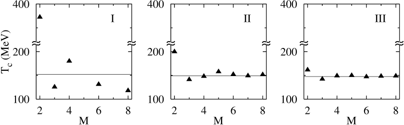
FIG. 3.: Dependence of the critical temperature on the order of expansion for the three cutoffs. The solid lines represent the grid values. Note the cut on the y-axis. See text.

FIG. 4.: Correlation of the pion decay constant at zero temperature and the critical temperature (left) for cutoff (II). Evolution of the pion decay constant with the momentum scale at the critical temperature (middle) and calculation of the critical exponent for cutoff (II), $M=8$. See text.

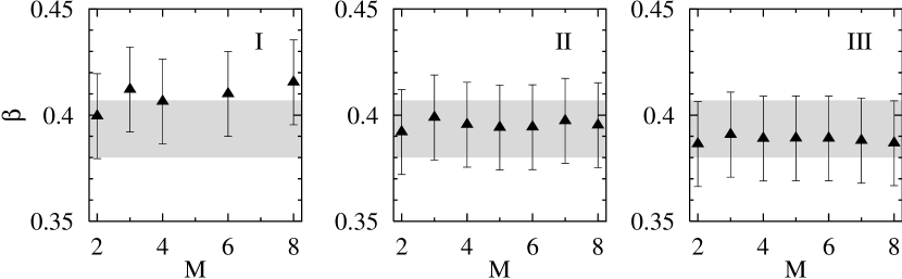
FIG. 5.: The critical exponent $\beta$, for the three cutoffs as the function of the order of the polynomial expansion. The shadowed region represents the $O(4)$ value from different calculations. See text.

TABLE I.: The initial parameters $m$ and $\lambda$ at the scale $k=\Lambda$ for different cutoff functions (I)–(III) and the resulting pion decay constant $f_{\pi}$, at the scale $k\to 0$. The chiral symmetry breaking scale $k_{\chi SB}$, is also given.

cutoff function	$m{[GeV]}$	$\lambda$	$f_{\pi}[MeV]$	$k_{\chi SB}[GeV]$
(I)	$0.4$	$51.5$	$91.85$	$0.87$
(II)	$0.4$	$30.0$	$91.86$	$0.98$
(III)	$0.4$	$16.0$	$91.86$	$1.00$