Power corrections and renormalon resummation for the average thrust

Abstract

Infrared power corrections for the average thrust $\left<T\right>$ in $e^{+}e^{-}$ annihilation are analyzed in the framework of renormalon resummation, motivated by analogy with the skeleton expansion in QED and the BLM approach. Performing the “massive gluon” renormalon integral a renormalization scheme invariant result is obtained. We find that a major part of the discrepancy between the known next-to-leading order (NLO) calculation and experiment can be explained by resummation of higher order perturbative terms. This fact does not preclude the infrared finite coupling interpretation with a substantial $1/Q$ power term. Fitting the regularized perturbative sum plus a $1/Q$ term to experimental data yields $\alpha_{s}^{\hbox{$\overline{\hbox{\tiny MS}}\,$}}({\rm M_{Z}})=0.110\pm 0.006$.

1 Introduction

Power corrections to event shape observables in $e^{+}e^{-}$ annihilation have been an active field of research in the recent years. Event shapes, as opposed to other inclusive observables, do not have an operator product expansion, so there is no established field theoretic framework to analyse them beyond the perturbative level. On the other hand, the experimental data now available cover a wide range of scales and thus could provide an opportunity to test QCD and extract a precise value of $\alpha_{s}$.

The state of the art in perturbative calculations of average event shape variables is ${\cal O}(\alpha_{s}^{2})$, i.e. NLO. It turns out that experimental data are not well described by these perturbative expressions, unless explicit power corrections, that may be associated with hadronization, are introduced. Renormalon phenomenology allows to predict the form of the power terms while their magnitude is determined by experimental fits.

In the work reported here [1] we assume the existence of an Abelian like “dressed skeleton expansion” in QCD and calculate the single dressed gluon contribution using the dispersive approach. This way we perform at once all order resummation of perturbative terms which are related to the running coupling (renormalons) and parametrization of power corrections. We discuss the ambiguity between the perturbative sum and the power corrections and show that the resummation is essential in order to extract the correct value of $\alpha_{s}$ from experimental data.

2 Average thrust in perturbation theory

To demonstrate the method proposed we concentrate on one specific observable, the average thrust, defined by

$$T=\frac{\sum_{i}\left|\vec{p}_{i}\cdot\vec{n}_{T}\right|}{\sum_{i}\left|\vec{p}_{i}\right|},$$ (1)

where $i$ runs over all the particles in the final state, $\vec{p}_{i}$ are the 3-momenta of the particles and $\vec{n}_{T}$ is the thrust axis which is set such that $T$ is maximized. It is useful to define $t\equiv 1-T$ which vanishes in the 2-jet limit.

Being collinear and infrared safe, the average thrust can be calculated in perturbative QCD to yield

$$\left<t\right>_{\hbox{\tiny NLO}}(Q^{2})=\frac{C_{F}}{2}\,\left[t_{0}\,a_{\hbox{$\overline{\hbox{\tiny MS}}\,$}}(Q^{2})\,+\,t_{1}\,a_{\hbox{$\overline{\hbox{\tiny MS}}\,$}}^{2}(Q^{2})\right]$$ (2)

where $a=\alpha_{s}/\pi$, $C_{F}=\frac{4}{3}$ and the coefficients are $t_{0}=1.58$ and $t_{1}=23.7-1.69\,N_{f}$ (see refs. in [1]). Using the world average value of $\alpha_{s}$, $\alpha_{s}^{\hbox{$\overline{\hbox{\tiny MS}}\,$}}({\rm M_{Z}})=0.117$, the NLO perturbative result (2) turns out to be quite far from experimental data. This is shown in fig. 1.

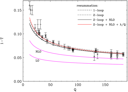
Figure 1: $\left<t\right>$ as a function of $Q=\sqrt{s}$ for $\alpha_{s}^{\hbox{$\overline{\hbox{\tiny MS}}\,$}}(M_{Z})=0.117$. Naive $\overline{\rm MS}$ results (LO, NLO) and resummation results vs experimental data.

From the figure it is clear that the NLO correction is quite significant, so the perturbative series truncated at this order is not very reliable. Furthermore, the renormalization scale dependence is significant. It follows that higher order corrections that are related to the running coupling cannot be ignored.

3 Renormalons and power corrections

In order to take running coupling effects into account it is useful [2] to assume, in analogy with the Abelian theory, that there exists a “dressed skeleton expansion”. Then, the most important corrections which correspond to a single dressed gluon can be written in the form of a renormalon integral

$$D_{0}=\int_{0}^{\infty}\frac{dk^{2}}{k^{2}}\,\phi(k^{2}/Q^{2})\,\bar{a}(k^{2})$$ (3)

where $\bar{a}$ represents a specific “skeleton effective charge”, not yet determined in QCD (in [1] several schemes were used). As opposed to the standard perturbative approch (2), by performing the integral (3) over all scales one avoids completely renormalization scale dependence.

The integral (3) represents a non Borel summable power series. Indeed, it involves integration over the coupling constant in the infrared which is ill-defined in perturbation theory due to Landau singularities. The ambiguous integral (3) can be defined mathematically, e.g. as a principle value of the Borel sum: $D_{0}|_{\hbox{\tiny PV}}$. This, however, does not solve the physical problem of infrared renormalons: information on large distances is required to fix the ambiguity. The perturbative calculation contains some information about the ambiguity: if the leading term in the small momentum expansion of $\phi$ is $\phi(k^{2}/Q^{2})=C_{n}(k^{2}/Q^{2})^{n}$, the leading infrared renormalon is located at $n/\beta_{0}$ in the Borel plane, and a power correction of the form $1/Q^{2n}$ is expected. Having no way to handle the problem on the non-perturbative level, it is natural to attempt a fit of the form $D_{0}|_{\hbox{\tiny PV}}+\lambda/Q^{2n}$.

A stronger assumption [3] is that the “skeleton coupling” can be defined on the non-perturbative level down to the infrared. Then the integral (3) should give at once the perturbative result plus the correct power term. Since the infrared coupling is not known, it is considered as a non-perturbative parameter. Using the cutoff regularization of (3), one fits the data with $D_{0}|_{\mu_{I}}+\lambda_{\mu_{I}}/Q^{2n}$, where

$$D_{0}|_{\mu_{I}}=\int_{\mu_{I}^{2}}^{\infty}\frac{dk^{2}}{k^{2}}\,\phi(k^{2}/Q^{2})\,\bar{a}(k^{2})$$ (4)

is fully under control in perturbation theory and the normalization of the power term

$$\lambda_{\mu_{I}}=C_{n}\int_{0}^{\mu_{I}^{2}}\frac{dk^{2}}{k^{2}}\,k^{2n}\,\bar{a}(k^{2})$$ (5)

is a perturbatively calculable coefficient times a moment of the coupling in the infrared. Since the coupling is assumed to be universal, the magnitude of power corrections can be compared between different observables [3].

The generalization of this approach to Minkowskian observables such as the thrust was discussed in [3, 1]. At the level of a single gluon emission it is based on a “gluon mass” renormalon integral [4]

$$R_{0} \equiv \int_{0}^{\infty}{d\mu^{2}\over\mu^{2}}\ \bar{a}_{\hbox{\tiny eff}}(\mu^{2})\ \dot{{\cal F}}(\mu^{2}/Q^{2})$$ (6)

where the characteristic function ${\cal F}$ is calculated based on the matrix element for the emission of one massive gluon and $\bar{a}_{\hbox{\tiny eff}}$ is related to the time-like discontinuity of the coupling. Regularizations of the perturbative sum (6) with $\bar{a}$ at one or two loops were discussed in [1]. We skip it here for brevity.

4 Fitting experimental data

In order to perform renormalon resummation at the level of a single gluon emission, we calculated the characteristic function for the thrust [1]. Then $R_{0}$ is evaluated taking either the one or two loop coupling. Since $R_{0}$ does not exhaust the full NLO correction of eq. (2), we add an explicit NLO correction, $\delta_{\hbox{\tiny NLO}}=\left(t_{1}-t_{1}^{0}\right)a_{\hbox{$\overline{\hbox{\tiny MS}}\,$}}^{2}$, where $t_{1}$ corresponds to (2) and $t_{1}^{0}$ is the piece included in $R_{0}$. It was shown in [1] that the Abelian part of $t_{1}^{0}$ almost coincides with that of $t_{1}$ in spite of the non-inclusive nature of the thrust. This is crucial for the applicability of the current resummation approach. Finally, we add an explicit power correction $\lambda/Q^{2n}=\lambda/Q$ where the power $n=\frac{1}{2}$ is determined from the small $\mu^{2}$ expansion of ${\cal F}$. Thus, using the PV regularization of $R_{0}$, we fit the data with

$$\left<t\right>=\frac{C_{F}}{2}\left[R_{0}|_{\hbox{\tiny PV}}+\delta_{\hbox{\tiny NLO}}\right]+\frac{\lambda}{Q}.$$ (7)

The resummation as well as the fit results are presented in fig. 1 for the world average value of $\alpha_{s}$. The resummation by itself is quite close to the data. Note also the stability of the result as $\bar{a}$ is promoted from one to two loops. Next, we fit also the value of $\alpha_{s}$. The best fit $\chi^{2}/{\rm point}=1.35$, obtained with $\alpha_{s}^{\hbox{$\overline{\hbox{\tiny MS}}\,$}}(M_{Z})=0.110\pm 0.006$ and $\lambda=0.62\pm 0.11$, is shown in fig. 3.

5 Truncated expansions in $\overline{\rm MS}$

It is interesting to compare the resummation to a truncated expansion in $a_{\hbox{$\overline{\hbox{\tiny MS}}\,$}}$. Expanding $R_{0}$ with $\bar{a}$ at 1-loop we obtain a series of the form $\sum_{i=0}^{\infty}t_{i}^{0}a_{\hbox{$\overline{\hbox{\tiny MS}}\,$}}^{i+1}$. The coefficients $t_{i}^{0}$ can be considered as predictions for the perturbative coefficients $t_{i}$, provided the coupling $\bar{a}$ is close to the correct “skeleton coupling”, and provided that the “leading skeleton” $R_{0}$ is indeed dominant already in the sub-asymptotic regime. The significance of the NNLO and further sub-leading corrections which correspond to the dissociation of the emitted gluon is demonstrated in fig. 2. The figure shows

$$\left<t\right>_{\rm pert} \equiv \left<t\right>_{\hbox{\tiny NLO}}+\frac{C_{F}}{2}\sum_{i=3}^{k}\,t_{i-1}^{0}\,a_{\hbox{$\overline{\hbox{\tiny MS}}\,$}}^{i}(Q^{2})$$ (8)

where $k$ is the order of truncation for $k=2$ through $6$. At these orders the series is still convergent.

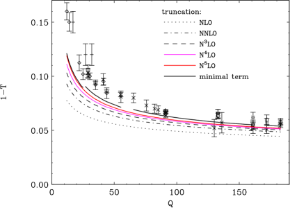
Figure 2: $\left<t\right>_{\rm pert}$ as a function of $Q$ for $\alpha_{s}^{\hbox{$\overline{\hbox{\tiny MS}}\,$}}({\rm M_{Z}})=0.111$. The perturbative series is gradually improved by adding terms from $R_{0}$.

We conclude that a major part of the discrepancy between the NLO result and experiment is due to neglecting this particular class of higher order corrections. Next consider a fit to experimental data based on the truncated expansion of $R_{0}$ (8): $\left<t\right>_{\rm pert}+{\lambda_{\rm pert}}/{Q}$. The fit results are listed in table 1.

Table 1: Fit results based on the truncated expansion in $\overline{\rm MS}$

$$\begin{array}[]{ccc}\hline\cr\,k&\,\alpha_{s}^{\hbox{$\overline{\hbox{\tiny MS}}\,$}}({\rm M_{Z}})&\,\lambda_{\rm pert}\,({\rm GeV})\\ \hline\cr 2&0.128&0.72\\ 3&0.118&0.65\\ 4&0.115&0.58\\ 5&0.114&0.50\\ 6&0.114&0.40\\ \hline\cr{\rm PV}&0.111&0.73\\ \hline\cr\end{array}$$

The quality of the fit is roughly the same in all cases. We see that the resummation is absolutely necessary in order to extract a reliable value of $\alpha_{s}$.

6 Infrared cutoff regularization

Putting an infrared cutoff $\mu_{I}$ on the space-like momentum (4) we separate at once the perturbative and non-perturbative regimes as well as large and small distances. The cutoff regularized sum, $R_{0}|_{\mu_{I}}$ for $\mu_{I}=2\,{\rm GeV}$ is shown in fig. 3 together with the PV regularization.

Figure 3: $\left<t\right>$ as a function of $Q$ for $\alpha_{s}^{\hbox{$\overline{\hbox{\tiny MS}}\,$}}({\rm M_{Z}})=0.110$. Resummation in different regularizations and a fitted curve based on either of them.

For the lower $Q$ values the difference between the two regularizations is large. This means that a large contribution to $R_{0}|_{\hbox{\tiny PV}}$ comes from momentum scales below $2\,{\rm GeV}$, where the coupling is not controlled by perturbation theory. Finally fitting the data

$$\left<t\right>=\frac{C_{F}}{2}\left[R_{0}|_{\mu_{i}}+\delta_{\hbox{\tiny NLO}}\right]+\frac{\lambda_{\mu_{I}}}{Q}$$ (9)

we get the same result as with the PV regularization (7). The only difference is in the required power correction $\lambda_{\mu_{I}}=1.49$. This is general: the two regularizations differ just by (calculable) infrared power corrections – in our case $1/Q$ – and are therefore equivalent once the appropriate power terms are included.

7 Conclusions

The assumption of a “skeleton expansion” implies that resummation of perturbation theory and parametrization of power corrections must be performed together. For the thrust renormalon resummation is significant and closes most of the gap between the standard perturbative result (NLO) and experiment. The resummation is crucial to extract the correct value of $\alpha_{s}$.

The infrared sensitivity of the thrust leads to ambiguity in the resummation, which is settled by fitting a $1/Q$ term. In the infrared cutoff regularization this power term is substantial.

The resummation leads to a renormalization scale invariant result. In the BLM approach it corresponds to a low renormalization point in $\overline{\rm MS}$, $\mu_{\hbox{\tiny BLM}}^{\hbox{$\overline{\hbox{\tiny MS}}\,$}}\simeq 0.0447\,Q$.

E. De Rafael What is the physical meaning, in QCD, of the scale of the $1/Q$ correction? What other processes are sensitive to these corrections?

The first question is basically an open one. Deeper understanding could hopefully be gained once renormalon phenomenology is supported by more rigorous field theoretic methods. In the infrared finite coupling approach the $1/Q$ correction is understood as a moment (5) of a universal infrared finite coupling. This allows comparison between observables – for example the C parameter is sensitive to similar $1/Q$ corrections. In the framework of shape-functions [5], a relation with the energy-momentum tensor was suggested.

References

- [1] E. Gardi and G. Grunberg, [hep-ph/9908458].
- [2] S.J. Brodsky, G.P. Lepage and P.B. Mackenzie, Phys. Rev. D28 (1983) 228.
- [3] Yu.L. Dokshitzer, G. Marchesini and B.R. Webber, Nucl. Phys. B469 (1996) 93.
- [4] M. Beneke and V.M. Braun, Phys. Lett. B348 (1995) 513.
- [5] G.P. Korchemsky and G. Sterman, [hep-ph/9902341].