Estimating $\varepsilon^{\prime}/\varepsilon$ . A user’s manual

Abstract

I review the current theoretical estimates of the CP-violating parameter $\varepsilon^{\prime}/\varepsilon$ , compare them to the experimental result and suggest a few guidelines in using the theoretical results.

1 Notation

The parameter $\varepsilon^{\prime}$ measures direct CP violation and is defined by the difference of the amplitude ratios

$$\varepsilon^{\prime} = \frac{\varepsilon}{\sqrt{2}}\left\{\frac{\langle(\pi\pi)_{I=2}|{\cal L}_{W}|K_{L}\rangle}{\langle(\pi\pi)_{I=0}|{\cal L}_{W}|K_{L}\rangle}\right.$$ (1)

$$\quad\quad\quad\quad-\left.\frac{\langle(\pi\pi)_{I=2}|{\cal L}_{W}|K_{S}\rangle}{\langle(\pi\pi)_{I=0}|{\cal L}_{W}|K_{S}\rangle}\right\}\,,$$

where $K_{L,S}$ are the long- and short-lived neutral kaons, and $\varepsilon$ measures indirect CP violation in the same system.

It is useful to recast eq. (1) in the form

$$\frac{\varepsilon^{\prime}}{\varepsilon}=\frac{G_{F}\omega}{2\left|\epsilon\right|\mathop{\mbox{Re}}{A_{0}}}\>\mbox{Im}\,\lambda_{t}\>\left[\Pi_{0}-\frac{1}{\omega}\>\Pi_{2}\right]\;,$$ (2)

where, referring to the $\Delta S=1$ quark hamiltonian

$${\cal H}_{W}=\sum_{i}\frac{G_{F}}{\sqrt{2}}V_{ud}\,V^{*}_{us}\Bigl{[}z_{i}(\mu)+\tau\ y_{i}(\mu)\Bigr{]}\;Q_{i}(\mu)\,,$$ (3)

we have that

$$\Pi_{0} = \frac{1}{\cos\delta_{0}}\sum_{i}y_{i}\,\mathop{\mbox{Re}}\langle Q_{i}\rangle_{0}\ (1-\Omega_{\eta+\eta^{\prime}})\;,$$ (4)

$$\Pi_{2} = \frac{1}{\cos\delta_{2}}\sum_{i}y_{i}\,\mathop{\mbox{Re}}\langle Q_{i}\rangle_{2}\,,$$ (5)

where the Wilson coefficients $z_{i}$ and $y_{i}$ are known to the next-to-leading order in $\alpha_{s}$ and $\alpha_{e}$ [2]. The four-quark operators $Q_{1\cdots 10}$ are the standard set

$$\begin{array}[]{rcl}Q_{1}&=&\left(\overline{s}_{\alpha}u_{\beta}\right)_{\rm V-A}\left(\overline{u}_{\beta}d_{\alpha}\right)_{\rm V-A}\,,\\[4.30554pt] Q_{2}&=&\left(\overline{s}u\right)_{\rm V-A}\left(\overline{u}d\right)_{\rm V-A}\,,\\[4.30554pt] Q_{3,5}&=&\left(\overline{s}d\right)_{\rm V-A}\sum_{q}\left(\overline{q}q\right)_{\rm V\mp A}\,,\\[4.30554pt] Q_{4,6}&=&\left(\overline{s}_{\alpha}d_{\beta}\right)_{\rm V-A}\sum_{q}(\overline{q}_{\beta}q_{\alpha})_{\rm V\mp A}\,,\\[4.30554pt] Q_{7,9}&=&\frac{3}{2}\left(\overline{s}d\right)_{\rm V-A}\sum_{q}\hat{e}_{q}\left(\overline{q}q\right)_{\rm V\pm A}\,,\\[4.30554pt] Q_{8,10}&=&\frac{3}{2}\left(\overline{s}_{\alpha}d_{\beta}\right)_{\rm V-A}\sum_{q}\hat{e}_{q}(\overline{q}_{\beta}q_{\alpha})_{\rm V\pm A}\,,\end{array}$$ (6)

and the hadronic matrix elements are taken along the isospin direction $I=0$ and 2. Accordingly, $A_{0}$ is the amplitude $A(K^{0}\rightarrow\pi\pi,I=0)$ and $\omega$ is the ratio $\mathop{\mbox{Re}}A_{2}/\mathop{\mbox{Re}}A_{0}$, the smallness of which goes under the name of the $\Delta I=1/2$ rule; it plays an important role in the theoretical prediction of $\varepsilon^{\prime}$ . The parameters $\tau\equiv-V_{td}V_{ts}^{*}/V_{ud}V_{us}^{*}$ and $\mathop{\mbox{Im}}\lambda_{t}\equiv V_{td}\,V^{*}_{ts}$ are combinations of Cabibbo-Kobayashi-Maskawa coefficients. See the review on $\varepsilon^{\prime}/\varepsilon$ in ref. [1] for the definition of the isospin-breaking correction $\Omega_{\eta+\eta^{\prime}}$ and the final-state interaction phases $\delta_{0,2}$ as well as more details on the definitions above.

2 Preliminary remarks

Let us go back to eq. (2), where

$$\frac{G_{F}\omega}{2|\varepsilon|\,\mbox{Re}\,A_{0}}\simeq 10^{3}\>\mbox{GeV}^{-3}\,.$$ (7)

If we were to take

$$\Pi_{0,2}\simeq\frac{\alpha_{s}}{\pi}\,[m_{K}]^{3}\simeq 10^{-2}\>\mbox{GeV}^{-3}\,,$$ (8)

that is, estimating the hadronic matrix elements by simple dimensional analysis ($\alpha_{s}/\pi$ takes into account the size of QCD induced Wilson coefficients), and

$$\mbox{Im}\,\lambda_{t}\simeq 10^{-4}\,,$$ (9)

which is certainly reasonable, we would obtain

$$\varepsilon^{\prime}/\varepsilon\simeq 10^{-3}\,,$$ (10)

a back-of-the-envelope estimate which is remarkably close to the experimental result. What is then the problem?

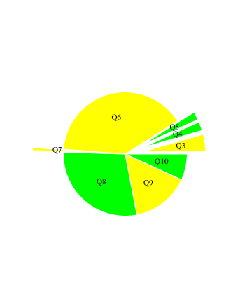
Consider the contribution of the various operators in the (very simple minded) vacuum saturation approximation for the hadronic matrix elements. Figure 1 visualizes this computation in a pie chart that graphically shows how the contributions come with different signs and that cancellations among them can be sizable. Dimensional analysis cannot be assumed to be reliable in the presence of such large cancellations and therefore the result (10) cannot be trusted.

Figure 1: The pie chart: In yellow/light-gray (green/dark-gray) positive (negative) contributions to $\varepsilon^{\prime}/\varepsilon$ of the effective operators $Q_{1\cdot 10}$. Hadronic matrix elements in the vacuum saturation approximation.

The actual cancellation depends on the size of the hadronic matrix elements $\langle Q_{i}\rangle_{0,2}$, the estimate of which requires some control on the non-perturbative part of QCD. This is by far the main source of uncertainty in any theoretical estimate of $\varepsilon^{\prime}/\varepsilon$ . In addition, also the determination of the overall factor $\mathop{\mbox{Im}}\lambda_{t}$ depends on the non-perturbative amplitude for the transition of $K^{0}-\bar{K}^{0}$, thus making the final uncertainty even larger. 

It is on the basis of such a cancellation that, in the early 90s, the idea that $\varepsilon^{\prime}/\varepsilon$ could be very small—of the order of $O(10^{-4})$ if not altogether vanishing (thus mimicking the super-weak scenario)—took hold of the theoretical community.  At the same time, the discrepancy between the two experimental results and in particular the smallness of the FNAL result played a role in favor of a small $\varepsilon^{\prime}/\varepsilon$ .

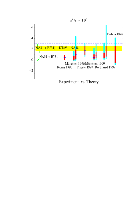
It is only this year (1999) that the (preliminary) results from the new-generation experiments have finally settled the question of the size of $\varepsilon^{\prime}/\varepsilon$and converged on the value

$$\varepsilon^{\prime}/\varepsilon=(2.1\pm 0.46)\times 10^{-3}$$ (11)

which is obtained by averaging over the preliminary results for the 1998-99 experiments (KTeV [3] and NA48 [4]) as well as those in 1992-93 (NA31 [5] and E731 [6]). The result in eq. (11) rules out the super-weak scenario and makes possible a detailed comparison with and among the theoretical analyses.

3 Experiment vs. theoretical estimates

Given the fact that the gluon and electroweak penguin operator tend to cancel each other contribution to $\varepsilon^{\prime}/\varepsilon$ , the question is whether this cancellation is as effective as reducing by one order of magnitude the back-of-the-envelope estimate of the previous section or not.

Before the publication of this year experimental results, there were three estimates of $\varepsilon^{\prime}/\varepsilon$ . Two of them (Münich and Rome) for which the cancellation took place and one (Trieste) for which it did not.

The situation has not really changed this year, except for those new estimates that have come out, partially confirming the Trieste prediction of a large $\varepsilon^{\prime}/\varepsilon$ .

To compare different approaches, it is useful to introduce the parameters

$$B_{i}(\mu)^{(0,2)}=\frac{\langle Q_{i}\rangle_{0,2}}{\langle Q_{i}\rangle_{0,2}^{VSA}}$$ (12)

which give the correction in the approach with the respect to the result in the vacuum saturation approximation (VSA). Let me stress that there is nothing magical about the VSA: it is just a convenient (but arbitrary) normalization point. Accordingly, there is no reason whatsoever to prefer values of $B_{i}=1$ and most the cases in which the parameters have been computed they have greatly deviated from 1—a case in point is the parameter $B_{1}^{(0)}$, which can be determined from the CP conserving amplitude $A_{0}$ and is ten times bigger than its VSA value because of the $\Delta I=1/2$ rule.

	(ph)	(lattice)	($\chi$QM)
$B_{i}$	$\mu=1.3$ GeV	$\mu=2.0$ GeV	$\mu=0.8$ GeV
$B_{1}^{(0)}$	13 (†)	-	9.5
$B_{2}^{(0)}$	$6.1\pm 1.0$ (†)	-	2.9
$B_{1}^{(2)}=B_{2}^{(2)}$	0.48 (†)	-	0.41
$B_{3}$	1 (*)	1 (*)	$-2.3$
$B_{4}$	5.2 (*)	$1\div 6$ (*)	1.9
$B_{5}\simeq B_{6}$	$1.0\pm 0.3$ $(*)$	$1.0\pm 0.2$ $(*)$	$1.6\pm 0.3$
$B_{7}^{(0)}\simeq B_{8}^{(0)}$	1 (*)	1 (*)	$2.5\pm 0.1$
$B_{9}^{(0)}$	7.0 (*†)	1 (*)	3.6
$B_{10}^{(0)}$	7.5 (*†)	1 (*)	4.4
$B_{7}^{(2)}$	1 (*)	$0.6\pm 0.1$	$0.92\pm 0.02$
$B_{8}^{(2)}$	$0.8\pm 0.2$ $(*)$	$0.8\pm 0.15$	$0.92\pm 0.02$
$B_{9}^{(2)}$	0.48	$0.62\pm 0.10$	0.41
$B_{10}^{(2)}$	0.48	1 (*)	0.41
$B_{K}$	$0.80\pm 0.15$	$0.75\pm 0.15$	$1.1\pm 0.2$

Table 1: The $B_{i}$ factors in three approaches. (${\dagger}$) stands for an input value and (*) for an “educated guess”.

Table 1 collects the $B_{i}$ parameter for three approaches. Notice that larger values of $B_{K}$ give smaller values for $\mathop{\mbox{Im}}\lambda_{t}$ and accordingly for $\varepsilon^{\prime}/\varepsilon$ . In discussing the various approaches, it is important to bear in mind that a $B_{i}$ parameter, being normalized on the VSA, could depend on a quantity, like $m_{s}$, even when the estimate itself does not.

Let consider the two most relevant operators $B_{6}$ and $B_{8}$. There is overall agreement among the various approaches on $B_{8}$. On the other hand, for the crucial parameter $B_{6}$ the Münich and Roma group must relay on an “educated guess” and only the Trieste group provides a computed value. For this reason, I think that is fair to say that both the Münich and Roma  estimate suffer of a systematic bias in so far as the crucial parameter $B_{6}$ is not estimated but simply varied around the large $1/N_{c}$ (vacuum saturation) result. In a computation that essentially consists in the difference between two contributions, the fact that one of the two is simply assumed to vary around a completely arbitrary central value casts some doubts about any statement about unlikely corners of parameter space for which the current experimental result can be reproduced by the theory.

4 Extended caption to Fig. 2

The simplest way of summarizing the present status of theoretical estimates of $\varepsilon^{\prime}/\varepsilon$ consists in explaining Fig. 2. Let us group the various estimated according on whether they were published before or after the last run of experiments (early 1999), in other words, between those published when the value of $\varepsilon^{\prime}/\varepsilon$ was still uncertain and those after it has been determined to be $\approx 2\times 10^{-3}$. The various approaches substantially agree on the short-distance analysis and inputs and therefore I will only discuss here the long-distance part. 

• Pre-dictions:

  • Roma 1996 [8] It is based on the lattice simulation of non-perturbative QCD. The hadronic matrix elements are included using the lattice simulation for those known and “educated guesses” for those which are not known. Only the Gaussian treatment of the uncertainties (red/dark-gray bar) is given.

  • Münich 1996 [9] It is based on a mixture of phenomenological and $1/N_{c}$ approach in which as many as possible of the matrix elements are determined by means of known CP conserving amplitudes and those remaining by leading $1/N_{c}$ estimates. Both the flat scanning (light-blue/light-gray) and the Gaussian treatment (red/dark-gray) of the uncertainties is given. The two values correspond to two different choices for the strange quark mass.

  • Trieste 1997 [10] It is based on the chiral quark model. All matrix elements are parameterized in terms of three parameters: the quark and gluon condensates and the constituent quark mass. The values of these parameters are determined by fitting the $\Delta I=1/2$ rule. Chiral perturbation corrections are included to the complete $O(p^{4})$. Both the flat scanning (light-blue/light-gray) and the Gaussian treatment (red/dark-gray) of the uncertainties is given. 

• Post-dictions

  • Münich 1999 [11] It is an updated analysis similar to that of 1996. The two ranges are now those obtained by using the Wilson coefficients in the HV and NDR regularization prescription. Again, both the flat scanning (light-blue/light-gray) and the Gaussian treatment (red/dark-gray) of the uncertainties is given.

  • Dortmund 1999 [12] It is based on the $1/N_{c}$ estimate of the hadronic matrix elements, regularized by means of an explicit cutoff. Chiral perturbation corrections are included (partially) up to $O(p^{4})$. Two estimates are given according to whether the input parameters are kept fixed (red/dark-gray) or varied (light-blue/light-gray). The second range given corresponds to the inclusion of important $O(p^{4})$ corrections. No central values are given.

  • Dubna 1999 [13] It is based on chiral perturbation theory up to $O(p^{6})$. I cannot say much about it because it came out just at the time of this conference. I have included their full range according to the tables reported in the reference above (flat scanning in light-blue/light-gray, the Gaussian treatment in red/dark-gray).

Figure 2: Experiment vs. theoretical estimates. See text for full caption.

5 Strengths and weaknesses of the various approaches

Since there is no estimate which is safe from criticism, I would like to try to summarize the strengths and weaknesses of the various approaches and leave it to the reader to decide by himself.

• Roma

  • Good: The lattice approach is well-grounded in first-principles.

  • Bad: Half of the computation is missing: there is no determination of $B_{6}$, the value of which must be guessed.

• Münich

  • Good: Clever use of CP conserving amplitudes. Determination of many $B_{i}$ in a model-independent manner.

  • Bad: The important parameters $B_{8}$ and $B_{6}$ cannot be determined and must be varied around their leading $1/N_{c}$ values.

• Trieste

  • Good: All operators ($Q_{6}$ included) are determined in a consistent manner; the full $O(p^{4})$ chiral perturbation is included.

  • Bad: Phenomenological model which is not derivable from first principle. There is a uncertainty in the matching procedure which is difficult to estimate.

• Dortmund

  • Good: State-of-the-art $1/N_{c}$ estimate of all matrix elements.

  • Bad: Potentially important $O(p^{4})$ not included yet in the analysis. Unstable matching and therefore very large uncertainties.

6 The lesson of the chiral quark model result

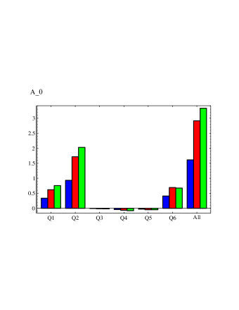
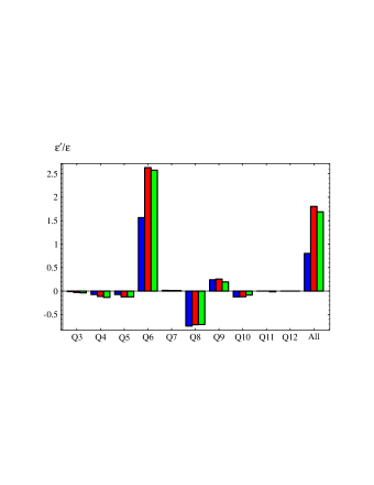
The crucial enhancement of the parameter $B_{6}$ in the chiral quark model originates in the fit of the $\Delta I=1/2$ rule that is at the basis of this model. We could say that it is a revival of the old idea [14] of having the same gluon penguin operator explaining the $\Delta I=1/2$ also give a large $\varepsilon^{\prime}/\varepsilon$ (see Fig. 4). This mechanism works only at a scale around 1 GeV and is not as complete as in the original idea (in the chiral quark model the penguin contribution to the $A_{0}$ amplitude turns out to be about 20%, see Fig. 3). Clearly for approaches based on scales higher than $m_{c}$ a different mechanism must be at work to mimic the same effect (given the scale invariance of the physical amplitudes).

Figure 3: The amplitude $A_{0}$ in the chiral quark model. The contribution of the gluon penguin operator to order $O(p^{4})$ (green/light-gray histogram) is about 20% of the total.

Figure 4: Anatomy of $\varepsilon^{\prime}/\varepsilon$ in the chiral quark model. The ratio is dominated by the gluon penguin operator $Q_{6}$ but only after all correction order $O(p^{4})$ are included (the green/light-gray histogram).

7 Conclusion

As Fig. 2 makes it clear, there is no disagreement between the experimental result and the prediction of the standard model once all uncertainties are properly taken into account. Of the five available estimates today (August 1999), three  overlap with the experimental range and one of them (Trieste) even predicted it two years in advance of the experiments.  Only the Rome and Münich estimates are somewhat below the current experimental range but they suffer of a systematic uncertainty, as discussed in the previous section.

If we abstract from the details and the central values of the various estimates, it is comforting that in such a complicated computation, different approaches give results that are rather consistent among themselves (namely, values of $\varepsilon^{\prime}/\varepsilon$ positive and of the order of $O(10^{-3})$) and in overall agreement with the experiment. This, I think, is the most important message.

A final word on possible future improvements.

The place where to look for a reduction of the present theoretical uncertainties is $\mathop{\mbox{Im}}\lambda_{t}$. Ideally, this coefficient could be determined in a manner that is free of non-perturbative uncertainties in the process $K_{L}\to\pi^{0}\bar{\nu}\nu$. Such a determination could easily reduce the uncertainty in $\varepsilon^{\prime}/\varepsilon$ by 20-30%.

On the front of hadronic matrix elements, work is in progress on various phenomenological approaches as well as on lattice simulations.

Question (M. Neubert, SLAC): What is the basis for the “educated guesses” leading to values of $B_{6,8}$ close to one, given that all the other B-parameters known from data show very large deviations form the vacuum saturation approximation?

Answer: My very same objection. Anyway, some come from leading $1/N_{c}$ estimates, some are just guesses.

Question (L. Giusti, Boston Univ.): Which $B_{K}$ do you use to extract $\mathop{\mbox{Im}}\lambda_{t}$ in the chiral quark model?

Answer: That determined in the chiral quark model, see Table 1. As a matter of fact, it is because in this model $B_{K}$ comes out larger than in other estimates that $\varepsilon^{\prime}/\varepsilon$ is not even larger.

References

- [1] S. Bertolini, J. Eeg and M. Fabbrichesi, hep-ph/9802405, to appear in Reviews of Modern Physics, January 2000.
-
[2]
A. J. Buras et al, Nucl. Phys. B370 (1992) 69 and
Nucl. Phys. B400 (1993) 37;
A. J. Buras, M. Jamin and M.E. Lautenbacher, Nucl. Phys. B400 (1993) 75 and Nucl. Phys. B408 (1993) 209;
M. Ciuchini, E. Franco, G. Martinelli and L. Reina, Nucl. Phys. B415 (1994) 403. - [3] A. Alavi-Harati et al., Phys. Rev. Lett. 83 (1999) 22.
- [4] P. Debu, seminar at CERN, June 18, 1999 (http://www.cern.ch/NA48).
- [5] G. D. Barr et al., Phys. Lett. B317 (1993) 233.
- [6] L. K. Gibbons et al., Phys. Rev. D55 (1997) 6625.
[7]
R. Gupta, hep-ph/9801412;
G. Martinelli,hep-lat/9810013;
D. Pekurovsky and G. Kilcup, hep-lat/9812019. - [8] M. Ciuchini, Nucl. Phys. B Proc. Suppl. 59 (1997) 149.
- [9] A. J. Buras, M. Jamin and M. E. Leutenbacher, Phys. Lett. B389 (1996) 749.
- [10] S. Bertolini et al., Nucl. Phys. B514 (1998) 93.
- [11] S. Bosch et al., hep-ph/9904408
- [12] T. Hambye et al., hep-ph/9906434.
- [13] A. A. Bel’kov et al. , hep-ph/9907335.
[14]
A. I. Vainshtein et al., JEPT 45 (1977) 670;
F. J. Gilman and M. B. Wise, Phys. Lett. B83 (1979)83;
B. Guberina and R. D. Peccei, Nucl. Phys. B163 (1980) 289.