Multilepton production via top flavour-changing neutral couplings at the CERN LHC

Abstract

$Zt$ and $\gamma t$ production with $Z\to l^{+}l^{-}$ and $t\to Wb\to l\nu b$ provides the best determination of top flavour-changing neutral couplings at the LHC. The bounds on $tc$ couplings eventually derived from these processes are similar to those expected from top decays, while the limits on $tu$ couplings are better by a factor of two. The other significant $Z$ and $W$ decay modes are also investigated.

PACS: 12.15.Mm, 12.60.-i, 14.65.Ha, 14.70.-e

1 Introduction

Future colliders will explore higher energies looking for new physics. Even if there is not a new production threshold the top quark will probe the physics beyond the Standard Model (SM). Large $e^{+}e^{-}$ and hadron colliders, in particular the CERN Large Hadron Collider (LHC), will be top factories allowing to measure the top couplings with high precision. Both types of machines are complementary for if the LHC will produce many more tops, $e^{+}e^{-}$ linear colliders will face smaller backgrounds. Nevertheless the most realistic estimates indicate that the precision which can be reached for flavour-changing neutral (FCN) couplings can be up to a factor of three better at the LHC with a luminosity of 100 fb^-1 [1, 2] than at a 500 GeV $e^{+}e^{-}$ linear collider with a luminosity of 100 fb^-1 (LC) [3]. The top couplings which can signal to new physics can be diagonal [4] or off-diagonal. We will concentrate on the latter. FCN couplings are very suppressed within the SM but can be large in simple extensions [5]. Hence they are a good place to look for departures from the SM. However present data only allow for FCN couplings large enough to be observed at future colliders for the top quark. In this paper we investigate the sensitivity of the LHC to top FCN gauge couplings. This has already been studied for top decays [1, 2]. We look at $Vt$ production, $V=Z,\gamma$, induced by anomalous top couplings [6, 7], which, as we shall show, provide better limits.

In order to describe FCN couplings between the top, a light quark $q=u,c$ and a $Z$ boson, a photon $A$ or a gluon $G^{a}$ we use the Lagrangian [8]

$$-{\mathcal{L}} = \frac{g_{W}}{2c_{W}}\bar{t}\gamma_{\mu}(X_{tq}^{L}P_{L}+X_{tq}^{R}P_{R})qZ^{\mu}+\frac{g_{W}}{2c_{W}}\bar{t}(\kappa_{tq}^{(1)}-i\kappa_{tq}^{(2)}\gamma_{5})\frac{i\sigma_{\mu\nu}q^{\nu}}{m_{t}}qZ^{\mu}$$ (1)

$$+e\bar{t}(\lambda_{tq}^{(1)}-i\lambda_{tq}^{(2)}\gamma_{5})\frac{i\sigma_{\mu\nu}q^{\nu}}{m_{t}}qA^{\mu}+g_{s}\bar{t}(\zeta_{tq}^{(1)}-i\zeta_{tq}^{(2)}\gamma_{5})\frac{i\sigma_{\mu\nu}q^{\nu}}{m_{t}}T^{a}qG^{a\mu}+{\mathrm{h}.c.}\,,$$

where $P_{R,L}=(1\pm\gamma_{5})/2$ and $T^{a}$ are the Gell-Mann matrices satisfying ${\mathrm{T}r}\,(T^{a}T^{b})=\delta^{ab}/2$. The couplings are constants corresponding to the first terms in the expansion in momenta. This effective Lagrangian contains $\gamma_{\mu}$ terms of dimension 4 and $\sigma_{\mu\nu}$ terms of dimension 5. The $\sigma_{\mu\nu}$ terms are the only ones allowed by the unbroken gauge symmetry, ${\mathrm{S}U(3)}_{c}\times{\mathrm{U}(1)}_{Q}$. Due to their extra momentum factor they grow with the energy and make large colliders the best place to measure them. They are absent at tree-level in renormalizable theories like the SM, where they are also suppressed by the GIM mechanism [9]. However the effective couplings involving the top quark can be large in models with new physics near the electroweak scale. In effective theories with only the SM light degrees of freedom the $\gamma_{\mu}$ terms above also result from dimension six operators after electroweak symmetry breaking. However, if the scales involved are similar, as happens with the top quark mass and the electroweak scale, the $\gamma_{\mu}$ terms can be also large [10]. This is the case in simple SM extensions with vector-like quarks near the electroweak scale [11]. Although rare processes strongly constrain FCN couplings between light quarks [12], the top can have relatively large couplings to the quarks $u$ or $c$, but not to both simultaneously [5]. Thus the third family seems the best place to look for SM departures and Eq. (1) is the lowest order contribution to trilinear top FCN gauge couplings of any possible extension. It is then important to measure them at the LHC [13].

The vertices in Eq. (1) are constrained by the nonobservation of the top decays $t\to qV$ [14] and $t\to qg$ [15] at Tevatron, implying the present direct limits

$$X_{tq} \equiv \sqrt{|X_{tq}^{L}|^{2}+|X_{tq}^{R}|^{2}}\leq 0.84\,,$$

$$\kappa_{tq} \equiv \sqrt{|\kappa_{tq}^{(1)}|^{2}+|\kappa_{tq}^{(2)}|^{2}}\leq 0.78\,,$$

$$\lambda_{tq} \equiv \sqrt{|\lambda_{tq}^{(1)}|^{2}+|\lambda_{tq}^{(2)}|^{2}}\leq 0.33\,,$$

$$\zeta_{tq} \equiv \sqrt{|\zeta_{tq}^{(1)}|^{2}+|\zeta_{tq}^{(2)}|^{2}}\leq 0.15$$ (2)

at 95% C. L. (Unless otherwise stated, all bounds in this paper have this confidence level.) The sensitivity of the LHC and LC for some of these couplings has been studied for different processes in a series of papers. At the LHC with an integrated luminosity of 100 fb^-1 the expected limits from top decays are $X_{tq}\leq 0.017$ [1], $\lambda_{tq}\leq 0.0035$ [2]. The LC will probe the electroweak couplings in the process $e^{+}e^{-}\to t\bar{c}$, obtaining eventually $X_{tq}\leq 0.051$, $\kappa_{tq}\leq 0.015$, $\lambda_{tq}\leq 0.011$ [3]. The best limits on the $gtq$ vertices are expected from single top production at LHC [16], $\zeta_{tu}\leq 0.0004$, $\zeta_{tc}\leq 0.0009$. In the following we show that the process $gq\to Vt$ gives competitive bounds on the $Vtc$ couplings, $X_{tc}\leq 0.023$, $\kappa_{tc}\leq 0.016$, $\lambda_{tc}\leq 0.0065$, and the best limits on the $Vtu$ vertices, $X_{tu}\leq 0.011$, $\kappa_{tu}\leq 0.0063$, $\lambda_{tu}\leq 0.0021$. This process can take place through the s- and t-channel diagrams in Fig. 1 via $Vtq$ couplings, or via $gtq$ couplings through the diagrams in Fig. 2. However, in the second case the best limits on the strong anomalous couplings $\zeta_{tu}\leq 0.0018$, $\zeta_{tc}\leq 0.0037$ are less stringent than those derived from $tj$ production.

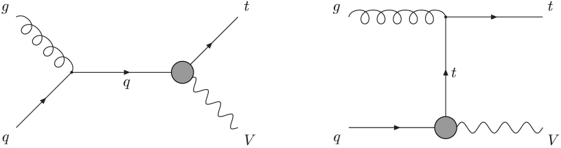
Figure 1: Feynman diagrams for $gq\to Vt$ via $Vtq$ FCN couplings with $V=Z,\gamma$. The $Z$ boson and the top quark are off-shell and have the SM decays.

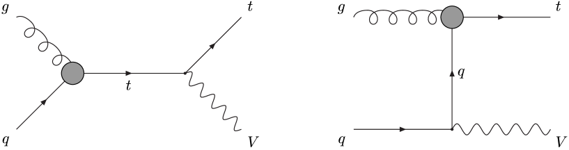
Figure 2: Feynman diagrams for $gq\to Vt$ via $gtq$ FCN couplings with $V=Z,\gamma$. The $Z$ boson and the top quark are off-shell and have the SM decays.

It must be noticed that all upper bounds we shall derive will be obtained following the Feldman-Cousins construction [17] to obtain 95% C. L. intervals, assuming that the number of observed events $n$ equals the expected background $n_{b}$. For the numerical evaluation of the confidence intervals we use the PCI package [18]. The intervals obtained with the Feldman-Cousins construction are similar to standard 95% C. L. upper limits on a Poisson variable with known background [19] but they give less restrictive bounds (see Table 1). Another possibility is to use the 95% C. L. ($1.96\,\sigma$) discovery significance $n_{s}/\sqrt{n_{b}}\geq 1.96$, with $n_{s}$ the expected number of signal events (see for instance Ref. [20]). The limits obtained are similar to standard 95% upper limits when the Poisson distribution can be approximated by a Gaussian ($n_{b}\geq 5$). The quoted limits in Refs. [1, 2, 3, 15, 16] have been obtained using the statistical significance $n_{s}/\sqrt{n_{s}+n_{b}}\geq 3$. This is a conservative estimate with a 99% C. L. and weakens the bounds on the anomalous couplings given here by a factor $\sim\sqrt{2}$ (see Table 1). This is part of the improvement found.

$n_{b}$	$n_{s}$ (Ref. [17])	$n_{s}$ (Ref. [19])	$n_{s}$ (Ref. [20])	$n_{s}$ (Refs. [1, 2, 3, 15, 16])
0	3.09	3.00	0	3.84
5	6.26	5.51	4.38	6.71
10	7.82	6.97	6.20	8.41
15	9.31	8.09	7.59	9.75

Table 1: 95% C. L. upper bounds on signal events $n_{s}$ for samples of $n_{b}$ backgound events obtained using four different prescriptions.

The sensitivity to top FCN couplings varies with the $Z$ and $W$ decay modes. These are collected in Table 2, together with their branching fractions and main backgrounds. We neglect nonstandard top decays since they are a small fraction to start with. Moreover, this approximation becomes better when smaller are the upper limits on anomalous decays, which is the practical case we are interested in. In the leptonic modes we only consider decays to electrons and muons, but a good $\tau$ tagging efficiency increases the leptonic branching ratios in Table 2 and improves their statistical significance. The relevance of the different decay channels results from the balance between the size of the signals, the corresponding backgrounds and their statistical significance, and varies substantially from the Fermilab Tevatron to the LHC. For instance, at Tevatron Run II with a luminosity of 2 fb^-1 the $\nu\bar{\nu}jjb$ decay mode is the most interesting one due to its branching ratio, with 235 signal and 22 background events after kinematical cuts for $X_{tu}=0.84$ [6]. At this collider, the $l^{+}l^{-}l\nu b$ channel has a much larger signal to background ratio (28 signal and 0.07 background events before kinematical cuts for $X_{tu}=0.84$) but still its statistical significance is lower and the bound obtained from the former decay mode is more restrictive. However, this behaviour is reversed at the LHC, where the increase in energy and luminosity makes the $l^{+}l^{-}l\nu b$ channel the most sensitive one.

Other decay modes also provide stringent limits. The $l^{+}l^{-}jjb$ channel gives competitive but worse results than $l^{+}l^{-}l\nu b$ at the LHC. The modes with hadronic $Z$ decay, in particular $jjl\nu b$, which gives significant bounds at Tevatron, have huge backgrounds at higher energies and luminosities: the $Wt$ background becomes more important due to the larger $b$ content of the proton at LHC energies, and $t\bar{t}$, with $t(\bar{t})\to jjb$, $\bar{t}(t)\to l\nu b$ and one jet undetected, also grows rapidly with the energy. Thus the $jjl\nu b$ channel is not interesting any more. The situation improves considering only $Z\to b\bar{b}$ and requiring three $b$ tags, but the results are worse than for the channels with $Z\to l^{+}l^{-}$. The $\nu\bar{\nu}jjb$ mode also has as backgrounds $Wt$ and $t\bar{t}$ but we will discuss this signal for illustration, since this mode is the best one at Tevatron. The remaining decay channels $\nu\bar{\nu}l\nu b$, $jjjjb$ and $b\bar{b}jjb$ have too large backgrounds and will not be treated here. The $\gamma l\nu b$ decay mode is the most interesting one in $\gamma t$ production, due to its small $\gamma Wj$ background. $\gamma jjb$ gives also significant but less restrictive limits.

It is worth to note that $b$ tagging plays an essential rôle in enhancing single top signals. The approximately conserved $b$-Parity in the SM [22] allows in practice to get rid of large backgrounds with an even number of $b$ quarks in the final state.

	$W\to l\nu$			$W\to jj$
	Final state		Backgrounds	Final state		Backgrounds
$Z\to l^{+}l^{-}$	$l^{+}l^{-}l\nu b$	$1.5\%$	$ZWj$	$l^{+}l^{-}jjb$	$4.6\%$	$Zjjj$, $ZWj$
$Z\to\nu\bar{\nu}$	$\nu\bar{\nu}l\nu b$	$4.3\%$	$Wj$	$\nu\bar{\nu}jjb$	$13.6\%$	$t\bar{t}$, $Wt$, $Zjjj$
$Z\to b\bar{b}$	$b\bar{b}l\nu b$	$3.3\%$	$t\bar{t}$, $Wt$, $ZWj$, $Wb\bar{b}j$	$b\bar{b}jjb$	$10.2\%$	$b\bar{b}jjj$
$Z\to jj$	$jjl\nu b$	$15.2\%$	$t\bar{t}$, $Wt$, $Wjjj$	$jjjjb$	$47.4\%$	$jjjjj$
$\gamma$ (stable)	$\gamma l\nu b$	$21.8\%$	$\gamma Wj$	$\gamma jjb$	$67.8\%$	$\gamma jjj$, $\gamma Wj$

Table 2: Branching ratios and main backgrounds for the different $Z$ and $W$ decay channels. $j$ and $jj$ include $b$ and $b\bar{b}$ when possible (we neglect the small Cabibbo-Kobayashi-Maskawa mixing angles $V_{ub},V_{cb}\sim 0$ [21]).

This paper is organized as follows. In Section 2 we discuss how the different signals and backgrounds are generated. In Sections 3 and 4 we analyze $Zt$ and $\gamma t$ signals. We summarize in Section 5.

2 Signal and background simulation

In general $Zt$ production yields five fermion final states with at least one $b$ quark $f\!f\!f\!fb$. We evaluate these signals with the exact matrix element for the s- and t-channel diagrams $gq\to Zt\to ZWb\to f\!f\!f\!fb$ (see Figs. 1 and 2). The SM diagrams $gq\to ZWb$ are much smaller in the phase space region of interest and suppressed by small mixing angles, so we neglect them in the signal evaluation. We also ignore interferences from identical fermion interchange in the final state. All fermions are assumed massless except the top quark, and we assume only one type of coupling to be nonzero at a time. We evaluate $\gamma t$ production in a similar way, with the s- and t-channel diagrams $gq\to\gamma t\to\gamma f\!fb$. $t$ and $\bar{t}$ production are summed up in all cases.

The $VWj$ backgrounds are evaluated considering $gq_{u}\to VWq_{d}$, $gq_{d}\to VWq_{u}$ and $q_{u}\bar{q}_{d}\to VWg$ (with $q_{u}=u,c$ and $q_{d}=d,s,b$) plus the charge conjugate processes. We calculate the matrix elements for $gq_{u}\to VWq_{d}$, including the eight SM diagrams and decaying the $Z$ and $W$ afterwards. The matrix elements for the two other processes are obtained by crossing symmetry. Our results are consistent with those given in Ref. [23].

In order to calculate the $Zjjj$, $Zb\bar{b}j$, $Wjjj$ and $Wb\bar{b}j$ backgrounds we use VECBOS [24] modified to include the energy smearing and trigger and kinematical cuts. We also include routines to generate the kinematical distributions. To generate the $\gamma jjj$ background we have further modified VECBOS to produce photons instead of $Z$ bosons. This is done by introducing a ‘photon’ with a small mass $m_{\gamma}=0.1$ GeV and substituting the $Z$ couplings by the photon couplings everywhere. The total width of such ‘photon’ is calculated to be $\Gamma_{\gamma}=1.73\cdot 10^{-3}$ GeV, with an $e^{+}e^{-}$ branching ratio equal to 0.15. We have checked that the results are the same for a heavier ‘photon’ with $m_{\gamma}=1$ GeV and $\Gamma_{\gamma}=1.73\cdot 10^{-2}$ GeV.

We have also to evaluate $Wt$ production, which is similar to the signal $Zt$, but proceeds through the SM process $gb\to Wt\to WWb\to f\!f\!f\!fb$, and is calculated analogously. $t\bar{t}$ production with some particles missed by the detector must be also considered [25]. Finally, $Wj$, $jjjjj$ and $b\bar{b}jjj$ production is so large that makes unnecessary a detailed discussion of the corresponding signals and of the backgrounds themselves. Other possible small backgrounds are neglected [7, 20].

We include throughout the paper a $K$ factor equal to 1.1 for all processes [26] except for $t\bar{t}$ production for which we assume $K=2.0$ [27]. We use MRST structure functions set A [28] with $Q^{2}=\hat{s}$. The cross sections have some dependence on the structure functions chosen but not the trend of our results.

After generating signals and backgrounds we imitate the experimental conditions with a Gaussian smearing of the lepton ($l$), photon ($\gamma$) and jet ($j$) energies [29],

$$\frac{\Delta E^{l,\gamma}}{E^{l,\gamma}}=\frac{10\%}{\sqrt{E^{l,\gamma}}}\oplus 0.3\%\,,~{}~{}~{}~{}\frac{\Delta E^{j}}{E^{j}}=\frac{50\%}{\sqrt{E^{j}}}\oplus 3\%\,,$$ (3)

where the energies are in GeV and the two terms are added in quadrature. For simplicity we assume that the energy smearing for muons is the same as for electrons. We then apply detector cuts on transverse momenta $p_{T}$, pseudorapidities $\eta$ and distances in $(\eta,\phi)$ space $\Delta R$:

$$p_{T}^{l}\geq 15{\mathrm{~{}}GeV}~{},~{}~{}p_{T}^{j}\geq 20{\mathrm{~{}}GeV}~{},~{}~{}p_{T}^{\gamma}\geq 40{\mathrm{~{}}GeV}$$

$$|\eta^{l,j,\gamma}|\leq 2.5~{},~{}~{}\Delta R_{jj,lj,\gamma l,\gamma j}\geq 0.4\,.$$ (4)

For the $Wt$ and $t\bar{t}$ backgrounds, we estimate in how many events we miss the charged lepton and the $b$ or any other jet demanding that their momenta and pseudorapidities satisfy $p_{T}^{l}<15$ GeV, $p_{T}^{j}<20$ GeV or $|\eta^{l,j}|>3$.

For the events to be triggered, we require both the signal and background to fulfil at least one of the trigger conditions [30]. For the first LHC Run with a luminosity of 10 fb^-1 (L),

• one jet with $p_{T}\geq 180$ GeV,

• three jets with $p_{T}\geq 75$ GeV,

• one charged lepton with $p_{T}\geq 20$ GeV,

• two charged leptons with $p_{T}\geq 15$ GeV,

• one photon with $p_{T}\geq 40$ GeV,

• missing energy $E_{T}\!\!\!\!\!\!\!\!\!\not\,\,\,\,\,\,\,\geq 50$ GeV and one jet with $p_{T}\geq 50$ GeV,

and for the second Run with 100 fb^-1 (H),

• one jet with $p_{T}\geq 290$ GeV,

• three jets with $p_{T}\geq 130$ GeV,

• one charged lepton with $p_{T}\geq 30$ GeV,

• two charged leptons with $p_{T}\geq 20$ GeV,

• one photon with $p_{T}\geq 60$ GeV,

• missing energy $E_{T}\!\!\!\!\!\!\!\!\!\not\,\,\,\,\,\,\,\geq 100$ GeV and one jet with $p_{T}\geq 100$ GeV.

Finally, we require a tagged $b$ jet in the final state taking advantage of a good $b$ tagging efficiency $\sim 60\%$ perhaps better than the one finally achieved [31]. There is also a small probability $\sim 1\%$ that a jet which does not result from the fragmentation of a $b$ quark is misidentified as a $b$ jet [32]. $b$ tagging is then implemented in the Monte Carlo routines taking into account all possibilities of $b$ (mis)identification. As we shall see, this reduces substantially the backgrounds.

To conclude this Section let us emphasize the importance of performing the full $2\to n$ body calculation with the intermediate particles off-shell. To illustrate the relative importance of considering the intermediate particles off-shell and of simulating the detector conditions with a Gaussian smearing of jet, charged lepton and photon energies we consider the reconstructed $Z$ boson mass $M_{Z}^{\mathrm{r}ec}$ for its leptonic decay, with $M_{Z}^{\mathrm{r}ec}$ defined as the two lepton invariant mass (for instance in the $Zt$ decay mode $l^{+}l^{-}jjb$). In Fig. 3 we plot the corresponding distributions for $Z$ off- and on-shell, including in both cases the energy smearing. We observe that at LHC, for these detector resolutions and lepton energies, the effect of the off-shellness is more important than the energy smearing. (Of course the same applies to the intermediate $t$ and $W$.) Applying kinematical cuts on reconstructed masses (or any related variable such as the sum of $p_{T}$’s of the decay products) without allowing the corresponding particles to be off-shell at least in the signal would lead to very optimistic limits. In the case of the $Z$ hadronic decay, the only way to distinguish $Zt$ production from the copious $Wt$ production is requiring a $Z$ reconstructed mass not consistent with the $W$ mass. Hence it is essential to generate this signal and background with $Z$ and $W$ off-shell.

3 $Zt$ production

Although anomalous $Zt$ production is a tree level process with a strong vertex (see Fig. 1) we will be eventually interested in small anomalous $Ztq$ couplings which give small cross sections. It is then important to perform a detailed analysis to look for the statistically most significant decay channels. As we will show, these are the modes with $Z$ decaying leptonically, $l^{+}l^{-}l\nu b$ and $l^{+}l^{-}jjb$. We discuss the two channels in turn. Of the modes with $Z$ decaying hadronically, the $jjl\nu b$ decay mode (which has a statistical significance similar to $l^{+}l^{-}l\nu b$ at Tevatron Run II) has in practice too large $Wt$ and $t\bar{t}$ backgrounds at the LHC to be interesting. However, considering only $Z\to b\bar{b}$ and then requiring three $b$ tags these backgrounds are reduced and the $b\bar{b}l\nu b$ signal becomes the most relevant one with $Z$ decaying into hadrons. Finally we discuss the $\nu\bar{\nu}jjb$ signal, which is the best one at Tevatron Runs I and II but at LHC has too large $Wt$ and $t\bar{t}$ backgrounds. For each decay channel limits on anomalous $gtq$ couplings can be derived through the process in Fig. 2. We quote without discussion the best limits from $Zt$ production, which are also provided by the three charged lepton decay $l^{+}l^{-}l\nu b$.

3.1 $l^{+}l^{-}l\nu b$ signal

The $l^{+}l^{-}l\nu b$ mode is the best decay channel to search for anomalous $Ztq$ couplings at LHC. Its branching ratio is very small, $1.5\%$, but its only background is $ZWj$ production, with $j$ misidentified as a $b$ with a probability of 0.01. The true $b$ production from initial $u$ and $c$ quarks is suppressed by the Cabibbo-Kobayashi-Maskawa matrix elements $|V_{ub}|^{2}$ and $|V_{cb}|^{2}$ [21], respectively, and is negligible. For better comparison here and throughout this paper we normalize the signal to $X_{tq}=0.02$ and $\kappa_{tq}=0.02$, and to be definite we fix the ratio $X_{tq}^{L}/X_{tq}^{R}=4/3$. To perform kinematical cuts on the signal and background we must first identify the pair of oppositely charged leptons $l^{+}l^{-}$ resulting from the $Z$ decay. There are two such pairs and we take that with invariant mass $M_{Z}^{\mathrm{r}ec}$ closest to the $Z$ mass. We do not perform any kinematical cut on $M_{Z}^{\mathrm{r}ec}$ because obviously signal and background peak around $M_{Z}$ and use this procedure only to identify the charged lepton $l$ resulting from the $W$ decay. We then make the hypothesis that all missing energy comes from a single neutrino with $p^{\nu}=(E^{\nu},p_{T}\!\!\!\!\!\!\!\!\!\not\,\,\,\,\,\,\,,p_{L}^{\nu})$, and $p_{T}\!\!\!\!\!\!\!\!\!\not\,\,\,\,\,\,\,$ the missing transverse momentum. Using $(p^{l}+p^{\nu})^{2}=M_{W}^{2}$ we find two solutions for $p^{\nu}$, and we choose the one making the reconstructed top mass $m_{t}^{\mathrm{r}ec}\equiv\sqrt{(p^{l}+p^{\nu}+p^{b})^{2}}$ closest to $m_{t}$. In Fig. 4 we plot this distribution for the $gu\to Zt$ signal and background. We observe that the background has a maximum near $m_{t}$. This is because in this $m_{t}$ reconstruction method we first impose $(p^{l}+p^{\nu})^{2}=M_{W}^{2}$ and then we choose the best of the two possible $m_{t}^{\mathrm{r}ec}$ values. Other interesting kinematical variables are the total transverse energy $H_{T}$ in Fig. 5, defined in general as the scalar sum of the $p_{T}$’s of all jets, photons and charged leptons plus $E_{T}\!\!\!\!\!\!\!\!\!\not\,\,\,\,\,\,\,$, and $p_{T}^{Z}$, the reconstructed transverse momentum of the $Z$ boson, plotted in Fig. 6.

To enhance the signal to background ratio we apply the kinematical cuts on $m_{t}^{\mathrm{r}ec}$, $H_{T}$ and $p_{T}^{Z}$ in Table 3. In addition we require $E_{T}\!\!\!\!\!\!\!\!\!\not\,\,\,\,\,\,\,>5$ GeV to ensure a meaningful top mass reconstruction. The higher luminosity of Run H allows more stringent cuts that eliminate $90\%$ of the background while retaining more than $60\%$ of the signal. The total number of signal and background events for Runs L and H with integrated luminosities of 10 fb^-1 and 100 fb^-1, respectively, is collected in Table 4, using for the signal $X_{tq}=0.02$, $\kappa_{tq}=0.02$. Note that for Run L the trigger is redundant since all events passing the detector cut $p_{t}^{l}\geq 15$ GeV automatically satisfy the leptonic trigger. Comparing the numbers before kinematical cuts it can be also observed that in Run H the trigger has little effect, due to the presence of three charged leptons in the final state. To derive upper bounds on the coupling constants we use the prescriptions of Ref. [17] (similar to those applied in Ref. [14] to obtain the present Tevatron limits). The contributions from $u$ and $c$ quarks must be summed up if a positive signal is observed. However, if there is no evidence for this process, independent bounds for each quark and coupling can be obtained, $X_{tu}\leq 0.022$, $X_{tc}\leq 0.045$, $\kappa_{tu}\leq 0.014$, $\kappa_{tc}\leq 0.034$ after Run L and $X_{tu}\leq 0.011$, $X_{tc}\leq 0.023$, $\kappa_{tu}\leq 0.0063$, $\kappa_{tc}\leq 0.016$ after Run H. (The expected limit from top decay after Run H is $X_{tq}\leq 0.017$.)

Variable	Run L	Run H
$m_{t}^{\mathrm{r}ec}$	150–200	160–190
$H_{T}$	$>200$	$>260$
$p_{T}^{Z}$		$>50$

Table 3: Kinematical cuts for the $l^{+}l^{-}l\nu b$ decay channel. The masses, energies and momentum are in GeV.

	Run L		Run H
	before	after	before	after
	cuts	cuts	cuts	cuts
$gu\to Zt\,(\gamma_{\mu})$	5.0	4.8	49.4	31.6
$gc\to Zt\,(\gamma_{\mu})$	1.1	1.1	11.4	6.5
$gu\to Zt\,(\sigma_{\mu\nu})$	11.1	10.9	111	88.1
$gc\to Zt\,(\sigma_{\mu\nu})$	2.0	1.9	19.5	14.4
$ZWq_{u}$	4.9	1.4	49.2	5.0
$ZWq_{d}$	5.5	1.4	54.8	5.1
$ZWg$	4.7	1.1	47.4	4.0

Table 4: Number of $l^{+}l^{-}l\nu b$ events before and after the kinematical cuts in Table 3 for the $Zt$ signal and backgrounds. We use $X_{tq}=0.02$ and $\kappa_{tq}=0.02$.

One may wonder whether it would be useful to exploit the characteristic $q^{\nu}$ behaviour of the $\sigma_{\mu\nu}$ couplings requiring large transverse momenta to obtain more stringent bounds. In this case, it makes little difference and requiring $H_{T}>360$ GeV in Run H only reduces the $\kappa_{tu}$ limit to 0.006.

This decay channel can be also used to constrain the $gtq$ couplings through the process in Fig. 2. Proceeding in the same way as before we obtain $\zeta_{tu}\leq 0.0069(0.0030)$, $\zeta_{tc}\leq 0.017(0.0078)$ after Run L (H).

3.2 $l^{+}l^{-}jjb$ signal

This is the most interesting channel with hadronic $W$ decay. At Tevatron this mode is surpassed by the $\nu\bar{\nu}jjb$ channel due to the relatively low statistics available and its greater branching ratio, but this is not the case at LHC. The main background for $l^{+}l^{-}jjb$ is $Zjjj$ production with a jet misidentified as a $b$. The second background is $Zb\bar{b}j$ production with only one $b$ tagged. The $ZWj$ background in this case is much smaller but we take it into account at the end for comparison.

To reconstruct the signal we first perform $b$ tagging with the corresponding probabilities of $0.6$ for $b$ jets and $0.01$ for non $b$ jets, and require only one $b$ tag. This reduces the signal by a factor of 0.6, the largest background $Zjjj$ by 0.029 and the $Zb\bar{b}j$ background by 0.48. After tagging the $b$, assumed to come from the top quark decay, the two remaining jets are assigned to the $W$, and the $W$ reconstructed mass $M_{W}^{\mathrm{r}ec}$ is defined by their invariant mass. In this case the top reconstructed mass $m_{t}^{\mathrm{r}ec}$ is simply the invariant mass of the three jets. These two invariant masses are not independent, $(m_{t}^{\mathrm{r}ec})^{2}=(M_{W}^{\mathrm{r}ec})^{2}+2p^{W}\cdot p^{b}$, and the kinematical cuts are less effective than for the previous signal. For $l^{+}l^{-}jjb$ we also perform cuts on $H_{T}$ and on the transverse momenta of the fastest jet $p_{T}^{j,{\mathrm{m}ax}}$, the fastest lepton $p_{T}^{l,{\mathrm{m}ax}}$ and the $b$ quark $p_{T}^{b}$. All these distributions are plotted in Figs. 7–12 for the $gu\to Zt$ signal at LHC Run L.

We observe that the backgrounds are very concentrated at low $p_{T}$’s. This makes convenient to use two different sets of cuts 1 and 2 for the $\gamma_{\mu}$ and $\sigma_{\mu\nu}$ couplings, given in Table 5. These cuts, especially that on $H_{T}$, are very efficient for reducing the enormous background as can be observed in Table 6. For the $\sigma_{\mu\nu}$ couplings in Run H, requiring very large transverse energy reduces the background by more than four orders of magnitude while retaining $26\%$ of the signal. As in the previous Subsection, the leptonic trigger has little effect in Run H. In fact this is smaller than the statistical fluctuation of the Monte Carlo. If no signal is observed, we find from Table 6 $X_{tu}\leq 0.036$, $X_{tc}\leq 0.076$, $\kappa_{tu}\leq 0.015$, $\kappa_{tc}\leq 0.045$ after Run L and $X_{tu}\leq 0.020$, $X_{tc}\leq 0.041$, $\kappa_{tu}\leq 0.0076$, $\kappa_{tc}\leq 0.025$ after Run H.

Variable	Run L		Run H
	Set 1	Set 2	Set 1	Set 2
$M_{W}^{\mathrm{r}ec}$	70–90	70–90	70–90	70–90
$m_{t}^{\mathrm{r}ec}$	160–190	160–190	160–190	160–190
$H_{T}$	$>200$	$>450$	$>200$	$>600$
$p_{T}^{j,{\mathrm{m}ax}}$	$>50$	$>50$	$>50$	$>50$
$p_{T}^{l,{\mathrm{m}ax}}$	$>30$	$>30$	$>30$	$>30$
$p_{T}^{b}$				$>30$

Table 5: Kinematical cuts for the $l^{+}l^{-}jjb$ decay channel. The masses, energies and momenta are in GeV.

	Run L			Run H
	before	Set 1	Set 2	before	Set 1	Set 2
	cuts	cuts	cuts	cuts	cuts	cuts
$gu\to Zt(\gamma_{\mu})$	11.3	9.9		112	98.6
$gc\to Zt\,(\gamma_{\mu})$	2.6	2.2		25.8	22.2
$gu\to Zt\,(\sigma_{\mu\nu})$	26.5		12.1	265		68.6
$gc\to Zt\,(\sigma_{\mu\nu})$	4.6		1.4	46.3		6.3
$Zjjj$	15600	192	6.6	156000	1920	13.9
$Zb\bar{b}j$	3660	42.5	1.5	35900	425	3.3
$ZWj$	31.0	3.7	0.3	309	37	0.6

Table 6: Number of $l^{+}l^{-}jjb$ events before and after the kinematical cuts in Table 5 for the $Zt$ signal and backgrounds. We use $X_{tq}=0.02$ and $\kappa_{tq}=0.02$.

3.3 $b\bar{b}l\nu b$ signal

This decay mode has a larger branching ratio than $l^{+}l^{-}l\nu b$, but the need to tag two additional $b$’s and the trigger cuts reduce this advantage. On the other hand the modes with few leptons have in general huge backgrounds at LHC, which can be reduced mainly by $b$ tagging. If we tag only one $b$ quark we are considering the signal $jjl\nu b$, which has a branching ratio five times larger and gives nontrivial constraints at Tevatron. However, at LHC energies the process $gb\to Wt\to jjl\nu b$ has a large cross section and can mimic the signal if the two non-$b$ jets have an invariant mass consistent with the $Z$ mass. The $t\bar{t}\to WbW\bar{b}\to jjbl\nu\bar{b}$ cross section with one jet missed is even larger. Requiring three $b$ tags both backgrounds become manageable. Other sizeable background is the small $ZWj$ production. $Wb\bar{b}j$ production would be very large if we would only require two $b$ jets. Requiring three $b$ tags reduces this background to a moderate number of events due to the $b$ misidentification factor of $0.01$. Finally $Wjjj$ becomes unimportant because it is suppressed by a factor of $10^{-6}$ accounting for the three $b$ mistags.

In this channel we have to identify the two $b$ quarks resulting from $Z\to b\bar{b}$. There are three pairs of tagged $b$ jets, and we choose the one with invariant mass $M_{Z}^{\mathrm{r}ec}$ closest to $M_{Z}$. The other $b$ is assigned to the top quark, and then the reconstructed top mass $m_{t}^{\mathrm{r}ec}$ is calculated as for $l^{+}l^{-}l\nu b$. Other interesting variables are $H_{T}$ and $p_{T}^{Z}$.

A convenient set of cuts to improve the signal to background ratio is given in Table 7. In Table 8 we gather the number of $b\bar{b}l\nu b$ events for the signal and backgrounds before and after these kinematical cuts. We have used for the signal $X_{tq}=0.02$, $\kappa_{tq}=0.02$. Note that although we have generate the $ZWj$ background with the $Z$ on-shell and hence its $M_{Z}^{\mathrm{r}ec}$ distribution is sharply peaked around $M_{Z}$, this has little effect because this background is small. From Table 8 we obtain, if no signal is observed, $X_{tu}\leq 0.056$, $X_{tc}\leq 0.12$, $\kappa_{tu}\leq 0.035$, $\kappa_{tc}\leq 0.086$ after Run L and $X_{tu}\leq 0.035$, $X_{tc}\leq 0.083$, $\kappa_{tu}\leq 0.019$, $\kappa_{tc}\leq 0.050$ after Run H.

Variable	Run L	Run H
$M_{Z}^{\mathrm{r}ec}$	80–100	80–100
$m_{t}^{\mathrm{r}ec}$	160–190	160–190
$H_{T}$	$>240$	$>300$
$p_{T}^{Z}$		$>50$

Table 7: Kinematical cuts for the $b\bar{b}l\nu b$ decay channel. The masses, energies and momentum are in GeV.

	Run L		Run H
	before	after	before	after
	cuts	cuts	cuts	cuts
$gu\to Zt(\gamma_{\mu})$	3.5	2.4	28.8	13.3
$gc\to Zt\,(\gamma_{\mu})$	0.8	0.5	6.3	2.4
$gu\to Zt\,(\sigma_{\mu\nu})$	8.0	5.9	71.4	46.7
$gc\to Zt\,(\sigma_{\mu\nu})$	1.4	1.0	11.9	6.7
$t\bar{t}$	1790	62.8	14600	345
$Wt$	21.0	8.3	161	36.2
$ZWj$	11.1	2.4	93.1	8.3
$Wb\bar{b}j$	115	1.5	924	4.3

Table 8: Number of $b\bar{b}l\nu b$ events before and after the kinematical cuts in Table 7 for the $Zt$ signal and backgrounds. We use $X_{tq}=0.02$ and $\kappa_{tq}=0.02$.

3.4 $\nu\bar{\nu}jjb$ signal

Let us conclude this Section with a short discussion of the $\nu\bar{\nu}jjb$ channel. At Tevatron this is the most interesting mode due to its relatively large branching ratio, $13.6\%$, its moderate background and the relatively low luminosity of the collider. However, its $Wt$ and $t\bar{t}$ backgrounds grow very quickly with energy (see Table 9) and make this channel uninteresting at LHC. We will then focus for comparison on the $Ztu$ couplings only. The results for $Ztc$ are insignificant.

	Tevatron Run II	LHC Run L	Ratio
$gu\to Zt(\gamma_{\mu})$	0.148	46	1:310
$gu\to Zt\,(\sigma_{\mu\nu})$	0.173	112	1:640
$Zjjj$	199	23200	1:120
$Zb\bar{b}j$	74.1	4590	1:60
$Wt$	3.5	18500	1:5300
$t\bar{t}$	10.6	54800	1:5200

Table 9: Comparison between the number of $\nu\bar{\nu}jjb$ events without kinematical cuts for the $Zt$ signal and backgrounds at Tevatron and LHC. We use $X_{tu}=0.02$ and $\kappa_{tu}=0.02$.

We reconstruct the signal as in the $l^{+}l^{-}jjb$ case, but with the charged leptons replaced by missing energy. We use for both Runs the kinematical cuts in Table 10. These are less restrictive than for the $l^{+}l^{-}jjb$ mode because the $Wt$ and $t\bar{t}$ backgrounds after missing the charged lepton and the $b$ quark mimic the signal and are irreducible. The $Zjjj$ and $Zb\bar{b}j$ backgrounds are reduced by a factor of 80 (see Table 11). The bounds obtained are $X_{tu}\leq 0.068$, $\kappa_{tu}\leq 0.044$ after Run L and $X_{tu}\leq 0.042$, $\kappa_{tu}\leq 0.021$ after Run H.

Variable	Runs L and H
$m_{t}^{\mathrm{r}ec}$	160–190
$M_{W}^{\mathrm{r}ec}$	70–90
$H_{T}$	$>180$

Table 10: Kinematical cuts for the $\nu\bar{\nu}jjb$ decay channel. The masses and energy are in GeV.

	Run L		Run H
	before	after	before	after
	cuts	cuts	cuts	cuts
$gu\to Zt(\gamma_{\mu})$	46.0	41.2	201	178
$gu\to Zt\,(\sigma_{\mu\nu})$	112	101	759	681
$t\bar{t}$	54800	46200	143500	123400
$Wt$	18500	16100	41300	37300
$Zjjj$	23200	279	76400	657
$Zb\bar{b}j$	4590	67	14800	125

Table 11: Number of $\nu\bar{\nu}jjb$ events before and after the kinematical cuts in Table 10 for the $Zt$ signal and backgrounds. We use $X_{tu}=0.02$ and $\kappa_{tu}=0.02$.

4 $\gamma t$ production

In contrast with the $Zt$ case, $\gamma t$ production is not reduced by branching fractions because the photon is stable. Moreover, since the photon is massless, it tends to be produced with larger $p_{T}$’s. This effect is further enhanced by the $q^{\nu}$ factor in the anomalous $\sigma_{\mu\nu}$ coupling. Thus the larger $\gamma t$ cross section, in particular for large momenta, allows for a better separation of the signal from the background, and then for more precise measurements than in the previous cases.

There are two channels depending on the $W$ decay mode, $\gamma l\nu b$ and $\gamma jjb$. We analyze them in turn. These processes constrain not only the $\gamma tq$ anomalous couplings but also the strong anomalous couplings $gtq$. The $\gamma l\nu b$ signal gives also in this case the most precise limits. We also discuss them in detail.

4.1 $\gamma l\nu b$ signal

The leptonic $W$ decay gives a clean $\gamma l\nu b$ signal where the only background is $\gamma Wj$ production with the jet misidentified as a $b$. This case is then analogous to the $l^{+}l^{-}l\nu b$ signal but with the $l^{+}l^{-}$ pair replaced by the photon. The interesting kinematical variables are $m_{t}^{\mathrm{r}ec}$, defined as in the $l^{+}l^{-}l\nu b$ channel, $H_{T}$ and $p_{T}^{\gamma}$. The corresponding distributions are plotted in Figs. 13–15. As emphasized above this signal can also be produced via $gtq$ anomalous couplings. In this case the $\sigma_{\mu\nu}$ vertex couples the initial and not the final states in the s-channel, and the corresponding $m_{t}^{\mathrm{r}ec}$, $H_{T}$ and $p_{T}^{\gamma}$ distributions in the same Figures are different. Considering the minimum $\Delta R$ between the photon, the charged lepton and the jet, $\Delta R^{\mathrm{m}in}$, is also useful to constrain these strong couplings. The signal for both processes and the background distributions are shown in Fig. 16. It is then convenient to apply different sets of cuts for the electromagnetic and strong couplings. In Table 12 we gather both sets, 1 (2) for $\gamma tq$ ($gtq$). The total number of events before and after these cuts are collected in Table 13, where we have used for the signals $\lambda_{tq}=0.01$, $\zeta_{tq}=0.01$. If no signal is observed, we obtain $\lambda_{tu}\leq 0.0048$, $\lambda_{tc}\leq 0.013$, $\zeta_{tu}\leq 0.0034$, $\zeta_{tc}\leq 0.0069$ after Run L and $\lambda_{tu}\leq 0.0021$, $\lambda_{tc}\leq 0.0065$, $\zeta_{tu}\leq 0.0018$, $\zeta_{tc}\leq 0.0037$ after Run H.

Variable	Run L		Run H
	Set 1	Set 2	Set 1	Set 2
$m_{t}^{\mathrm{r}ec}$	160–190	160–190	160–190	160–190
$H_{T}$	$>300$	$>200$	$>300$	$>200$
$p_{T}^{\gamma}$	$>100$		$>200$
$\Delta R^{\mathrm{m}in}$		$>0.6$		$>0.6$

Table 12: Kinematical cuts for the $\gamma l\nu b$ decay channel. The masses, energies and momenta are in GeV.

	Run L			Run H
	before	Set 1	Set 2	before	Set 1	Set 2
	cuts	cuts	cuts	cuts	cuts	cuts
$gu\to\gamma t\,(\gamma tu)$	43.3	29.3		423	179
$gc\to\gamma t\,(\gamma tc)$	7.5	4.2		73.3	19.5
$gu\to\gamma t\,(gtu)$	167		118.5	1470		1190
$gc\to\gamma t\,(gtc)$	43.2		29.1	368		291
$\gamma Wq_{u}$	140	2.5	16.8	1250	3.3	168
$\gamma Wq_{d}$	111	2.8	14.5	980	5.8	145
$\gamma Wg$	56.7	1.2	6.3	420	2.4	63

Table 13: Number of $\gamma l\nu b$ events before and after the kinematical cuts in Table 12 for the $Zt$ signal and backgrounds. We use $\lambda_{tq}=0.01$ and $\zeta_{tq}=0.01$.

4.2 $\gamma jjb$ signal

The $\gamma jjb$ mode is analogous to the $l^{+}l^{-}jjb$ signal with the lepton pair replaced by the photon, and analogously to the $Zt$ case this channel is less restrictive than the $\gamma l\nu b$ mode. Thus, although the hadronic $W$ branching ratio is larger than the leptonic one, the $\gamma jjb$ backgrounds $\gamma jjj$ and $\gamma b\bar{b}j$ are much larger than the $\gamma l\nu b$ ones. In order to reduce them we exploit the $\sigma_{\mu\nu}$ behaviour of the signal and systematically require large momenta, i. e., large $H_{T}$, $p_{T}^{\gamma}$, $p_{T}^{b}$, large photon energy $E^{\gamma}$ and minimum jet transverse momentum $p_{T}^{\mathrm{m}in}$, in addition to the usual requirements on $M_{W}^{\mathrm{r}ec}$ and $m_{t}^{\mathrm{r}ec}$ (see Figs. 17–23). The signal distributions have the same shape as for $\gamma l\nu b$, while the $\gamma jjj$ and $\gamma b\bar{b}j$ backgrounds are similar to $Zjjj$ and $Zb\bar{b}j$ but tend to be more peaked at low $p_{T}$’s. This is due to the masslessness of the photon. However, this effect is reduced by the trigger requirement of $p_{T}^{\gamma}\geq 40$. A convenient set of kinematical cuts is given in Table 14, and the number of signal and background events before and after applying these cuts in Table 15. We also take into account the small $\gamma Wj$ background for comparison. The effect of the kinematical cuts, especially at Run H, is impressive: the background is reduced by more than $10^{-5}$ while retaining $5-10\%$ of the signal. This allows to obtain competitive bounds at least on $\gamma tu$ couplings, $\lambda_{tu}\leq 0.0059$, $\lambda_{tc}\leq 0.020$ after Run L and $\lambda_{tu}\leq 0.0033$, $\lambda_{tc}\leq 0.012$ after Run H.

Variable	Run L	Run H
$M_{W}^{\mathrm{r}ec}$	70–90	70–90
$m_{t}^{\mathrm{r}ec}$	160–190	160–190
$H_{T}$	$>540$	$>700$
$p_{T}^{\gamma}$	$>230$	$>300$
$E^{\gamma}$	$>300$
$p_{T}^{\mathrm{m}in}$	$>30$	$>40$
$p_{T}^{b}$	$>50$	$>60$

Table 14: Kinematical cuts for the $\gamma jjb$ decay channel. The masses, energies and momenta are in GeV.

	Run L		Run H
	before	after	before	after
	cuts	cuts	cuts	cuts
$gu\to Zt\,(\sigma_{\mu\nu})$	102	19.4	970	99.4
$gc\to Zt\,(\sigma_{\mu\nu})$	18.5	1.7	170	7.9
$\gamma jjj$	466000	6.9	2070000	15.3
$\gamma b\bar{b}j$	92000	2.0	403000	5.2
$\gamma Wj$	659	0.4	3430	1.0

Table 15: Number of $\gamma jjb$ events before and after the kinematical cuts in Table 14 for the $Zt$ signal and backgrounds. We use $\lambda_{tq}=0.01$.

5 Summary

We have studied $Zt$ and $\gamma t$ production via top FCN couplings at LHC. These processes manifest as 5 and 4 body final states, varying the statistical significance of the different channels (see Table 2) with the energy and luminosity of the collider. Eventually at LHC the best limits on top FCN couplings will be derived from $Zt\to l^{+}l^{-}l\nu b$ and $\gamma t\to\gamma l\nu b$. In Table 16 we gather the corresponding values for integrated luminosities of 10 fb^-1 (Run L) and 100 fb^-1 (Run H). In order to compare the reach of the different decay modes, we collect in Table 17 the bounds on the $Ztu$ anomalous couplings $X_{tu}$ and $\kappa_{tu}$ expected in Run H for the most significant signals. At Tevatron with a luminosity of 109 pb^-1 (Run I) and 2 fb^-1 (Run II) the most significant channels are $Zt\to\nu\bar{\nu}jjb$ and $\gamma t\to\gamma l\nu b$ [6]. In both Runs the most sensitive decay mode with the $Z$ boson decaying hadronically is $jjl\nu b$. This variation of the relevance of the signals is mainly due to the small statistics available at Tevatron and to the background increase at LHC, in part consequence of the larger $b$ content of the proton. The statistics penalizes the channels with few events when the backgrounds are negligible, whereas the large backgrounds make uninteresting the less significant signals.

A few concluding remarks:

• If no signal is observed, $Zt$ and $\gamma t$ production at the LHC will allow to obtain independent bounds on the anomalous top couplings to up and charm quarks.

• Limits derived from top decays are less precise but comparable, especially taking into account that they have been obtained using a conservative estimate.

• The bounds on the anomalous $\sigma_{\mu\nu}$ couplings in Table 16 seem more stringent than those on $\gamma_{\mu}$ couplings because they are normalized to $m_{t}$ which we take equal to 175 GeV in Eq. (1), whereas the energies probed are significantly larger. If instead we would have used $\Lambda=1$ TeV, the constraints on $\sigma_{\mu\nu}$ couplings would have looked less stringent.

• Strong anomalous couplings $gtq$ are more precisely constrained by single $t$ production [16].

• All these bounds may be too optimistic at the end and a real simulation of the experimental conditions without neglecting a priori other possible small backgrounds and the uncertainties associated with the structure functions is necessary to obtain better estimates.

• The $Vt$ signal is understimated because $t\bar{t}$ production with a FCN top decay into $Wb$ and an undetected light quark is not included.

• Multilepton signals are expected from other processes, for example they are characteristic in gauge mediated supersymmetry breaking models [33]. However if their origin is $Zt$ and $\gamma t$ production, the fixed ratios between the different $Z$ and $t$ decay modes will allow to establish their origin.

• The best limits on top FCN couplings are expected to be obtained at LHC because it will produce many more tops than other planned machines. However, the clean environment of $e^{+}e^{-}$ colliders makes them complementary, particularly if new physics is observed.

• In any case, $b$ tagging plays an essential rôle in tracing tops and reducing backgrounds.

• The large number of tops to be produced at future colliders, the present lack of precise knowledge of the top properties and the widely spreaded idea that new physics must first manifest in the heaviest family make top physics particularly important.

• In a general effective Lagrangian approach with only the SM light degrees of freedom the lowest order top FCN couplings are all dimension 6 [8, 10]. After electroweak symmetry breaking they generate the dimension 4 and 5 couplings we have considered, which are the lowest dimension top FCN vertices with only one gauge boson. Thus, testing these couplings one expects to probe a large class of SM extensions.

Signal	Run	$X_{tu}$	$X_{tc}$	$\kappa_{tu}$	$\kappa_{tc}$	$\lambda_{tu}$	$\lambda_{tc}$	$\zeta_{tu}$	$\zeta_{tc}$
$l^{+}l^{-}l\nu b$	Run L	0.022	0.045	0.014	0.034	—	—	0.0069	0.017
	Run H	0.011	0.023	0.0063	0.016	—	—	0.0030	0.0078
$\gamma l\nu b$	Run L	—	—	—	—	0.0048	0.013	0.0034	0.0069
	Run H	—	—	—	—	0.0021	0.0065	0.0018	0.0037

Table 16: Most stringent bounds on the anomalous top couplings in Eqs. (1), (2) from single top production in association with a $Z$ boson or a photon at the LHC.

Channel	$X_{tu}$	$\kappa_{tu}$
$l^{+}l^{-}l\nu b$	0.011	0.0063
$l^{+}l^{-}jjb$	0.020	0.0076
$b\bar{b}l\nu b$	0.035	0.019
$\nu\bar{\nu}jjb$	0.042	0.021

Table 17: Limits on the $Ztu$ anomalous couplings $X_{tu}$ and $\kappa_{tu}$ for the most significant decay channels at LHC Run H.

Figure 3: Reconstructed $Z$ mass $M_{Z}^{\mathrm{r}ec}$ distribution for the $l^{+}l^{-}jjb$ signal at LHC with Gaussian energy smearing and detector and trigger cuts.

Figure 4: Reconstructed top mass $m_{t}^{\mathrm{r}ec}$ distribution before kinematical cuts for the $gu\to l^{+}l^{-}l\nu b$ signal and background in LHC Run L. We use $X_{tu}=0.02$, $\kappa_{tu}=0.02$

Figure 5: Total transverse energy $H_{T}$ distribution before kinematical cuts for the $gu\to l^{+}l^{-}l\nu b$ signal and background in LHC Run L. We use $X_{tu}=0.02$, $\kappa_{tu}=0.02$

Figure 6: $p_{T}^{Z}$ distribution before kinematical cuts for the $gu\to l^{+}l^{-}l\nu b$ signal and background in LHC Run L. We use $X_{tu}=0.02$, $\kappa_{tu}=0.02$

Figure 7: Reconstructed $W$ mass $M_{W}^{\mathrm{r}ec}$ distribution before kinematical cuts for the $gu\to l^{+}l^{-}jjb$ signal and backgrounds in LHC Run L. We use $X_{tu}=0.02$, $\kappa_{tu}=0.02$

Figure 8: Reconstructed top mass $m_{t}^{\mathrm{r}ec}$ distribution before kinematical cuts for the $gu\to l^{+}l^{-}jjb$ signal and backgrounds in LHC Run L. We use $X_{tu}=0.02$, $\kappa_{tu}=0.02$

Figure 9: Total transverse energy $H_{T}$ distribution before kinematical cuts for the $gu\to l^{+}l^{-}jjb$ signal and backgrounds in LHC Run L. We use $X_{tu}=0.02$, $\kappa_{tu}=0.02$

Figure 10: $p_{T}^{j,{\mathrm{m}ax}}$ distribution before kinematical cuts for the $gu\to l^{+}l^{-}jjb$ signal and backgrounds in LHC Run L. We use $X_{tu}=0.02$, $\kappa_{tu}=0.02$

Figure 11: $p_{T}^{l,{\mathrm{m}ax}}$ distribution before kinematical cuts for the $gu\to l^{+}l^{-}jjb$ signal and backgrounds in LHC Run L. We use $X_{tu}=0.02$, $\kappa_{tu}=0.02$

Figure 12: $p_{T}^{b}$ distribution before kinematical cuts for the $gu\to l^{+}l^{-}jjb$ signal and backgrounds in LHC Run L. We use $X_{tu}=0.02$, $\kappa_{tu}=0.02$

Figure 13: Reconstructed top mass $m_{t}^{\mathrm{r}ec}$ distribution before kinematical cuts for the $gu\to\gamma l\nu b$ signal and background in LHC Run L. We use $\lambda_{tu}=0.01$, $\zeta_{tu}=0.01$

Figure 14: Total transverse energy $H_{T}$ distribution before kinematical cuts for the $gu\to\gamma l\nu b$ signal and background in LHC Run L. We use $\lambda_{tu}=0.01$, $\zeta_{tu}=0.01$

Figure 15: $p_{T}^{\gamma}$ distribution before kinematical cuts for the $gu\to\gamma l\nu b$ signal and background in LHC Run L. We use $\lambda_{tu}=0.01$, $\zeta_{tu}=0.01$

Figure 16: $\Delta R^{\mathrm{m}in}$ distribution before kinematical cuts for the $gu\to\gamma l\nu b$ signal and background in LHC Run L. We use $\lambda_{tu}=0.01$, $\zeta_{tu}=0.01$

Figure 17: Reconstructed $W$ mass $M_{W}^{\mathrm{r}ec}$ distribution before kinematical cuts for the $gu\to\gamma jjb$ signal and backgrounds in LHC Run L. We use $\lambda_{tu}=0.01$.

Figure 18: Reconstructed top mass $m_{t}^{\mathrm{r}ec}$ distribution before kinematical cuts for the $gu\to\gamma jjb$ signal and backgrounds in LHC Run L. We use $\lambda_{tu}=0.01$.

Figure 19: Total transverse energy $H_{T}$ distribution before kinematical cuts for the $gu\to\gamma jjb$ signal and backgrounds in LHC Run L. We use $\lambda_{tu}=0.01$.

Figure 20: $p_{T}^{\gamma}$ distribution before kinematical cuts for the $gu\to\gamma jjb$ signal and backgrounds in LHC Run L. We use $\lambda_{tu}=0.01$.

Figure 21: $E^{\gamma}$ distribution before kinematical cuts for the $gu\to\gamma jjb$ signal and backgrounds in LHC Run L. We use $\lambda_{tu}=0.01$.

Figure 22: $p_{T}^{\mathrm{m}in}$ distribution before kinematical cuts for the $gu\to\gamma jjb$ signal and backgrounds in LHC Run L. We use $\lambda_{tu}=0.01$.

Figure 23: $p_{T}^{b}$ distribution before kinematical cuts for the $gu\to\gamma jjb$ signal and backgrounds in LHC Run L. We use $\lambda_{tu}=0.01$.

References

- [1] T. Han, R. D. Peccei and X. Zhang, Nucl. Phys. B454, 527 (1995)
- [2] T. Han, K. Whisnant, B.-L. Young and X. Zhang, Phys. Rev. D55, 7241 (1997)
- [3] T. Han and J. L. Hewett, Phys. Rev. D60, 074015 (1999)
- [4] D. Atwood, A. Aeppli and A. Soni, Phys. Rev. Lett. 69, 2754 (1992); A. Djouadi, in collisions at 500 GeV: the physics potential, DESY 93–123, p. 831; T. G. Rizzo, Phys. Rev. D50, 4478 (1994); T. G. Rizzo, hep-ph/9609311; J. Bernabéu, J. Vidal and G. A. González-Sprinberg, Phys. Lett. B397, 255 (1997); K. Hikasa, K. Whisnant, J. M. Yang and B.-L. Young, Phys. Rev. D58, 114003 (1998)
- [5] F. del Aguila, J. A. Aguilar-Saavedra and R. Miquel, Phys. Rev. Lett. 82, 1628 (1999); see also F. del Aguila and J. A. Aguilar-Saavedra, hep-ph/9906461
- [6] F. del Aguila, J. A. Aguilar-Saavedra and Ll. Ametller, Phys. Lett. B462, 310 (1999)
- [7] T. Tait and C. P. Yuan, hep-ph/9710372; T. Tait, Ph. D. thesis, hep-ph/9907462
- [8] C. Burgess and H. J. Schnitzer, Nucl Phys. B228, 464 (1983); C. N. Leung, S. T. Love and S. Rao, Z. Phys. C31, 433 (1986); W. Buchmüller and D. Wyler, Nucl. Phys. B268, 621 (1986); R. D. Peccei, S. Peris and X. Zhang, Nucl. Phys. B349, 305 (1991); R. Escribano and E. Massó, Nucl. Phys. B429, 19 (1994)
- [9] S. L. Glashow, J. Iliopoulos and L. Maiani, Phys. Rev. D2, 1285 (1970)
- [10] S. Bar-Shalom and J. Wudka, Phys. Rev. D60, 094016 (1999) and references there in
- [11] F. del Aguila and M. J. Bowick, Nucl. Phys. B224, 107 (1983); G. C. Branco and L. Lavoura, Nucl. Phys. B278, 738 (1986); P. Langacker and D. London, Phys. Rev. D38, 886 (1988); see also E. Nardi, E. Roulet and D. Tommasini, Phys. Rev. D46, 3040 (1992); E. Nardi, Phys. Lett. B365, 327 (1996); F. del Aguila, J. A. Aguilar-Saavedra and G. C. Branco, Nucl. Phys. B510, 39 (1998); G. Barenboim, F. J. Botella, G. C. Branco and O. Vives, Phys. Lett. B422, 277 (1998); for models F. Gürsey, P. Ramond and P. Sikivie, Phys. Lett. 60B, 177 (1976); for review articles J. L. Rosner, Comm. on Nucl. Part. Phys. 15, 195 (1986); J. L. Hewett and T. G. Rizzo, Phys. Rep. 183, 193 (1989); D. London, in Precision Tests of the Standard Model, ed. P. Langacker, World Scientific p. 951, hep-ph/9303290; P. H. Frampton, P. Q. Hung and M. Sher, hep-ph/9903387, Phys. Rep. (in press)
- [12] Y. Nir and D. Silverman, Phys. Rev. D42, 1477 (1990); V. Barger, M. S. Berger and R. J. N. Phillips, Phys. Rev. D52, 1663 (1995); D. Silverman, Phys. Rev. D58, 095006 (1998)
- [13] P. C. Bhat, H. B. Prosper and S. S. Snyder, Int. J. Mod. Phys. A13, 5113 (1998); R. Frey et al., hep-ph/9704243; C. Quigg, hep-ph/9704321
- [14] F. Abe et al., Phys. Rev. Lett. 80, 2525 (1998)
- [15] T. Han, K. Whisnant, B.-L. Young and X. Zhang, Phys. Lett. B385, 311 (1996)
- [16] M. Hosch, K. Whisnant and B.-L. Young, Phys. Rev. D56, 5725 (1997)
- [17] G. J. Feldman and R. D. Cousins, Phys. Rev. D57, 3873 (1998)
- [18] J. A. Aguilar-Saavedra, hep-ex/9911024, to be published in Comp. Phys. Commun.
- [19] G. Cowan, Statistical Data Analysis, Oxford University Press, 1998
- [20] T. Stelzer, Z. Sullivan and S. Willenbrock, Phys. Rev. D58, 094021 (1998)
- [21] C. Caso et al., European Phys. Journal C3, 1 (1998)
- [22] S. Bar-Shalom and J. Wudka, hep-ph/9904365
- [23] U. Baur, E. W. N. Glover and J. J. van der Bij, Nucl. Phys. B318, 106 (1989); V. Barger, T. Han, J. Ohnemus and D. Zeppenfeld, Phys. Rev. D41, 2782 (1990)
- [24] F. Berends, H. Kuijf, B. Tausk and W. Giele, Nucl. Phys. B357, 32 (1991)
- [25] R. Kleiss and W. J. Stirling, Z. Phys. C40, 419 (1988)
- [26] R. Hamberg, W.L. van Neerven and T. Matsuura, Nucl. Phys. B359, 343 (1991)
- [27] R. K. Ellis, Phys. Lett. B 259, 492 (1991); P. Nason, S. Dawson and R. K. Ellis, Nucl. Phys. B303, 607 (1988); W. Beenakker et al., ibid. B351, 507 (1991)
- [28] A. D. Martin, R. G. Roberts, W. J. Stirling and R. S. Thorne, Eur. Phys. J. C4, 463 (1998); for a different set of structure functions see H. Lai et al., Phys. Rev. D55, 1280 (1997)
- [29] See for instance I. Efthymiopoulos, Acta Phys. Polon. B30, 2309 (1999)
- [30] ATLAS Trigger Performance - Status Report CERN/LHCC 98-15
-
[31]
CMS Technical Proposal, Report CERN/LHCC 94-38;
ATLAS Technical Proposal, Report CERN/LHCC 94-43;
see also
http://atlasinfo.cern.ch/Atlas/GROUPS/PHYSICS/BTAG/b_tagging.ps - [32] F. Abe et al., Phys. Rev. D50, 2966 (1994)
- [33] H. Baer, P. G. Mercadante, X. Tata and Y. Wang, Phys. Rev. D60, 055001 (1999) and references there in