Abstract

In the model of Arkani-Hamed, Dimopoulos, and Dvali where gravity is allowed to propagate in the extra dimensions of very large size, virtual graviton exchange between the standard model particles can give rise to signatures that can be tested in collider experiments. We study these effects in dilepton and diphoton production at hadron colliders. Specifically, we examine the double differential cross-section in the invariant mass and scattering angle, which is found to be useful in separating the gravity effects from the standard model. In this work, sensitivity obtained using the double differential cross-section is higher than that in previous studies based on single differential distributions. Assuming no excess of events over the standard model predictions, we obtain the following 95% confidence level lower limits on the effective Planck scale: $0.9-1.5$ TeV in the Tevatron Run I, $1.3-2.5$ TeV in Run IIa, $1.7-3.5$ TeV in Run IIb, and $6.5-12.8$ TeV at the LHC. The range of numbers corresponds to the number of extra dimensions $n=7-2$.

1. Introduction

Recent advances in string theory have revolutionized particle phenomenology. Namely, the previously unreachable Planck, string, and grand unification scales ($M_{\rm Pl}$, $M_{\rm st}$, and $M_{\rm GUT}$, respectively) can now be brought down to a TeV range [1]. If this is the case, one expects low energy phenomenology that can be tested in current and future collider experiments.

An attractive realization of the above idea was recently proposed by Arkani-Hamed, Dimopoulos, and Dvali [2]. In their model, the standard model (SM) particles live on a D3-brane, predicted in the string theory, and the SM gauge interactions are confined to this brane. On the other hand, gravity is allowed to propagate in the extra dimensions. In order to bring the Planck scale ($10^{19}$ GeV) to the TeV range, the size of these compactified dimensions is made very large compared to $(M_{\rm weak})^{-1}$. The relation among the Planck scale $M_{\rm Pl}$, size $R$ of the extra dimensions, and the effective Planck scale $M_{S}$ is given by:

$$M^{2}_{\rm Pl}\sim M_{S}^{n+2}\;R^{n}\;,$$ (1)

where $n$ is the number of extra (compactified) dimensions. From this relation, the size $R$ of the compactified extra dimensions can be estimated. Assuming that the effective Planck scale $M_{S}$ is in the TeV range, it gives a very large $R$ of the size of our solar system for $n=1$, which is obviously ruled out by the experiment. However, for all $n\geq 2$ the expected $R$ is less than $1$ mm, and therefore does not contradict existing gravitational experiments.

With the SM particles residing on the brane and the graviton freely propagating in the extra dimensions, the SM particles can couple to a graviton with a strength comparable to that of the electroweak interactions. A graviton in the extra dimensions is equivalent, from the 4D-point of view, to a tower of infinite number of Kaluza-Klein (KK) states with masses $M_{k}=2\pi k/R\;\;(k=0,1,2,...,\infty)$. The coupling to each of these KK states is $\sim 1/M_{\rm Pl}$. The overall coupling is, however, obtained by summing over all the KK states, and thus is $\sim 1/M_{S}$. Since $M_{S}$ is in the TeV range, the gravitational interaction is as strong as electroweak interactions, and thus can give rise to many consequences that can be tested in both the accelerator and non-accelerator experiments.

A large number of phenomenological studies in this area have recently appeared. Among these studies, the strongest lower bound on the effective Planck scale (30–100 TeV for $n=2$) comes from astrophysical (SN1987A) and cosmological constraints [3]. Collider signals and constraints [4, 5, 6, 7, 8, 9] come from diboson, dilepton, dijet, top-pair production, and real graviton emissions.

In general, present collider experiments are sensitive to the effective Planck scale below $\sim 1$ TeV. In Refs. [5, 7] the Drell-Yan and diphoton production at the Tevatron were used to constrain the scale $M_{S}$. In these studies, however, only the invariant mass distribution of the lepton or photon pair is used. We found that the distribution in the central scattering angle, in addition to the invariant mass distribution, further helps to constrain the scale $M_{S}$.

In this work, we use the double differential cross-section, $d^{2}\sigma/dMd\cos\theta^{*}$, to probe the effective Planck scale $M_{S}$ in Run I and Run II at the Tevatron and at the LHC. The advantage of using double differential distribution is that the differences in the invariant mass and scattering angle between the SM and the gravity model can be contrasted simultaneously. Furthermore, for a $2\to 2$ process the invariant mass $M$ and the central scattering angle $\cos\theta^{*}$ already span the entire phase space. We, therefore, do not need to optimize the kinematic cuts or choose optimal variables (e.g., forward-backward asymmetry, charged forward-backward asymmetry, etc.), because all the relevant information is already contained in the $(M\times\cos\theta^{*})$ distribution. We will show that sensitivity obtained in this study has improved substantially, compared to previous studies, in which only single differential distributions were used. By analyzing double differential distributions in dilepton and diphoton production simultaneously, we are able to reach sensitivity on $M_{S}$ at the 95% confidence level (C.L.) as high as $0.9-1.5$ TeV in the Tevatron Run I, $1.3-2.5$ TeV in Run IIa, $1.7-3.5$ TeV in Run IIb, and $6.5-12.8$ TeV at the LHC, for $n=7-2$. This is our main result.

The organization of the paper is as follows. In the next section, we give the cross section for dilepton and diphoton production in the presence of strong TeV scale gravity. In Sec. 3. we describe the procedures in estimating the sensitivity limits. In Sec. 4. we present our results for the Tevatron and for the LHC, and we conclude in Sec. 5.

2. Drell-Yan and Diphoton Production

An effective Lagrangian for the low scale gravity interactions between the SM particles and the graviton was derived by Han et al. in Ref. [4]. This effective theory is valid up to a scale of about $M_{S}$. The Drell-Yan production, including the contributions from the SM, gravity, and the interference terms, is given by [5]:

$$\frac{d^{3}\sigma}{dM_{\ell\ell}dydz} = K\Biggr{\{}\sum_{q}\frac{M_{\ell\ell}^{3}}{192\pi s}\;f_{q}(x_{1})f_{\bar{q}}(x_{2})\;\Biggr{[}(1+z)^{2}\left(|M_{LL}|^{2}+|M_{RR}|^{2}\right)+(1-z)^{2}\left(|M_{LR}|^{2}+|M_{RL}|^{2}\right)$$ (2)

$$+\pi^{2}\;\left(\frac{\cal F}{M_{S}^{4}}\right)^{2}\;M_{\ell\ell}^{4}\;(1-3z^{2}+4z^{4})-8\pi e^{2}Q_{e}Q_{q}\left(\frac{\cal F}{M_{S}^{4}}\right)z^{3}$$

$$+\frac{8\pi e^{2}}{\sin^{2}\theta_{\rm w}\cos^{2}\theta_{\rm w}}\;\left(\frac{\cal F}{M_{S}^{4}}\right)\;\frac{M_{\ell\ell}^{2}}{M_{\ell\ell}^{2}-M_{Z}^{2}}\;\left(g_{a}^{e}g_{a}^{q}\frac{1-3z^{2}}{2}-g_{v}^{e}g_{v}^{q}z^{3}\right)\;\Biggr{]}$$

$$+ \frac{\pi M_{\ell\ell}^{7}}{128s}\;f_{g}(x_{1})f_{g}(x_{2})\;\left(\frac{\cal F}{M_{S}^{4}}\right)^{2}\;(1-z^{4})\;\Biggr{\}},$$

where

$$M_{\alpha\beta} = \frac{e^{2}Q_{e}Q_{q}}{\hat{s}}+\frac{e^{2}}{\sin^{2}\theta_{\rm w}\cos^{2}\theta_{\rm w}}\;\frac{g_{\alpha}^{e}g_{\beta}^{q}}{\hat{s}-M_{Z}^{2}}\;,\;\;\alpha,\beta=L,R$$

$${\cal F} = \Biggr{\{}\begin{array}[]{l}\log\left(\frac{M_{S}^{2}}{\hat{s}}\right)\;\;{\rm for}\;\;n=2\;,\\ \frac{2}{n-2}\;\;\;\;\;\;\;\;\;\;\;{\rm for}\;\;n>2\;.\end{array}$$ (5)

Here $\sqrt{s}$ is the center-of-mass energy of the $p\bar{p}$ collision, $z=\cos\theta^{*}$ is cosine of the scattering angle in the parton center-of-mass frame, $y$ is the rapidity of the lepton pair, $f_{q/g}(x)$ is the parton distribution function, and we have assumed that $M_{S}^{2}\gg\hat{s},|\hat{t}|,|\hat{u}|$. In the above equations, $\hat{s}=M_{\ell\ell}^{2}$, $x_{1,2}=\frac{M_{\ell\ell}}{\sqrt{s}}e^{\pm y}$, $g_{L}^{f}=T_{3f}-Q_{f}\sin^{2}\theta_{\rm w}$, $g_{R}^{f}=-Q_{f}\sin^{2}\theta_{\rm w}$, $g_{v}^{f}=(g_{L}^{f}+g_{R}^{f})/2$, and $g_{a}^{f}=(g_{L}^{f}-g_{R}^{f})/2$. It is implied that all possible $q\bar{q}$ initial states are summed over. In what follows, we substitute $\eta={\cal F}/M_{S}^{4}$ for convenience and for use as a fit parameter.

Similarly, we calculate the diphoton production. The double differential cross section is given by [7]:

$$\frac{d^{3}\sigma}{dM_{\gamma\gamma}dydz} = K\Biggr{\{}\sum_{q}\frac{1}{48\pi sM_{\gamma\gamma}}\;f_{q}(x_{1})f_{\bar{q}}(x_{2})\,\Biggr{[}2e^{4}Q_{q}^{4}\,\frac{1+z^{2}}{1-z^{2}}+2\pi e^{2}Q_{q}^{2}\,M_{\gamma\gamma}^{4}\,\eta\,(1+z^{2})\,+\frac{\pi^{2}}{2}\,M_{\gamma\gamma}^{8}\,\eta^{2}\,(1-z^{4})\,\Biggr{]}$$ (6)

$$+ \frac{\pi}{256s}\,f_{g}(x_{1})f_{g}(x_{2})\,M_{\gamma\gamma}^{7}\eta^{2}\,(1+6z^{2}+z^{4})\;\Biggr{\}}\;,$$

where $z=\cos\theta^{*}$ is the cosine of the scattering angle in the parton center-of-mass frame and $y$ is the rapidity of the photon pair. For compatibility with the Drell-Yan channel we use the range of $z$ in Eq. (6) from $-1$ to 1, even though the final state photons are indistinguishable from each other. We account for NLO QCD corrections via a $K$-factor (see Eqs. (2) and (6)). We use $K=1.3$ in the calculations.

For the diagrams with virtual Kaluza-Klein graviton exchange it is necessary to introduce an explicit upper cut-off, of the order of $M_{S}$, to keep the sum over the KK states finite. A naive argument for the existence of such a cut-off is that the effective theory breaks down above $M_{S}$, where detailed understanding of string dynamics is required. A recent observation by Bando et al. [10] suggests a way around this issue by postulating that the brane is actually “flexible,” with a certain tension. When the SM particles that live on the brane couple to the Kaluza-Klein states of a bulk gravitational field, the brane has to “stretch” out in order to “catch” these Kaluza-Klein states. These stretches are actually quantum fluctuations, usually suppressed exponentially. The higher the $n$ of the Kaluza-Klein state, the stronger the suppression is. From the above argument, the contribution of high Kaluza-Klein states is suppressed, and the arbitrary cut-off in the sum over the KK states becomes irrelevant. Bando et al. [10] showed that if the brane tension is equal to $M_{S}$, total amplitude with such a suppression is the same as the amplitude on a non-flexible brane with a cut-off scale set at $M_{S}$.

Another argument, coming from the fundamental string theory, is that the coupling constant of each Kaluza-Klein state ($M_{k}=2\pi k/R$) is, in general, not independent of $k$, but exponentially suppressed [11]:

$$g(k)\sim ga(k)\,\exp{\frac{-ck^{2}}{R^{2}M_{S}^{2}}}\;.$$ (7)

Here $a(k)$ depends on the normalization of the gauge kinetic term and $c$ is a constant that depends on the fundamental theory. Hence, even though all the Kaluza-Klein levels are summed over, the sum is not divergent and is equivalent to the unsuppressed sum with a certain cut-off scale.

Following these recent observations, we relaxed the assumption about the cut-off scale $\Lambda$ when summing the effects of all virtual graviton propagators. In Han et al., at amplitude level, the sum of the propagators $\sum_{k}i/(\hat{s}-m_{k}^{2}+i\epsilon)$ is truncated for $m_{k}>\Lambda$, where $\Lambda$ is chosen to be $M_{S}$. In this work, we allow $\Lambda$ to be different from $M_{S}$, but in order for the effective theory to be valid, it is required that $\Lambda\sim O(M_{S})$. We define a scale factor $c=O(1)$, such that $\Lambda=cM_{S}$. After this modification, the corresponding change in the above equations is:

$$\eta=\frac{\cal F}{M_{S}^{4}}\longrightarrow\frac{{\cal F}c^{n-2}}{M_{S}^{4}}\;.$$ (8)

In the numerical analysis, we use $\eta$ as the fit parameter in order to reduce non-linearity of the problem. Once the best fit value of $\eta$ is obtained, it is straightforward to obtain the corresponding value of $M_{S}$ for given $n$ and $c$.

3. Procedures

3.a Experimental Acceptance

We use typical kinematic and geometrical acceptance of the DØ detector to estimate the sensitivity in Run I and Run II of the Tevatron for both dilepton and diphoton production:

$$|y_{i}|<1.1\;\; {\rm or} \;\;1.5<|y_{i}|<2.5\;,$$

$$M_{ii}>50\;{\rm GeV}\,\;\; {\rm and} p_{T_{i}}>25\;{\rm GeV}\;,$$

where $i=e,\mu,$ or $\gamma$. The integrated luminosities used in our study are 130 pb^-1, 2 fb^-1, and 20 fb^-1 for Run I, IIa, and IIb, respectively. In addition to the acceptance losses we take into account the detector resolution effects, as well as the longitudinal smearing of the primary interaction vertex.

For the LHC ($\sqrt{s}=14$ TeV $pp$ collision) we use the following “typical” acceptance cuts:

$$|y(i)|<2.5\;,\;\;M_{ii}>50\;{\rm GeV}\;,\;\;p_{T_{i}}>25\;{\rm GeV}\;,\;\;\;\;(i=e,\mu,\gamma)\;.$$ (9)

In addition to the acceptance losses, we assume the efficiency of either dilepton or diphoton reconstruction and identification to be 90% for the LHC or Run II of the Tevatron, and 80% for Run I. In the case of charged leptons, detection inefficiency comes from the requirements on consistency of a track in the central detector with a calorimeter energy deposition (electrons) or a track in the outer muon detector (muons). For photons the inefficiency primarily comes from the losses due to photon conversions in the material in front of the central tracker.

3.b Monte Carlo data generation

In order to estimate the sensitivity of collider experiments to the low scale gravity model, we need to generate some “realistic” data sets. To set limits on the scale $M_{S}$, we assume that the SM is correct up to the energies of the Tevatron or the LHC. We use the SM cross section of dilepton production (the first line in Eq. (2)) to generate a smooth double differential distribution in $M_{\ell\ell}$ and $z=\cos\theta^{*}$. We divide the $M_{\ell\ell}\times z$ plane into a grid of $20\times 20\;(50\times 20)$ bins, with $M_{\ell\ell}$ from 0 GeV to 2000 (10000) GeV and $z$ from $-1$ to 1 for Tevatron (LHC). For each bin $(i,j)$ of this grid, the expected number of events, $S^{\rm SM}_{ij}$, is obtained by multiplying the cross section in this bin by the known integrated luminosity and efficiency. We further proceed with a Monte Carlo (MC) gedankenexperiment. For each bin $(i,j)$ we generate a random number of events, $n_{ij}$, using Poisson statistics with the mean $S^{\rm SM}_{ij}$. Similar gedankenexperiment is done for the diphoton production. We use the dilepton or diphoton MC data sets generated in this way to perform the best fit to the low scale gravity model (see section 3.c). Either of the two channels, or their combination can be used in the fit.

3.c Fitting procedure

We extract the lower limit on the gravity scale $M_{S}$ by fitting the “data” obtained in a MC experiment with a sum of the SM background and Kaluza-Klein graviton contribution. We employ both the maximum likelihood method and pure Bayesian approach with a flat prior probability for $\eta\geq 0$ and 0 for $\eta<0$. Since we focus on the number of large extra dimensions $\geq 3$, the fitting procedure is straightforward, as the factor ${\cal F}$ can be taken out of the integration over the phase space.

We generate three templates that describe the cross section in the case of large extra dimensions. The first one describes the SM cross section on the rectangular grid described in section 3.b. The other two describe terms proportional to $\eta$ (interference term) and to $\eta^{2}$ (Kaluza-Klein term), respectively. We then parameterize production cross section in each bin of the $M\times z$ grid as a bilinear form in $\eta$:

$$\sigma=\sigma_{\rm SM}+\sigma_{4}\eta+\sigma_{8}\eta^{2},$$ (10)

where $\sigma_{\rm SM}$, $\sigma_{4}$, and $\sigma_{8}$ are the three templates described above.

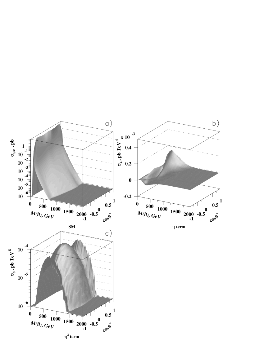
Figure 1: The 3-D plots for double differential distribution $d^{2}\sigma/dM_{\ell\ell}d\cos\theta^{*}$ for Drell-Yan production at the 2 TeV Tevatron. (a) SM only, (b) the interference term between the SM and the gravity contributions, proportional to $\eta$, and (c) the pure gravity contribution, proportional to $\eta^{2}$. Here $\eta={\cal F}c^{n-1}/M_{S}^{4}$. Note that in (b) linear scale is used in the $z$-axis in order to show the negative $z$ values.

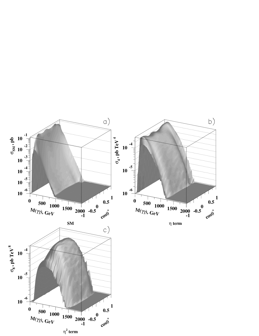
Figure 2: The 3-D plots for double differential distribution $d^{2}\sigma/dM_{\gamma\gamma}d\cos\theta^{*}$ for diphoton production at the 2 TeV Tevatron. (a) SM only, (b) the interference terms between the SM and the gravity contributions, proportional to $\eta$, and (c) the pure gravity contribution, proportional to $\eta^{2}$. Here $\eta={\cal F}c^{n-1}/M_{S}^{4}$.

In Figs. 1 and 2, we show the 3-D plots for the pure SM, the interference, and pure gravity contributions for dilepton and diphoton production, respectively, at the 2 TeV Tevatron. It is clear that the pure SM decreases rapidly with the invariant mass. This is in contrast with the pure gravity contribution that rises quite sharply with the invariant mass and then turns over due to the effect of parton distribution functions. The interference term also shows similar characteristics. The angular distribution also exhibits substantial difference among the pure SM, pure gravity, and the interference. Note the asymmetry of the interference term for dilepton production (Fig. 1b) that arises from the charge asymmetry of the Tevatron beams and final state particles. Analogous distribution for diphotons or in the LHC case is symmetric.

The probability to observe certain set of data ${\cal N}=\{n_{ij}\}$, where $(i,j)$ are the bins in $M$ and $\cos\theta^{*}$, respectively, as a function of $\eta$ is given by the Poisson statistics:

$$P({\cal N}|\eta)=\sum_{ij}\frac{S_{ij}^{n_{ij}}e^{-S_{ij}}}{n_{ij}!},$$ (11)

where $S_{ij}\equiv{\cal L}\epsilon\sigma_{ij}$, and ${\cal L}$ is the integrated luminosity, $\epsilon$ is the identification efficiency, and $\sigma_{ij}$ is the cross section given by Eq. (10), integrated over the bin $(i,j)$.

We now can use Bayes theorem to obtain the probability of $\eta$, given the observed set ${\cal N}$:

$$P(\eta|{\cal N})=\frac{1}{A}\int dx\;\exp\left(\frac{-(x-x_{0})^{2}}{2\sigma_{x}^{2}}\right)\;P({\cal N}|\eta),$$ (12)

where $A$ is the normalization constant, obtained from the unitarity requirement:

$$\int_{0}^{\infty}\;d\eta\;P(\eta|{\cal N})=1\,,$$ (13)

$x_{0}$ is the central value of the $\epsilon{\cal L}$, and $\sigma_{x}$ is the assumed Gaussian error on the quantity $x$. In order to minimize the uncertainty $\sigma_{x}$ we perform in situ calibration by normalizing $x$ to reproduce the observed number of events with $M<100$ GeV (200 GeV) at the Tevatron (LHC) (i.e., we use the first mass bin of the MC grid to perform the normalization). Such a procedure is justified by the fact that possible contribution from Kaluza-Klein gravitons virtually does not affect the low mass region (see Figs. 1 and 2). We, therefore, assume $\sigma_{x}$ to be 10% or $(100\%/\sqrt{\sum_{j}n_{1j}})$, whichever is smaller. (When setting limits on $\eta$ we then only use the mass bins above the normalization region, i.e. $i>1$.)

The 95% C.L. limit on signal, $\eta_{95}$, is obtained from the following integral equation:

$$\int_{0}^{\eta_{95}}d\eta P(\eta|{\cal N})=0.95.$$ (14)

A less sophisticated likelihood approach does ignore systematic error on the efficiency and integrated luminosity and simply treats $P({\cal N}|\eta)$ as the likelihood function. The 95% C.L. limit in this case is obtained by requiring the integral of the likelihood function from the physics boundary ($\eta=0$) to $\eta_{95}$ to be equal to 0.95. As was mentioned before, both approaches yield very close limits on $\eta$. While the Bayesian technique is a natural way to account for the systematic errors on the efficiency (and background) estimates (and this is the approach actually used by the DØ experiment to derive limits), we implemented the classical likelihood approach as well, primarily to demonstrate the robustness of the limit setting technique.

We further combine the results obtained from the dilepton and diphoton channels by adding the probabilities (likelihoods) and solving the integral equation (14) (or its equivalent for the maximum likelihood method).

As an additional cross check we have tested the fitting techniques with a set of the MC experiments assuming a non-zero Kaluza-Klein graviton contribution. Both the Bayesian and maximum likelihood fits were capable of extracting the input value of the gravity scale without a systematic bias, as expected.

To convert $\eta_{95}$ from a single MC experiment into a measure of sensitivity of future experiments, we repeat the above procedures (both the gedankenexperiment and fit) many times. The limits obtained in these repeating experiments are histogrammed. Sensitivity to the parameter $\eta$ is defined as the median of this histogram, i.e. the point on the sensitivity curve which 50% of future experiments will exceed. All the limits given in the next section are based on this sensitivity measure. (An alternative approach that defines sensitivity as the most probable outcome of the gedankenexperiment agrees with the one we used within 5% accuracy.)

4. Results

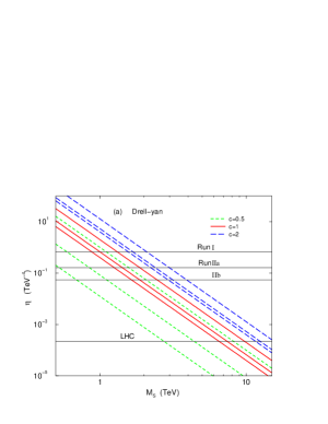
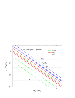
Figure 3: $\eta$ versus $M_{S}$ for a given $(n,c)$. For $c=0.5,1$ the lines from top to bottom are for $n=3,5,7$, whereas for $c=2$ the lines from top to bottom are for $n=7,5,3$. The 95% C.L. limit on $\eta$ for Tevatron Run I, Run II, and for LHC are shown. Limits are based on: (a) Drell-Yan production, (b) diphoton production, and (c) combined.

In our study, we include both the electron and muon channels in the Drell-Yan production. In Table 1 we show the sensitivity to $\eta$ in Run I, Run II of the Tevatron, and at the LHC using dilepton and diphoton production, as well as their combination. Corresponding $M_{S}$ reach is also shown for $n=2-7$ and $c=1$. For other values of $c$ they are shown in Fig. 3 or can be calculated by simple rescaling, using Eq. (8). For the case $n=2$ the conversion of $\eta$ limits into $M_{S}$ limits is not straight-forward, as it depends on the $\hat{s}$ of the subprocess, see Eq. (5). We use the pure gravity contribution in the dilepton and diphoton production to estimate the corresponding average $\hat{s}$. With the average $\hat{s}$ we can then roughly estimate the $M_{S}$ limits for $n=2$. For diphoton production the average $\hat{s}$ for Run I, Run II, and LHC are (0.61 TeV)², (0.66 TeV)², and (3.2 TeV)², respectively, while for dilepton production the average $\hat{s}$ are (0.60 TeV)², (0.64 TeV)², and (3.1 TeV)², respectively.

Table 1: Sensitivity to the low scale gravity model parameter $\eta={\cal F}c^{n-2}/M_{S}^{4}$ in Run I, Run II of the Tevatron and at the LHC, using the dilepton, diphoton production, and their combination. The corresponding 95% C.L. limits on $M_{S}$ are given in TeV for $n=2-7$ and $c=1$. Results for other $c$ values can be read from Fig. 3 or obtained by rescaling, using Eq. (8).

	$\eta_{95}$ (TeV-4)	$n=2$	$n=3$	$n=4$	$n=5$	$n=6$	$n=7$
Run I (130 pb-1)
Dilepton	0.66	1.21	1.32	1.11	1.00	0.93	0.88
Diphoton	0.44	1.39	1.46	1.23	1.11	1.03	0.98
Combined	0.37	1.48	1.53	1.29	1.16	1.08	1.02
Run IIa (2 fb-1)
Dilepton	0.163	1.92	1.87	1.57	1.42	1.32	1.25
Diphoton	0.077	2.40	2.26	1.90	1.71	1.60	1.51
Combined	0.072	2.46	2.30	1.93	1.74	1.62	1.54
Run IIb (20 fb-1)
Dilepton	0.054	2.70	2.47	2.08	1.88	1.75	1.65
Diphoton	0.025	3.40	3.00	2.53	2.28	2.12	2.01
Combined	0.021	3.54	3.11	2.61	2.36	2.20	2.08
LHC (14 TeV, 100 fb-1)
Dilepton	$2.20\times 10^{-4}$	10.2	9.76	8.21	7.42	6.90	6.53
Diphoton	$1.24\times 10^{-4}$	12.1	11.3	9.47	8.56	7.97	7.53
Combined	$1.05\times 10^{-4}$	12.8	11.7	9.87	8.92	8.30	7.85

The Drell-Yan channel is not as sensitive as the diphoton channel and, therefore, the combined limit is close to the limit from the diphoton channel only. In Run I, using the combination of two channels, the sensitivity to $M_{S}$ is about 1.0 to 1.5 TeV for $n=7-2$ and $c=1$. It increases to 1.5 to 2.5 TeV in Run IIa, and 2.1 to 3.5 TeV in Run IIb. At the LHC, the sensitivity soars up to $7.9-12.8$ TeV. Both higher center-of-mass energy and increase in the integrated luminosity help to improve the limits.

We also study the improvement in the sensitivity from the double differential $d^{2}\sigma/dMd\cos\theta^{*}$ fit compared to that from the single differential $d\sigma/dM$ fit. We have repeated the entire procedure with a $20\times 1$ grid in the $(M\times\cos\theta^{*})$ plane, which is equivalent to fitting the single differential distribution $d\sigma/dM$. Corresponding limits in Run IIa deteriorate to:

$$\eta_{95}=0.176\;{\rm TeV}^{-4} \mbox{for dilepton}\;,$$ (15)

$$\eta_{95}=0.089\;{\rm TeV}^{-4} \mbox{for diphoton}\;,$$ (16)

$$\eta_{95}=0.084\;{\rm TeV}^{-4} \mbox{for combined dilepton and diphoton}\;.$$ (17)

By using the double differential cross section we achieve an improvement of about 10% (15%) in the limit on $\eta$ for dileptons (diphotons). While such an improvement in sensitivity translates only into a few per cent increase in the limit on $M_{S}$, it is actually equivalent to a 30% decrease in the integrated luminosity, required to set a certain limit on $M_{S}$.

5. Conclusions

The sensitivity to the effective Planck scale $M_{S}$ obtained in this analysis supercedes those from the previous studies, in which only one-dimensional distributions were used (e.g., Drell-Yan production [5], diboson production [6], diphoton production [7, 8], dijet production and top pair production [9]). The recent work by Éboli et al. [8] that studied diphoton production in the Tevatron Run IIa and at the LHC quotes 95% C.L. upper limits on $M_{S}$ of 1.73 TeV ($n=4$) in Run IIa and 7.7 TeV ($n=4$) at the LHC. Our limits exceeds the latter, partly because we have taken into account the invariant mass and angular distributions simultaneously, and partly because we do not impose the unitarity constraint $\sqrt{\hat{s}}<0.9M_{S}$ and use a slightly higher efficiency.

As we have mentioned in the Introduction, the invariant mass $M$ and the central scattering angle $\cos\theta^{*}$ already span the entire phase space of a $2\to 2$ process. Thus, our fit method gives an ultimate way of probing the low scale gravity in the virtual graviton exchange processes, because all relevant information is contained in the $(M\times\cos\theta^{*})$ plane. We have shown that the improvement in the limits of $\eta$ from the double differential $d^{2}\sigma/dMd\cos\theta^{*}$ fit over those from the single differential $d\sigma/dM$ fit is about 15%, which corresponds to a 30% decrease in the integrated luminosity needed to obtain a certain sensitivity in $M_{S}$.

To summarize, we have analyzed the double differential distribution in the invariant mass and scattering angle for dilepton and diphoton production at hadron colliders. We have obtained better sensitivity than previous studies have achieved. Limits that we obtained using the Bayesian approach and maximum likelihood method are numerically identical. The expected limits on $M_{S}$ are: $0.9-1.5$ TeV (Run I), $1.3-2.5$ TeV (Run IIa), $1.7-3.5$ TeV (Run IIb), and $6.5-12.8$ TeV (LHC) for $n=7-2$.

References

- [1] P. Horava and E. Witten, Nucl. Phys. B460, 506 (1996); ibid., B475, 94 (1996); E. Witten, ibid. B471, 135 (1996); I. Antoniadia, Phys. Lett. B246, 377 (1990); J. Lykken, Phys. Rev. D 54, 3693 (1996); G. Shiu and S. Tye, Phys. Rev. D 58, 106007 (1998); I. Antoniadis and C. Bachas, Phys. Lett. B450, 83 (1999).
- [2] N. Arkani-Hamed, S. Dimopoulos, G. Dvali, Phys. Lett. B429, 263 (1998); I. Antoniadis, N. Arkani-Hamed, S. Dimopoulos, and G. Dvali, Phys. Lett. B436, 257 (1998); N. Arkani-Hamed, S. Dimopoulos, G. Dvali, Phys. Rev. D 59, 086004 (1999); N. Arkani-Hamed, S. Dimopoulos, J. March-Russell, SLAC-PUB-7949, e-Print Archive: hep-th/9809124.
- [3] S. Cullen and M. Perelstein, Phys. Rev. Lett. 83, 268 (1999); L. Hall and D. Smith, LBNL-43091, e-Print Archive: hep-ph/9904267; V. Barger, T. Han, C. Kao, and R.J. Zhang, MADPH-99-1118, e-Print Archive: hep-ph/9905474; A. Pilaftsis, CERN-TH/99-167, e-Print Archive: hep-ph/9906265.
- [4] G. Giudice, R. Rattazzi, and J. Wells, Nucl. Phys. B544, 3 (1999); S. Nussinov and R. Shrock, Phys. Rev. D 59, 105002 (1999); E. Mirabelli, M. Perelstein, and M. Peskin, Phys. Rev. Lett. 82, 2236 (1999); T. Han, J. Lykken, and R. Zhang, Phys. Rev. D 59, 105006 (1999); J. Hewett, Phys. Rev. Lett. 82, 4765 (1999); T. Rizzo, Phys. Rev. D 59, 115010 (1999); Z. Berezhiani and G. Dvali, Phys. Lett. B450, 24 (1999); K. Agashe and N. Deshpande, Phys. Lett. B456, 60 (1999); M. Graesser, LBNL-42812, e-Print Archive: hep-ph/9902310; K. Cheung and W.-Y. Keung, UCD-HEP-99-6, e-Print Archive hep-ph/9903294; T. Rizzo, Phys. Rev. D 60, 075001 (1999); D. Atwood, S. Bar-Shalom, and A. Soni, AMES-HET 99-03, e-Print Archive: hep-ph/9903538; C. Balázs, H.-J. He, W. Repko, C. Yuan, and D. Dicus, e-Print Archive: hep-ph/9904220; G. Shiu, R. Shrock, and S. Tye, Phys.Lett. B458, 274 (1999); K. Lee, H. Song, J. Song, SNUTP-99-021, e-Print Archive: hep-ph/9904355; T. Rizzo, SLAC-PUB-8114, e-Print Archive: hep-ph/9904380; H. Davoudiasl, SLAC-PUB-8121, e-Print Archive: hep-ph/9904425; K. Yoshioka, KUNS-1569, e-Print Archive: hep-ph/9904433; K. Lee, H. Song, J. Song, C. Yu, SNUTP 99-022, e-Print Archive: hep-ph/9905227; X. He, e-Print Archive: hep-ph/9905295; P. Mathews, P. Poulose, and K. Sridhar, TIFR/TH/99-20, e-Print Archive: hep-ph/9905395; T. Han, D. Rainwater, and D. Zeppenfeld, MADPH-99-1115, e-Print Archive: hep-ph/9905423; X. He, e-Print Archive: hep-ph/9905500; A. Das and O. Kong, UR-1576, e-Print Archive: hep-ph/9907272; Z.K. Silagadze, e-Print Archive: hep-ph/9907328; H. Davoudiasl, SLAC-PUB-8197, e-Print Archive: hep-ph/9907347; R.N. Mohapatra, S. Nandi, A. Perez-Lorenzana, FERMILAB-PUB-99/214-T, e-Print Archive: hep-ph/9907520; A. Ioannisian and A. Pilaftsis, CERN-TH/99-230, e-Print Archive: hep-ph/9907522; P. Das and S. Raychaudhuri, IITK-HEP-99-53, e-Print Archive: hep-ph/9908205; Z.K. Silagadze, e-Print Archive: hep-ph/9908208; H.C. Cheng and K. Matchev, FERMILAB-PUB-99/216-T, e-Print Archive: hep-ph/9908328;
- [5] A. Gupta, N. Mondal, and S. Raychaudhuri, TIFR-HECR-99-02, e-Print Archive: hep-ph/9904234; K. Cheung, UCD-HEP-99-8, e-Print Archive: hep-ph/9904266.
- [6] D. Atwood, S. Bar-Shalom, and A. Soni, BNL-HET-99/13, e-Print Archive: hep-ph/9906400;
- [7] K. Cheung, Phys. Lett. B460, 383 (1999).
- [8] O.J.P. Éboli, T. Han, M.B. Magro, and P.G. Mercadante, e-Print Archive: hep-ph/9908358.
- [9] P. Mathews, S. Raychaudhuri, and K. Sridhar, Phys. Lett. B455, 115 (1999); Phys. Lett. B450, 343 (1999); TIFR/TH/99-13, e-Print Archive: hep-ph/9904232.
- [10] M. Bando, T. Kugo, T. Noguchi, and K. Yoshioka, KUNS-1582, e-Print Archive: hep-ph/9906549.
- [11] I. Antoniadis, K. Benakli, and M. Quirós, CERN-TH/99-128, e-Print Archive: hep-ph/9905311.
- [12] G. Landsberg, Plenary talk presented at SUSY’99 conference, Fermilab, June 1999.