BROOKHAVEN NATIONAL LABORATORY   August, 1999 BNL-HET-99/21   
SUSY MEASUREMENTS AT LHC
Frank E. Paige Physics Department Brookhaven National Laboratory Upton, NY 11973 USA
ABSTRACT If SUSY exists at the TeV scale, finding it at the LHC should be quite easy. The more difficult problem is to separate the various SUSY channels and to measure masses and other parameters. Substantial progress on this has been made within the ATLAS and CMS Collaborations.
Invited talk at the International Workshop on Linear Colliders (LCWS99) (Sitges, Spain, 28 April – 5 May 1999). This manuscript has been authored under contract number DE-AC02-98CH10886 with the U.S. Department of Energy. Accordingly, the U.S. Government retains a non-exclusive, royalty-free license to publish or reproduce the published form of this contribution, or allow others to do so, for U.S. Government purposes.

SUSY MEASUREMENTS AT LHC

If SUSY exists at the TeV scale, finding it at the LHC should be quite easy. The more difficult problem is to separate the various SUSY channels and to measure masses and other parameters. Substantial progress on this has been made within the ATLAS and CMS Collaborations.

1 Introduction

If SUSY exists at TeV scale, it should be quite easy to discover at the LHC. The main problem is not to discover SUSY but to make precise measurements of masses and other parameters so as to understand the SUSY model. Over the last several years, the ATLAS $\!{}^{{\bf?}}$ and CMS $\!{}^{{\bf?}}$ Collaborations have studied potential to make such measurements for minimal SUGRA models, minimal GMSB models, and $R$-parity violating models. What can be achieved depends on the whole pattern of production and decay of SUSY particles and hence is very model dependent. This paper describes a few of the many possibilities.

2 Determination of Masses at SUGRA Point 5

“Point 5” is a minimal SUGRA model with $m_{0}=100\,{\rm GeV}$, $m_{1/2}=300\,{\rm GeV}$, $A_{0}=300\,{\rm GeV}$, $\tan\beta=2.1$, and $\mathop{\rm sgn}\mu=+$. It was chosen to give cold dark matter consistent with $\Omega=1$. For the point there are two characteristic ${\tilde{\chi}}_{2}^{0}$ decays: ${\tilde{\chi}}_{2}^{0}\to{\tilde{\ell}}_{R}^{\pm}\ell^{\mp}\to{\tilde{\chi}_{1}^{0}}\ell^{+}\ell^{-}$ and ${\tilde{\chi}}_{2}^{0}\to{\tilde{\chi}_{1}^{0}}h\to{\tilde{\chi}_{1}^{0}}b\bar{b}$.

The “effective mass”, $M_{\rm eff}=\hbox to0.0pt{\hbox to7.95831pt{\hfil/\hfil}\hss}E_{T}+p_{T,1}+p_{T,2}+p_{T,3}+p_{T,4}$, provides a measure of the hardness of the interaction. The Standard Model background is small with the cuts $N_{\rm jet}\geq 4$ with $p_{T}>100,50,50,50\,{\rm GeV}$; $M_{\rm eff}>400\,{\rm GeV}$; and $\hbox to0.0pt{\hbox to7.95831pt{\hfil/\hfil}\hss}E_{T}>\max(100\,{\rm GeV},0.2M_{\rm eff})$.

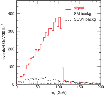
Figure 1: Dilepton mass distribution at Point 5.

If events are also required to have two opposite-sign, same-flavor leptons with ($\ell=e,\mu$) $p_{T}>10\,{\rm GeV}$ and $|\eta|<2.5$, then the decays ${\tilde{\chi}}_{2}^{0}\to{\tilde{\ell}}_{R}\ell$ dominate and produce an endpoint at $\!{}^{{\bf?}}$

$$M_{\ell\ell}^{\rm max}=M_{{\tilde{\chi}}_{2}^{0}}\sqrt{1-{M_{{\tilde{\ell}}_{R}}^{2}\over M_{{\tilde{\chi}}_{2}^{0}}^{2}}}\sqrt{1-{M_{{\tilde{\chi}_{1}^{0}}}^{2}\over M_{{\tilde{\ell}}_{R}}^{2}}}=108.93\,{\rm GeV}.$$

This is clearly seen in Figure 1. Forming the combination $e^{+}e^{-}+\mu^{+}\mu^{-}-e^{\pm}\mu^{\mp}$ removes the remaining small background from two independent decays and allows the endpoint to be measured to about 0.1% at high luminosity. The measurement is sensitive to any $\tilde{e}_{R}-\tilde{\mu}_{R}$ mass difference at a similar level.

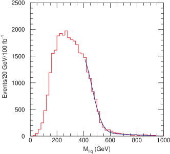
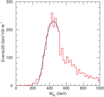
Figure 2: Left: Smaller of the two $\ell\ell q$ masses at Point 5 and a fit used to determine the upper limit from squark decay. Right: Larger of the two $\ell\ell q$ masses with a $\ell\ell$ mass cut and fit used to determine the lower limit from squark decay.

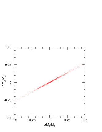
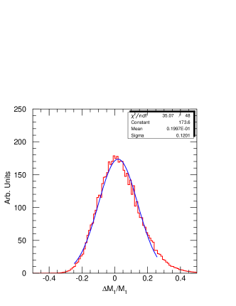
Figure 3: Left: Scatter plot of deviations of masses from their nominal values at Point 5. Right: Projection on the $M_{{\tilde{\chi}_{1}^{0}}}$ axis.

The main source of dileptons is the decay chain ${\tilde{q}}_{L}\to{\tilde{\chi}}_{2}^{0}q\to{\tilde{\ell}}_{R}^{\pm}\ell^{\mp}q\to{\tilde{\chi}_{1}^{0}}\ell^{+}\ell^{-}q$. Four-body phase space gives an $\ell\ell q$ endpoint and an $\ell q$ endpoint with functional forms similar to $M_{\ell\ell}^{\rm max}$. These can be measured by plotting the smaller $\ell\ell q$ mass using the two hardest jets, and then by plotting the $\ell q$ mass for events with only one $\ell\ell q$ mass below $600\,{\rm GeV}$. The $\ell\ell q$ mass distribution is shown in Figure 2 together with a fit used to extract the position of the edge. While the resolutions is only $\sim 10\%$, it is possible to fit these edges with good precision. However, there are not enough constraints to determine all the masses involved. If a lower limit is set on the $\ell\ell$ mass, $M_{\ell\ell}>M_{\ell\ell}^{\rm max}/\sqrt{2}$, then there is also a lower limit on the $\ell\ell q$ mass. This can be measured by plotting the larger of the two masses formed by the $\ell\ell$ pair and one of the two hardest jets; see Figure 2. A fit with the resolution constrained to that obtained in the other jet measurements gives $M_{\ell\ell q}^{\rm min}=283.7^{+4.4}_{-4.5}\,{\rm GeV}$.

By combining all these measurements the ${\tilde{q}}_{L}$, ${\tilde{\chi}}_{2}^{0}$, ${\tilde{\ell}}_{R}$, and ${\tilde{\chi}_{1}^{0}}$ masses can all be determined using only kinematics.$\!{}^{{\bf?}}$ The masses are highly correlated, as can be seen in the scatter plot in Figure 3. The projection of this scatter plot, also shown in Figure 3, determines the ${\tilde{\chi}_{1}^{0}}$ mass to about 12%, assuming a 2% error on the $\ell\ell q$ lower edge. A fit of these measurements to the minimal SUGRA model gives very small errors: $m_{0}=100.0\pm 1.4\,{\rm GeV}$ (1.4%), $m_{1/2}=300.0\pm 2.7\,{\rm GeV}$ (0.9%), $\tan\beta=2.00\pm 0.11$ (5.5%), and $\mu=+1$. However, $A_{0}$ is not constrained — the weak scale $A_{t}$ is insensitive to it. Also, if one allows the $\underline{5}$ and $\underline{10}$ scalar masses to be different at the GUT scale, then the $\underline{5}$ mass is also poorly constrained: it is hard to measure $\ell_{L}$ at the LHC. This is an obvious place where a future linear collider could contribute.

3 $\tau$ Signatures for large $\tan\beta$

For $\tan\beta\mathrel{\hbox to0.0pt{\raise 2.20013pt\hbox{$<$}\hss}{\lower 2.20013pt\hbox{$\sim$}}}10$ usually have at least one of ${\tilde{\chi}}_{2}^{0}\to{\tilde{\chi}_{1}^{0}}\ell^{+}\ell^{-}$, ${\tilde{\ell}}^{\pm}\ell^{\mp},$ or ${\tilde{\chi}_{1}^{0}}h$ is generally available. But for $\tan\beta\gg 1$ the only allowed two-body decay, and hence the dominant decay, may be ${\tilde{\chi}}_{2}^{0}\to{\tilde{\tau}}_{1}^{\pm}\tau^{\mp}\to{\tilde{\chi}_{1}^{0}}\tau^{+}\tau^{-}$. “Point 6” is a minimal SUGRA point with $m_{0}=200\,{\rm GeV}$, $m_{1/2}=200\,{\rm GeV}$, $A_{0}=0$, $\tan\beta=45$, and $\mathop{\rm sgn}\mu=-$ for which this is the case.

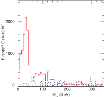
Figure 4: Visible $\tau\tau$ mass distribution at Point 6 after cuts.

A clean sample of SUSY events can be selected with multi-jet, $M_{\rm eff}$, and $\hbox to0.0pt{\hbox to7.95831pt{\hfil/\hfil}\hss}E_{T}$ like those above. An algorithm to reconstruct $\tau$ hadronic decays with tracking and electromagnetic calorimetry was developed using the full simulation of ATLAS.$\!{}^{{\bf?}}$ This algorithm is biased towards high-mass decays to optimize the $\tau\tau$ mass measurement rather than $\tau$ identification. It gives $\langle M_{\rm visible}\rangle=0.66M_{\tau\tau}$ with $(\sigma/M)_{\rm visible}=0.12$. The rejection factor for light jets is about 15. The $\tau^{+}\tau^{-}-\tau^{\pm}\tau^{\pm}$ mass distribution is shown in Figure 4. If the $\tau$’s could be measured perfectly, there would be a sharp edge like that in Figure 1 at $59.64\,{\rm GeV}$. While the edge is smeared, a clear structure remains. The position of this edge can be determined to an estimated $3\,{\rm GeV}$ for $10\,{\rm fb^{-1}}$. This can then be used as a starting point for further partial reconstructions.$\!{}^{{\bf?}}$ A case like this one is clearly more difficult and should be studied for linear colliders.

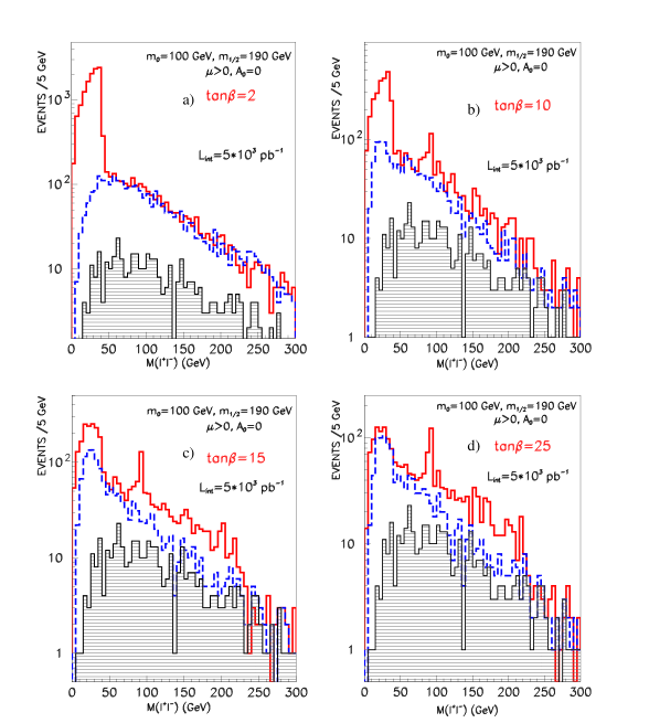
Figure 5: Mass distributions for $e^{+}e^{-}+\mu^{+}\mu^{-}$ (solid) and $e^{\pm}\mu^{\mp}$ (dotted) for various $\tan\beta$.

Decays into $\tau$’s can also be studied by comparing the $e^{+}e^{-}+\mu^{+}\mu^{-}$ and $e^{\pm}\mu^{\mp}$ distributions.$\!{}^{{\bf?}}$ As $\tan\beta$ is increased, the $\tau$ branching ratios become larger, leading to more nearly equal distributions at low mass. This is illustrated in Figure 5, which compares four values of $\tan\beta$ for $m_{0}=100\,{\rm GeV}$, $m_{1/2}=190\,{\rm GeV}$, $A_{0}=0$, and $\mathop{\rm sgn}\mu=+$. The mixing between gauginos and Higgsinos also increases, leading to more heavy gaugino decays. These heavy gauginos can decay both into $Z$’s and into ${\tilde{\ell}}^{\pm}\ell^{\mp}$, giving the higher-mass structure in Figure 5.

4 GMSB Models

The phenomenology of GMSB models depends on the nature and lifetime of the NLSP. Prompt ${\tilde{\chi}_{1}^{0}}\to{\tilde{G}}\gamma$ or ${\tilde{\ell}}\to{\tilde{G}}\ell$ decays give longer decay chains and hence more constraints. A long-lived NLSP ${\tilde{\ell}}_{R}$ allows full reconstruction. In this case it is important to reconstruct muon-like tracks with $\beta<1$ and to measure their mass with time of flight or $dE/dx$. A long-lived NLSP ${\tilde{\chi}_{1}^{0}}$ has signatures qualitatively like SUGRA. In this case it is important to search for rare ${\tilde{\chi}_{1}^{0}}\to{\tilde{G}}\gamma$ decays, since these measure the true SUSY breaking scale. The ATLAS EM calorimeter provides good angular measurements for photons and might be sensitive to decay lengths up to $100\,{\rm km}$. All of these are discussed in much more detail in Reference .

5 Status and Outlook

The LHC produces many SUSY channels and a wide variety of signatures involving combinations of $\hbox to0.0pt{\hbox to7.95831pt{\hfil/\hfil}\hss}E_{T}$, jets, heavy flavors, leptons, and $\tau$’s. The main background for these signatures is other SUSY processes, not Standard Model ones. Given the many complex possibilities, it is hard to draw general conclusions, but we reasonably expect to make many precise measurements. It also seems likely that some aspects of SUSY will be difficult to study at the LHC. The linear collider studies should put particular emphasis on those aspects, including heavy Higgs bosons, heavy Higgsinos, sneutrinos and sleptons with $M_{{\tilde{\ell}}}>M_{{\tilde{\chi}}_{2}^{0}}$, and dominant $\tau$ decays.

This work is supported in part by the U.S. Department of Energy under contract DE-AC02-98CH10886.

References

References

- [1] ATLAS Detector and Physics Performance Technical Design Report, Chapter 20 (June 1999) and references therein.
- [2] CMS Note 1998/006 (April 1998).
- [3] I. Hinchliffe, et al., Phys. Rev. D55 (1997) 5520.
- [4] D. Denegri, W. Majerotto, and L. Rurua, hep-ph/9901231,