NORDITA-1999/52 HE hep-ph/9908501 August 30, 1999
Soft Perturbative QCD[1]

Abstract

There are indications of a faith transition in QCD: The strong coupling may freeze at a sufficiently low value to make PQCD relevant even in the confining regime. The properties of PQCD at low $Q^{2}$ depend on the asymptotic field configuration assumed at $t=\pm\infty$. A change in the i$\epsilon$ prescription of the free propagators is equivalent to including quarks and gluons in the initial and final states. Perturbative expansions thus generated are formally as justified as standard PQCD and may turn out to be phenomenologically relevant. I discuss examples of the effects of such propagator modifications in QED and QCD.

]

I The Faith Transition

Comparisons of physical gauge theories with data rely on perturbation theory. In particular, the successful comparisons of perturbative QCD (PQCD) with data on hard processes has established QCD as the correct theory of the strong interaction.

PQCD does not correctly describe soft processes, where quarks get dressed to massive constituent quarks that are confined to hadrons. It is commonly assumed that this physics is related to a strongly coupled non-perturbative sector of QCD. Evidence is, however, building up that this assumption may be wrong. Phenomenological analyses point to a situation where the strong coupling $\alpha_{s}(Q^{2})$ ‘freezes’ for low $Q^{2}$ at a moderate value $\alpha_{s}(0)/\pi=0.14\ldots 0.17$. The insight that the physics of confinement may be described perturbatively has been dubbed the ‘QCD faith transition’ by Dokshitzer [2].

The following examples indicate a close empirical connection between hard and soft processes. PQCD continues to work even at low $Q^{2}$ provided a regularization of the form $Q^{2}\to Q^{2}+Q_{0}^{2}$ is made, where $Q_{0}$ is a hadronic scale.

• DIS scaling. D. Haidt [3] has shown that HERA data on the structure function $F_{2}(x,Q^{2})$ in the range $x\leq.001$ can be fit by the simple function $F_{2}=0.41\log(0.04/x)\log(1+Q^{2}/Q_{0}^{2})$, where $Q_{0}^{2}=0.5\ {\rm GeV}^{2}$, see Fig. 1. This parametrization works for all available $Q^{2}$, $0.1\lesssim Q^{2}/{\rm GeV}^{2}\lesssim 35$, with no sign of a PQCD to NPQCD ‘phase transition’.

  

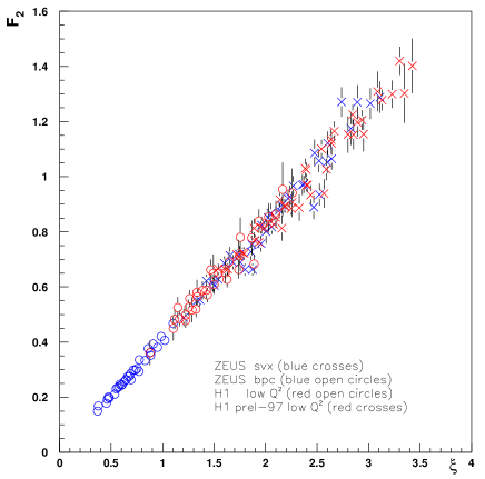
  FIG. 1.: $F_{2}$ data from HERA plotted in terms of the scaling variable $\xi=\log(0.04/x)\log(1+Q^{2}/Q_{0}^{2})$. Figure from Ref. [2].

• Exclusive scaling. Cross sections of exclusive processes obey dimensional scaling down to remarkably low momentum transfers. A striking example is $\sigma(\gamma+d\to p+n)\propto E_{CM}^{22}$ at $\theta_{CM}=89^{\circ}$ for $E_{\gamma}=1\ldots 4$ GeV [4] (see Fig. 2). The PQCD prediction is proportional to $\alpha_{s}^{10}$ and agrees with dimensional scaling only provided the coupling is frozen at low momentum transfers.

  

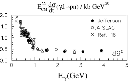
  FIG. 2.: The $\gamma d\to pn$ cross section at $89^{\circ}$ multiplied by $E_{CM}^{22}$ as a function of the photon beam energy [3].

• Local Parton Hadron Duality. The inclusive hadron distribution in $e^{+}e^{-}\to h+X$ and in $eN\to h+X$ appears to faithfully track the inclusive gluon distribution calculated using PQCD, down to momenta of ${\cal O}(200\ {\rm MeV})$ [5].

Fazed by the intriguing possibility that QCD is a weakly coupled theory also in the confinement regime it seems imperative to search for perturbative expansions which can describe data even at low momentum transfers. In the examples above, a hadronic scale was added to standard PQCD ‘by hand’, without theoretical justification.

PQCD is uniquely defined by the QCD lagrangian and by the boundary condition at asymptotic times, $t=\pm\infty$. Formally, the choice of boundary state $|{\Omega_{0}}\rangle$ does not affect the exact all-orders sum, provided that it has an overlap with the true ground state $|{\Omega}\rangle$:

$$\langle\Omega|{\Omega_{0}}\rangle\neq 0\ \ \ \ \Longrightarrow\ \ \ \lim_{t\to\infty(1-i\epsilon\,)}|{\Omega_{0},t}\rangle\propto|{\Omega}\rangle$$ (1)

In standard PQCD we choose $|{\Omega_{0}}\rangle=|{0}\rangle$, the empty ‘perturbative vacuum’. This choice works well in QED. Apparently the true QED vacuum, even though extremely complicated, is sufficiently close to $|{0}\rangle$ for the deviations to be treated perturbatively. The long-distance regime of QCD is, on the other hand, believed to be influenced by a non-trivial ‘gluon condensate’ vacuum [6]. We should then consider other choices for $|{\Omega_{0}}\rangle$, which are sufficiently simple to allow analytic calculations yet are better models of the true QCD ground state than the perturbative vacuum.

Standard PQCD has the elegant feature of being exactly Lorentz covariant at each order of $\alpha_{s}$. S-matrix elements that have free (quark and gluon) asymptotic states manifest their full symmetries at each order of perturbation theory. Conversely, S-matrices whose asymptotic states are bound (hadrons) require infinite orders of $\alpha_{s}$ just to generate the bound state poles. It is unlikely that such resummations can preserve explicit Lorentz covariance at each order of the approximation.

Bound states wave functions are defined on equal time or light-like surfaces. As emphasized by Dirac [7], Lorentz boost generators that do not leave those surfaces invariant have non-trivial representations which involve interactions.

Consider the Fock expansion of the true QCD vacuum (disregarding quarks),

$$|{\Omega}\rangle=\phi_{0}|{0}\rangle+\sum_{n=2}^{\infty}\int\left[\prod_{i}^{n}\frac{d^{3}\mathchoice{{\hbox{\boldmath$\displaystyle p$}}}{{\hbox{\boldmath$\textstyle p$}}}{{\hbox{\boldmath$\scriptstyle p$}}}{{\hbox{\boldmath$\scriptscriptstyle p$}}}_{i}}{(2\pi)^{3}}\right]\,\phi_{n}(\mathchoice{{\hbox{\boldmath$\displaystyle p$}}}{{\hbox{\boldmath$\textstyle p$}}}{{\hbox{\boldmath$\scriptstyle p$}}}{{\hbox{\boldmath$\scriptscriptstyle p$}}}_{i})|{g(\mathchoice{{\hbox{\boldmath$\displaystyle p$}}}{{\hbox{\boldmath$\textstyle p$}}}{{\hbox{\boldmath$\scriptstyle p$}}}{{\hbox{\boldmath$\scriptscriptstyle p$}}}_{1})\cdots g(\mathchoice{{\hbox{\boldmath$\displaystyle p$}}}{{\hbox{\boldmath$\textstyle p$}}}{{\hbox{\boldmath$\scriptstyle p$}}}{{\hbox{\boldmath$\scriptscriptstyle p$}}}_{n})}\rangle$$ (2)

The gluon condensate contributes primarily to the long distance Fock amplitudes $\phi_{n}(|\mathchoice{{\hbox{\boldmath$\displaystyle p$}}}{{\hbox{\boldmath$\textstyle p$}}}{{\hbox{\boldmath$\scriptstyle p$}}}{{\hbox{\boldmath$\scriptscriptstyle p$}}}_{i}|\lesssim\Lambda_{QCD})$. The boost invariance of the ground state,

$$\hat{M}^{0k}|{\Omega}\rangle\propto|{\Omega}\rangle$$ (3)

implies that the condensate appears in the low momentum Fock components $|\mathchoice{{\hbox{\boldmath$\displaystyle p$}}}{{\hbox{\boldmath$\textstyle p$}}}{{\hbox{\boldmath$\scriptstyle p$}}}{{\hbox{\boldmath$\scriptscriptstyle p$}}}_{i}|\lesssim\Lambda_{QCD}$ in all frames. This is possible since the exact boost $\hat{M}^{0k}$ contains interactions. A free boost $\hat{M}_{0}^{0k}$ would simply translate the momenta in each Fock component of Eq. (2), resulting in a very different state.

Describing the boost invariance (3) of the true QCD vacuum is a task of the same magnitude as showing that it is an eigenstate of the exact hamiltonian. Approximate, perturbative calculations satisfy neither exact time translation nor boost invariance. PQCD asymptotic states $|{\Omega_{0}}\rangle$ which contain particles with momenta of ${\cal O}(\Lambda_{QCD})$ will not be invariant even under free boosts.

The general property (1) guarantees exact Lorentz covariance of the full answer, even for non-covariant asymptotic states $|{\Omega_{0}}\rangle$. Only the rate of convergence of the perturbative series may be frame dependent. This can be illustrated for $\alpha_{s}=0$ by choosing $|{\Omega_{0}}\rangle$ to be a superposition of the perturbative vacuum and a state with a gluon of momentum $\textstyle k$,

$$|{\Omega_{0}}\rangle=\phi_{0}|{0}\rangle+\phi_{1}|{g(\mathchoice{{\hbox{\boldmath$\displaystyle k$}}}{{\hbox{\boldmath$\textstyle k$}}}{{\hbox{\boldmath$\scriptstyle k$}}}{{\hbox{\boldmath$\scriptscriptstyle k$}}})}\rangle$$ (4)

This state evolves in time $t$ into

$$e^{-iH_{0}t}|{\Omega_{0}}\rangle=\phi_{0}|{0}\rangle+\phi_{1}e^{-i|\mathchoice{{\hbox{\boldmath$\displaystyle k$}}}{{\hbox{\boldmath$\textstyle k$}}}{{\hbox{\boldmath$\scriptstyle k$}}}{{\hbox{\boldmath$\scriptscriptstyle k$}}}|t}|{g(\mathchoice{{\hbox{\boldmath$\displaystyle k$}}}{{\hbox{\boldmath$\textstyle k$}}}{{\hbox{\boldmath$\scriptstyle k$}}}{{\hbox{\boldmath$\scriptscriptstyle k$}}})}\rangle$$ (5)

The gluon state $|{g(\mathchoice{{\hbox{\boldmath$\displaystyle k$}}}{{\hbox{\boldmath$\textstyle k$}}}{{\hbox{\boldmath$\scriptstyle k$}}}{{\hbox{\boldmath$\scriptscriptstyle k$}}})}\rangle$ is exponentially suppressed wrt. the perturbative vacuum $|{0}\rangle$ in the asymptotic time limit $t\to\infty(1-i\epsilon\,)$.

The above arguments are formal, but so is the justification of standard PQCD. The central point is that it is theoretically justified to consider perturbative expansions with alternative boundary states $|{\Omega_{0}}\rangle$. A choice different from $|{0}\rangle$ is motivated by the known properties of the QCD ground state. The study and interpretation of PQCD for non-trivial $|{\Omega_{0}}\rangle$ is theoretically fascinating and could turn out to be phenomenologically relevant.

II The Perturbative Gluon Condensate

In considering boundary states $|{\Omega_{0}}\rangle$ that might model the gluon condensate, it is instructive to start with perturbation theory in a fermion condensate. Denote the free fermion propagator evaluated between states $|{\bar{f}(\mathchoice{{\hbox{\boldmath$\displaystyle k$}}}{{\hbox{\boldmath$\textstyle k$}}}{{\hbox{\boldmath$\scriptstyle k$}}}{{\hbox{\boldmath$\scriptscriptstyle k$}}},\frac{1}{2})\bar{f}(\mathchoice{{\hbox{\boldmath$\displaystyle k$}}}{{\hbox{\boldmath$\textstyle k$}}}{{\hbox{\boldmath$\scriptstyle k$}}}{{\hbox{\boldmath$\scriptscriptstyle k$}}},-\frac{1}{2})}\rangle$ of two antifermions with 3-momenta $\textstyle k$ and spin $\pm\frac{1}{2}$ by

$$iS_{k}(x-y)\equiv\langle{\bar{f}\bar{f}}|T\{\psi(x)\bar{\psi}(y)\}|{\bar{f}\bar{f}}\rangle/\langle{k}|{k}\rangle^{2}$$ (6)

where $\langle{k}|{k}\rangle=(2\pi)^{3}2E_{k}\delta^{3}(\mathchoice{{\hbox{\boldmath$\displaystyle 0$}}}{{\hbox{\boldmath$\textstyle 0$}}}{{\hbox{\boldmath$\scriptstyle 0$}}}{{\hbox{\boldmath$\scriptscriptstyle 0$}}})$. In momentum space

$$S_{k}(p)=\left\{\begin{array}[]{ll}S_{F}(p)&\ \ \ \ (\mathchoice{{\hbox{\boldmath$\displaystyle p$}}}{{\hbox{\boldmath$\textstyle p$}}}{{\hbox{\boldmath$\scriptstyle p$}}}{{\hbox{\boldmath$\scriptscriptstyle p$}}}\neq-\mathchoice{{\hbox{\boldmath$\displaystyle k$}}}{{\hbox{\boldmath$\textstyle k$}}}{{\hbox{\boldmath$\scriptstyle k$}}}{{\hbox{\boldmath$\scriptscriptstyle k$}}})\\ S_{E}(p)&\ \ \ \ (\mathchoice{{\hbox{\boldmath$\displaystyle p$}}}{{\hbox{\boldmath$\textstyle p$}}}{{\hbox{\boldmath$\scriptstyle p$}}}{{\hbox{\boldmath$\scriptscriptstyle p$}}}=-\mathchoice{{\hbox{\boldmath$\displaystyle k$}}}{{\hbox{\boldmath$\textstyle k$}}}{{\hbox{\boldmath$\scriptstyle k$}}}{{\hbox{\boldmath$\scriptscriptstyle k$}}})\\ \end{array}\right.$$ (7)

where

$$S_{E}(p)=\frac{\parbox[b]{6.00006pt}{$p$}\parbox[b]{5.50003pt}{ \raisebox{-0.86108pt}{$/$}}+m}{(p^{0}-E_{k}+i\epsilon\,)(p^{0}+E_{k}+i\epsilon\,)}$$ (8)

differs from the standard Feynman propagator $S_{F}(p)$ only in the $i\epsilon\,$ prescription at $p^{0}=-E_{k}$. Eq. (7) may also be expressed as

$$S_{k}(p)=S_{F}(p)+i\frac{\parbox[b]{6.00006pt}{$p$}\parbox[b]{5.50003pt}{ \raisebox{-0.86108pt}{$/$}}+m}{\langle{k}|{k}\rangle}(2\pi)^{4}\delta^{4}(p+k)$$ (9)

where $k^{0}=E_{k}$. Filling all antifermion states with $|\mathchoice{{\hbox{\boldmath$\displaystyle k$}}}{{\hbox{\boldmath$\textstyle k$}}}{{\hbox{\boldmath$\scriptstyle k$}}}{{\hbox{\boldmath$\scriptscriptstyle k$}}}|<\Lambda$ gives a propagator that equals $S_{E}(p)$ for all $|\mathchoice{{\hbox{\boldmath$\displaystyle p$}}}{{\hbox{\boldmath$\textstyle p$}}}{{\hbox{\boldmath$\scriptstyle p$}}}{{\hbox{\boldmath$\scriptscriptstyle p$}}}|<\Lambda$.

The equivalence between adding fermions to the boundary states and a change of $i\epsilon\,$ prescription generalizes to Green functions at arbitrary order in perturbation theory [8]:

Any Green function (to arbitrary order in the coupling $\alpha_{s}$) evaluated with the $S_{k}$ fermion propagator gives the same result as a standard calculation using $S_{F}$ with antifermions of momentum $\textstyle k$ added to the initial and final states.

This statement is illustrated in Fig. 3 for the case of a single fermion loop. Modifying the pole prescription of the free propagator for a range of 3-momenta $\textstyle k$ thus allows to include the effect of large number of ‘background’ fermions. The apparent non-causality of the propagation stems from an interference between the background fermions and those propagating (on-shell) in the Green function. The gauge invariance of the standard ($S_{F}$) calculation with external fermions guarantees the gauge invariance of the calculation using $S_{k}$.

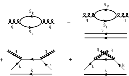
FIG. 3.: A fermion loop calculated with the modified propagator $S_{k}(p)$ is equivalent to a standard calculation using the Feynman propagator $S_{F}(p)$ plus interactions with external antifermions of momentum $k$.

Due to the Pauli principle a fermion condensate prevents the creation of (anti-)fermions with the same momenta as the external ones. In a calculation using $S_{k}$ this is ensured by the $i\epsilon\,$ sign change, which puts both poles of the propagator on the same side of the real axis, thus preventing a pinch.

It seems natural to ask whether a corresponding change of $i\epsilon\,$ sign in boson propagators is also equivalent to standard (Feynman) perturbation theory in the presence of external bosons. This can then serve as a prescription for a ‘perturbative gluon condensate’ $|{\Omega_{0}}\rangle$, which incorporates effects of multiple gluons already at lowest order of PQCD. In particular, such a procedure implies an exclusion principle for bosons, preventing the emission of soft gluons.

As is often the case, the situation for bosons is analogous to that for fermions, with a twist. For a scalar boson that is identical to its antiparticle the Green functions do not depend on whether the sign of $i\epsilon\,$ is changed at the positive or negative energy pole of the propagator. Modifying the prescription at the negative energy pole for a single momentum $\textstyle k$ gives a scalar propagator analogous to Eq. (9)

$$D_{k}(p)=D_{F}(p)+\frac{i}{\langle{k}|{k}\rangle}(2\pi)^{4}\delta^{4}(p+k)$$ (10)

In a realistic application one would change the prescription for a range of momenta, say for $|\mathchoice{{\hbox{\boldmath$\displaystyle k$}}}{{\hbox{\boldmath$\textstyle k$}}}{{\hbox{\boldmath$\scriptstyle k$}}}{{\hbox{\boldmath$\scriptscriptstyle k$}}}|<\Lambda$.

Perturbation theory based on $D_{k}$ is again equivalent to the Feynman ($D_{F}$) one, in the following sense:

Any Green function evaluated (at arbitrary order in the perturbative expansion) using the modified scalar propagator $D_{k}$ is equivalent to a specific superposition of Feynman Green functions with $0,1,2,\ldots$ scalars of momentum $\textstyle k$ in the initial and final states.

A derivation of this, together with the weights for each term in the superposition, may be found in Ref. [8]. There are only diagonal terms, i.e., as many scalars of momentum $\textstyle k$ in the incoming as in the outgoing state. The absence of cross terms means that there is no unique boundary state $|{\Omega_{0}}\rangle$. However, the arguments based on Eq. (1) may be applied to each term in the superposition separately, to show that it generates a formally correct perturbative series. Many of the terms will have non-vanishing total 3-momentum and hence no overlap with the true vacuum – their contributions will be exponentially suppressed as in Eq. (5).

Similar reasoning can be applied to QCD. The perturbative gluon condensate (PGC) proposal [8] is to modify the Feynman gluon propagator at low 3-momenta, $|\mathchoice{{\hbox{\boldmath$\displaystyle p$}}}{{\hbox{\boldmath$\textstyle p$}}}{{\hbox{\boldmath$\scriptstyle p$}}}{{\hbox{\boldmath$\scriptscriptstyle p$}}}|<\Lambda_{QCD}$:

$$D_{\Lambda}^{\mu\nu}(p)=D_{F}^{\mu\nu}(p) - \frac{i\pi g^{\mu\nu}}{2|\mathchoice{{\hbox{\boldmath$\displaystyle p$}}}{{\hbox{\boldmath$\textstyle p$}}}{{\hbox{\boldmath$\scriptstyle p$}}}{{\hbox{\boldmath$\scriptscriptstyle p$}}}|}\left[\delta(p^{0}-|\mathchoice{{\hbox{\boldmath$\displaystyle p$}}}{{\hbox{\boldmath$\textstyle p$}}}{{\hbox{\boldmath$\scriptstyle p$}}}{{\hbox{\boldmath$\scriptscriptstyle p$}}}|)+\delta(p^{0}|+\mathchoice{{\hbox{\boldmath$\displaystyle p$}}}{{\hbox{\boldmath$\textstyle p$}}}{{\hbox{\boldmath$\scriptstyle p$}}}{{\hbox{\boldmath$\scriptscriptstyle p$}}}|)\right]$$ (11)

$$\times \theta(\Lambda_{QCD}-|\mathchoice{{\hbox{\boldmath$\displaystyle p$}}}{{\hbox{\boldmath$\textstyle p$}}}{{\hbox{\boldmath$\scriptstyle p$}}}{{\hbox{\boldmath$\scriptscriptstyle p$}}}|)$$ (12)

This is written in Feynman gauge with the tacit assumption that the contributions from unphysical gluon polarizations and ghosts, which appear as external particles in the equivalent Feynman calculation, cancel among themselves (as they do in internal lines of standard PQCD). A corresponding modification is then required for the ghost propagator,

$$D_{\Lambda}^{ghost}(p)=D_{F}^{ghost}(p) + \frac{i\pi}{2|\mathchoice{{\hbox{\boldmath$\displaystyle p$}}}{{\hbox{\boldmath$\textstyle p$}}}{{\hbox{\boldmath$\scriptstyle p$}}}{{\hbox{\boldmath$\scriptscriptstyle p$}}}|}\,\left[\delta(p^{0}-|\mathchoice{{\hbox{\boldmath$\displaystyle p$}}}{{\hbox{\boldmath$\textstyle p$}}}{{\hbox{\boldmath$\scriptstyle p$}}}{{\hbox{\boldmath$\scriptscriptstyle p$}}}|)+\delta(p^{0}|+\mathchoice{{\hbox{\boldmath$\displaystyle p$}}}{{\hbox{\boldmath$\textstyle p$}}}{{\hbox{\boldmath$\scriptstyle p$}}}{{\hbox{\boldmath$\scriptscriptstyle p$}}}|)\right]$$ (13)

$$\times \theta(\Lambda_{QCD}-|\mathchoice{{\hbox{\boldmath$\displaystyle p$}}}{{\hbox{\boldmath$\textstyle p$}}}{{\hbox{\boldmath$\scriptstyle p$}}}{{\hbox{\boldmath$\scriptscriptstyle p$}}}|)$$ (14)

Averaging over the $i\epsilon\,$ modification at the positive and negative energy poles ensures ghost-antighost symmetry. The same average should be taken in the gluon propagator to satisfy Ward identities.

In the examples of the next section the propagator modifications do, as expected, preserve gauge invariance. It would be important to have an all orders proof of this.

III Examples

The PGC prescription (12), (14) modifies PQCD at low momentum transfers. Due to scattering on the condensate, quarks and gluons get a finite propagation length. Some effort will be required to fully understand and interpret the structure of the modified Green functions. In this section I shall only give some examples of the consequences of the $i\epsilon\,$ modification in QED and QCD.

A Massless QED in 1+1 Dimensions

The Schwinger model [9], alias massless QED in 1+1 dimensions, is exactly solvable. After path integrating the electron field the generating functional

$$Z[J] = \int{\cal D}(A){\rm\exp}\left\{i\int d^{2}x\left[-{1\over 4}F_{\mu\nu}F^{\mu\nu}\right.\right.$$ (15)

$$- \left.\left.{e^{2}\over 2\pi}A_{\mu}(x)\left(-g^{\mu\nu}+{\partial^{\mu}\partial^{\nu}\over\partial^{2}}\right)A_{\nu}(x)+J_{\mu}A^{\mu}\right]\right\}$$ (16)

describes non-interacting photons of mass $e/\sqrt{\pi}$. The mass term is generated by the geometric sum of one-loop corrections to the free photon propagator shown in Fig. 4a,

$$\Pi_{2}^{\mu\nu}(q)=\frac{e^{2}}{\pi}\left(q^{2}g^{\mu\nu}-\frac{q^{\mu}q^{\nu}}{q^{2}}\right)$$ (17)

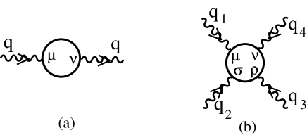
FIG. 4.: Electron loops in $1+1$ dimensional massless QED.

Loops with more than two external photons must vanish for the massive photons to be non-interacting. An explicit calculation of the 4-point loop $\Pi_{4}^{\mu\nu\rho\sigma}$ in Fig. 4b using LC coordinates $q^{\pm}=(q^{0}\pm q^{1})$ shows that it is nonvanishing only for equal $\mu=\nu=\rho=\sigma=\pm$, with

$$\Pi_{4}^{++++}=\frac{4e^{4}}{\pi}\left(\frac{q_{1}^{+}}{q_{2}^{-}q_{23}^{-}q_{234}^{-}}+\frac{q_{12}^{+}}{q_{3}^{-}q_{34}^{-}q_{341}^{-}}+\frac{q_{123}^{+}}{q_{4}^{-}q_{41}^{-}q_{412}^{-}}\right)$$ (18)

Here $q_{ij}\equiv q_{i}+q_{j}$, etc. Summing over the permutations of the external lines one finds that the total contribution of the fermion loop with 4 external photons of arbitrary off-shell momenta $q_{i}$ ($\sum_{i}q_{i}=0$) indeed vanishes.

We may now ask how this situation is changed when the electron propagator is modified as in Eq. (9). For the 2-point function of Fig. 4a the change is

$$\delta_{k}\Pi_{2}^{++}(q)=\frac{4e^{2}}{\langle{k}|{k}\rangle}k^{+}\left(\frac{1}{q^{-}-k^{-}}-\frac{1}{q^{-}+k^{-}}\right)=0$$ (19)

which vanishes due to $k^{+}k^{-}=0$. The modification to the 4-point loop of Fig. 4b similarly vanishes trivially if $k^{+}=0$. For $k^{-}=0$ it is

$$\delta_{k}\Pi_{4}^{++++} = \frac{16e^{4}}{\langle{k}|{k}\rangle}k^{+}\left(\frac{1}{q_{1}^{-}q_{12}^{-}q_{123}^{-}}+\frac{1}{q_{2}^{-}q_{23}^{-}q_{234}^{-}}\right.$$ (20)

$$+ \left.\frac{1}{q_{3}^{-}q_{34}^{-}q_{341}^{-}}+\frac{1}{q_{4}^{-}q_{41}^{-}q_{412}^{-}}\right)=0$$ (21)

The vanishing of the expression in parentheses is most easily seen from its proportionality to the integral

$$\int_{-\infty}^{\infty}\,\frac{dx}{(x+i\epsilon\,)(x+q_{1}^{-}+i\epsilon\,)(x+q_{12}^{-}+i\epsilon\,)(x+q_{123}^{-}+i\epsilon\,)}$$ (22)

When the integration contour is closed in the lower half plane we get the expression in Eq. (21). The integral vanishes since the integrand is analytic in the upper half plane.

I conclude that (at least to ${\cal O}(e^{4})$) the exact Schwinger model solution is unchanged when the electron propagator is modified according to Eq. (9). This example illustrates that the non-covariant modification (9) is compatible with fully Lorentz covariant Green functions.

B Bound States of Weakly Coupled QED₂

Two-dimensional QED simplifies also in the weak coupling limit $m>>e$, where $m$ is the electron mass [10]. Positronium then has no admixture of higher Fock states, since electron loop corrections are suppressed by $e^{2}/m^{2}$ and there are no transverse photons. The bound state dynamics at rest is given simply by the Schrödinger equation. It is, however, interesting to consider the wave function of positronium moving at a relativistic CM velocity.

Since the bound fermions are never on-shell one may, up to loop corrections, alter the $i\epsilon\,$ prescription such that fermions propagate only forward in time. This corresponds to the modification (9) for all momenta $\textstyle k$. One obtains [11] in this way a bound state equation for the equal time wave function

$$\phi_{p}(t;x_{1},x_{2})=e^{-iE_{p}t}\,e^{ip(x_{1}+x_{2})/2}\,\chi_{p}(x_{1}-x_{2})$$ (23)

of two fermions of masses $m_{1,2}$ and CM momentum $p$ of the form

$$- i\left[\gamma^{0}\gamma^{1},\,\frac{\partial}{\partial x}\chi_{p}(x)\right]+\frac{p}{2}\left\{\gamma^{0}\gamma^{1},\,\chi_{p}(x)\right\}$$ (24)

$$+ m_{1}\gamma^{0}\chi_{p}(x)-m_{2}\chi_{p}(x)\gamma^{0}=\left[E_{p}-V(x)\right]\chi_{p}(x)$$ (25)

where $V(x)=e^{2}|x|/2$ is the Coulomb potential.

Eqs. (23) and (25) have no explicit Lorentz covariance, since the wave function is defined at equal time in all frames. Thus the dependence of the energy eigenvalue $E_{p}$ on the CM momentum parameter $p$ is in general not simple. However, it turns out that precisely (and only) for the case of a linear potential Eq. (25) implies $E_{p}=\sqrt{p^{2}+M^{2}}$, with $M$ being the positronium rest mass.

This example serves as another reminder that non-covariant equations can have Lorentz covariant solutions. Although the covariance of Eq. (25) holds for arbitrary coupling, it is only in the weak coupling limit $e/m_{1,2}\to 0$ that loop corrections are suppressed and Eqs. (23), (25) can describe positronium in $1+1$ dimensions. In this limit the rest frame $(p=0)$ equation reduces to the non-relativistic Schrödinger equation, and the wave function $\chi_{p}(x)$ Lorentz contracts with increasing $p$.

C Scalar QED in 3+1 Dimensions

Scalar QED offers an opportunity for studying the effect of the boson propagator modification (10) on perturbation theory in a setting that has many similarities with PQCD. Defining the photon self-energy correction $\Pi(q)$ through

$$\Pi^{\mu\nu}(q)=\left(q^{2}g^{\mu\nu}-q^{\mu}q^{\nu}\right)\Pi(q)$$ (26)

the one-loop result using Feynman propagators is

$$\Pi_{F}(q)=\frac{\alpha}{8\pi}\int_{0}^{1}dx\sqrt{1-x}\log\left(1-\frac{q^{2}x}{4m^{2}}\right)$$ (27)

The modified propagator (10) gives a two-point function $\Pi_{k}^{\mu\nu}(q)$ which differs from the one obtained using Feynman propagators by

$$\Delta_{k}\Pi^{\mu\nu}(q)=\frac{e^{2}}{\langle{k}|{k}\rangle}\sum_{\sigma=\pm 1}\left[\frac{(2k+\sigma q)^{\mu}(2k+\sigma q)^{\nu}}{q^{2}+2\sigma k\cdot q}-g^{\mu\nu}\right]$$ (28)

The contribution from the product of $\delta$-functions has been left out in Eq. (28). At the exceptional values of $q$ where both propagators are modified at the same loop momentum the loop integral vanishes, since all $i\epsilon\,$’s have the same sign.

The modification (28) is readily seen to satisfy the gauge invariance condition $q_{\mu}\Delta_{k}\Pi^{\mu\nu}(q)=0$. Without loss of generality we may take $\textstyle q$ along the 3-axis, $q=(q^{+},q^{-},\mathchoice{{\hbox{\boldmath$\displaystyle 0$}}}{{\hbox{\boldmath$\textstyle 0$}}}{{\hbox{\boldmath$\scriptstyle 0$}}}{{\hbox{\boldmath$\scriptscriptstyle 0$}}}_{\perp})$, with $q^{\pm}=q^{0}\pm q^{3}$. Gauge invariance then constrains $\Pi^{\mu\nu}$ to the form (26) for $\mu,\nu=\pm$, even without assuming Lorentz invariance. One finds,

$$\Delta_{k}\Pi_{L}=\frac{2e^{2}}{\langle{k}|{k}\rangle}\frac{4(m^{2}+k_{\perp}^{2})-q^{2}}{q^{4}-4(q\cdot k)^{2}}$$ (29)

where the subscript $L$ indicates that $\Delta_{k}\Pi_{L}$ refers to Eqs. (26), (28) for $\mu,\nu=\pm$ only. The transverse ($i,j=1,2$) components of Eq. (28) give

$$\Delta_{k}\Pi^{ij}=\frac{2e^{2}}{\langle{k}|{k}\rangle}\left(\delta^{ij}+\frac{4k^{i}k^{j}q^{2}}{q^{4}-4(q\cdot k)^{2}}\right)$$ (30)

There are also cross terms $\Delta_{k}\Pi^{\pm,i}\propto k^{i}$. When summed over all directions of $\textstyle k$ as in the PGC case (12) such terms will cancel. For the present discussion it is sufficient to assume that an integral over the transverse direction (azimuthal angle) of $\textstyle k$ is done. This implies $\Delta_{k}\Pi^{\pm,i}=0$ and $\Delta_{k}\Pi^{ij}=-q^{2}\delta^{ij}\Delta_{k}\Pi_{T}$, where

$$\Delta_{k}\Pi_{T}=-\frac{\alpha}{\langle{k}|{k}\rangle}\left[\frac{1}{q^{2}}+\frac{2k_{\perp}^{2}}{q^{4}-4(q\cdot k)^{2}}\right]$$ (31)

The geometric sum of the 1PI contribution (26) gives the photon propagator

$$\Sigma^{\mu\nu}(q)=-\frac{g^{\mu\nu}-q^{\mu}q^{\nu}/q^{2}}{q^{2}}\frac{1}{1-\Pi(q)}$$ (32)

The usual argument that gauge and Lorentz invariance implies a vanishing of the photon mass in perturbation theory follows from Eq. (32) given that $\Pi(q)$ is finite at $q^{2}=0$. This is verified for Feynman propagators from the expression (27).

With the modification (10) the geometric sum must be done separately for the longitudinal and transverse components (which do not mix as explained above). The function $\Pi(q)$ in Eq. (32) then depends on the photon polarization,

$$\Pi_{L}(q) = \Pi_{F}(q)+\Delta_{k}\Pi_{L}(q)$$ (33)

$$\Pi_{T}(q) = \Pi_{F}(q)+\Delta_{k}\Pi_{T}(q)$$ (34)

From Eq. (29) it may be seen that $\Pi_{L}$ is regular at $q^{2}=0$, hence longitudinally polarized photons are massless. However, $\Delta_{k}\Pi_{T}$ of Eq. (31) has a pole at $q^{2}=0$, implying a finite mass for transverse photons. This is an ‘effective’ mass, which depends on the photon momentum $q$. Moreover, it has an imaginary part, as we shall next discuss.

The singularities of loop integrals arise from pinches between propagator poles that have opposite $i\epsilon\,$ prescriptions. For Feynman propagators pinches can occur between positive and negative energy poles, and correspond to particle-antiparticle pair production. A change of $i\epsilon\,$ prescription at the negative energy pole as in Eq. (10) removes some particle-antiparticle production – for fermions this ensures the Pauli exclusion principle. Instead, ‘pseudothreshold’ singularities arise from pinches between two negative energy poles. These correspond to scattering of the propagating photon on the background scalars, analogous to the lower two diagrams of Fig. 3. The pseudothreshold singularities occur at $q^{2}=\pm 2q\cdot k$, i.e., at

$$q^{+}q^{-}=\pm(q^{+}k^{-}+q^{-}k^{+})$$ (35)

This condition has solutions for both $q^{2}>0$ and $q^{2}<0$, with $q^{+}$ and/or $q^{-}$ of order $k^{\pm}$. E.g., for $k^{-}=0$ we have $q^{+}=\pm k^{+}$ and no condition on $q^{-}$.

In the PGC prescription (12) the background gluon momenta are summed over $|\mathchoice{{\hbox{\boldmath$\displaystyle k$}}}{{\hbox{\boldmath$\textstyle k$}}}{{\hbox{\boldmath$\scriptstyle k$}}}{{\hbox{\boldmath$\scriptscriptstyle k$}}}|<\Lambda_{QCD}$ and the pinch singularities (35) turn into cuts. The imaginary part that thus arises in the gluon propagator reflects a finite propagation length of the gluon due to its scattering on the background particles. The physical QCD condensate will similarly disperse gluons. It is reasonable to assume that the true eigenmodes of propagation in the QCD vacuum will be color singlets, which do not suffer arbitrarily soft interactions. This is in fact what is meant by the term ‘color confinement’. The perturbative gluon condensate offers an opportunity for studying these issues.

D A QCD Ward Identity

The effects of modifying the $i\epsilon\,$ prescription of PQCD propagators are similar to those discussed above for scalar QED. In particular, gauge invariance should be exact at each order in $\alpha_{s}$. As discussed in Section II, in covariant gauges it is important to verify that the unphysical polarizations of gluons and ghosts cancel also for particles in the perturbative condensate.

In Feynman gauge the modified gluon and ghost propagators are, following the PGC prescription (12), (14) for a single momentum $k=(|\mathchoice{{\hbox{\boldmath$\displaystyle k$}}}{{\hbox{\boldmath$\textstyle k$}}}{{\hbox{\boldmath$\scriptstyle k$}}}{{\hbox{\boldmath$\scriptscriptstyle k$}}}|,\mathchoice{{\hbox{\boldmath$\displaystyle k$}}}{{\hbox{\boldmath$\textstyle k$}}}{{\hbox{\boldmath$\scriptstyle k$}}}{{\hbox{\boldmath$\scriptscriptstyle k$}}})$,

$$D_{k}^{\mu\nu,ab}(p) = -g^{\mu\nu}\delta^{ab}\left[\frac{1}{p^{2}+i\epsilon\,}+\delta_{k}\right]$$ (36)

$$D_{k}^{ghost,ab}(p) = \delta^{ab}\left[\frac{1}{p^{2}+i\epsilon\,}+\delta_{k}\right]$$ (37)

where

$$\delta_{k}=\frac{i}{2\langle{k}|{k}\rangle}(2\pi)^{4}\left[\delta^{4}(p-k)+\delta^{4}(p+k)\right]$$ (38)

The gluon + ghost loop modification to the gluon propagator is

$$\Delta_{k}\Pi_{g}^{\mu\nu,ab}(q)=\frac{g^{2}C_{G}\delta^{ab}}{\langle{k}|{k}\rangle}$$ (39)

$$\times \sum_{\sigma=\pm 1}\left[\frac{(2k+\sigma q)^{\mu}(2k+\sigma q)^{\nu}+2(g^{\mu\nu}q^{2}-q^{\mu}q^{\nu})}{q^{2}+2\sigma k\cdot q}-g^{\mu\nu}\right]$$ (40)

where as in Eq. (28) I have ignored the contribution from the product of $\delta$-functions, which only contributes at discrete values of $q$.

QCD Ward identitities follow from the requirement that the BRS transformation of Green functions vanish [12]. The two-point function $\langle{0}|T\{\bar{c}_{a}(x_{1})A_{b}^{\mu}(x_{2})\}|{0}\rangle$, where $c$ and $A$ are ghost and gluon fields, respectively, yields the Ward identity

$$\langle{0}|T\left\{\frac{\partial}{\partial x_{1}^{\nu}}A_{a}^{\nu}(x_{1})A_{b}^{\mu}(x_{2})\right\}|{0}\rangle$$ (41)

$$= \langle{0}|T\left\{\bar{c}_{a}(x_{1})\left[\frac{\partial}{\partial x_{2\mu}}\delta_{bc}+gf_{bcd}A_{d}^{\mu}(x_{2})\right]c_{c}(x_{2})\right\}|{0}\rangle$$ (42)

At ${\cal O}(g^{0})$, this is a relation between the free gluon and ghost propagators which is trivially satisfied due to their identical modification $\delta_{k}$ in (37). At ${\cal O}(g^{2})$, the lhs of Eq. (41) vanishes, $q_{\mu}\Delta_{k}\Pi_{g}^{\mu\nu,ab}(q)=0$ is readily verified from Eq. (39). It turns out that the two terms on the rhs of Eq. (41) cancel. Hence the Ward identity remains valid when evaluated using the modified propagators (37).

While this check of QCD gauge invariance is non-trivial, it does not obviate the need for a general proof.

IV Summary

My proposal to consider modifications of the $i\epsilon\,$ prescription in PQCD is unusual. There seems, however, to be good reasons for pursuing such an approach.

• Perturbation theory is a central tool for comparing physical gauge theories with data. The properties of formally equivalent perturbative series, obtained using different asymptotic states at $t=\pm\infty$, thus merit investigation.

• There are phenomenological indications that $\alpha_{s}(Q^{2})$ freezes at low $Q^{2}$. PQCD appears to be relevant even in the confining, long-distance regime.

• Relativistic corrections are indistinguishable from other higher order effects for bound states, since $\alpha_{s}=v/c$. Exact Lorentz covariance is not required at each order of the approximation [13].

• The PGC prescription (12) provides a gauge-invariant framework for studying the influence of background color fields on quark and gluon interactions. All short distance properties of PQCD are preserved.

The QCD ground state is believed to have also a quark condensate, related to the breaking of chiral symmetry [6]. It may thus be interesting to consider asymptotic states $|{\Omega_{0},t=\pm\infty}\rangle$ which contain also $q\bar{q}$ pairs, as a ‘Perturbative Quark Condensate’ model of the true vacuum. The free fermion propagator between states which have a fermion-antifermion pair of momentum $\textstyle k$ differs from the Feynman propagator in the $i\epsilon\,$ prescription at both the positive and negative energy poles (cf. the discussion at the beginning of Section II). An analysis of the type outlined above for gluons should thus be carried out also for quarks.

Acknowledgements I am grateful to the organizers for their invitation to this interesting workshop, and for helpful discussions with S. J. Brodsky, G. W. Carter, C. S. Lam and H. Weigert.

REFERENCES

- [1] Talk given at the workshop on Exclusive and Semi-exclusive Processes at High Momentum Transfer, Jefferson Lab, USA, May 1999. Work supported in part by the EU/TMR contract EBR FMRX-CT96-0008.
- [2] Yu. L. Dokshitzer, Talk at ICHEP 98 (Vancouver), hep-ph/9812252.
- [3] D. Haidt, Talk at DIS 99 (Zeuthen), www.ifh.de/ dis99p /WGROUP1/wg1-32.ps.gz .
- [4] C. Bochna et al., Phys. Rev. Lett. 81 (1998) 4576.
-
[5]
V. A. Khoze and W. Ochs, Int. J. Mod. Phys. A12 (1997)
2949, hep-ph/9701421;
V. A. Khoze, S. Lupia and W. Ochs, Eur. Phys. J. C5 (1998) 77-90, hep-ph/9711392. - [6] M. A. Shifman, A. I. Vainshtein and V. I. Zakharov, Nucl. Phys. B 147 (1979) 385, 448, 519.
- [7] P. A. M. Dirac, Rev. Mod. Phys. 21 (1949) 392.
- [8] P. Hoyer, hep-ph/9610270 and Proc. APCTP-ICTP Int. Conf. in Seoul, Korea (1997), Y. M. Cho and M. Virasoro, Eds., World Scientific (1998), p. 148, hep-ph/9709444.
- [9] J. Schwinger, Phys. Rev. 128 (1962) 2425.
- [10] S. Coleman, Ann. Phys. (N.Y.) 101 (1976) 239.
- [11] P. Hoyer, Phys. Lett. 172B (1986) 101.
- [12] G. Sterman, An Introduction to Quantum Field Theory, Cambridge University Press, 1993.
- [13] W. E. Caswell and G.P. Lepage, Phys. Rev. A18 (1978) 810.