The Case of a WW Dynamical Scalar Resonance within a Chiral Effective Description of the Strongly Interacting Higgs Sector.

J. A. Oller

Departamento de Física Teórica and IFIC
Centro Mixto Universidad de Valencia-CSIC
46100 Burjassot (Valencia), Spain

Abstract

We have studied the strongly interacting $W_{L}W_{L}\rightarrow W_{L}W_{L}$ I=L=0 partial wave amplitude making use of effective chiral Lagrangians. The Higgs boson is explicitly included and the N/D method is used to unitarize the amplitude. We recover the chiral perturbative expansion at next to leading order for low energies. The cases $m_{H}<<4\pi v$ and $m_{H}>>4\pi v$ are considered in detail. It is shown that in the latter situation a state appears with a mass $\lesssim 1$ TeV. This state is dynamically generated through the strong interactions between the $W_{L}$ and is not responsible for the spontaneous electroweak symmetry breaking. However, its shape can be very similar to that of the $m_{H}\lesssim 1$ TeV case, which corresponds to a conventional heavy Higgs boson.

Although the $SU(2)_{L}\otimes U(1)_{Y}$ theory of electroweak interactions is extremely successful, its spontaneous breaking to $U(1)_{em}$ is a controversial aspect. In the so-called standard model (SM) this is accomplished through a Higgs boson which provides a renormalizable way to generate the needed $W$ and $Z$ masses. However, an experimental verification of this mechanism is still lacking. In fact, unveiling the nature of the electroweak symmetry breaking sector is the number one aim at the LHC which could detect the Higgs boson up to a mass $m_{H}\lesssim 1$ TeV, with $m_{H}$ the mass of the Higgs boson.

Making use of an effective theory formalism [1, 2, 3] we will study in this work the strongly interacting Higgs sector, $m_{H}\gtrsim 1$ TeV. Throughout the paper the SM will be considered first. Then, the extension of our conclusions to more general scenarios will be also discussed.

The effective theory formalism is suited to study the strong electroweak Goldstone boson interactions since for energies well above the mass of the weak bosons ($m_{W}\approx 0.1$ TeV) their scattering amplitudes coincide with those of the longitudinal components of the electroweak gauge bosons ($W_{L}$). This is the content of the so-called equivalence theorem [4].

We will consider the class of models in which the symmetry breaking sector has a chiral $SU(2)_{L}\otimes SU(2)_{R}$ symmetry that breaks spontaneously to the diagonal $SU(2)_{L+R}$ subgroup. The latter “custodial” SU(2) is sufficient [5] (but has not been proved necessary) to protect $\rho=\frac{M_{W}^{2}}{M_{Z}^{2}\cos{\theta_{W}}}\simeq 1$ [6]. This symmetry together with the equivalence theorem guarantees also the universal scattering theorems for the strongly interacting $W^{\prime}s$ and $Z^{\prime}s$ [7]. The former symmetry breaking pattern is the one found in the SM for $g^{\prime}=0$, with $g^{\prime}$ the coupling associated to the hypercharge. In the case of chiral perturbation theory ($\chi PT$) [3] one has the same symmetry breaking situation than before but in this case the custodial symmetry is called isospin (I).

We will consider the $\mathcal{O}(p^{2})$ and $\mathcal{O}(p^{4})$ chiral Lagrangians derived in [1, 2]. The equivalence theorem can be reconciled with this low energy expansion [8] as long as we keep just the lowest order in $g$, which is a rather good approximation. Nevertheless, as we are interested only in the scattering of the Goldstone bosons assuming the custodial $SU(2)$ symmetry we only need the following terms:

$${\cal L}_{2} = \frac{v^{2}}{4}<\partial_{\mu}U\partial^{\mu}U^{\dagger}>$$ (1)

$${\cal L}_{4} = L_{1}\,<\partial_{\mu}U\partial^{\mu}U^{\dagger}>^{2}+L_{2}\,<\partial_{\mu}U\partial^{\nu}U^{\dagger}>^{2}$$

where

$$U=\exp(\frac{i\pi^{i}\tau^{i}}{v})$$ (2)

with $\tau^{i}$ the Pauli matrices, $\pi^{i}$ the Goldstone bosons, $v=(\sqrt{2}\,G_{F})^{-1/2}\simeq\frac{1}{4}$ TeV and the symbol $<>$ represents the trace of the matrix inside it.

The Lagrangian given in eq. (1) describes the scattering of massless pions in $\chi PT$ [3] up to $\mathcal{O}(p^{4})$ just by changing $v$ to $f_{\pi}=92.4$ MeV. Keeping in mind the equivalence theorem, we can write the $W_{L}\,W_{L}$ scattering amplitude up to $\mathcal{O}(p^{4})$ from the $\chi PT$ calculation [3] in the chiral limit (massless pions). The result is:

$$A(s,t,u) = \frac{s}{v^{2}}+\frac{15s^{2}+7(t-u)^{2}}{576\pi^{2}v^{4}}+\frac{2}{v^{4}}\left[(4L_{1}^{r}(\mu)+L_{2}^{r}(\mu))s^{2}+L_{2}^{r}(\mu)(t-u)^{2}\right]$$

$$- \frac{1}{96\pi^{2}v^{4}}\left[3s^{2}\log\frac{-s}{\mu^{2}}+t(t-u)\log\frac{-t}{\mu^{2}}+u(u-t)\log\frac{-u}{\mu^{2}}\right]$$

with $L_{i}^{r}(\mu)$ the finite renormalized value of $L_{i}$ at the scale $\mu$ such that

$$L_{i}=L_{i}^{r}(\mu)+\gamma_{i}\,\lambda$$ (4)

where

$$\lambda=\frac{\mu^{d-4}}{16\pi^{2}}\left[\frac{1}{d-4}-\frac{1}{2}(\log(4\pi)+\Gamma^{\prime}(1)+1)\right]$$ (5)

and

$$\gamma_{1} = \frac{1}{12}$$ (6)

$$\gamma_{2} = \frac{1}{6}$$

In deriving eq. (S0.Ex2) from that of [3] we have multiplied by 4 the term with the counterterms $L_{i}^{r}(\mu)$ in order to connect with the work [9] where the counterterms are calculated in the SM for a heavy Higgs. From this work one has:

$$L_{1}^{r}(\mu) = \frac{v^{2}}{8\,m_{H}^{2}}-\frac{1}{16\pi^{2}}\frac{1}{24}\left(\frac{76}{3}-\frac{27\pi}{2\sqrt{3}}-\log\frac{m_{H}^{2}}{\mu^{2}}\right)$$ (7)

$$L_{2}^{r}(\mu) = -\frac{1}{16\pi^{2}}\frac{1}{12}\left(\frac{11}{6}-\log\frac{m_{H}^{2}}{\mu^{2}}\right)$$

If the $L_{i}^{r}(\mu)$ in eq. (S0.Ex2) are substituted by those of eq. (7) one can see that the $\mu$ dependence of $A(s,t,u)$ disappears and the scale is then fixed by $m_{H}$. The resulting amplitude would reproduce the one loop ${\mathcal{O}}(G_{F}\,m_{H}^{2})$ amplitude in the standard model first calculated in refs. [10] and valid for $4\pi v$, $m_{H}>>\sqrt{s}>>m_{W}$.

The term ${\displaystyle{\frac{v^{2}}{8\,m_{H}^{2}}}}$ in $L_{1}^{r}(\mu)$ in eq. (7) comes from the exchange at tree level of the Higgs bosons at $\mathcal{O}(p^{4})$. In fact, the contribution of the tree level Higgs to $A(s,t,u)$ to all orders can be easily calculated and is given by:

$$\frac{s^{2}}{v^{2}(m_{H}^{2}-s)}$$ (8)

The former result up to $\mathcal{O}(p^{4})$ coincides with the contribution of the Higgs boson to $A(s,t,u)$ coming from the term $v^{2}/(8\,m_{H}^{2})$ in $L_{1}^{r}(\mu)$ of eq. (7). We will then make a resummation of counterterms up to an infinite order by replacing the $\mathcal{O}(p^{4})$ Higgs exchange contribution by the result given in eq. (8) with the full propagator. Substituting also the rest of eq. (7) in eq. (S0.Ex2) one finally obtains:

$$A(s,t,u) = \frac{s}{v^{2}}+\frac{s^{2}}{v^{2}(m_{H}^{2}-s)}-\frac{1}{96\pi^{2}v^{4}}\left[s^{2}(50-\frac{27\pi}{\sqrt{3}})+\frac{2}{3}(t-u)^{2}\right]$$

$$- \frac{1}{96\pi^{2}v^{4}}\left[3s^{2}\log\frac{-s}{m_{H}^{2}}+t(t-u)\log\frac{-t}{m_{H}^{2}}+u(u-t)\log\frac{-u}{m_{H}^{2}}\right]$$

We will concentrate in the I=0 S-wave partial amplitude, $T(s)$, the one which corresponds to the Higgs boson. In terms of $A(s,t,u)$ this partial wave is given by:

$$T(s)=\frac{1}{4}\int_{-1}^{1}d\cos{\theta}\left(3\,A(s,t,u)+A(t,s,u)+A(u,t,s)\right)$$ (10)

With this definition elastic unitarity reads for $s>0$:

$${\rm Im}\,{T(s)}=\frac{1}{16\pi}|T(s)|^{2}$$ (11)

or equivalently

$${\rm Im}\,{1/T(s)}=-\frac{1}{16\pi}$$ (12)

Taking into account eqs. (S0.Ex5) and (10) one has:

$$T(s) = \frac{s}{v^{2}}+\frac{3s^{2}}{2v^{2}(m_{H}^{2}-s)}+\frac{m_{H}^{4}}{sv^{2}}\left[\log(1+\frac{s}{m_{H}^{2}})-\frac{s}{m_{H}^{2}}+\frac{s^{2}}{2\,m_{H}^{4}}\right]$$

$$- \frac{s^{2}}{1728\pi^{2}v^{4}}\left[1673-297\sqrt{3}\pi+108\log\frac{-s}{m_{H}^{2}}+42\log\frac{s}{m_{H}^{2}}\right]$$

where we have added and subtracted the $\mathcal{O}(p^{0})$ and $\mathcal{O}(p^{2})$ contributions of $m_{H}^{4}/(s\,v^{2})\log(1+s/m_{H}^{2})$, due to the exchange of the Higgs in the crossed channels. In this way, the fact that any exchange of the Higgs boson begins at $\mathcal{O}(p^{4})$, as it is clear from eq. (8), is explicitly shown.

In order to study the resonance spectrum of the strongly interacting Higgs sector we are going to make an N/D [11] representation of the former chiral perturbative result. In a former work [12], we used this method to study the strong meson-meson scattering including the resonance region, which in this case appears typically for $\sqrt{s}\gtrsim 1$ GeV. In the N/D method a partial wave amplitude is expressed as the quotient of two functions,

$$T(s)=\frac{N(s)}{D(s)}$$ (14)

with the denominator function $\hbox{D}(s)$, bearing the right hand cut or unitarity cut and the numerator function $\hbox{N}(s)$, the left hand cut.

Taking into account eq. (12), $N(s)$ and $D(s)$ will obey the following equations:

$$\begin{array}[]{ll}{\rm Im}\,D(s)={\rm Im}\,T(s)^{-1}\;N=-\frac{1}{16\pi}\,N(s)&s>0\\ {\rm Im}\,D(s)=0&s<0\end{array}$$ (15)

$$\begin{array}[]{ll}{\rm Im}\,N(s)={\rm Im}\,T(s)\;D(s)\equiv{\rm Im}\,T_{Left}\;D(s)&s<0\\ {\rm Im}\,N(s)=0&s>0\end{array}$$ (16)

In ref. [12] we do not include the left hand cut, although some estimations were done. In eq. (S0.Ex6) the left hand cut first appears through the term ${\displaystyle\log\frac{s}{m_{H}^{2}}}$ which acquires an imaginary part for $s<0$. However, in order to reproduce $T(s)$ up to the order calculated in eq. (S0.Ex6), we will consider here the left hand cut in a perturbative way, such that our $N$ function will satisfy eq. (16) up to one loop calculated at $\mathcal{O}(p^{4})$.

When no left hand cut is included one can always take [12]:

$$N(s) = 1$$ (17)

$$D(s) = \widetilde{a}+\sum_{i}\frac{R_{i}}{s-s_{i}}+g(s)\equiv K^{-1}(s)+g(s)$$

where each term of the sum is referred to as a CDD pole [13] and $g(s)$ is given by

$$g(s)=\frac{1}{16\pi^{2}}\left(\log\frac{-s}{m_{H}^{2}}-a\right)$$ (18)

In [12] we prove that the form for $D(s)$ in eq. (17) has enough room to accommodate the exchange in the s-channel of S and P-wave resonances plus polynomials terms. This is exactly the situation we have from eq. (S0.Ex6), when removing those terms, namely, ${\displaystyle{\log\frac{s}{m_{H}^{2}}\hbox{ and }\left[\log(1+\frac{s}{m_{H}^{2}})-\frac{s}{m_{H}^{2}}+\frac{s^{2}}{2\,m_{H}^{4}}\right]}}$ which give rise to the left hand cut.

In eq. (17) elastic unitarity is fulfilled to all orders in the chiral expansion. For $s>16m_{W}^{2}$ we have neglected the multi $W_{L}$ channels, with four or more $W_{L}$. In fact, in eq. (S0.Ex6) only 2$W_{L}$ appear in the loops since the inclusion of 4$W_{L}$ requires at least two loops, which is $\mathcal{O}(p^{6})$.

Expanding $T(s)$ from eq. (17) up to one loop at $\mathcal{O}(p^{4})$ and comparing with eq.(S0.Ex6) without those terms responsible for the left hand cut given above, one has:

$$K-K_{2}^{2}\,g(s)=\frac{s}{v^{2}}+\frac{3s^{2}}{2\,v^{2}(m_{H}^{2}-s)}-\frac{s^{2}}{1728\pi^{2}v^{4}}\left(1673-297\sqrt{3}\pi\right)-\frac{s^{2}}{16\pi^{2}v^{4}}\log\frac{-s}{m_{H}^{2}}$$ (19)

where $K_{2}$ is the $K$ function at $\mathcal{O}(p^{2})$. Hence:

$$K(s)=\frac{s}{v^{2}}+\frac{3s^{2}}{2v^{2}(m_{H}^{2}-s)}-\frac{s^{2}}{1728\pi^{2}v^{4}}\left(1673-297\sqrt{3}\pi+a\right)$$ (20)

In order to take into account the crossed channel contributions present in eq. (S0.Ex6) we write

$$N(s) = 1+\delta N(s)$$ (21)

$$D(s) = K(s)^{-1}+g(s)\left(1+\delta N(s)\right)$$

In this way, the resulting $T(s)=N(s)/D(s)$ I=L=0 partial wave will satisfy unitarity to all orders. Expanding $T(s)$ up to one loop at $\mathcal{O}(p^{4})$ and comparing the result with eq. (S0.Ex6), taking into account also eq. (19), one has:

$$\delta N(s)=K^{-1}(s)\left[-\frac{7s^{2}}{288\pi^{2}v^{4}}\log\frac{s}{m_{H}^{2}}+\frac{m_{H}^{4}}{v^{2}s}\left(\log(1+\frac{s}{m_{H}^{2}})-\frac{s}{m_{H}^{2}}+\frac{s^{2}}{m_{H}^{4}}\right)\right]$$ (22)

Hence, our final amplitude $T(s)$ will read

$$T(s) = \frac{1+\delta N(s)}{K^{-1}(s)+g(s)\left(1+\delta N(s)\right)}$$

$$= \frac{1}{\left[K\left(1+\delta N(s)\right)\right]^{-1}+g(s)}$$

From eqs. (20) and (22) one has:

$$K(s)\left(1+\delta N(s)\right) = \frac{s}{v^{2}}-\frac{s^{2}}{1728\pi^{2}v^{4}}\left(1673-297\sqrt{3}\pi+108\,a+42\,\log\frac{s}{m_{H}^{2}}\right)$$

$$+ \frac{3s^{2}}{2v^{2}(m_{H}^{2}-s)}+\frac{m^{4}}{v^{2}s}\left(\log(1+\frac{s}{m_{H}^{2}})-\frac{s}{m_{H}^{2}}+\frac{s^{2}}{2m_{H}^{4}}\right)$$

In order to have the usual chiral power counting beginning at $\mathcal{O}(p^{2})$ for $N$ and $D$, we multiply both functions at the same time by $K$. This leaves unchanged their ratio, $T(s)$, and their cut structure. Thus, we will have:

$$N(s) = K(s)\left(1+\delta N(s)\right)$$ (25)

$$D(s) = 1+g(s)\,N(s)$$

It is then easy to see that our $N$ function satisfies eq. (16) up to one loop calculated at $\mathcal{O}(p^{4})$. In fact, at this level, ${\rm Im}\,T_{Left}$ is given by the imaginary part of eq. (S0.Ex10). The $D$ function satisfies eq. (15) identically. This expresses that our final amplitude $T(s)$, given in eq. (S0.Ex9), is unitary to all orders.

It is interesting to compare eq. (S0.Ex9) with the Inverse Amplitude Method (IAM) [14] which we have also used with great phenomenological success in the meson-meson scattering [15]. The IAM has been as well used in the strongly interacting Higgs sector in ref. [16, 17, 18]. This method can be obtained easily from eq. (S0.Ex9) as a special case. To see this let us write:

$$N(s)=K(s)(1+\delta N(s))=N_{2}+N_{4}+...$$ (26)

with $N_{2}$ and $N_{4}$ the $\mathcal{O}(p^{2})$ and $\mathcal{O}(p^{4})$ contributions of the left hand side respectively. Then expanding $\left(K(1+\delta N)\right)^{-1}$ we have

$$\frac{1}{K(1+\delta N)}=\frac{1}{N_{2}+N_{4}}=\frac{1}{N_{2}}-\frac{N_{4}}{N_{2}^{2}}+...$$ (27)

Introducing this result in eq. (S0.Ex9), $T(s)$ reads

$$T(s)=\frac{1}{\frac{1}{N_{2}}-\frac{N_{4}}{N_{2}^{2}}+g(s)}=\frac{N_{2}^{2}}{N_{2}-N_{4}+N_{2}^{2}g(s)}=\frac{T_{2}^{2}}{T_{2}-T_{4}}$$ (28)

with $T_{2}$ the $\mathcal{O}(p^{2})$ chiral amplitude and $T_{4}$ the $\mathcal{O}(p^{4})$ contribution, which is given by $N_{4}-N_{2}^{2}g(s)$. The last expression in eq. (28) is the usual way in which the IAM approach for a partial wave amplitude is presented. Thus, the IAM results in our formalism as a special case through the approximation given in eq. (27).

Let us consider first the case $m_{H}<<4\pi v\simeq 3$ TeV. In order to see analytically what is going on, let us note that for $s\lesssim m_{H}^{2}$ the local terms in eq. (S0.Ex10) of $\mathcal{O}(p^{4})$ divided by $(4\pi v)^{2}$ are much smaller than the ones with $m_{H}^{2}$ in the denominator. On the other hand, close to the bare pole, $s\simeq m_{H}^{2}$, the direct exchange in the s-channel of the resonance dominates over their crossed exchanges and hence we will have:

$$K(1+\delta N) \approx \frac{3m_{H}^{4}}{2v^{2}(m_{H}^{2}-s)}\equiv\frac{\alpha^{2}}{m_{H}^{2}-s}$$ (29)

$$T(s) \approx \frac{\alpha^{2}/(2m_{H})}{m_{H}-\sqrt{s}-\frac{i}{32\pi m_{H}}\alpha^{2}}$$

If one considers $\alpha$ as an arbitrary parameter, only for $\alpha^{2}=3m_{H}^{4}/(2v^{2})$ one has the SM.

Eq. (29) corresponds to a Breit-Wigner resonance, coming from the tree level Higgs pole, with a mass $m_{H}$ and a width

$$\Gamma=\frac{\alpha^{2}}{16\pi m_{H}}$$ (30)

For the SM Higgs boson one obtains the lowest order prediction

$$\Gamma=\frac{3m_{H}^{3}}{32\pi v^{2}}$$ (31)

which is much smaller than $m_{H}$ for

$$m_{H}<<4\pi v\sqrt{\frac{2}{3\pi}}\simeq 1.5\hbox{TeV}$$ (32)

In fact, eq. (29) has sense only when $m_{H}<<\Gamma$.

In the former situation, if we applied the IAM method we would obtain for $s\approx m_{H}^{2}$

$$T(s)=\frac{6m_{H}^{4}/(11v^{2})}{\frac{6m_{H}^{2}}{11}-s-i\frac{3m_{H}^{4}}{88\pi v^{2}}}$$ (33)

with corresponds to a Breit-Wigner with a pole at $\sqrt{s}=\sqrt{\frac{6}{11}}m_{H}$ instead of $m_{H}$ as in eq. (29). Thus, the resummation done in eq. (27) for $\left[K(1+\delta N)\right]$ has shifted the tree level pole from $m_{H}\rightarrow\sqrt{\frac{6}{11}}m_{H}\approx 0.74m_{H}$. This possible source of inaccuracy of the IAM was already established in [12]. In the meson-meson scattering this does not occur because of Vector Meson Dominance in the vector channels and the leading role of unitarity together with coupled channels that happens in the resonant scalar channels with I=0, 1 and 1/2 [12].

A much more interesting case occurs for $m_{H}>>4\pi v$. In this case, for $\sqrt{s}\lesssim 4\pi v$, one can only retain in eq. (S0.Ex10) the two first terms so that:

$$K(s)(1+\delta N(s))\approx\frac{s}{v^{2}}-\frac{s^{2}}{16\pi^{2}v^{4}}\left(a+b+\frac{7}{18}\log\frac{s}{m_{H}^{2}}\right)$$ (34)

In the former equation the $\mathcal{O}(p^{2})$ term is independent of the underlying fundamental theory and is fixed by symmetry and the experimental value of $v$. The same happens for the coefficient $7/18$ in front of ${\displaystyle{\log\frac{s}{m_{H}^{2}}}}$ since it is given by loops at $\mathcal{O}(p^{4})$ in the crossed channels with the $\mathcal{O}(p^{2})$ amplitude at the vertices. However, the coefficients $a$ and $b$ depend on the underlying theory although one expects them to be of $\mathcal{O}(1)$ since they are given over the relevant scale coming from loops $4\pi v$ [19]. In the case of the SM one has from eq. (S0.Ex10):

$$b=\frac{1673-297\sqrt{3}\pi}{108}\simeq\frac{1}{2}$$ (35)

However, the coefficient $a$ in eqs. (S0.Ex10) and (34) is not fixed by the $\mathcal{O}(p^{4})$ chiral perturbation result since at this order cancels with the contributions proportional to $a$ from the $g(s)$ function, eq. (18). Substituting eq. (34) in eq. (S0.Ex9), $T(s)$ then reads

$$T(s)\simeq\left[\left(\frac{s}{v^{2}}-\frac{s^{2}}{16\pi^{2}v^{4}}\left(a+b+\frac{7}{18}\log\frac{s}{m_{H}^{2}}\right)\right)^{-1}+\frac{1}{16\pi^{2}}\left(\log\frac{-s}{m_{H}^{2}}-a\right)\right]^{-1}$$ (36)

On the other hand, for $a$ and $b$ of $\mathcal{O}(1)$ and with $s\lesssim 1$ TeV², well below $(4\pi v)^{2}$, the approximation given in eq. (27) is numerically accurate and then we recover the IAM result eq. (28). As a consequence our results from eqs. (S0.Ex9) and eq. (S0.Ex10) coincide in this case with those already derived in [17] making use of the IAM. The most interesting conclusion is that for $m_{H}\rightarrow\infty$ there is a pole in the I=L=0 partial wave amplitude, with a vanishing mass and width as $m_{H}\rightarrow\infty$. Note also that in eq. (28) the dependence on $a$ disappears.

In order to understand properly the previous result one should keep in mind that, in the present case, $m_{H}$ is just a scale [17] below which the only degrees of freedom are the Goldstone bosons. That is, there are no bare resonances (elementary heavy fields) with any quantum numbers and masses below $m_{H}$. Taking this into account, we can compare our result with the ones of ref. [18]. In this reference, the IAM is applied to study the resonance spectrum of the strongly interacting Higgs sector as a function of $L_{1}^{r}(\mu)$ and $L_{2}^{r}(\mu)$ with $\mu=1$ TeV. The case we are considering, $m_{H}>>4\pi v$, corresponds to those values of the $L_{i}^{r}$ such that the underlying theory has not bare resonances below $m_{H}$. For instance, from eq. (7) we see that, for $m_{H}>>4\pi v$ and $\mu=1$ TeV, $L_{1}^{r}$ and $L_{2}^{r}$ are positive and large ($L_{2}^{r}\approx 2L_{1}^{r}$). In fact in ref. [18], for this region of values of the counterterms, one finds low mass and narrow poles with I=L=0 and no resonances in the other channels (I=L=1 and I=2, L=0).

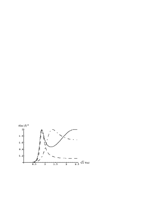
Figure 1: $|T(s)/(16\pi)|^{2}=(\sin\delta(s))^{2}$ where $\delta(s)$ is the phase of $T(s)$, eq. (36). The solid line corresponds to $m_{H}=0.9$ TeV, the dashed line to $m_{H}=150$ TeV and the dotted-dashed line to $m_{H}=11$ TeV. Note as the continuous curve ($m_{H}=0.9$ TeV) is very similar to that with $m_{H}=150$ TeV (dashed line).

In Fig. 1 we show three curves corresponding to $|T(s)/(16\pi)|^{2}=(\sin\delta(s))^{2}$ with $\delta(s)$ the phase of $T(s)$, eq. (S0.Ex9). Three different values for the parameter $m_{H}$ with $b$ given in eq. (35) and $a=1$ are considered. Theses curves are rather stable under changes of $a$ and $b$ of $\mathcal{O}(1)$, for instance, in the interval $[-1,1]$. The solid line is for $m_{H}=0.9$ TeV and one sees for $s\lesssim 1.5$ TeV the presence of a clear resonance located around $m_{H}$, as already discussed above in the case of $m_{H}<<4\pi v$. However, the dashed line, with $m_{H}=150$ TeV, also shows a clear signal for a narrow resonance at 1 TeV and with a shape around the pole position rather similar to that for $m_{H}=0.9$ TeV. This pole with a mass below 1.5 TeV begins to appear for $m_{H}\gtrsim 10$ TeV as already stated in [17]. The dotted-dashed line in fact corresponds to $m_{H}=11$ TeV and one sees clearly a bump corresponding to this pole. However, one has to realize that this state appears without the tree level pole of the Higgs boson, as it is expected from eq. (36) and as we have explicitly checked from eqs. (S0.Ex9) and (S0.Ex10) by removing in the last equation the last line. As a consequence this state does not originate from the tree level Higgs pole and is not a Higgs boson responsible for the spontaneous electroweak symmetry breaking. It is just a consequence of the strong interactions between the $W_{L}$ bosons giving rise to a $W_{L}W_{L}$ resonance, similarly as the deuteron pole is a bound state of a proton and a neutron.

For $m_{H}\approx 4\pi v$ the physics involved is much more dependent on the values of the parameters $a$ and $b$ and both the tree level pole of the Higgs and the rest of counterterms are similarly important and have large interferences. In general, as suggested by eq. (31), the Higgs is very wide, with a width as large or more than its mass. This is in fact what happens for instance for $b$ given by eq. (35), $m_{H}=3$ TeV and $a=0$, where a pole coming from the Higgs tree level pole appears around $(1.2+i\,0.6)$ TeV in the unphysical sheet. However, for certain values of $a$ of $\mathcal{O}(1)$, for instance, $a=-2$ one sees two poles at: $(4+i\,0.04)$ and $(1.2+i\,0.7)$ TeV. As a consequence, the deviations from the light Higgs situation can be very large and simple Breit-Wigner pictures from bare poles are not adequate in this case since the naive formula given in eq. (31) gives a width that for $m_{H}>1.5$ TeV is larger than $m_{H}$. This is a clear signal that the situation cannot be reduced to such simple terms which are valid only for narrow resonances ($\Gamma<<m_{H}$).

In ref. [20] the N/D method is also used to study the strongly interacting Higgs sector. We reproduce their results with a suitable choice of the constant $a$. However, we would like to indicate that while we maintain here the chiral power counting and recover the full chiral amplitude up to $\mathcal{O}(p^{4})$ this is not the case in [20]. Another difference is the way in which the left hand cut is treated. We have included it in a chiral loop expansion while in that reference the left hand cut is fixed a priori to be given by the crossed Higgs exchange.

Conclusions

Making use of the N/D method and the electroweak effective chiral Lagrangians we have studied the properties of the strong $WW$ scattering in the scalar channel. This approach gives rise to physical full unitarized amplitudes respecting the low energy symmetry constraints. In particular, it is able to describe resonances as poles in the unphysical sheet. In this way, we have also played a special attention to the nature of the resonances relevant within the LHC energy range. There are two clearly distinct cases: For $m_{H}<<4\pi v$ the amplitudes are dominated by the tree level Higgs boson pole. For $m_{H}>>4\pi v$, although the previous tree level Higgs pole disappears for the energies considered, there is another physical pole below $\sqrt{s}<1.5$ TeV. The shape of this resonance can be very similar to that of the first case. However, the nature of this second pole is completely different, since it corresponds to a dynamical $WW$ resonance and hence it is not responsible for the spontaneous breaking of the symmetry. We have also seen that this conclusion is stable under changes of the chiral parameters of higher order. Thus, it should be a common feature of any underlying theory responsible for the electroweak symmetry breaking with unbroken custodial symmetry and with heavier particles appearing with a mass $m_{H}>>4\pi v$.

Acknowledgments

I would like acknowledge a critical reading and fruitful discussions with J. R. Peláez, E. Oset and M. J. Vicente-Vacas. This work has been supported by an FPI scholarship of the Generalitat Valenciana and partially by the EEC-TMR Program$-$Contact No. ERBFMRX-CT98-0169.

References

• [1] T. Appelquist and C. Bernard, Phys.Β Rev.Β D22 (1980) 200.
• [2] A. C. Longhitano, Phys.Β Rev.Β D22 (1980) 1166.
• [3] J. Gasser and H. Leutwyler, Ann. Phys. NY 158 (1984) 142.
• [4] J. M. Cornwall, D. N. Levin and G. Tiktopoulos, Phys.Β Rev.Β D10 (1974) 1145; C. E. Vayonakis, Lett. Nuovo. Cim. 17 (1976) 383; B. W. Lee, C. Quigg and H. Thacker, Phys.Β Rev.Β D16 (1977) 1519; M. S. Chanowitz and M. K. Gaillard, Nucl.Β Phys.Β B261 (1985) 379; Y. P. Yao and C. P. Yuan, Phys.Β Rev.Β D38 (1988) 2237.
• [5] P. Sikivie, L. Susskind, M. Voloshin and v. Zakharov, Nucl.Β Phys.Β B173 (1980) 189.
• [6] UA2 Collab., J. Alitti et al., Phys.Β Lett.Β B241 (1990) 150; CDF Collab., F. Abe et al., Phys.Β Rev.Β Lett.Β 65 (1990) 2243.
• [7] M. Chanowitz, M. Golden and H. Georgi, Phys.Β Rev.Β Lett.Β 19 (1986) 2344.
• [8] A. Dobado and J. R. PelΓ‘ez, Nucl.Β Phys.Β B425 (1994) 110; Phys.Β Lett.Β B329 (1994) 469; H. J. He, Y. P. Kuang and X. Li, Phys.Β Lett.Β B229 (1994) 278; A. Dobado, J. R. PelΓ‘ez and M. T. Urdiales, Phys.Β Rev.Β D56 (1997) 7133.
• [9] M. J. Herrero and E. Ruiz Morales, Nucl.Β Phys.Β B418 (1994) 431; Nucl.Β Phys.Β B437 (1995) 319.
• [10] S. Dawson and S. Willenbrock, Phys.Β Rev.Β Lett.Β 62 (1989) 1232; M. J. G. Veltman and F. J. YndurΓ‘in, Nucl.Β Phys.Β B325 (1989) 1.
• [11] G.F. Chew and S. Mandelstam, Phys.Β Rev.Β 119 (1960) 467.
• [12] J. A. Oller and E. Oset, Phys.Β Rev.Β D60 (1999) 074023.
• [13] L. Castillejo, R. H. Dalitz and F. J. Dyson, Phys.Β Rev.Β 101 (1956) 453.
• [14] T. N. Truong, Phys.Β Rev.Β Lett.Β 61 (1988) 2526; $ibid$ 67 (1991) 2260; A. Dobado, M. J. Herrero and T. N. Truong, Phys.Β Lett.Β B235 (1990) 134; J. A. Oller, E. Oset and J. R. PelΓ‘ez, Phys.Β Rev.Β Lett.Β 80 (1998) 3452.
• [15] J. A. Oller, E. Oset and J. R. PelΓ‘ez, Phys.Β Rev.Β D59 (1999) 074001; F. Guerrero and J. A. Oller, Nucl.Β Phys.Β B537 (1999) 459.
• [16] A. Dobado, M. J. Herrero and T. N. Truong, Phys.Β Lett.Β B235 (1990) 129.
• [17] A. Dobado, Phys.Β Lett.Β B237 (1990) 457.
• [18] J. R. PelΓ‘ez, Phys.Β Rev.Β D55 (1997) 4193.
• [19] A. Manohar and H. Georgi, Nucl.Β Phys.Β B234 (1984) 189.
• [20] K. Hikasa and K. Igi, Phys.Β Lett.Β B261 (1991) 285; Phys.Β Rev.Β D48 (1993) 3055.