LBNL-41874

UCB-PTH-98/29

Naturalness and Supersymmetry (Ph.D. Dissertation, University of California, Berkeley, May 1998)
Kaustubh Agashe

Theoretical Physics Group
Lawrence Berkeley National Laboratory
University of California, Berkeley, California 94720
and

Department of Physics
University of California, Berkeley, California 94720

In the Standard Model of elementary particle physics, electroweak symmetry breaking is achieved by a Higgs scalar doublet with a negative (mass)². The Standard Model has the well known gauge hierarchy problem: quadratically divergent quantum corrections drive the Higgs mass and thus the weak scale to the scale of new physics. Thus, if the scale of new physics is say the Planck scale, then correct electroweak symmetry breaking requires a fine tuning between the bare Higgs mass and the quantum corrections.

Supersymmetry, a symmetry between fermions and bosons, solves the gauge hierarchy problem of the Standard Model: the quadratically divergent corrections to the Higgs mass cancel between fermions and bosons. The remaining corrections to the Higgs mass are proportional to the supersymmetry breaking masses for the supersymmetric partners (the sparticles) of the Standard Model particles. The large top quark Yukawa coupling results in a negative Higgs $(\hbox{mass})^{2}$. Thus, electroweak symmetry breaking occurs naturally at the correct scale if the masses of the sparticles are close to the weak scale.

In this thesis, we argue that the supersymmetric Standard Model, while avoiding the fine tuning in electroweak symmetry breaking, requires unnaturalness/fine tuning in some (other) sector of the theory. For example, Baryon and Lepton number violating operators are allowed which lead to proton decay and flavor changing neutral currents. We study some of the constraints from the latter in this thesis. We have to impose an $R$-parity for the theory to be both natural and viable.

In the absence of flavor symmetries, the supersymmetry breaking masses for the squarks and sleptons lead to too large flavor changing neutral currents. We show that two of the solutions to this problem, gauge mediation of supersymmetry breaking and making the scalars of the first two generations heavier than a few TeV, reintroduce fine tuning in electroweak symmetry breaking. We also construct a model of low energy gauge mediation with a non-minimal messenger sector which improves the fine tuning and also generates required Higgs mass terms. We show that this model can be derived from a Grand Unified Theory despite the non-minimal spectrum.

Contents

toc

List of Figures

1. 1.1 The Feynman diagrams which give quadratically divergent contributions to the Higgs mass in the SM.
2. 1.2 The Feynman diagrams in SSM which cancel the quadratic divergences of the SM contributions to the Higgs mass.
3. 1.3 Some of the SUSY contributions to the $\Delta S=2$ four fermion operator. $\tilde{d}(\tilde{s})$ is the scalar partner of left-handed down (strange) quark and $\tilde{d}^{c}(\tilde{s}^{c})$ is the scalar partner of the antiparticle of the right-handed down (strange) quark.
4. 2.1 $\not\!\!R_{p}$ contributions to $K^{0}\!\!-\!\!\bar{K}^{0}$ mixing with one ${\lambda}^{\prime}_{ijk}\neq 0$. Arrows indicate flow of propagating left handed fields.
5. 2.2 $\not\!\!R_{p}\,$ contribution to $K^{+}\rightarrow\pi^{+}\nu\bar{\nu}$ with one ${\lambda}^{\prime}_{ijk}\neq 0$.
6. 3.1 Contours of $c(m^{2}_{Z};\mu^{2})=$(10, 15, 20, 25, 40, 60) for a MSSM with a messenger particle content of one $({\bf 5+\bar{5}})$. In Figs.$(a)$ and $(c)$ $sgn(\mu)=-$1 and in Figs.$(b)$ and $(d)$ $sgn(\mu)=+$1. The constraints considered are: (I) $m_{\tilde{e}_{R}}=$75 GeV , (II) $m_{{\tilde{\chi}}^{0}_{1}}+m_{{\tilde{\chi}}^{0}_{2}}=$ 160 GeV, (III) $m_{\tilde{e}_{R}}=$85 GeV, and (IV) $m_{{\tilde{\chi}}^{0}_{1}}+m_{{\tilde{\chi}}^{0}_{2}}=$ 180 GeV. A central value of $m_{top}=$175 GeV is assumed.
7. 3.2 Contours of $c(m^{2}_{Z};\mu^{2})=$(1, 2, 3, 5, 7, 10) for a MSSM with a messenger particle content of three $(l+\bar{l})$’s and one $(q+\bar{q})$. In Figs.$(a)$ and $(c)$ $sgn(\mu)=-$1 and in Figs.$(b)$ and $(d)$ $sgn(\mu)=+$1. The constraints considered are: (I) $m_{\tilde{e}_{R}}=$75 GeV , (II) $m_{{\tilde{\chi}}^{0}_{1}}+m_{{\tilde{\chi}}^{0}_{2}}=$ 160 GeV, (III) $m_{\tilde{e}_{R}}=$85 GeV, and (IV) $m_{{\tilde{\chi}}^{0}_{1}}+m_{{\tilde{\chi}}^{0}_{2}}=$ 180 GeV. A central value of $m_{top}=$175 GeV is assumed.
8. 3.3 Contours of $c(m^{2}_{Z};\lambda_{H})$ for the NMSSM of section 3.4 and a messenger particle content of three $(l+\bar{l})$’s and one $(q+\bar{q})$. In Figs.$(a)$ and $(b)$, $c(m^{2}_{Z};\lambda_{H})$=(4, 5, 6, 10, 15) and $\lambda_{H}=$0.1. In Figs.$(c)$ and $(d)$, $c(m^{2}_{Z};\lambda_{H})=$(3, 4, 5, 10, 15, 20) and $\lambda_{H}$=0.5. The constraints considered are: 5(I) $m_{h}+m_{a}=m_{Z}$, (II) $m_{\tilde{e}_{R}}=$75 GeV, (III) $m_{{\tilde{\chi}}^{0}_{1}}+m_{{\tilde{\chi}}^{0}_{2}}=$ 160 GeV, (IV) $m_{h}=$ 92 GeV, (V) $m_{\tilde{e}_{R}}=$85 GeV, and (VI) $m_{{\tilde{\chi}}^{0}_{1}}+m_{{\tilde{\chi}}^{0}_{2}}=$ 180 GeV. For $\lambda_{H}=$0.5, the limit $m_{h}\stackrel{{\scriptstyle>}}{{\sim}}$ 70 GeV constrains $\tan\beta\stackrel{{\scriptstyle<}}{{\sim}}$ 5 (independent of $\Lambda_{mess}$) and is thus not shown. A central value of $m_{top}=$175 GeV is assumed.
9. 3.4 Contours of $c(m^{2}_{Z};\lambda_{H})=$(50, 80, 100, 150, 200) for the NMSSM of section 3.4 with $\lambda_{H}=$0.1 and a messenger particle content of one $({\bf 5+\bar{5}})$. The constraints considered are: (I) $m_{h}+m_{a}=m_{Z}$, (II) $m_{\tilde{e}_{R}}=$75 GeV, (III) $m_{{\tilde{\chi}}^{0}_{1}}+m_{{\tilde{\chi}}^{0}_{2}}=$ 160 GeV, (IV) $m_{h}=$92 GeV, (V) $m_{\tilde{e}_{R}}=$85 GeV, and (VI) $m_{{\tilde{\chi}}^{0}_{1}}+m_{{\tilde{\chi}}^{0}_{2}}=$ 180 GeV. A central value of $m_{top}=$175 GeV is assumed.
10. 4.1 Limits for $m_{\tilde{f}_{i},0}/M_{S}$ from the requirement that the (mass)² are positive at the weak scale, for low energy supersymmetry breaking. The regions below the curves are excluded. For the case (2,0), the limits for the other squarks are very similar to that for $\tilde{q}$ and are therefore not shown.
11. 4.2 Limits for $m_{\tilde{t}^{c},0}/M_{S}$ from the requirement that the stop and slepton (mass)² are positive at the weak scale. The regions below the curves are excluded. Low energy gauge mediated supersymmetry breaking and $\tan\beta=$2.2 are assumed.
12. 4.3 Limits for $m_{\tilde{t}^{c},0}$ from the requirement that the stop and slepton (mass)² are positive at the weak scale while suppressing $\Delta m_{K}$, for different values of $(n_{5},n_{10})$, and $(\delta_{LL},\delta_{RR})$. The regions below the curves are excluded. Low energy gauge mediated supersymmetry breaking mass relations and $\tan\beta=$2.2 are assumed.
13. 4.4 Limits for $m_{\tilde{f}_{i},0}$ for different values of $(n_{5},n_{10})$ from the requirement that the (mass)² are positive at the weak scale, assuming a supersymmetry breaking scale of $M_{GUT}$. The allowed region lies above all the lines.
14. 4.5 Limits for $\tilde{m}_{0}/M_{S}$ from the requirement that the stop (mass)² are positive at the weak scale, for $\tan\beta=2.2$, $A_{t,0}=0$ and assuming universal scalar masses at $M_{GUT}$ for the stop and Higgs scalars. The region below the curves are excluded.
15. 4.6 Limits for $m_{\tilde{t},0}/M_{S}$, $m_{\tilde{t}^{c},0}/M_{S}$, from the requirement that the stop (mass)² are positive at the weak scale, for $M_{SUSY}=M_{GUT}$, $\tan\beta=2.2$ and assuming that $m^{2}_{H_{u},0}=0.$ The value of $A_{t,0}$ is chosen to maximize the value of the stop soft masses at the weak scale. The region below the curves are excluded.
16. 4.7 Limits for $m_{\tilde{t},0}/M_{S}$, $m_{\tilde{t}^{c},0}/M_{S}$, from the requirement that the stop (mass)² are positive at the weak scale, for $(n_{5},n_{10})=(2,2)$, $M_{SUSY}=M_{GUT}$, $\tan\beta=2.2$, and different values of $\tilde{\mu}/M_{S}$. The contours end at that value of $M_{3,0}/M_{S}$ that gives $m_{H_{u},0}/M_{S}=0$. The value of $A_{t,0}$ is chosen to maximize the value of the stop soft masses at the weak scale.
17. 4.8 Limits for $m_{\tilde{t},0}$ and $m_{\tilde{t}^{c},0}$, $m_{\tilde{e}^{c}}$, and $m_{\tilde{l}}$ from the requirement that the (mass)² are positive at the weak scale while suppressing $\Delta m_{K}$. It was assumed that $M_{SUSY}=M_{GUT}$, $\tan\beta=2.2$ and that $m^{2}_{H_{u},0}=0.$ The value of $A_{t,0}$ was chosen to maximize the value of the stop soft masses at the weak scale. The heavy scalars were decoupled at the minimum value allowed by $\Delta m_{K}$.
18. 4.9 Limits for $m_{\tilde{t},0}$ and $m_{\tilde{t}^{c},0}$ from the requirement that the stop (mass)² are positive at the weak scale while suppressing $\Delta m_{K}$. It was assumed that $M_{SUSY}=M_{GUT}$, $\tan\beta=2.2$ and that $m^{2}_{H_{u},0}=m^{2}_{\tilde{t}^{c},0}.$ The value of $A_{t,0}$ was chosen to maximize the value of the stop soft masses at the weak scale. The heavy scalars were decoupled at the minimum value allowed by $\Delta m_{K}$.
19. 4.10 Limits for $m_{\tilde{t},0}$ and $m_{\tilde{t}^{c},0}$ from the requirement that the stop (mass)² are positive at the weak scale while suppressing $\Delta m_{K}$, for $(n_{5},n_{10})=(2,2)$, $\sqrt{\delta_{LL}\delta_{RR}}=0.04$, and different values of $\mu$. The contours terminate at $m^{2}_{H_{u},0}=0$. It was assumed that $M_{SUSY}=M_{GUT}$ and $\tan\beta=2.2$. The value of $A_{t,0}$ was chosen to maximize the value of the stop soft masses at the weak scale. The heavy scalars were decoupled at the minimum value allowed by $\Delta m_{K}$.
20. 4.11 Limits for $m_{\tilde{t},0}$, $m_{\tilde{t}^{c},0}$ from the requirement that the stop (mass)² are positive at the weak scale while suppressing $\Delta m_{K}$, for the cases $(n_{5},n_{10})=(2,0)$ and $(0,2)$. It was assumed that $M_{SUSY}=M_{GUT}$, $\tan\beta=2.2$ and that $m^{2}_{H_{u},0}=0.$ The value of $A_{t,0}$ was chosen to maximize the value of the stop soft masses at the weak scale. The heavy scalars were decoupled at the minimum value allowed by $\Delta m_{K}$.
21. B.1 Mixed two loop corrections to the scalar mass. Wavy lines, wavy lines with a straight line through them, solid lines, and dashed lines denote gauge boson, gaugino, fermion and scalar propagators, respectively. The double line denotes the hypercharge $D$-term propagator.

List of Tables

1. 1.1 The particle content of the SM (left column) and it’s supersymmetric extension (the sparticles). The fermions are left-handed Weyl spinors. So, $e^{c}$ stands for the left-handed positron which is the antiparticle of the right-handed electron. $i=1,2,3$ denotes the generation, for example, $u_{3}$ is the top $(t)$ quark and $e^{c}_{2}$ is the anti-muon ($\bar{\mu}$). The electric charge is given by $Q=T_{3}+Y$, where $T_{3}$ is the third component of the $SU(2)_{w}$ isospin and $Y$ is the hypercharge.
2. 2.1 Constraints on $\left|\lambda_{ijk}^{\prime}\right|$ from: (a) $K^{+}\rightarrow\pi^{+}\nu\bar{\nu}$ $(90\%CL)$; (b) $b\rightarrow s\nu\bar{\nu}$ $(90\%CL)$ [55]; (c) $\nu_{e}$ mass $(90\%CL)$ [23]. These constraints were obtained assuming $CKM$-like mixing in the charged $-1/3$ quark sector. All limits are for $100\,\hbox{GeV}$ sparticle masses.
3. 3.1 Soft scalar masses in GeV for messenger particle content of three $(l+\bar{l})$’s and one $q+\bar{q}$ and a scale $\Lambda_{mess}=50$ TeV.
4. 3.2 $SU(5)\times SU(5)^{\prime}\times Z_{3}\times Z^{\prime}_{3}\times Z_{4}$ quantum numbers for the fields of the model discussed in section 3.6. The generators of $Z_{3}\times Z^{\prime}_{3}\times Z_{4}$ are labeled by $(a,b,c)$. The three SM generations are labeled by the index $i$.
5. 4.1 Minimum values for heavy scalar masses $M_{S}$ obtained from the measured value of $\Delta m_{K}$ assuming $M^{2}_{3}/M^{2}_{S}\ll 1$. The limits labeled ‘QCD incl.’ include QCD corrections as discussed in the text. Those labeled as ‘no QCD’ do not.
6. 4.2 Minimum values for heavy scalar masses $M_{S}$ obtained from the measured value of $\Delta m_{K}$ assuming $M^{2}_{3}/M^{2}_{S}\ll 1$. The limits labeled as ‘QCD incl.’ include QCD corrections as discussed in the text. Those labeled as ‘no QCD’ do not. The limits for $(n_{5},n_{10})=(0,2)$ obtained by $\delta_{LL}^{d}\leftrightarrow\delta_{RR}^{d}$ are similar and not shown.

Acknowledgements

I would like to express my sincere gratitude to my advisors, Professor Mahiko Suzuki and Dr. Ian Hinchliffe, for their guidance, help and support. I appreciate the freedom they gave me in choosing research topics. I thank my fellow student, Michael Graesser, for many wonderful collaborations and discussions.

I would also like to thank other members of the Theoretical Physics group, especially Professor Hitoshi Murayama, Nima Arkani-Hamed, Chris Carone, Takeo Moroi, John Terning, Csaba Csáki and Jonathan Feng for useful discussions and the whole group for a pleasant experience of being at LBNL. I am grateful to Anne Takizawa and Donna Sakima of the Physics department and Luanne Neumann, Barbara Gordon and Mary Kihanya at LBNL for help with administrative work.

I am indebted to my roommates and other friends for making my stay at Berkeley thoroughly enjoyable. I thank my parents and my brother for their support and encouragement.

Chapter 1 Introduction

A Standard Model (SM) [1, 2] of elementary particle physics has developed over the last twenty five years or so. It describes the interactions of the elementary particles using gauge theories. The elementary particles are the matter fermions (spin half particles) called the quarks and the leptons, and the gauge bosons (spin one particles) which are the carriers of the interactions. There are three generations, with identical quantum numbers, of quarks and leptons: up ($u$) and down ($d$) quarks, electron ($e$) and it’s neutrino ($\nu$) (the leptons) in the first generation, charm ($c$) and strange ($s$) quarks, muon ($\mu$) and it’s neutrino in the second, and top ($t$) and bottom ($b$) quarks, tau ($\tau$) lepton and it’s neutrino in the third. The $W$, $B$ (the hypercharge gauge boson) and the gluon ($g$) are the gauge bosons. There is also one Higgs scalar. The particle content of the SM is summarized in Table 1.1.

particle	sparticle	$SU(3)_{c}$	$SU(2)_{w}$	$U(1)_{Y}$
$\left(\begin{array}[]{c}u\\ d\\ \end{array}\right)_{i}$	$\left(\begin{array}[]{c}\tilde{u}\\ \tilde{d}\\ \end{array}\right)_{i}$	${\bf 3}$	${\bf 2}$	$\frac{1}{6}$
$u^{c}_{i}$	$\tilde{u}^{c}_{i}$	${\bf\bar{3}}$	${\bf 1}$	$-\frac{2}{3}$
$d^{c}_{i}$	$\tilde{d}^{c}_{i}$	${\bf\bar{3}}$	${\bf 1}$	$\frac{1}{3}$
$\left(\begin{array}[]{c}\nu\\ e\\ \end{array}\right)_{i}$	$\left(\begin{array}[]{c}\tilde{\nu}\\ \tilde{e}\\ \end{array}\right)_{i}$	${\bf 1}$	${\bf 2}$	$-\frac{1}{2}$
$e^{c}_{i}$	$\tilde{e}^{c}_{i}$	${\bf 1}$	${\bf 1}$	$1$
$W$	$\tilde{W}$	${\bf 1}$	${\bf 3}$	$0$
$g$	$\tilde{g}$	${\bf 8}$	${\bf 1}$	$0$
$B$	$\tilde{B}$	${\bf 1}$	${\bf 1}$	$0$
$\left(\begin{array}[]{c}H_{u}^{+}\\ H_{u}^{0}\\ \end{array}\right)$	$\left(\begin{array}[]{c}\tilde{H}_{u}^{+}\\ \tilde{H_{u}^{0}}\\ \end{array}\right)$	${\bf 1}$	${\bf 2}$	$\frac{1}{2}$
$\left(\begin{array}[]{c}H_{d}^{0}\\ H_{d}^{-}\\ \end{array}\right)$	$\left(\begin{array}[]{c}\tilde{H}_{d}^{0}\\ \tilde{H_{d}^{-}}\\ \end{array}\right)$	${\bf 1}$	${\bf 2}$	$-\frac{1}{2}$

Table 1.1: The particle content of the SM (left column) and it’s supersymmetric extension (the sparticles). The fermions are left-handed Weyl spinors. So, $e^{c}$ stands for the left-handed positron which is the antiparticle of the right-handed electron. $i=1,2,3$ denotes the generation, for example, $u_{3}$ is the top $(t)$ quark and $e^{c}_{2}$ is the anti-muon ($\bar{\mu}$). The electric charge is given by $Q=T_{3}+Y$, where $T_{3}$ is the third component of the $SU(2)_{w}$ isospin and $Y$ is the hypercharge.

The gauge theory of the interactions of the quarks, Quantum Chromodynamics (QCD) [3], is based on the gauge group $SU(3)_{c}$ where the “c” stands for “color” which is the charge under QCD in analogy to electric charge. The interaction is mediated by eight massless gauge bosons called gluons. This theory is asymptotically free, i.e., it has the property that it’s gauge coupling becomes weak at high energies (much larger than $\sim 1$ GeV) and becomes strong at energies below $\sim 1$ GeV. Thus, at low energies the theory confines, i.e., the strong interactions bind the quarks into color singlet states called hadrons, for example the proton and the pion. So, we observe only these bound states of quarks and not the elementary quarks. However, when the proton is probed at high energies (large momentum transfers) or when the quarks are produced in high energy collisions, the quarks should behave as if they do not feel the strong interactions. This is indeed confirmed in a large number of experiments at high energies (see, for example, review of QCD in [4]).

The weak and electromagnetic interactions of quarks and leptons are unified into the electroweak theory based on the gauge group $SU(2)_{w}\times U(1)_{Y}$ [1]. This theory has four gauge bosons. This electroweak symmetry is broken to the $U(1)$ of electromagnetism (Quantum Electrodynamics, QED). Three of the gauge bosons (called the $W$ and $Z$ gauge bosons) get a mass in this process whereas the photon (the carrier of electromagnetism) is massless. The theory predicts the relations between the $W$ and $Z$ masses and couplings of quarks and leptons to these gauge bosons. The stringent tests of these predictions at the electron-positron collider at CERN (LEP) and at the proton-antiproton collider at Fermilab (up to energies of a few $100$ GeV) have been highly successful.

One of the central issues of particle physics today is the mechanism of Electroweak Symmetry Breaking (EWSB), i.e., how is $SU(2)_{w}\times U(1)_{Y}$ broken to $U(1)_{em}$? In the SM, this is achieved by the Higgs scalar, $H$, which is a doublet of $SU(2)_{w}$. The Higgs scalar has the following potential:

$$V_{Higgs}=m^{2}\left|H\right|^{2}+\lambda\left|H\right|^{4}.$$ (1.1)

If $m^{2}<0$, then at the minimum of the potential, the Higgs scalar acquires a vacuum expectation value (vev):

$$\langle H\rangle=\left(\begin{array}[]{c}v\\ 0\end{array}\right),$$ (1.2)

where $v=\sqrt{-m^{2}/(2\lambda)}$. Thus two of the generators of the $SU(2)_{w}$ gauge group and also one combination of the third $SU(2)_{w}$ generator and $U(1)_{Y}$ are broken. The corresponding gauge bosons acquire masses given by $\sim g_{2}\;v$ and $\sim\sqrt{g_{2}^{2}+g_{Y}^{2}}\;v$ respectively and are the $W$ and the $Z$. The Higgs vev and thus, if $\lambda\sim O(1)$, the mass parameter $m^{2}$ has to be of the order of ($100$ GeV)² to give the experimentally measured $W$ and $Z$ gauge boson masses. The other combination of the third $SU(2)_{w}$ generator and $U(1)_{Y}$ is still a good symmetry and the corresponding gauge boson is massless and is the photon ($\gamma$). There is also a physical electrically neutral Higgs scalar left after EWSB. This is the only particle of the SM which has not been discovered.

To generate masses for the quarks and leptons, we add the following Yukawa couplings (the quark and lepton $SU(2)_{w}$ doublets are denoted by $q$ and $l$ and $i,j$ are generation indices):

$${\cal L}_{Yukawa}=\lambda^{u}_{ij}Hq_{i}u^{c}_{j}+\lambda^{d}_{ij}H^{\dagger}q_{i}d^{c}_{j}+\lambda^{l}_{ij}H^{\dagger}l_{i}e^{c}_{j},$$ (1.3)

where repeated indices are summed over. These couplings become mass terms for the fermions when the Higgs develops a vev. There are 13 physical parameters in the above Lagrangian: 6 masses for the quarks, 3 masses for the leptons and 3 mixing angles and a phase in the quark sector. The 3 mixing angles and the phase appear at the $W$ vertex involving the quarks and constitute the $3\times 3$ matrix called the Cabibbo-Kobayashi-Maskawa (CKM) matrix [5]. These 13 parameters can be, a priori, arbitrary and are fixed only by measurements of the quark and lepton masses and the mixings (the latter using decays of quarks through a virtual $W$). In the SM, processes involving conversion of one flavor of quark into another flavor with the same electric charge, for example, conversion of a strange quark into a down quark resulting in mixing between the $K$-meson and it’s antiparticle, do not occur at tree level, but occur at one loop due to the mixings. The experimental observations of these flavor changing neutral currents (FCNC’s) are consistent with the mixing angles (as measured using decays of quarks). Since there is no right-handed neutrino in the SM, we cannot write a Dirac mass term for the neutrino and at the renormalizable level, we cannot write a Majorana mass term since we do not have a $SU(2)_{w}$ triplet Higgs. So, neutrinos are massless in the SM. This results in conservation laws for the individual lepton numbers, i.e., electron, muon and tau numbers. Thus, the FCNC decay, $\mu\rightarrow e\;\gamma$ is forbidden in the SM and the experimental limits on such processes are indeed extremely small [4].

The SM, thus, seems to describe the observed properties of the elementary particles remarkably well, up to energies $\sim$ few $100$ GeV. Of course, the Higgs scalar remains to be found. But, the SM has some aesthetically unappealing features which we now discuss.

The SM particle content and gauge group naturally raise the questions: Why are there three gauge groups (with different strengths for the couplings) and three generations of quarks and leptons with the particular quantum numbers? Attempts have been made to simplify this structure by building Grand Unified Theories (GUT’s). The gauge coupling strengths depend on the energy/momentum scale at which they are probed (this was already mentioned for QCD above). In the GUT’s it is postulated that these three couplings are equal at some very high energy scale called the GUT scale so that at that energy scale the three gauge groups can be embedded into one gauge group with one coupling constant. The GUT gauge group gets broken at that scale to the SM gauge groups resulting in different evolutions for the three gauge couplings below the GUT scale. Also, in the GUT’s, the quarks and leptons can be unified into the same representation of the gauge group. In the simplest GUT, based on the $SU(5)$ gauge group [6], the $d^{c}$ and the lepton doublet ($l$) form an anti-fundamental $({\bf\bar{5}})$ under the gauge group. The Higgs doublets are in a ${\bf 5}$ representation of $SU(5)$ and so have $SU(3)_{c}$ triplet partners which are required to be heavy since they mediate proton decay [6]. When the three coupling constants were measured in the late 1970’s, and evolved with the SM particle content to high energies, they appeared to meet at an energy scale of $\sim 10^{14}$ GeV [7]. But, the more accurate measurements in the 1990’s show that this convergence is not perfect [8].

The 13 parameters of the Yukawa Lagrangian of Eqn.(1.3) exhibit hierarchies or patterns, for example the ratio of the mass of the heaviest (top) quark and the lightest lepton (electron) is about $10^{-6}$. One would like to have a more fundamental theory of these Yukawa couplings which can explain these hierarchies in terms of fewer parameters. A GUT can make some progress in this direction by relating the quark masses to the lepton masses since they are in the same representation of the GUT group [6]. For example in many GUT’s we get the relation $m_{b}=m_{\tau}$.

Perhaps the most severe “problem” of the SM is the gauge hierarchy problem [9] which we now explain. It concerns the Higgs mass parameter, $m^{2}$, of Eqn.(1.1). There are two issues here. The first issue is the origin of this mass parameter. As mentioned above, $m^{2}\sim(100$ GeV)². We would like to have one “fundamental” mass scale in our theory and “derive” all other mass scales from this scale. Particle physicists like to think that this scale should be the Planck scale, $M_{Pl}\sim 10^{18}$ GeV, which is the scale at which the gravitational interactions have to be quantized. There is one other scale in the SM besides the Higgs mass parameter. It is the strong interaction scale of QCD denoted by $\Lambda_{QCD}$. Naively, this is the scale at which the $SU(3)_{c}$ coupling constant becomes strong binding quarks into hadrons. Thus, this scale can be related to the Planck scale and the $SU(3)_{c}$ coupling constant at the Planck scale by the logarithmic Renormalization Group (RG) evolution of the gauge coupling as follows:

$$\Lambda_{QCD}\sim M_{Pl}\exp\left(-\frac{8\pi^{2}}{g^{2}(M_{Pl})}\right).$$ (1.4)

This relation is valid, strictly speaking, at one loop. Thus, if $g(M_{Pl})\raisebox{-1.72218pt}{\hbox to0.0pt{$\sim$\hss}}\raisebox{1.72218pt}{$<$}1$, there is a natural explanation for the hierarchy $\Lambda_{QCD}/M_{Pl}$. We would like to have a similar explanation for the hierarchy $m/M_{Pl}$.

Figure 1.1: The Feynman diagrams which give quadratically divergent contributions to the Higgs mass in the SM.

The second issue is whether the mass scale $m$ is stable to quantum corrections. In the SM, the Feynman diagrams in Fig.1.1 give quadratically divergent contributions to $m^{2}$, since the corresponding integrals over the loop momentum $k$ are $\sim\int d^{4}k/(k^{2}-m^{2})$. The corrections due to the top quark in the loop are important due to the large Yukawa coupling of the top quark. Thus, the renormalized Higgs mass parameter is given by:

$$m^{2}_{ren.}\sim m^{2}_{bare}+\frac{1}{16\pi^{2}}\Lambda^{2},$$ (1.5)

for all dimensionless couplings of order one. $\Lambda$ is the cut-off for the quadratically divergent integral. We know that the SM cannot describe quantum gravity. Thus, we certainly expect some new physics (string theory?) at $M_{Pl}$. There could, of course, be some new physics at lower energy scales as well, for example the GUT scale. In some such extension to the SM, it turns out that the scale $\Lambda$ is the scale of new physics. Thus, in the SM, the Higgs mass gets driven due to quantum corrections all the way to some high energy scale of new physics (see Eqn.(1.5)). We need $m^{2}_{ren.}\sim(100$ GeV$)^{2}$ so that EWSB occurs correctly. We can achieve this by a cancellation between $m^{2}_{bare}$ and the quantum corrections, which is of the order of one part in $\Lambda^{2}/(100$ GeV$)^{2}$. For $\Lambda=M_{Pl}$, this is enormous. Thus, in the SM, the bare Higgs mass parameter has to be fine tuned to give the correct $W$ and $Z$ masses. Such a problem does not occur for dimensionless couplings, since the quantum corrections are proportional to the logarithm of the cut-off or for fermion masses which are protected by chiral symmetries.

Supersymmetry (SUSY) [10] provides a solution to the gauge hierarchy problem of the SM. SUSY is a symmetry between fermions and bosons, i.e., a Lagrangian is supersymmetric if it is invariant under a (specific) transformation between fermions and bosons. In particular, the fermion and the boson in a representation of the SUSY algebra have the same interactions. So, to make the SM supersymmetric, we add to the SM particle content fermionic (spin half) partners of the gauge bosons called “gauginos” (for example the partner of the gluon is the gluino) and scalar (spin zero) partners of the quarks and leptons called “squarks” and “sleptons”, respectively (for example selectron is the partner of the electron). Similarly, the fermionic partners of the Higgs scalars are called Higgsinos. We have to add another Higgsino doublet (and a Higgs scalar doublet) to cancel the $SU(2)_{w}^{2}\times U(1)_{Y}$ anomaly. We denote the superpartners by a tilde over the corresponding SM particle. The supersymmetric SM (SSM) has the particle content shown in Table 1.1. The irreducible representation of the SUSY algebra containing a matter fermion and it’s scalar partner is called a chiral superfield. We denote the components of a chiral superfield by lower case letters and the superfields by upper case letters except for the Higgs (and in some cases for other fields which acquire a vev) for which both the superfield and components are denoted by upper case letters. The Yukawa couplings for the fermions can be written in a supersymmetric way in terms of a “superpotential”:

$$W=\lambda^{u}_{ij}H_{u}Q_{i}U^{c}_{j}+\lambda^{d}_{ij}H_{d}Q_{i}D^{c}_{j}+\lambda^{l}_{ij}H_{d}L_{i}E^{c}_{j}+\mu H_{u}H_{d},$$ (1.6)

where $Q$ and $L$ are the quark and lepton $SU(2)_{w}$ doublets. The $\mu$ term is a mass term for the Higgs doublets. The superpotential gives the following terms in the Lagrangian:

$${\cal L} = \sum_{i}\left|\frac{\partial W}{\partial\Phi_{i}}\right|^{2}_{\Phi=\phi}+\left.\sum_{i,j}\psi_{i}\psi_{j}\frac{\partial W}{\partial\Phi_{i}}\frac{\partial W}{\partial\Phi_{j}}\right|_{\Phi=\phi}+\;\hbox{h.c.}$$ (1.7)

$$\hbox{(where}\;\phi\;\hbox{and}\;\psi\;\hbox{are scalar and fermionic components of}\;\Phi).$$

Thus, to get a term in the Lagrangian with fermions from a term of the superpotential, we pick fermions from two of the chiral superfields and scalars from the rest (if any). This gives the Yukawa couplings of Eqn.(1.3). We get the following terms in the scalar potential from the first term of Eqn.(1.7):

$$V=\mu^{2}(\left|H_{u}\right|^{2}+\left|H_{d}\right|^{2})+\lambda_{t}^{2}\left|H_{u}\right|^{2}(\left|\tilde{q}_{t}\right|^{2}+\left|\tilde{t}_{c}\right|^{2})+....$$ (1.8)

SUSY requires that the hermitian conjugates of the chiral superfields (anti-chiral superfields) cannot appear in the superpotential. Thus, we cannot use $H_{u}^{\dagger}$ in Eqn.(1.6) to give mass to the down quarks. This is another reason for adding the second Higgs doublet. For the same reason, the $\mu$ term is the only gauge invariant mass term for the Higgs chiral superfields and we cannot write down a term in the superpotential which will give a quartic Higgs scalar term in the Lagrangian.

In addition to the terms from the above superpotential, there are kinetic terms for gauge fields (which can also be derived from a superpotential) and kinetic terms for matter fields which can be written in a supersymmetric and gauge invariant way in terms of a “Kähler” potential: $\sum_{\Phi}\Phi^{\dagger}e^{V}\Phi$ (where $V$ is the gauge multiplet). The Kähler potential and the gauge superpotential generate two kinds of terms in the SSM (in the supersymmetric limit) which are relevant for us. The first one is a coupling between a matter fermion, a gaugino and the scalar partner of the fermion, for example, a quark-squark-gluino coupling, i.e., $q\tilde{q}^{\dagger}\tilde{g}$. The second term is called the $D$-term which gives a quartic coupling between the scalars proportional to the gauge coupling squared: $\sum_{a}g^{2}/2\left(\sum_{\phi}\phi^{\dagger}T^{a}\phi\right)^{2}$ for each gauge group, where $T^{a}$ is a generator of the gauge group. This gives, in particular, a quartic term for the Higgs scalars.

We now discuss how SUSY solves the gauge hierarchy problem. In a supersymmetric theory, there is a cancellation between fermions and bosons in the quantum corrections since a Feynman diagram with an internal fermion has an opposite sign relative to the one with an internal boson. Thus, there is a non-renormalization theorem in a supersymmetric theory which says that the superpotential terms are not renormalized [11]. This means that the mass term for the Higgs, the $\mu$ term, does not receive any corrections in the supersymmetric limit. In other words, due to supersymmetry, the chiral symmetry protecting the Higgsino mass also protects the Higgs scalar mass. The quantum corrections due to the Feynman diagrams of Fig.1.1 are exactly cancelled by their supersymmetric analogs, Fig.1.2. It is crucial for this cancellation that the quartic interaction of the Higgs scalars is given by the gauge coupling since it is due to the $D$-terms mentioned above, i.e., the quartic coupling $\lambda\sim g^{2}$ in the SSM.

Figure 1.2: The Feynman diagrams in SSM which cancel the quadratic divergences of the SM contributions to the Higgs mass.

We know that SUSY cannot be an exact symmetry of nature since we have not observed a selectron degenerate with the electron. So, we add SUSY breaking terms to the Lagrangian which give a large mass to the unobserved superpartners (gauginos, sleptons and squarks) and the Higgs scalars:

$${\cal L}_{SUSYbreaking}=\sum_{i,j}m_{ij}^{2}\phi^{\dagger}_{i}\phi_{j}+B\mu H_{u}H_{d}+\sum_{A}M_{A}\lambda^{A}_{a}\lambda^{A}_{a}$$ (1.9)

where $\phi_{i}$ denotes a scalar and $\lambda^{A}_{a}$ a gaugino of the gauge group $A$ and $B\mu$ is a SUSY breaking mass term for the Higgs scalars. Since SUSY is broken, i.e., fermions and their partner bosons no longer have the same mass, the cancellation between fermions and bosons in the quantum corrections to the Higgs masses is no longer exact. The quadratically divergent corrections to the Higgs masses still cancel (between the diagrams of Fig.1.1 and Fig.1.2), but the logarithmically divergent corrections do not and are proportional to the SUSY breaking masses. This gives:

$$m^{2}_{H_{u},ren.}\sim m^{2}_{H_{u},bare}+\left(-\frac{\lambda_{t}^{2}}{16\pi^{2}}m_{\tilde{t}}^{2}+\frac{g^{2}}{16\pi^{2}}M^{2}\right)\log\Lambda,$$ (1.10)

where the first one loop correction on the right is due top squarks and the second is due to gauginos. Here, $\Lambda$ is the scale at which the SUSY breaking masses are generated. Even if it is the Planck scale, the logarithm is $O(10)$. It turns out that for a large part of the parameter space, the Higgs (mass)² renormalized at the weak scale is negative due to the stop contribution ($\lambda_{t}$ is larger than $g$) and is of the order of the stop (mass)² [12, 13]. The down type Higgs (mass)² is also negative if the bottom Yukawa coupling is large. The Higgs scalar potential is:

$$V_{Higgs} = (m_{H_{u}}^{2}+\mu^{2})\left|H_{u}\right|^{2}+(m_{H_{d}}^{2}+\mu^{2})\left|H_{d}\right|^{2}$$ (1.11)

$$-B\mu H_{u}H_{d}+\frac{g^{2}_{Z}}{8}\left(\left|H_{u}\right|^{2}-\left|H_{d}\right|^{2}\right)^{2}\;\;(D-\hbox{terms}),$$

where $g_{Z}^{2}=g_{2}^{2}+g_{Y}^{2}$. Using this potential, we can show that the negative Higgs (mass)² results, for a large part of the parameter space, in a vev for both the Higgs doublets, breaking electroweak symmetry. In particular, the $Z$ mass is:

$$\frac{1}{2}m_{Z}^{2}=-\mu^{2}+\frac{m_{H_{u}}^{2}\tan^{2}\beta-m_{H_{d}}^{2}}{1-\tan^{2}\beta},$$ (1.12)

where $\tan\beta=v_{u}/v_{d}$ is the ratio of vevs for the two Higgs scalars. Thus, to get the correct $Z$ mass, we need the $\mu$ term and the renormalized Higgs masses (and in turn the stop mass) to be of the order of the weak scale. If the stop mass is larger, say greater than $\sim 1$ TeV, it drives the Higgs (mass)² to too large (negative) values, $\sim(500)$ GeV². We can still get the correct $Z$ mass ($\sim 100$ GeV) by choosing the $\mu$ term to cancel the negative Higgs (mass)². But, this requires a fine tuning, naively of 1 part in $(500\;\hbox{GeV})^{2}/(100\;\hbox{GeV})^{2}\sim 25$ (for large $\tan\beta$). Thus, EWSB is natural in the SSM due to the large top quark Yukawa coupling provided the stop masses are less than about 1 TeV [14, 15]. This solves the second part of the gauge hierarchy problem: in the SSM, the weak scale is naturally stabilized at the scale of the superpartner masses. Thus in the SSM, the first part of the gauge hierarchy problem, i.e., what is the origin of the weak scale, can be rephrased as: what is the origin of these soft mass terms, i.e., how is SUSY broken? As mentioned before, we do not want to put in the soft masses by hand, but rather derive them from a more fundamental scale, for example the Planck scale. If SUSY is broken spontaneously in the SSM with no extra gauge group and no higher dimensional terms in the Kähler potential, then, at tree level, there is a colored scalar lighter than the up or down quarks [16]. So, the superpartners have to acquire mass through radiative corrections or non-renormalizable terms in the Kähler potential. For these effects to dominate over the tree level renormalizable effects, a “modular” structure is necessary, i.e., we need a “new” sector where SUSY is broken spontaneously and then communicated to the SSM by some “messenger” interactions.

There are two problems here: how is SUSY broken in the new sector at the right scale and what are the messengers? There are models in which a dynamical superpotential is generated by non-perturbative effects which breaks SUSY [17]. The SUSY breaking scale is related to the Planck scale by dimensional transmutation and thus can be naturally smaller than the Planck scale (as in QCD). Two possibilities have been discussed in the literature for the messengers. One is gravity which couples to both the sectors [18]. In a supergravity (SUGRA) theory, there are non-renormalizable couplings between the two sectors which generate soft SUSY breaking operators in the SSM once SUSY is broken in the “hidden” sector. The other messengers are the SM gauge interactions [19]. Thus, dynamical SUSY breaking with superpartners at $\sim 100$ GeV$-1$ TeV can explain the gauge hierarchy: SUSY stabilzes the weak scale at the scale of the superpartner masses which in turn can be derived from the more “fundamental” Planck scale. Also, with the superpartners at the weak scale, the gauge coupling unification works well in a supersymmetric GUT [8].

If SUSY solves the fine tuning problem of the Higgs mass, i.e., EWSB is natural in the SSM, does it introduce any other fine tuning or unnaturalness? This is the central issue of this thesis. We show that consistency of the SSM with phenomenology (experimental observations) requires that, unless we impose additional symmetries, we have to introduce some degree of fine tuning or unnaturalness in some sector of the theory (in some cases, reintroduce fine tuning in EWSB). The phenomenological constraints on the SSM that we study all result (in one way or another) from requiring consistency with FCNC’s.

We begin with a “problem” one faces right away when one supersymmetrizes the SM and adds all renormalizable terms consistent with SUSY and gauge invariance. Requiring the Lagrangian to be gauge invariant does not uniquely determine the form of the superpotential. In addition to Eqn.(1.6) the following renormalizable terms

$$\lambda_{ijk}L_{i}L_{j}E_{k}^{c}+\bar{\lambda}_{ijk}L_{i}Q_{j}D^{c}_{k}+\lambda^{\prime\prime}_{ijk}U^{c}_{i}D^{c}_{j}D^{c}_{k}$$ (1.13)

are allowed. Unlike the interactions of Eqn.(1.6), these terms violate lepton number ($L$) and baryon number ($B$). Thus, a priori, SSM has $L$ and $B$ violation at the renormalizable level unlike the SM where no $B$ or $L$ violating terms can be written at the renormalizable level. These terms are usually forbidden by imposing a discrete symmetry, $R$-parity, which is ${(-1)}^{3B+L+2S}$ on a component field with baryon number $B$, lepton number $L$ and spin $S$. If we do not impose $R$-parity, what are the constraints on these $R$-parity violating couplings? If both lepton and baryon number violating interactions are present, then limits on the proton lifetime place stringent constraints on the products of most of these couplings (the limits are $\sim 10^{-24}$). So, it is usually assumed that if $R$-parity is violated, then either lepton or baryon number violating interactions, but not both, are present. If either $L_{i}Q_{j}D_{k}^{c}$ or $U^{c}_{i}D^{c}_{j}D^{c}_{k}$ terms are present, flavor changing neutral current (FCNC) processes are induced. It has been assumed that if only one $R$-parity violating ($\not\!\!R_{p}\,$) coupling with a particular flavor structure is non-zero, then these flavor changing processes are avoided. In this single coupling scheme [21] then, efforts at constraining $R$-parity violation have concentrated on flavor conserving processes [22, 23, 24, 25, 26, 27].

In chapter 2, we demonstrate that the single coupling scheme cannot be realized in the quark mass basis. Despite the general values the couplings may have in the weak basis, after electroweak symmetry breaking there is at least one large $\not\!\!R_{p}\,$ coupling and many other $\not\!\!R_{p}\,$ couplings with different flavor structure. Therefore, in the mass basis the $R$-parity breaking couplings cannot be diagonal in generation space. Thus, flavor changing neutral current processes are always present in either the charge $2/3$ or the charge $-1/3$ quark sectors. We use these processes to place constraints on $R$-parity breaking. We find constraints on the first and the second generation couplings that are much stronger than existing limits. Thus, we show that $R$-parity violation always leads to FCNC’s, even with the assumption that there is (a priori) a “single” $R$-parity violating coupling (either $L$ or $B$ violating), unless this “single” coupling is small. Thus, either we impose $R$-parity (or $L$ and $B$ conservation) or introduce some degree of unnaturalness in the form of small couplings in order not to be ruled out by phenomenology. If we introduce flavor symmetries to explain the hierarchies in the Yukawa couplings, it is possible that the same symmetries can also explain why the $R$-parity violating couplings are so small. However, it turns out that, in general, the suppression is not sufficient to evade the proton decay limits. The SSM with the particle content of Table 1.1 and with $R$-parity is called the minimal supersymmetric Standard Model (MSSM).

The second problem we discuss is the SUSY flavor problem [16]. As mentioned before, we have to add soft SUSY breaking masses for all squarks and sleptons. If these mass matrices are generic in flavor space, i.e., they are not at all correlated with the fermion Yukawa couplings, we get large SUSY contributions to the FCNC’s. To give a quantitative discussion, we need to define a basis for the squark and slepton mass matrices. We first rotate the quarks/leptons to their mass basis by a unitary transformation, $U$. We do the same transformation on the squarks/sleptons (thus, it is a superfield unitary transformation). In this basis for the quarks and squarks, the neutral gaugino vertices are flavor diagonal. The squark/slepton mass matrix in this basis can be arbitrary since, a priori, there is no relation between the squark/slepton and quark/lepton mass matrices so that they need not be diagonalized by the same $U$. Thus, there are off-diagonal (in flavor space) terms in the squark mass matrix in this basis and we get flavor violation. For concreteness, we discuss the $K\!-\!\bar{K}$ mixing (see Fig.1.3). For simplicity, consider the $2\times 2$ mass matrices for the “left” and “right” down and strange squarks (which are the partners of the left and right handed quarks) and neglect left-right mixing (which is likely to be suppressed by the small Yukawa couplings). We denote the diagonal elements of the mass matrix by $M_{S}^{2}$ and the off-diagonal element, which converts a down squark to a strange squark, by $\Delta$ and define $\delta\sim\Delta/M_{S}^{2}$. A posteriori, we know that $\delta$ has to be small and so we work to first order in $\delta$. We have to diagonalize this squark mass matrix to get the mixing angles and the mass eigenvalues. Then, $\delta$ is also roughly the product of the squark mixing angle and the degeneracy (ratio of the difference in the mass eigenvalues to the average mass eigenvalue). We then get contributions to $K\!-\!\bar{K}$ mixing shown in Fig.1.3.

Figure 1.3: Some of the SUSY contributions to the $\Delta S=2$ four fermion operator. $\tilde{d}(\tilde{s})$ is the scalar partner of left-handed down (strange) quark and $\tilde{d}^{c}(\tilde{s}^{c})$ is the scalar partner of the antiparticle of the right-handed down (strange) quark.

In the first diagram the flavor violation comes from using (twice) the off diagonal element of the left squark mass matix, i.e., $\delta_{LL}$ (there is a similar diagram with insertion of two $\delta_{RR}$’s) and in the second diagram both $\delta_{RR}$ and $\delta_{LL}$ are used. We can estimate the coefficient of the four fermion $\Delta S=2$ operator to be:

$$\frac{g_{3}^{4}}{16\pi^{2}}\frac{1}{M_{S}^{2}}f({M_{\tilde{g}},M_{S}^{2}})\delta^{2},$$ (1.14)

where the function $f$ comes from the loop integral. Recall that the SM contribution to this operator (which already gives a contribution to $K\!-\!\bar{K}$ mass difference ($\Delta m_{K}$) close to the experimental value) is

$$\frac{g_{2}^{4}}{16\pi^{2}}\frac{1}{M_{W}^{2}}\frac{m_{c}^{2}}{M_{W}^{2}}$$ (1.15)

due to the Glashow-Iliopoulos-Maiani (GIM) suppression [2]. Thus with weak scale values of $M_{S}$ and $M_{\tilde{g}}$ and $\delta\sim O(1)$, the SUSY contribution is huge. Similarly, there are contribution to other FCNC’s, for example $\mu\rightarrow\hbox{e}\gamma$. Recall that in the SM, there is no contribution to this process. So, in order not to be ruled out by FCNC’s, the $\delta$’s have to be very small if the scalar masses are $\sim 100$ GeV- $1$ TeV, i.e., the squarks and sleptons of the first two generations have to be degenerate to within $\sim$ few GeV [28] if the mixing angles are $\sim O(1)$.

The SUSY contribution to FCNC’s thus depends on how the soft masses are generated. In SUGRA, unless one makes assumptions about the Kähler potential terms, the squark masses are arbitrary resulting in $\delta\sim O(1)$. Thus with weak scale values of the superpartner masses, we either fine tune the $\delta$’s to be small or introduce approximate non-abelian or abelian flavor symmetries [29] to restrict the form of the scalar mass matrices so that the $\delta$’s are small. These flavor symmetries can also simultaneously explain the Yukawa couplings. A related idea is squark-quark mass matrix alignment [30] in which the quark and squark mass matices are aligned so that the same unitary matrix diagonalises both of them, resulting in $\delta\sim 0$.

In the other mechanism for communicating SUSY breaking mentioned above, i.e., gauge mediated SUSY breaking (GMSB), the scalars of the first two generations are naturally degenerate since they have the same gauge quantum numbers, thus giving $\delta\sim 0$. This is an attractive feature of these models, since the FCNC constraints are naturally avoided and no fine tuning between the masses of the first two generation scalars is required. Since this lack of fine tuning is a compelling argument in favor of these models, it is important to investigate whether other sectors of these models are fine tuned. We will argue, in chapter 3, (and this is also discussed in [31, 32, 33]) that the minimal model (to be defined in chapter 3) of gauge mediated SUSY breaking with a low messenger scale requires fine tuning to generate a correct vacuum ($Z$ mass). Further, if a gauge-singlet and extra vector-like quintets are introduced to generate the “$\mu$” and “$B\mu$” terms, the fine tuning required to correctly break the electroweak symmetry is more severe. These fine tunings make it difficult to understand, within the context of these models, how SUSY can provide some understanding of the origin of electroweak symmetry breaking and the scale of the $Z$ and $W$ gauge boson masses. It turns out that in models of gauge mediation with a high messenger scale the fine tuning is not much better than in the case of low messenger scale [34].

Typically, the models of gauge mediation have vector-like fields with SM quantum numbers and with a non-supersymmetric spectrum. These fields communicate SUSY breaking to the SSM fields and are therefore called “messengers”. In the minimal model of gauge mediation, the messengers form complete $SU(5)$ representations in order to preserve the gauge coupling unification. In chapter 3, we construct a model of low energy gauge mediation with split $({\bf 5}+{\bf\bar{5}})$ messenger fields that improves the fine tuning. This model has additional color triplets in the low energy theory (necessary to maintain gauge coupling unification) which get a mass of $O(500)$ GeV from a coupling to a gauge-singlet. The same model with the singlet coupled to the Higgs doublets generates the $\mu$ term. The improvement in fine tuning is quantified in these models and the phenomenology is discussed in detail. We show how to derive these split messenger $({\bf{5+\bar{5}}})$’s from a GUT using a known doublet-triplet splitting mechanism. A complete model, including the doublet-triplet splitting of the usual Higgs multiplets, is presented and some phenomenological constraints are discussed.

An obvious solution to the SUSY flavor problem, from Eqn.(1.14), is raising the soft masses of the first two generation scalars to the tens of TeV range so that even if $\delta\sim O(1)$, the SUSY contribution to FCNC’s is small [35, 36, 37, 38, 39, 40, 41, 42]. Thus, the fine tuning of $\delta$’s is avoided. The phenomenological viability and naturalness of this scenario is the subject of chapter 4. We assume that there is some natural model to make these scalars heavy. We want to investigate if this leads to unnaturalness in some other sector. To suppress flavour changing processes, the heavy scalars must have masses between a few TeV and a hundred TeV. The actual value depends on the degree of mass degeneracy and mixing between the first two generation scalars. As we discussed before, only the stop masses have to be smaller than about 1 TeV to get natural EWSB. However, as discussed in reference [43], the masses of the heavy scalars cannot be made arbitrarily large without breaking colour and charge. This is because the heavy scalar masses contribute to the two loop Renormalization Group Equation (RGE) for the soft masses of the light scalars, such that the stop soft (mass)² become more negative in RG scaling to smaller energy scales. This negative contribution is large if the scale at which supersymmetry breaking is communicated to the visible sector is close to the GUT scale [43]. With the first two generation soft scalar masses $\approx$ 10 TeV, the initial value of the soft masses for the light stops must be $\approx\hbox{few}$ TeV to cancel this negative contribution [43] to obtain the correct vaccum. This requires, however, an unnatural amount of fine tuning to correctly break the electroweak symmetry [14, 15].

In chapter 4, we analyze these issues and include two new items: the effect of the large top quark Yukawa coupling, $\lambda_{t}$, in the RG evolution, that drives the stop soft (mass)² more negative, and QCD radiative corrections in the $\Delta m_{K}$ constraint [44]. This modifies the bound on the heavy scalar masses which is consistent with the measured value of $\Delta m_{K}$. This, in turn, affects the minimum value of the initial scalar masses that is required to keep the scalar (mass)² positive at the weak scale.

We note that the severe constraint obtained for the initial stop masses assumes that supersymmetry breaking occurs at a high scale. This leaves open the possibility that requiring positivity of the scalar (mass)² is not a strong constraint if the scale of supersymmetry breaking is not much larger than the mass scale of the heavy scalars. In chapter 4 we investigate this possibility by computing the finite parts of the same two loop diagrams responsible for the negative contribution to the light scalar RG equation, and use these results as an estimate of the two loop contribution in an actual model of low energy supersymmetry breaking. We find that in certain classes of models of this kind, requiring positivity of the soft (mass)² may place strong necessary conditions that such models must satisfy in order to be phenomenologically viable.

Chapter 2 $R$-parity Violation in Flavor Changing Neutral Current Processes

In a supersymmetric extension of the SM without $R$-parity, we show that even with a “single” coupling scheme, i.e., with only “one” $R$-parity violating coupling (either $L$ or $B$ violating) with a particular flavor structure being non-zero, the flavor changing neutral current processes can be avoided only in either the charge $+2/3$ or the charge $-1/3$ quark sector, but not both. We use the processes $K-\bar{K}$ mixing, $B-\bar{B}$ mixing and $K^{+}\rightarrow\pi^{+}\nu\bar{\nu}$ (in the down sector) and $D-\bar{D}$ mixing (in the up sector) to place constraints on $\not\!\!R_{p}\,$ couplings. The constraints on the first and the second generation couplings are better than those existing in the literature.

Flavor changing neutral current processes are more clearly seen by examining the structure of the interactions in the quark mass basis. In this basis, the $\bar{\lambda}_{ijk}$ interactions of Eqn.1.13 are

$$\lambda^{\prime}_{ijk}(N^{m}_{i}(V_{KM})_{jl}D^{m}_{l}-E^{m}_{i}U^{m}_{j})D^{cm}_{k},$$ (2.1)

where

$$\lambda^{\prime}_{ijk}=\bar{\lambda}_{imn}U_{Lmj}D_{Rnk}^{\ast},$$ (2.2)

and $N$ is the neutrino chiral superfield. The superfields in Eqn.(2.1) have their fermionic components in the mass basis so that the Cabibbo-Kobayashi-Maskawa (CKM) matrix [5] $V_{KM}$ appears explicitly. The rotation matrices $U_{L}$ and $D_{R}$ appearing in the previous equation are defined by

$$u_{Li}=U_{Lij}u^{m}_{Lj},$$ (2.3)

$$d_{Ri}=D_{Rij}d^{m}_{Rj},$$ (2.4)

where $q_{i}\;(q_{i}^{m})$ are quark fields in the weak (mass) basis. Henceforth, all the fields will be in the mass basis and we drop the superscript $m$.

Unitarity of the rotation matrices implies that the couplings $\lambda_{ijk}^{\prime}$ and $\bar{\lambda}_{ijk}$ satisfy

$$\sum_{jk}{\left|\lambda^{\prime}_{ijk}\right|}^{2}=\sum_{mn}{\left|\bar{\lambda}_{imn}\right|}^{2}.$$ (2.5)

So any constraint on the $\not\!\!R_{p}\,$ couplings in the quark mass basis also places a bound on the $\not\!R_{p}$ couplings in the weak basis.

In terms of component fields, the interactions, in Dirac notation, are

$$\lambda^{\prime}_{ijk}[(V_{KM})_{jl}({\tilde{\nu}}^{i}_{L}{\bar{d}}^{k}_{R}d^{l}_{L}+{\tilde{d}}^{l}_{L}{\bar{d}}^{k}_{R}{\nu}^{i}_{L}+(\tilde{d}^{k}_{R})^{*}\overline{(\nu^{i}_{L})^{c}}d_{L}^{l})-{\tilde{e}}^{i}_{L}{\bar{d}}^{k}_{R}u^{j}_{L}-{\tilde{u}}^{j}_{L}{\bar{d}}^{k}_{R}e^{i}_{L}-(\tilde{d}^{k}_{R})^{*}\overline{(e^{i}_{L})^{c}}u_{L}^{j}],$$ (2.6)

where $e$ denotes the electron and ${\tilde{e}}$ it’s scalar partner and similarly for the other particles.

The contributions of the $R$-parity violating interactions to low energy processes involving no sparticles in the final state arise from using the $\not\!\!R_{p}\,$ interactions an even number of times. If two $\lambda^{\prime}$ ’s or $\lambda^{\prime\prime}$ ’s with different flavor structure are non-zero, flavor changing low energy processes can occur. These processes are considered in references [20] and [45], respectively. Therefore, it is usually assumed that either only one $\lambda^{\prime}$ with a particular flavor structure is non-zero, or that the $R$-parity breaking couplings are diagonal in generation space. However, Eqn.(2.6) indicates that this does not imply that there is only one set of interactions with a particular flavor structure, or even that they are diagonal in flavor space. In fact, in this case of one $\lambda^{\prime}_{ijk}\neq 0$, the CKM matrix generates couplings involving each of the three down-type quarks. Thus, flavor violation occurs in the down quark sector, though suppressed by the small values of the off-diagonal CKM elements. Below, we use these processes to obtain constraints on $R$-parity breaking, assuming only one $\lambda^{\prime}_{ijk}\neq 0$.

It would seem that the flavor changing neutral current processes may be “rotated” away by making a different physical assumption concerning which $\not\!\!R_{p}$ coupling is non-zero. For example, while leaving the quark fields in the mass basis, Eqn.(2.1) gives

$$W_{\not\!R_{p}} = \lambda^{\prime}_{ijk}(N_{i}(V_{KM})_{jl}D_{l}-E_{i}U_{j})D^{c}_{k}$$ (2.7)

$$= (\lambda^{\prime}_{ijk}V_{KMjl})(N_{i}D_{l}-E_{i}(V_{KMlp}^{-1})U_{p})D^{c}_{k}$$ (2.8)

$$= \tilde{\lambda}_{ijk}(N_{i}D_{j}-E_{i}(V_{KMjp}^{-1})U_{p})D^{c}_{k},$$ (2.9)

where

$$\tilde{\lambda}_{ijk} \equiv \lambda^{\prime}_{imk}(V_{KM})_{mj}$$ (2.10)

$$= \bar{\lambda}_{imn}D_{Lmj}D_{Rnk}^{\ast}.$$

With the assumption that the $\lambda^{\prime}_{ijk}$ coefficients have values such that only one $\tilde{\lambda}_{ijk}$ is non-zero, there is only one interaction of the form $N_{L}D_{L}D^{c}$. There is then no longer any flavor violation in the down quark sector. In particular, there are no $\not\!\!R_{p}\,$ contributions to the processes discussed below. But now there are couplings involving each of the three up type quarks. So these interactions contribute to FCNC in the up sector; for example, $D^{0}\!\!-\!\!\bar{D}^{0}$ mixing. We use $D^{0}\!\!-\!\!\bar{D}^{0}$ mixing to place constraints on $R$-parity violation assuming only one $\tilde{\lambda}_{ijk}\neq 0$. Thus, there is no basis in which FCNC can be avoided in both sectors.

It might be more natural to assume that there is only one large $\not\!\!R_{p}\,$ coupling in the weak basis, i.e., only one $\bar{\lambda}_{ijk}\neq 0$. In general, there will be a rotation in both the up and the down quark sectors to go to the mass basis, i.e., $U_{L}$, $D_{L}$ and $D_{R}$ are not equal to the identity matrix. Then, from Eqns.(2.2) and (2.10), we see that there are many $\lambda^{\prime}$’s and $\tilde{\lambda}$’s even if one $\bar{\lambda}$ is non-zero leading to FCNC’s in both the sectors. It is possible that $D_{R}$ and either $U_{L}$ or $D_{L}$ are identity matrices, but both $D_{L}$ and $U_{L}$ cannot be the identity matrix since their product is $V_{KM}$. So, with one $\bar{\lambda}\neq 0$, we get FCNC’s in at least one of (and in general both) up and down quark sectors.

The conclusion that FCNC constraints always exist in either the charged $-1/3$ or charged $2/3$ quark sectors follows solely from requiring consistency with electroweak symmetry breaking, and is not specific to $R-$parity violation. For example, a similar conclusion about leptoquark interactions, which are similar to $\not\!\!R_{p}$ interactions, is reached in reference [46].

2.1 $K^{0}\!\!-\!\!\bar{K}^{0}$ Mixing

Figure 2.1: $\not\!\!R_{p}$ contributions to $K^{0}\!\!-\!\!\bar{K}^{0}$ mixing with one ${\lambda}^{\prime}_{ijk}\neq 0$. Arrows indicate flow of propagating left handed fields.

With one $\lambda_{ijk}^{\prime}\neq 0$, the interactions of Eqn.$(\ref{eq:RparityLag})$ involve down and strange quarks. So, there are contributions to $K^{0}\!\!-\!\!\bar{K}^{0}$ mixing through the box diagrams shown in Fig.2.1. A constraint on the $\not\!\!R_{p}\,$ couplings is obtained by constraining the sum of the $\not\!\!R_{p}\,$ and Standard Model contributions to the $K_{L}-K_{S}$ mass difference to be less than the measured value.

Evaluating these diagrams at zero external momentum and neglecting the down quark masses, the following effective Hamiltonian is generated

$${\cal H}^{\Delta S=2}_{\not\!R_{p}}=\frac{1}{128{\pi}^{2}}{\left|{\lambda}^{\prime}_{ijk}\right|}^{4}\left(\frac{1}{m_{{\tilde{\nu}}_{i}}^{2}}+\frac{1}{m_{{\tilde{d}}_{Rk}}^{2}}\right)\big{(}(V_{KM})_{j2}(V_{KM})_{j1}^{*}\big{)}^{2}(\bar{d}_{L}\gamma^{\mu}s_{L})^{2},$$ (2.11)

where $m_{{\tilde{\nu}}_{i}}$ is the sneutrino mass and $m_{{\tilde{d}}_{Rk}}$ is the right-handed down squark mass. As this operator is suppressed by the CKM angles, it is largest when $\lambda_{ijk}^{\prime}$ is non-zero for $j=1$ or $j=2$.

The Standard Model effective Hamiltonian is [47]

$${\cal H}^{\Delta S=2}_{SM}=\frac{G_{F}^{2}}{4{\pi}^{2}}{m_{c}}^{2}\big{(}(V_{KM})_{12}(V_{KM})_{11}^{*}\big{)}^{2}(\bar{d}_{L}\gamma^{\mu}s_{L})^{2},$$ (2.12)

where the CKM suppressed top quark contribution, the up quark mass, QCD radiative corrections, and long distance effects have been ignored.

The $\Delta S=2$ effective Hamiltonian is then

$${\cal H}^{\Delta S=2} = {\cal H}^{\Delta S=2}_{SM}+{\cal H}^{\Delta S=2}_{\not\!R_{p}}$$ (2.13)

$$\equiv G(\tilde{\lambda}_{ijk},m_{{\tilde{l}}_{i}},m_{{\tilde{d}}_{Rk}},V_{KM})(\bar{d}_{L}\gamma^{\mu}s_{L})^{2}.$$ (2.14)

In the vacuum saturation approximation, this effective Hamiltonian contributes an amount

$$(\Delta m)_{th}\equiv m_{K_{L}}-m_{K_{S}}=\frac{2}{3}f_{K}^{2}m_{K}B_{K}ReG(\tilde{\lambda}_{ijk},m_{{\tilde{l}}_{i}},m_{{\tilde{d}}_{Rk}})$$ (2.15)

to the $K_{L}-K_{S}$ mass difference. With $f_{K}=160\,\hbox{MeV}$ [48], $B_{K}\sim 0.6$ [49], $m_{K}=497\,\hbox{MeV}$ [50], and $\left|(\Delta m)_{exp}\right|=3.510\times 10^{-12}\,\hbox{MeV}$ [50], and $m_{c}\geq 1.0\,\hbox{GeV}$, the constraint is

$$\left|{\lambda}_{ijk}^{\prime}\right|\leq 0.11{\left(\frac{1}{{z_{i}}^{2}}+\frac{1}{{w_{k}}^{2}}\right)}^{-\frac{1}{4}},$$ (2.16)

where $z_{i}=m_{{\tilde{\nu}}_{i}}/(100\,\hbox{GeV})$ and $w_{k}=m_{{\tilde{d}}_{Rk}}/(100\,\hbox{GeV})$. This constraint applies for $j=1$ or $j=2$ and for any $i$ or $k$. The constraint for $j=3$ is not interesting as the CKM angles suppress the $\not\!\!R_{p}\,$ operator relative to the Standard Model operator.

2.2 $B^{0}\!\!-\!\!\bar{B}^{0}$ Mixing

The $\not\!\!R_{p}\,$ interactions also contribute to both $B^{0}\!\!-\!\!\bar{B}^{0}$ mixing and $B_{s}^{0}\!\!-\!\!\bar{B}_{s}^{0}$ mixing through box diagrams similar to those given in the previous section. As $B_{s}^{0}\!\!-\!\!\bar{B}_{s}^{0}$ mixing is expected to be nearly maximal, it is not possible at present to place a constraint on any non-Standard Model effects that would add more mixing. However, $B^{0}\!\!-\!\!\bar{B}^{0}$ mixing has been observed [51] with a moderate $x_{d}\sim 0.7$ [50].

The effective Hamiltonian generated by these $\not\!\!R_{p}\,$ processes is

$${\cal H}_{\not\!R_{p}}=\frac{1}{128{\pi}^{2}}{\left|{\lambda}^{\prime}_{ijk}\right|}^{4}\left(\frac{1}{m_{{\tilde{\nu}}_{i}}^{2}}+\frac{1}{m_{{\tilde{d}}_{Rk}}^{2}}\right)\big{(}(V_{KM})_{j3}(V_{KM})_{j1}^{*}\big{)}^{2}(\bar{d}_{L}\gamma^{\mu}b_{L})^{2}.$$ (2.17)

This is largest when $\lambda_{i3k}^{\prime}$ is non-zero.

The dominant contribution to $B^{0}\!\!-\!\!\bar{B}^{0}$ mixing in the Standard Model is [52]

$${\cal H}_{SM}=\frac{G_{F}^{2}m_{t}^{2}}{4{\pi}^{2}}\big{(}(V_{KM})_{33}(V_{KM})_{31}^{*}\big{)}^{2}G(x_{t})(\bar{d}_{L}\gamma^{\mu}b_{L})^{2},$$ (2.18)

where $x_{t}=m_{t}^{2}/m_{W}^{2}$, and

$$G(x)=\frac{4-11x+x^{2}}{4(x-1)^{2}}-\frac{3x^{2}\ln{x}}{2(1-x)^{3}}.$$ (2.19)

For a top mass of $176$ GeV, $G(x_{t})=0.54$.

A constraint for $\lambda_{i3k}^{\prime}$ is obtained by demanding that the sum of the Standard Model and $\not\!\!R_{p}$ contributions to the $B_{L}-B_{S}$ mass difference not exceed the measured value. With $f_{B}=200\,\hbox{MeV}$ [48], $B_{B}\sim 1.2$ [53], $m_{B}=5279\,\hbox{MeV}$ [50], $\left|(\Delta m)_{exp}\right|=3.3\times 10^{-10}\,\hbox{MeV}$ [50] and $\left|V_{KM13}\right|\geq 0.004$ [50], a conservative constraint is

$$\left|{\lambda}_{i3k}^{\prime}\right|\leq 1.1{\left(\frac{1}{{z_{i}}^{2}}+\frac{1}{{w_{k}}^{2}}\right)}^{-\frac{1}{4}}$$ (2.20)

with $z_{i}$ and $w_{k}$ as previously defined. In this case the $\not\!\!R_{p}$ couplings are only weakly constrained.

In addition to inducing $B^{0}\!\!-\!\!\bar{B}^{0}$ mixing, these interactions also contribute to the $b\rightarrow s+\gamma$ amplitude. However, with reasonable values for squark and sneutrino masses, the constraint is weak.

2.3 $K^{+}\rightarrow\pi^{+}\nu\bar{\nu}$

Figure 2.2: $\not\!\!R_{p}\,$ contribution to $K^{+}\rightarrow\pi^{+}\nu\bar{\nu}$ with one ${\lambda}^{\prime}_{ijk}\neq 0$.

The tree level Feynman diagram in Fig.2.2 generates an effective Hamiltonian which contributes to the branching ratio for $K^{+}\rightarrow\pi^{+}\nu\bar{\nu}$. Using a Fierz rearrangement, a straightforward evaluation of this diagram gives

$${\cal H}_{\not\!R_{p}}={\frac{1}{2}}{\frac{{\left|{\lambda}_{ijk}^{\prime}\right|}^{2}}{m^{2}_{\tilde{d}_{Rk}}}(V_{KMj1}V_{KMj2}^{\ast})(\bar{s}_{L}\gamma^{\mu}d_{L})(\bar{\nu}_{Li}\gamma_{\mu}\nu_{Li})}.$$ (2.21)

There is also a Standard Model contribution to this decay [52]. This is an order of magnitude lower than the existing experimental limit. To obtain a bound on the $\not\!\!R_{p}\,$ coupling, we shall assume that the $\not\!\!R_{p}\,$ effects dominate the decay rate.

As the matrix element for this semi-leptonic decay factors into a leptonic and a hadronic element, the isospin relation

$$\langle\pi^{+}(\bf{p}\rm)|\bar{s}\gamma_{\mu}d|K^{+}(\bf{k}\rm)\rangle=\sqrt{2}\langle\pi^{0}(\bf{p}\rm)|\bar{s}\gamma_{\mu}u|K^{+}(\bf{k}\rm)\rangle$$ (2.22)

can be used to relate $\Gamma[K^{+}\rightarrow\pi^{+}\nu\bar{\nu}]$ to $\Gamma[K^{+}\rightarrow\pi^{0}{\nu}e^{+}]$. The effective Hamiltonian for the neutral pion decay channel arises from the spectator decay of the strange quark. It is

$${\cal H}_{eff}=\frac{4G_{F}}{\sqrt{2}}V_{KM12}^{\ast}(\bar{s}_{L}\gamma^{\mu}u_{L})(\bar{\nu}_{Li}\gamma_{\mu}e_{Li}).$$ (2.23)

So in the limit where the lepton masses can be neglected,

$$\frac{\Gamma[K^{+}\rightarrow\pi^{+}\nu_{i}\bar{\nu}_{i}]}{\Gamma[K^{+}\rightarrow\pi^{0}\nu e^{+}]}={\left(\frac{{\left|{\lambda}_{ijk}^{\prime}\right|}^{2}}{4G_{F}m_{\tilde{d}_{Rk}}^{2}}\right)}^{2}{\left(\frac{\left|V_{KMj1}V_{KMj2}^{\ast}\right|}{\left|V_{KM12}^{\ast}\right|}\right)}^{2}.$$ (2.24)

This ratio is valid for $i=1,2$ or 3, since in the massless neutrino and electron approximation, the integrals over phase space in the numerator and denominator cancel. So using $BR[K^{+}\rightarrow\pi^{+}\nu\bar{\nu}]\leq 5.2\times 10^{-9}$ [54] ($90\%CL$) and $BR[K^{+}\rightarrow\pi^{0}{\nu}e^{+}]=0.0482$ [50], the constraint is

$$\left|\lambda_{ijk}^{\prime}\right|\leq 0.012\left(\frac{m_{\tilde{d}_{Rk}}}{100\,\hbox{GeV}}\right)(90\%CL)$$ (2.25)

for $j=1$ or $j=2$. Using $\left|V_{KM13}\right|\geq 0.004$ [50] and $\left|V_{KM23}\right|\geq 0.03$ [50], a conservative upper bound for $\lambda_{i3k}^{\prime}$ is

$$\left|\lambda_{i3k}^{\prime}\right|\leq 0.52\left(\frac{m_{\tilde{d}_{Rk}}}{100\,\hbox{GeV}}\right)(90\%CL).$$ (2.26)

2.4 $D^{0}\!\!-\!\!\bar{D}^{0}$ Mixing

If there is only one $\tilde{\lambda}_{ijk}$ in the mass basis, then from Eqn.(2.9) it is clear that flavor changing neutral current processes will occur in the charge $+2/3$ quark sector. Rare processes such as $D^{0}\!\!-\!\!\bar{D}^{0}$ mixing, $D^{0}\rightarrow\mu^{+}\mu^{-}$ and $D^{+}\rightarrow\pi^{+}l^{+}l^{-}$, for example, may be used to place tight constraints on $\tilde{\lambda}_{ijk}$. For illustrative purposes, in this section we will consider $D^{0}\!\!-\!\!\bar{D}^{0}$ mixing.

The interactions in Eqn.(2.9) generate box diagrams identical to those discussed in the previous sections if both the internal sneutrino (neutrino) propagators are replaced with charged slepton (lepton) propagators and the external quarks lines are suitably corrected. Using the same approximations that were made earlier, the $\not\!\!R_{p}\,$ effects generate the following effective Hamiltonian

$${\cal H}_{\not\!R_{p}} = \frac{1}{128{\pi}^{2}}{\left|\tilde{\lambda}_{ijk}\right|}^{4}\left(\frac{1}{m_{{\tilde{l}}_{i}}^{2}}+\frac{1}{m_{{\tilde{d}}_{Rk}}^{2}}\right)\big{(}(V_{KM})_{2j}(V_{KM})_{1j}^{*}\big{)}^{2}(\bar{c}_{L}\gamma^{\mu}u_{L})^{2}.$$ (2.27)

With $f_{D}=200\,\hbox{MeV}$ [48], $m_{D}=1864\,\hbox{MeV}$ [50], and $\left|(\Delta m)_{exp}\right|\leq 1.32\times 10^{-10}\,\hbox{MeV}$ [50] ($90\%CL$), the constraint on $\tilde{\lambda}_{ijk}$ for $j=1$ or $j=2$ is

$$\left|\tilde{\lambda}_{ijk}\right|\leq 0.16{\left(\left(\frac{100\,\hbox{GeV}}{{m_{\tilde{l}_{i}}}}\right)^{2}+\left(\frac{100\,\hbox{GeV}}{{m_{\tilde{d}_{Rk}}}}\right)^{2}\right)}^{-\frac{1}{4}}(90\%CL).$$ (2.28)

2.5 Summary

In this chapter we have argued that $R$-parity breaking interactions always lead to flavor changing neutral current processes. It is possible that there is a single $\not\!\!R_{p}\,$ coupling in the charge $+2/3$ quark sector. But requiring consistency with electroweak symmetry breaking demands that $\not\!\!R_{p}\,$ couplings involving all the charge $-1/3$ quarks exist. That is, a single coupling scheme may only be possible in either the charge $2/3$ or the charge $-1/3$ quark sector, but not both. As a result, flavor changing neutral current processes always exist in one of these sectors. We have used $K^{+}\rightarrow{\pi}^{+}\nu\bar{\nu}$, $K^{0}\!\!-\bar{K}^{0}$ mixing, $B^{0}\!\!-\bar{B}^{0}$ mixing and $D^{0}\!\!-\bar{D}^{0}$ mixing to constrain the $\not\!\!R_{p}\,$ couplings. If there is CKM-like mixing in the charged $-1/3$ quark sector, then the constraints are quite stringent; see Table 2.1. The tightest constraint is on $\left|\lambda_{ijk}^{\prime}\right|$ for $j=1,2$ and any $i$ and $k$. This comes from the rare decay $K^{+}\rightarrow\pi^{+}\nu\bar{\nu}$. The constraints we obtain for the first two generation couplings are more stringent than those presently existing in the literature.

$\left|\lambda_{1jk}^{\prime}\right|$		$\left|\lambda_{2jk}^{\prime}\right|$		$\left|\lambda_{3jk}^{\prime}\right|$
111	0.012a	211	0.012a	311	0.012a
112	0.012a	212	0.012a	312	0.012a
113	0.012a	213	0.012a	313	0.012a
121	0.012a	221	0.012a	321	0.012a
122	0.012a	222	0.012a	322	0.012a
123	0.012a	223	0.012a	323	0.012a
131	0.19b	231	0.19b	331	0.19b
132	0.19b	232	0.19b	332	0.19b
133	0.001c	233	0.19b	333	0.19b

Table 2.1: Constraints on $\left|\lambda_{ijk}^{\prime}\right|$ from: (a) $K^{+}\rightarrow\pi^{+}\nu\bar{\nu}$ $(90\%CL)$; (b) $b\rightarrow s\nu\bar{\nu}$ $(90\%CL)$ [55]; (c) $\nu_{e}$ mass $(90\%CL)$ [23]. These constraints were obtained assuming $CKM$-like mixing in the charged $-1/3$ quark sector. All limits are for $100\,\hbox{GeV}$ sparticle masses.

Chapter 3 Improving the Fine Tuning in Models of Low Energy Gauge Mediated Supersymmetry Breaking

In this chapter, the fine tuning in models of low energy gauge mediated supersymmetry breaking required to obtain the correct $Z$ mass is quantified. To alleviate the fine tuning problem, a model with a non-minimal messenger sector is presented. This chapter is organized as follows. In section 3.1, we briefly review both the “messenger sector” in low energy gauge mediated SUSY breaking models that communicates SUSY breaking to the Standard Model and the pattern of the sfermion and gaugino masses that follows. Section 3.2 quantifies the fine tuning in the minimal model using the Barbieri-Giudice criterion [14].

In the minimal model, the messenger fields form complete $SU(5)$ representations. Section 3.3 describes a toy model with split $({\bf 5+\bar{5}})$ messenger representations that improves the fine tuning. To maintain gauge coupling unification, additional color triplets are added to the low energy theory. They acquire a mass of $O(500)$ GeV by a coupling to a gauge singlet. The fine tuning in this model is improved to $\sim 40\%$. The sparticle phenomenology of this model is also discussed.

In section 3.4, we discuss a version of the toy model where the above mentioned singlet generates the $\mu$ and $\mu^{2}_{3}$ terms. This is identical to the Next-to-Minimal Supersymmetric Standard Model (NMSSM) [56] with a particular pattern for the soft SUSY breaking operators that follows from gauge mediated SUSY breaking and our solution to the fine tuning problem. We show that this model is tuned to $\sim 20\%$, even if LEP does not discover SUSY/light Higgs. We also show that the NMSSM with one complete messenger $({\bf 5+\bar{5}})$ (and extra vector-like quintets) is fine tuned to $\sim 2\%$.

We discuss, in section 3.5, how it is possible to make our toy model compatible with a Grand Unified Theory (GUT) [6] based upon the gauge group $SU(5)\times SU(5)$. The doublet-triplet splitting mechanism of Barbieri, Dvali and Strumia [57] is used to split both the messenger representations and the Higgs multiplets. In section 3.6, we present a model in which all operators consistent with symmetries are present and demonstrate that the low energy theory is the model of section 3.4. In this model $R$-parity $(R_{p})$ is the unbroken subgroup of a $Z_{4}$ global discrete symmetry that is required to solve the doublet-triplet splitting problem. Our model has some metastable particles which might cause a cosmological problem. In appendix A, we give the expressions for the Barbieri-Giudice parameters (for the fine tuning) for the MSSM and the NMSSM.

3.1 Messenger Sector

In the models of low energy gauge mediated SUSY breaking [31, 58] (henceforth called LEGM models), SUSY breaking occurs dynamically in a “hidden” sector of the theory at a scale $\Lambda_{dyn}$ that is generated through dimensional transmutation. SUSY breaking is communicated to the Standard Model fields in two stages. First, a non-anomalous $U(1)$ global symmetry of the hidden sector is weakly gauged. This $U(1)_{X}$ gauge interaction communicates SUSY breaking from the original SUSY breaking sector to a messenger sector at a scale $\Lambda_{mess}\sim\alpha_{X}\Lambda_{dyn}/(4\pi)$ as follows. The particle content in the messenger sector consists of fields $\Phi_{+}$, $\Phi_{-}$ charged under this $U(1)_{X}$, a gauge singlet field $S$, and vector-like fields that carry Standard Model quantum numbers (henceforth called messenger quarks and leptons). In the minimal LEGM model, there is one set of vector-like fields, $\bar{q}$, $l$, and $q$, $\bar{l}$ that together form a $({\bf\bar{5}+5})$ of $SU(5)$. This is a suffucient condition to maintain unification of the SM gauge couplings. The superpotential in the minimal model is

$$W_{mess}=\lambda_{\Phi}\Phi_{+}\Phi_{-}S+\frac{1}{3}\lambda_{S}S^{3}+\lambda_{q}Sq\bar{q}+\lambda_{l}Sl\bar{l}.$$ (3.1)

The scalar potential is

$$V=\sum_{i}|F_{i}|^{2}+m^{2}_{+}|\phi_{+}|^{2}+m^{2}_{-}|\phi_{-}|^{2}.$$ (3.2)

In the models of [31, 58], the $\Phi_{+},\Phi_{-}$ fields communicate (at two loops) with the hidden sector fields through the $U(1)$ gauge interactions. Then, SUSY breaking in the original sector generates a negative value $\sim-\left(\alpha_{X}\Lambda_{dyn}\right)^{2}/(4\pi)^{2}$ for the mass parameters $m^{2}_{+}$, $m^{2}_{-}$ of the $\phi_{+}$ and $\phi_{-}$ fields. This drives vevs of $O\left(\Lambda_{mess}\right)$ for the scalar components of both $\Phi_{+}$ and $\Phi_{-}$, and also for the scalar and $F$-component of $S$ if the couplings $\lambda_{S}$, $g_{X}$ and $\lambda_{\Phi}$ satisfy the inequalities derived in [32, 59]. Generating a vev for both the scalar and $F$-component of $S$ is crucial, since this generates a non-supersymmetric spectrum for the vector-like fields $q$ and $l$. The spectrum of each vector-like messenger field consists of two complex scalars with masses $M^{2}\pm B$ and two Weyl fermions with mass $M$ where $M=\lambda S$, $B=\lambda F_{S}$ and $\lambda$ is the coupling of the vector-like fields to $S$. Since we do not want the SM to be broken at this stage, $M^{2}-B\geq$0. In the second stage, the messenger fields are integrated out. As these messenger fields have SM gauge interactions, SM gauginos acquire masses at one loop and the sfermions and Higgs acquire soft scalar masses at two loops [19]. The gaugino masses at the scale at which the messenger fields are integrated out, $\Lambda_{mess}\approx M$ are [58]

$$M_{G}=\frac{\alpha_{G}(\Lambda_{mess})}{4\pi}\Lambda_{SUSY}\sum_{m}N^{G}_{R}(m)f_{1}\left(\frac{F_{S}}{\lambda_{m}S^{2}}\right).$$ (3.3)

The sum in Eqn.(3.3) is over messenger fields $(m)$ with normalization
$\hbox{Tr}(T^{a}T^{b})=N^{G}_{R}(m)\delta^{ab}$ where the $T$’s are the generators of the gauge group $G$ in the representation $R$, $f_{1}(x)=1+O(x)$, and $\Lambda_{SUSY}\equiv B/M=F_{S}/S=x\Lambda_{mess}$ with $x=B/M^{2}$. If all the dimensionless couplings in the superpotential are $\sim O(1)$, then $x$ cannot be much smaller than one. Henceforth, we will set $\Lambda_{SUSY}\approx\Lambda_{mess}$. The exact one loop calculation [60] of the gaugino mass shows that $f_{1}(x)\leq$ 1.3 for $x\leq$ 1. The soft scalar masses at $\Lambda_{mess}$ are [58]

$${m_{i}}^{2}=2\Lambda^{2}_{SUSY}\sum_{m,G}N^{G}_{R}(m)C^{G}_{R}(s_{i})\left(\frac{\alpha_{G}(\Lambda_{mess})}{4\pi}\right)^{2}f_{2}\left(\frac{F_{S}}{\lambda_{m}S^{2}}\right),$$ (3.4)

where $C^{G}_{R}(s_{i})$ is the Casimir of the representation of the scalar $i$ in the gauge group $G$ and $f_{2}(x)=1+O(x)$. The exact two loop calculation [60] which determines $f_{2}$ shows that for $x\leq$0.8 (0.9), $f_{2}$ differs from one by less than 1$\%$(5$\%$). Henceforth we shall use $f_{1}(x)=1$ and $f_{2}(x)=1$. In the minimal LEGM model

$$M_{G}(\Lambda_{mess})=\frac{\alpha_{G}(\Lambda_{mess})}{4\pi}\Lambda_{mess},$$ (3.5)

$$m^{2}(\Lambda_{mess}) = 2\Lambda^{2}_{mess}\times$$

$$\left(C_{3}\left(\frac{\alpha_{3}(\Lambda_{mess})}{4\pi}\right)^{2}+C_{2}\left(\frac{\alpha_{2}(\Lambda_{mess})}{4\pi}\right)^{2}+\frac{3}{5}\left(\frac{\alpha_{1}(\Lambda_{mess})Y}{4\pi}\right)^{2}\right),$$

where $Q=T_{3L}+Y$ and $\alpha_{1}$ is the $SU(5)$ normalized hypercharge coupling. Further, $C_{3}=4/3$ and $C_{2}=3/4$ for colored triplets and electroweak doublets respectively.

The spectrum in the models is determined by only a few unknown parameters. As Eqns.(3.3) and (3.4) indicate, the SUSY breaking mass parameters for the Higgs, sfermions and gauginos are

$$m_{\tilde{q}},M_{\tilde{g}}:m_{\tilde{L}},m_{H_{i}},M_{\tilde{W}}:m_{\tilde{e}_{R}},M_{\tilde{B}}\sim\alpha_{3}:\alpha_{2}:\alpha_{1}.$$ (3.7)

The scale of $\Lambda_{mess}$ is chosen to be $\sim$ 100 TeV so that the lightest of these particles escapes detection. It follows that the intrinsic scale of supersymmetry breaking, $\Lambda_{dyn}$, is $\sim 10000$ TeV. The goldstino decay of the lightest standard model superpartner then occurs outside the detector [61]. The phenomenology of the minimal LEGM model is discussed in detail in [61].

3.2 Fine Tuning in the Minimal LEGM

A desirable feature of gauge mediated SUSY breaking is the natural suppression of FCNC processes since the scalars with the same gauge quantum numbers are degenerate [19]. But, the minimal LEGM model introduces a fine tuning in the Higgs sector unless the messenger scale is low. This has been previously discussed in [31, 32] and quantified more recently in [33]. We outline the discussion in order to introduce some notation.

The superpotential for the MSSM is

$$W=\mu H_{u}H_{d}+W_{Yukawa}.$$ (3.8)

The scalar potential is

$$V=\mu^{2}_{1}|H_{u}|^{2}+\mu^{2}_{2}|H_{d}|^{2}-(\mu^{2}_{3}H_{u}H_{d}+h.c.)\hbox{+D-terms}+V_{1-loop},$$ (3.9)

where $V_{1-loop}$ is the one loop effective potential. The vev of $H_{u}$ ($H_{d}$), denoted by $v_{u}(v_{d})$, is responsible for giving mass to the up (down)-type quarks, $\mu^{2}_{1}=m^{2}_{H_{d}}+{\mu}^{2}$, $\mu^{2}_{2}=m^{2}_{H_{u}}+{\mu}^{2}$ and $\mu^{2}_{3}$, $m^{2}_{H_{u}}$, $m^{2}_{H_{d}}$ are the SUSY breaking mass terms for the Higgs fields. Extremizing this potential determines, with $\tan\beta\equiv v_{u}/v_{d}$,

$$\frac{1}{2}{m_{Z}}^{2}=\frac{\tilde{\mu}^{2}_{1}-\tilde{\mu}^{2}_{2}\tan^{2}\beta}{\tan^{2}\beta-1},$$ (3.10)

$$\sin 2\beta=2\frac{\mu^{2}_{3}}{\tilde{\mu}^{2}_{1}+\tilde{\mu}^{2}_{2}},$$ (3.11)

where $\tilde{\mu}^{2}_{i}=\mu^{2}_{i}+2\partial V_{1-loop}/\partial v^{2}_{i}$. For large $\tan\beta$, $m^{2}_{Z}/2\approx-(m^{2}_{H_{u}}+\mu^{2})$. This indicates that if $|m^{2}_{H_{u}}|$ is large relative to $m^{2}_{Z}$, the $\mu^{2}$ term must cancel this large number to reproduce the correct value for $m^{2}_{Z}$. This introduces a fine tuning in the Higgs potential, that is naively of the order $m^{2}_{Z}/(2|m^{2}_{H_{u}}|)$. We shall show that this occurs in the minimal LEGM model.

In the minimal LEGM model, a specification of the messenger particle content and the messenger scale $\Lambda_{mess}$ fixes the sfermion and gaugino spectrum at that scale. For example, the soft scalar masses for the Higgs fields are $\approx\alpha_{2}(\Lambda_{mess})\Lambda_{mess}/(4\pi)$. Renormalization Group (RG) evolution from $\Lambda_{mess}$ to the electroweak scale reduces $m^{2}_{H_{u}}$ due to the large top quark Yukawa coupling, $\lambda_{t}$, and the squark soft masses. The one loop Renormalization Group Equation (RGE) for $m^{2}_{H_{u}}$ is (neglecting gaugino and the trilinear scalar term $(H_{u}\tilde{Q}_{3}\tilde{u}_{3}^{c})$ contributions )

$$\frac{dm_{H_{u}}^{2}(t)}{dt}\approx\frac{3\lambda_{t}^{2}}{8\pi^{2}}(m_{H_{u}}^{2}(t)+m_{\tilde{u}_{3}^{c}}^{2}(t)+m_{\tilde{Q}_{3}}^{2}(t)),$$ (3.12)

which gives

$$m_{H_{u}}^{2}(t\approx\ln(\frac{m_{\tilde{t}}}{\Lambda_{mess}}))\approx m_{H_{u},0}^{2}-\frac{3\lambda_{t}^{2}}{8\pi^{2}}(m_{H_{u},0}^{2}+m_{\tilde{u}_{3}^{c},0}^{2}+m_{\tilde{Q}_{3},0}^{2})\ln(\frac{\Lambda_{mess}}{m_{\tilde{t}}}),$$ (3.13)

where the subscript $0$ denotes the masses at the scale $\Lambda_{mess}$. On the right-hand side of Eqn.(3.13) the RG scaling of $m_{\tilde{Q}_{3}}^{2}$ and $m_{\tilde{u}_{3}^{c}}^{2}$ has been neglected. Since the logarithm $|t|\approx$$\ln(\Lambda_{mess}/m_{\tilde{t}})$ is small, it is naively expected that $m^{2}_{H_{u}}$ will not be driven negative enough and will not trigger electroweak symmetry breaking. However since the squarks are $\approx$ 500 GeV (1 TeV) for a messenger scale $\Lambda_{mess}=$ 50 TeV (100 TeV), the radiative corrections from virtual top squarks are large since the squarks are heavy. A numerical solution of the one loop RGE (including gaugino and the trilinear scalar term $(H_{u}\tilde{Q}_{3}\tilde{u}_{3}^{c})$ contributions) determines $-m^{2}_{H_{u}}=$(275 GeV)² ((550 GeV)²) for $\Lambda_{mess}=$50 TeV (100 TeV) and setting $\lambda_{t}=1$. Therefore, $m^{2}_{Z}/(2|m^{2}_{H_{u}}|)\sim$0.06 (0.01), an indication of the fine tuning required.

To reduce the fine tuning in the Higgs sector, it is necessary to reduce $|m^{2}_{H_{u}}|$; ideally so that $m^{2}_{H_{u}}\approx-$0.5$m^{2}_{Z}$. The large value of $|m^{2}_{H_{u}}|$ at the weak scale is a consequence of the large hierarchy in the soft scalar masses at the messenger scale: $m^{2}_{\tilde{e}_{R}}<m_{H_{u}}^{2}\ll m_{\tilde{Q}_{3},\tilde{u}_{3}^{c}}^{2}$. Models of sections 3.3, 3.4 and 3.6 attempt to reduce the ratio $m^{2}_{\tilde{Q}_{3}}/m^{2}_{H_{u}}$ at the messenger scale and hence improve the fine tuning in the Higgs sector.

The fine tuning may be quantified by applying one of the criteria of [14, 15]. The value $O^{\ast}$ of a physical observable $O$ will depend on the fundamental parameters $(\lambda_{i})$ of the theory. The fundamental parameters of the theory are to be distinguished from the free parameters of the theory which parameterize the solutions to $O(\lambda_{i})=O^{\ast}$. If the value $O^{\ast}$ is unusually sensitive to the underlying parameters $(\lambda_{i})$ of the theory, then a small change in $\lambda_{i}$ produces a large change in the value of $O$. The Barbieri-Giudice function

$$c(O,\lambda_{i})=\left.\frac{\lambda_{i}^{\ast}}{O^{\ast}}\frac{\partial O}{\partial\lambda_{i}}\right|_{O=O^{\ast}}$$ (3.14)

quantifies this sensitivity [14]. This particular value of $O$ is fine tuned if the sensitivity to $\lambda_{i}$ is larger at $O=O^{\ast}$ than at other values of $O$ [15]. If there are values of $O$ for which the sensitivity to $\lambda_{i}$ is small, then it is probably sufficient to use $c(O,\lambda_{i})$ as the measure of fine tuning.

To determine $c(m^{2}_{Z},\lambda_{i})$, we performed the following. The sparticle spectrum in the minimal LEGM model is determined by the four parameters $\Lambda_{mess}$, $\mu^{2}_{3}$, $\mu$, and $\tan\beta$. The scale $\Lambda_{mess}$ fixes the boundary condition for the soft scalar masses, and an implicit dependence on $\tan\beta$ from $\lambda_{t}$, $\lambda_{b}$ and $\lambda_{\tau}$ arises in RG scaling from $\mu_{RG}=\Lambda_{mess}$ to the weak scale, that is chosen to be $\mu^{2}_{RG}=m^{2}_{t}+\frac{1}{2}(\tilde{m}^{2}_{t}+\tilde{m}^{2}_{t^{c}})$. The extremization conditions of the scalar potential (Eqns.(3.10) and (3.11)) together with $m_{Z}$ and $m_{t}$ leave two free parameters that we choose to be $\Lambda_{mess}$ and $\tan\beta$ (see appendix for the expressions for the fine tuning functions).

A numerical analysis yields the value of $c(m^{2}_{Z},\mu^{2})$ that is displayed in Fig.3.1 in the $(\tan\beta,\Lambda_{mess})$ plane.

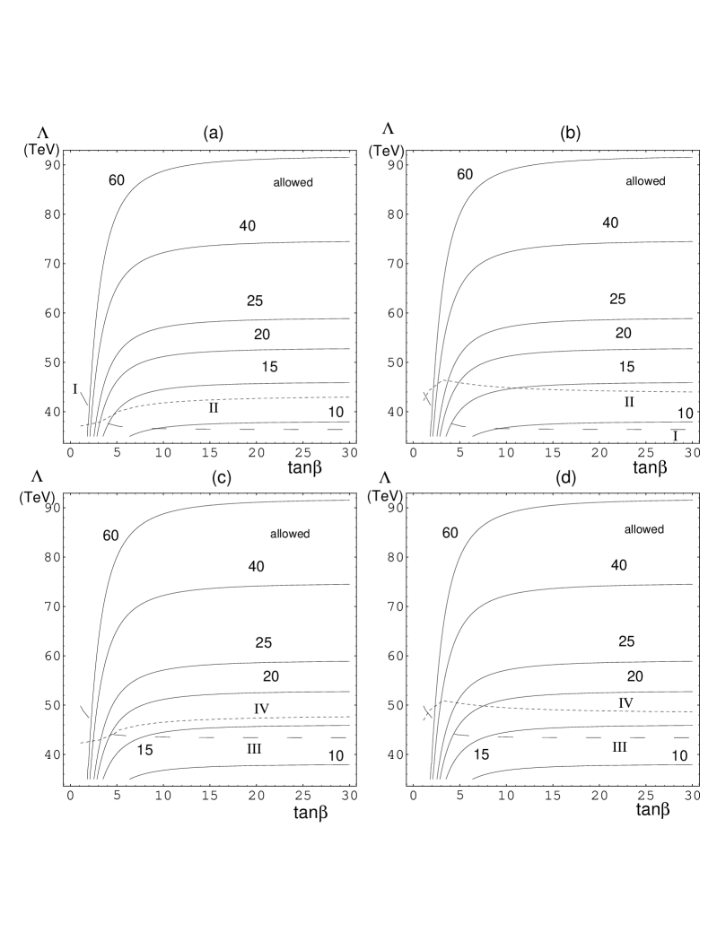
Figure 3.1: Contours of $c(m^{2}_{Z};\mu^{2})=$(10, 15, 20, 25, 40, 60) for a MSSM with a messenger particle content of one $({\bf 5+\bar{5}})$. In Figs.$(a)$ and $(c)$ $sgn(\mu)=-$1 and in Figs.$(b)$ and $(d)$ $sgn(\mu)=+$1. The constraints considered are: (I) $m_{\tilde{e}_{R}}=$75 GeV , (II) $m_{{\tilde{\chi}}^{0}_{1}}+m_{{\tilde{\chi}}^{0}_{2}}=$ 160 GeV, (III) $m_{\tilde{e}_{R}}=$85 GeV, and (IV) $m_{{\tilde{\chi}}^{0}_{1}}+m_{{\tilde{\chi}}^{0}_{2}}=$ 180 GeV. A central value of $m_{top}=$175 GeV is assumed.

We note that $c(m^{2}_{Z},\mu^{2})$ is large throughout most of the parameter space, except for the region where $\tan\beta\;\raisebox{-1.72218pt}{\hbox to0.0pt{$\sim$\hss}}\raisebox{1.72218pt}{$>$}\;$5 and the messenger scale is low. A strong constraint on a lower limit for $\Lambda_{mess}$ comes from the right-handed selectron mass. Contours $m_{\tilde{e}_{R}}=$ 75 GeV ($\sim$ the LEP limit from the run at $\sqrt{s}\approx 170$ GeV [62]) and 85 GeV ($\sim$ the ultimate LEP2 limit [63]) are also plotted. The (approximate) limit on the neutralino masses from the LEP run at $\sqrt{s}\approx 170$ GeV, $m_{\chi^{0}_{1}}+m_{\chi^{0}_{2}}=160$ GeV and the ultimate LEP2 limit, $m_{\chi^{0}_{1}}+m_{\chi^{0}_{2}}\sim 180$ GeV are also shown in Figs.3.1a and 3.1c for $sgn(\mu)=-1$ and Figs.3.1b and 3.1d for $sgn(\mu)=+1$. The constraints from the present and the ultimate LEP2 limits on the chargino mass are weaker than or comparable to those from the selectron and the neutralino masses and are therefore not shown. If $m_{Z}$ were much larger, then $c\sim$ 1. For example, with $m_{Z}=$ 275 GeV (550 GeV) and $\Lambda_{mess}$= 50 (100) TeV, $c(m^{2}_{Z};\mu^{2})$ varies between 1 and 5 for $1.4\;\raisebox{-1.72218pt}{\hbox to0.0pt{$\sim$\hss}}\raisebox{1.72218pt}{$<$}\;\tan\beta\;\raisebox{-1.72218pt}{\hbox to0.0pt{$\sim$\hss}}\raisebox{1.72218pt}{$<$}\;2$, and is $\approx 1$ for $\tan\beta>2$. This suggests that the interpretation that a large value for $c(m^{2}_{Z};\mu^{2})$ implies that $m_{Z}$ is fine tuned is probably correct.

From Fig.3.1 we conclude that in the minimal LEGM model a fine tuning of approximately $7\%$ in the Higgs potential is required to produce the correct value for $m_{Z}$. Further, for this fine tuning the parameters of the model are restricted to the region $\tan\beta\;\raisebox{-1.72218pt}{\hbox to0.0pt{$\sim$\hss}}\raisebox{1.72218pt}{$>$}$ 5 and $\Lambda_{mess}\approx$ 45 TeV, corresponding to $m_{\tilde{e}_{R}}\approx$ 85 GeV. We have also checked that adding more complete $({\bf 5+\bar{5}})$’s does not reduce the fine tuning.

3.3 A Toy Model to Reduce Fine Tuning

3.3.1 Model

In this section the particle content and couplings in the messenger sector that are suffucient to reduce $|m_{H_{u}}^{2}|$ is discussed. The aim is to reduce $m_{\tilde{Q}_{3}}^{2}/m_{H_{u}}^{2}$ at the scale $\Lambda_{mess}$.

The idea is to increase the number of messenger leptons ($SU(2)$ doublets) relative to the number of messenger quarks ($SU(3)$ triplets). This reduces both $m_{\tilde{Q}_{3}}^{2}/m_{H_{u}}^{2}$ and $m_{\tilde{Q}_{3}}^{2}/m^{2}_{\tilde{e}_{R}}$ at the scale $\Lambda_{mess}$ (see Eqn.(3.4)). This leads to a smaller value of $|m_{H_{u}}^{2}|$ in the RG scaling (see Eqn.(3.13)) and the scale $\Lambda_{mess}$ can be lowered since $m_{\tilde{e}_{R}}$ is larger. For example, with three doublets and one triplet at a scale $\Lambda_{mess}=30$ TeV, so that $m_{\tilde{e}_{R}}\approx 85$ GeV, we find $|m_{H_{u}}^{2}(m_{\tilde{Q}_{3}})|\approx(100\hbox{GeV})^{2}$ for $\lambda_{t}=1$. This may be achieved by the following superpotential in the messenger sector

$$W = \lambda_{q_{1}}Sq_{1}\bar{q_{1}}+\lambda_{l_{1}}Sl_{1}\bar{l_{1}}+\lambda_{l_{2}}Sl_{2}\bar{l_{2}}+\lambda_{l_{3}}Sl_{3}\bar{l_{3}}+\frac{1}{3}\lambda_{S}S^{3}$$ (3.15)

$$+\lambda_{\Phi}S\Phi_{-}\Phi_{+}+\frac{1}{3}\lambda_{N}N^{3}+\lambda_{q_{2}}Nq_{2}\bar{q_{2}}+\lambda_{q_{3}}Nq_{3}\bar{q_{3}},$$

where $N$ is a gauge singlet. The two pairs of triplets $q_{2},\bar{q}_{2}$ and $q_{3},\bar{q}_{3}$ are required at low energies to maintain gauge coupling unification. In this model the additional leptons $l_{2},\bar{l}_{2}$ and $l_{3},\bar{l}_{3}$ couple to the singlet $S$, whereas the additional quarks couple to a different singlet $N$ that does not couple to the messenger fields $\Phi_{+}$, $\Phi_{-}$. This can be enforced by discrete symmetries (we discuss such a model in section 3.6). Further, we assume the discrete charges also forbid any couplings between $N$ and $S$ at the renormalizable level (this is true of the model in section 3.6) so that SUSY breaking is communicated first to $S$ and to $N$ only at a higher loop level.

3.3.2 Mass Spectrum

Before quantifying the fine tuning in this model, the mass spectrum of the additional states is briefly discussed. While these fields form complete representations of $SU(5)$, they are not degenerate in mass. The vev and $F$-component of the singlet $S$ gives a mass $\Lambda_{mess}$ to the messenger lepton multiplets if the $F$-term splitting between the scalars is neglected. As the squarks in $q_{i}+\bar{q_{i}}$ ($i$=2,3) do not couple to $S$, they acquire a soft scalar mass from the same two loop diagrams that are responsible for the masses of the MSSM squarks, yielding $m_{\tilde{q}}\approx\alpha_{3}(\Lambda_{mess})\;\Lambda_{SUSY}/(\sqrt{6}\pi)$. The fermions in $q+\bar{q}$ also acquire mass at this scale since, if either $\lambda_{q_{2}}$ or $\lambda_{q_{3}}\sim\;O(1)$, a negative value for $m^{2}_{N}$ (the soft scalar (mass)² of $N$) is generated from the $\lambda_{q}Nq\bar{q}$ coupling at one loop and thus a vev for $N\sim$ $m_{\tilde{q}}$ is generated. The result is $m_{l}/m_{q}\approx\sqrt{6}\pi/\alpha_{3}(\Lambda_{mess})(\Lambda_{mess}/\Lambda_{SUSY})\approx 85$.

The mass splitting in the extra fields introduces a threshold correction to $\sin^{2}\theta_{W}$ if it is assumed that the gauge couplings unify at some high scale $M_{GUT}\approx$10¹⁶ GeV. We estimate that the splitting shifts the prediction for $\sin^{2}\theta_{W}$ by an amount $\approx-$7$\times$ 10${}^{-4}\ln(m_{l}/m_{q})n$, where $n$ is the number of split $({\bf 5+\bar{5}})$. In this case $n=$2 and $m_{l}/m_{q}\sim$ 85, so $\delta$$\sin^{2}\theta_{W}\sim-6\times 10^{-3}$. If $\alpha_{3}(M_{Z})$ and $\alpha_{em}(M_{Z})$ are used as input, then using the two loop RG equations $\sin^{2}\theta_{W}(\overline{MS})=0.233\;\pm\;O(10^{-3})$ is predicted in a minimal SUSY-GUT [8]. The error is a combination of weak scale SUSY and GUT threshold corrections [8]. The central value of the theoretical prediction is a few percent higher than the measured value of $\sin^{2}\theta_{W}(\overline{MS})=0.231\pm 0.0003$ [4]. The split extra fields shift the prediction of $\sin^{2}\theta_{W}$ to $\sim 0.227\pm\;O(10^{-3})$ which is a few percent lower than the experimental value. In sections 3.5 and 3.6 we show that this spectrum is derivable from a $SU(5)\times SU(5)$ GUT in which the GUT threshold corrections to $\sin^{2}\theta_{W}$ could be $\sim O(10^{-3})-O(10^{-2})$ [64]. It is possible that the combination of these GUT threshold corrections and the split extra field threshold corrections make the prediction of $\sin^{2}\theta_{W}$ more consistent with the observed value.

3.3.3 Fine Tuning

To quantify the fine tuning in these class of models the analysis of section 3.2 is applied. In our RG analysis the RG scaling of $\lambda_{t}$, the effect of the extra vector-like triplets on the RG scaling of the gauge couplings, and weak scale SUSY threshold corrections were neglected. We have checked a posteriori that this approximation is consistent. As in section 3.2, the two free parameters are chosen to be $\Lambda_{mess}$ and $\tan\beta$. Contours of constant $c(m^{2}_{Z},\mu^{2})$ are presented in Fig.3.2.

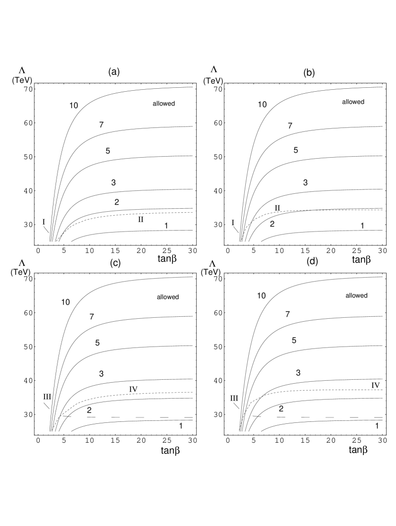
Figure 3.2: Contours of $c(m^{2}_{Z};\mu^{2})=$(1, 2, 3, 5, 7, 10) for a MSSM with a messenger particle content of three $(l+\bar{l})$’s and one $(q+\bar{q})$. In Figs.$(a)$ and $(c)$ $sgn(\mu)=-$1 and in Figs.$(b)$ and $(d)$ $sgn(\mu)=+$1. The constraints considered are: (I) $m_{\tilde{e}_{R}}=$75 GeV , (II) $m_{{\tilde{\chi}}^{0}_{1}}+m_{{\tilde{\chi}}^{0}_{2}}=$ 160 GeV, (III) $m_{\tilde{e}_{R}}=$85 GeV, and (IV) $m_{{\tilde{\chi}}^{0}_{1}}+m_{{\tilde{\chi}}^{0}_{2}}=$ 180 GeV. A central value of $m_{top}=$175 GeV is assumed.

We show contours of $m_{\chi^{0}_{1}}+m_{\chi^{0}_{2}}=160$ GeV, and $m_{\tilde{e}_{R}}=75$ GeV in Fig. 3.2a for $sgn(\mu)=-1$ and in Fig.3.2b for $sgn(\mu)=+1$. These are roughly the limits from the LEP run at $\sqrt{s}\approx 170$ GeV [62]). The (approximate) ultimate LEP2 reaches [63]: $m_{\chi^{0}_{1}}+m_{\chi^{0}_{2}}=180$ GeV and $m_{\tilde{e}_{R}}=85$ GeV are shown in Fig.3.2c for $sgn(\mu)=-1$ and Fig.3.2d for $sgn(\mu)=+1$. Since $\mu^{2}(\approx$ (100 GeV)${}^{2})$ is much smaller in these models than in the minimal LEGM model, the neutralinos ($\chi^{0}_{1}\;\hbox{and}\;\chi^{0}_{2}$) are lighter so that the neutralino masses provide a stronger constraint on $\Lambda_{mess}$ than does the slepton mass limit. The chargino constraints are comparable to the neutralino constraints and are thus not shown. It is clear that there are areas of parameter space in which the fine tuning is improved to $\sim$ 40$\%$ (see Fig.3.2).

While this model improves the fine tuning required of the $\mu$ parameter, it would be unsatisfactory if further fine tunings were required in other sectors of the model, for example, the sensitivity of $m^{2}_{Z}$ to $\mu^{2}_{3}$, $\Lambda_{mess}$ and $\lambda_{t}$ and the sensitivity of $m_{t}$ to $\mu^{2}$, $\mu^{2}_{3}$, $\Lambda_{mess}$ and $\lambda_{t}$. We have checked that all these are less than or comparable to $c(m^{2}_{Z};\mu^{2})$. We now discuss the other fine tunings in detail.

For large $\tan\beta$, the sensitivity of $m^{2}_{Z}$ to $\mu_{3}^{2}$, $c(m^{2}_{Z};\mu^{2}_{3})$ $\propto$ $1/\tan^{2}\beta$, and is therefore smaller than $c(m^{2}_{Z};\mu^{2})$. Our numerical analysis shows that for all $\tan\beta$ $c(m^{2}_{Z};\mu^{2}_{3})\;\raisebox{-1.72218pt}{\hbox to0.0pt{$\sim$\hss}}\raisebox{1.72218pt}{$<$}\;c(m^{2}_{Z};\mu^{2})$.

In the one loop approximation $m^{2}_{H_{u}}$ and $m^{2}_{H_{d}}$ at the weak scale are proportional to $\Lambda^{2}_{mess}$ since all the soft masses scale with $\Lambda_{mess}$ and there is only a weak logarithmic dependence on $\Lambda_{mess}$ through the gauge couplings. We have checked numerically that $(\Lambda_{mess}^{2}/m^{2}_{H_{u}})(\partial m^{2}_{H_{u}}/\partial\Lambda_{mess}^{2})\sim 1$. Then, $c(m_{Z}^{2};\Lambda_{mess}^{2})\approx c(m_{Z}^{2};m^{2}_{H_{d}})+c(m_{Z}^{2};m^{2}_{H_{u}})$. We find that $c(m_{Z}^{2};\Lambda_{mess}^{2})\approx c(m_{Z}^{2};\mu^{2})+$1 over most of the parameter space.

In the one loop approximation, $m^{2}_{H_{u}}(t)$ is

$$m^{2}_{H_{u}}(t)\approx m^{2}_{H_{u},0}+(m^{2}_{\tilde{Q}_{3},0}+m^{2}_{\tilde{u}^{c}_{3},0}+m^{2}_{H_{u},0})(e^{-\frac{3\lambda^{2}_{t}}{8\pi^{2}}t}-1).$$ (3.16)

Then, using $t\approx\ln(\Lambda_{mess}/m_{\tilde{Q}_{3}})\approx\ln(\sqrt{6}\pi/\alpha_{3})\approx$ 4.5 and $\lambda_{t}\approx$ 1, $c(m^{2}_{Z};\lambda_{t})$ is (see appendix)

$$c(m^{2}_{Z};\lambda_{t})\approx\frac{4}{m^{2}_{Z}}\frac{\partial m^{2}_{H_{u}}(t)}{\partial\lambda^{2}_{t}}\approx 50\frac{m^{2}_{\tilde{Q}_{3}}}{(\hbox{600 GeV})^{2}}.$$ (3.17)

This result measures the sensitivity of $m^{2}_{Z}$ to the value of $\lambda_{t}$ at the electroweak scale. While this sensitivity is large, it does not reflect the fact that $\lambda_{t}(M_{Pl})$ is the fundamental parameter of the theory, rather than $\lambda_{t}(m_{weak})$. We find by both numerical and analytic computations that, for this model with three $({\bf 5+\bar{5}})$’s in addition to the MSSM particle content, $\delta\lambda_{t}(m_{weak})\approx 0.1\times\delta\lambda_{t}(M_{Pl})$, and therefore

$$c(m^{2}_{Z};\lambda_{t}(M_{Pl}))\approx 5\frac{m^{2}_{\tilde{Q}_{3}}}{(\hbox{600 GeV})^{2}}.$$ (3.18)

For a scale of $\Lambda_{mess}$ = 50 TeV ($m_{\tilde{Q}_{3}}\approx$ 600 GeV), $c(m^{2}_{Z};\lambda_{t}(M_{Pl}))$ is comparable to $c(m^{2}_{Z};\mu^{2})$ which is $\approx$ 4 to 5. At a lower messenger scale, $\Lambda_{mess}\approx$ 35 TeV, corresponding to squark masses of $\approx$ 450 GeV, the sensitivity of $m^{2}_{Z}$ to $\lambda_{t}(M_{Pl})$ is $\approx$ 2.8. This is comparable to $c(m^{2}_{Z};\mu^{2})$ evaluated at the same scale.

We now discuss the sensitivity of $m_{t}$ to the fundamental parameters. Since, $m_{t}^{2}=\frac{1}{2}v^{2}\sin^{2}\beta\lambda_{t}^{2}$, we get

$$c(m_{t};\lambda_{i})=\delta_{\lambda_{t}\lambda_{i}}+\frac{1}{2}c(m_{Z}^{2};\lambda_{i})+\frac{\cos^{3}\beta}{\sin\beta}\frac{\partial\tan\beta}{\partial\lambda_{i}}\lambda_{i}.$$ (3.19)

Numerically we find that the last term in $c(m_{t};\lambda_{i})$ is small compared to $c(m_{Z}^{2};\lambda_{i})$ and thus over most of parameter space $c(m_{t};\lambda_{i})\approx\frac{1}{2}c(m_{Z}^{2};\lambda_{i})$. As before, the sensitivity of $m_{t}$ to the value of $\lambda_{t}$ at the GUT/Planck scale is much smaller than the sensitivity to the value of $\lambda_{t}$ at the weak scale.

3.3.4 Sparticle Spectrum

The sparticle spectrum is now briefly discussed to highlight deviations from the mass relations predicted in the minimal LEGM model. For example, with three doublets and one triplet at a scale of $\Lambda=$ 50 TeV, the soft scalar masses (in GeV) at a renormalization scale $\mu^{2}_{RG}=m^{2}_{t}+\frac{1}{2}(m^{2}_{\tilde{Q}_{3}}+m^{2}_{\tilde{u}^{c}_{3}})$ $\approx($630 GeV$)^{2}$, for $\lambda_{t}=$ 1, are shown in Table 3.1.

$m_{\tilde{Q}_{1,2}}$	$m_{\tilde{u}^{c}_{1,2}}$	$m_{\tilde{d}^{c}_{i}}$	$m_{\tilde{L}_{i},H_{d}}$	$m_{\tilde{e}^{c}_{i}}$
687	616	612	319	125

$m_{\tilde{Q}_{3}}$	$m_{\tilde{u}^{c}_{3}}$
656	546

Table 3.1: Soft scalar masses in GeV for messenger particle content of three $(l+\bar{l})$’s and one $q+\bar{q}$ and a scale $\Lambda_{mess}=50$ TeV.

Two observations that are generic to this type of model are: (i) By construction, the spread in the soft scalar masses is less than in the minimal LEGM model. (ii) The gaugino masses do not satisfy the one loop SUSY-GUT relation $M_{i}/\alpha_{i}$ = constant. In this case, for example, $M_{3}/\alpha_{3}:M_{2}/\alpha_{2}\approx$ 1$:$3 and $M_{3}/\alpha_{3}:M_{1}/\alpha_{1}\approx$ 5$:$11 to one loop.

We have also found that for $\tan\beta$ $\sim$$>$ 3, the Next Lightest Supersymmetric Particle (NLSP) is one of the neutralinos, whereas for $\tan\beta$ $\sim$$<$ 3, the NLSP is the right-handed stau. Further, for these small values of $\tan\beta$, the three right-handed sleptons are degenerate within $\approx$ 200 MeV.

3.4 NMSSM

In section 3.2, the $\mu$ term and the SUSY breaking mass $\mu^{2}_{3}$ were put in by hand. There it was found that these parameters had to be fine tuned in order to correctly reproduce the observed $Z$ mass. The extent to which this is a “problem” may only be evaluated within a specific model that generates both the $\mu$ and $\mu^{2}_{3}$ terms.

For this reason, in this section a possible way to generate both the $\mu$ term and $\mu^{2}_{3}$ term in a manner that requires a minimal modification to the model of either section 3.1 or section 3.3 is discussed. The easiest way to generate these mass terms is to introduce a singlet $N$ and add the interaction $NH_{u}H_{d}$ to the superpotential (the NMSSM) [56]. The vev of the scalar component of $N$ generates $\mu$ and the vev of the $F$-component of $N$ generates $\mu_{3}^{2}$.

We note that for the “toy model” solution to the fine tuning problem (section 3.3), the introduction of the singlet occurs at no additional cost. Recall that in that model it was necessary to introduce a singlet $N$, distinct from $S$, such that the vev of $N$ gives mass to the extra light vector-like triplets, $q_{i},\bar{q}_{i}\;(i=2,3)$ (see Eqn.(3.15)). Further, discrete symmetries (see section 3.6) are imposed to isolate $N$ from SUSY breaking in the messenger sector. This last requirement is necessary to solve the fine tuning problem: if both the scalar and $F$-component of $N$ acquired a vev at the same scale as $S$, then the extra triplets that couple to $N$ would also act as messenger fields. In this case the messenger fields would form complete $({\bf 5+\bar{5}})$’s and the fine tuning problem would be reintroduced. With $N$ isolated from the messenger sector at tree level, a vev for $N$ at the electroweak scale is naturally generated, as discussed in section 3.3.

We also comment on the necessity and origin of these extra triplets. Recall that in the toy model of section 3.3 these triplets were required to maintain the SUSY-GUT prediction for $\sin^{2}\theta_{W}$. Further, we shall also see that they are required in order to generate a large enough $-m^{2}_{N}$ (the soft scalar (mass)² of the singlet $N$). Finally, in the GUT model of section 3.6, the lightness of these triplets (as compared to the missing doublets) is the consequence of a doublet-triplet splitting mechanism.

The superpotential in the electroweak symmetry breaking sector is

$$W=\frac{\lambda_{N}}{3}N^{3}+\lambda_{q}Nq\bar{q}-\lambda_{H}NH_{u}H_{d},$$ (3.20)

which is similar to an NMSSM except for the coupling of $N$ to the triplets. The superpotential in the messenger sector is given by Eqn.(3.15).

The scalar potential is

$$V = \sum_{i}|F_{i}|^{2}+m_{N}^{2}|N|^{2}+m_{H_{u}}^{2}|H_{u}|^{2}+m_{H_{d}}^{2}|H_{d}|^{2}+\hbox{D-terms}$$ (3.21)

$$-(A_{H}NH_{u}H_{d}+h.c.)+V_{1-loop}.$$

The extremization conditions for the vevs of the real components of $N$, $H_{u}$ and $H_{d}$, denoted by $v_{N}$, $v_{u}$ and $v_{d}$ respectively (with $v=\sqrt{v_{u}^{2}+v_{d}^{2}}\approx 250$ GeV), are

$$v_{N}(\tilde{m}^{2}_{N}+\lambda^{2}_{H}\frac{v^{2}}{2}+\lambda^{2}_{N}v^{2}_{N}-\lambda_{H}\lambda_{N}v_{u}v_{d})-\frac{1}{\sqrt{2}}A_{H}v_{u}v_{d}=0,$$ (3.22)

$$\frac{1}{2}m_{Z}^{2} = \frac{\tilde{\mu}_{1}^{2}-\tilde{\mu}_{2}^{2}\tan^{2}\beta}{\tan^{2}\beta-1},$$ (3.23)

$$\sin 2\beta = 2\frac{\mu^{2}_{3}}{\tilde{\mu}_{2}^{2}+\tilde{\mu}_{1}^{2}},$$ (3.24)

with

$$\mu^{2} = \frac{1}{2}\lambda_{H}^{2}v_{N}^{2},$$ (3.25)

$$\mu_{3}^{2} = -\frac{1}{2}\lambda_{H}^{2}v_{u}v_{d}+\frac{1}{2}\lambda_{H}\lambda_{N}v_{N}^{2}+A_{H}\frac{1}{\sqrt{2}}v_{N},$$ (3.26)

$$\tilde{m}^{2}_{i} = m^{2}_{i}+2\frac{\partial V_{1-loop}}{\partial v^{2}_{i}}\hbox{};\;\;i=(u,d,N).$$ (3.27)

We now comment on the expected size of the Yukawa couplings $\lambda_{q}$, $\lambda_{N}$ and $\lambda_{H}$. We must use the RGE’s to evolve these couplings from their values at $M_{GUT}$ or $M_{Pl}$ to the weak scale. The quarks and the Higgs doublets receive wavefunction renormalization from $SU(3)$ and $SU(2)$ gauge interactions respectively, whereas the singlet $N$ does not receive any wavefunction renormalization from gauge interactions at one loop. So, the couplings at the weak scale are in the order: $\lambda_{q}\sim O(1)>\lambda_{H}>\lambda_{N}$ if they all are $O(1)$ at the GUT/Planck scale.

We remark that without the $Nq\bar{q}$ coupling, it is difficult to drive a vev for $N$ as we now show below. The one loop RGE for $m_{N}^{2}$ is

$$\frac{dm_{N}^{2}}{dt}\approx\frac{6\lambda_{N}^{2}}{8\pi^{2}}m_{N}^{2}(t)+\frac{2\lambda_{H}^{2}}{8\pi^{2}}(m_{H_{u}}^{2}(t)+m_{H_{d}}^{2}(t)+m_{N}^{2}(t))+\frac{3\lambda_{q}^{2}}{8\pi^{2}}(m_{\tilde{q}}^{2}(t)+m_{\tilde{\bar{q}}}^{2}(t)).$$ (3.28)

Since $N$ is a gauge-singlet, $m_{N}^{2}=0$ at $\Lambda_{mess}$. Further, if $\lambda_{q}=0$, an estimate for $m_{N}^{2}$ at the weak scale is then

$$m_{N}^{2}\approx-\frac{2\lambda^{2}_{H}}{8\pi^{2}}(m_{H_{u},0}^{2}+m_{H_{d},0}^{2})\ln\left(\frac{\Lambda_{mess}}{m_{H_{d}}}\right),$$ (3.29)

i.e., $\lambda_{H}$ drives $m_{N}^{2}$ negative. The extremization condition for $v_{N}$, Eqn.(3.22), and using Eqns.(3.24) and (3.26) (neglecting $A_{H}$) shows that

$$m^{2}_{N}+\lambda^{2}_{H}\frac{v^{2}}{2}\approx\lambda^{2}_{H}\left(\frac{v^{2}}{2}-\frac{2}{8\pi^{2}}(m_{H_{u},0}^{2}+m_{H_{d},0}^{2})\ln\left(\frac{\Lambda_{mess}}{m_{H_{d}}}\right)\right)$$ (3.30)

has to be negative for $N$ to acquire a vev. This implies that $m_{H_{u}}^{2}$ and $m_{H_{d}}^{2}$ at $\Lambda_{mess}$ have to be greater than $\sim(350\;\hbox{GeV})^{2}$ which implies that a fine tuning of a few percent is required in the electroweak symmetry breaking sector. With $\lambda_{q}\sim O(1)$, however, there is an additional negative contribution to $m_{N}^{2}$ given approximately by

$$-\frac{3\lambda^{2}_{q}}{8\pi^{2}}(m_{\tilde{q},0})^{2}+m_{\tilde{\bar{q}},0}^{2})\ln\left(\frac{\Lambda_{mess}}{m_{\tilde{q}}}\right).$$ (3.31)

This contribution dominates the one in Eqn.(3.29) since $\lambda_{q}>\lambda_{H}$ and the squarks $\tilde{q}$, $\tilde{\bar{q}}$ have soft masses larger than the Higgs. Thus, with $\lambda_{q}\neq 0$, $m^{2}_{N}+\lambda^{2}_{H}v^{2}/2$ is naturally negative.

Fixing $m_{Z}$ and $m_{t}$, we have the following parameters : $\Lambda_{mess}$, $\lambda_{q}$, $\lambda_{H}$, $\lambda_{N}$, $\tan\beta$, and $v_{N}$. Three of the parameters are fixed by the three extremization conditions, leaving three free parameters that for convenience are chosen to be $\Lambda_{mess}$, $\tan\beta\geq$0, and $\lambda_{H}$. The signs of the vevs are fixed to be positive by requiring a stable vacuum and no spontaneous CP violation. The three extremization equations determine the following relations

$$\lambda_{N} = \frac{2}{\lambda_{H}v^{2}_{N}}(\mu^{2}_{3}+\frac{1}{4}\lambda^{2}_{H}\sin 2\beta v^{2}-\frac{1}{\sqrt{2}}A_{H}v_{N}),$$ (3.32)

$$v_{N} = \sqrt{2}\frac{\mu}{\lambda_{H}},$$ (3.33)

$$\tilde{m}^{2}_{N} = \lambda_{N}\lambda_{H}\frac{1}{2}\sin 2\beta v^{2}-\lambda^{2}_{N}v^{2}_{N}-\frac{1}{2}\lambda^{2}_{H}v^{2}+\frac{1}{2\sqrt{2}}A_{H}\sin 2\beta\frac{v^{2}}{v_{N}},$$ (3.34)

where

$$\mu^{2} = -\frac{1}{2}m^{2}_{Z}+\frac{\tilde{m}_{H_{u}}^{2}\tan^{2}\beta-\tilde{m}^{2}_{H_{d}}}{1-\tan^{2}\beta},$$ (3.35)

$$2\mu^{2}_{3} = \sin 2\beta(2\mu^{2}+\tilde{m}_{H_{u}}^{2}+\tilde{m}^{2}_{H_{d}}).$$ (3.36)

The superpotential term $NH_{u}H_{d}$ couples the RGE’s for $m^{2}_{H_{u}}$, $m^{2}_{H_{d}}$ and $m^{2}_{N}$. Thus the values of these masses at the electroweak scale are, in general, complicated functions of the Yukawa parameters $\lambda_{t}$, $\lambda_{H}$, $\lambda_{N}$ and $\lambda_{q}$. In our case, two of these Yukawa parameters ($\lambda_{q}$ and $\lambda_{N}$) are determined by the extremization equations and a closed form expression for the derived quantities cannot be found. To simplify the analysis, we neglect the dependence of $m^{2}_{H_{u}}$ and $m^{2}_{H_{d}}$ on $\lambda_{H}$ induced in RG scaling from $\Lambda_{mess}$ to the weak scale. Then $m_{H_{u}}^{2}$ and $m_{H_{d}}^{2}$ depend only on $\Lambda_{mess}$ and $\tan\beta$ and thus closed form solutions for $\lambda_{N}$, $v_{N}$ and $\tilde{m}^{2}_{N}$ can be obtained using the above equations. Once $\tilde{m}_{N}^{2}$ at the weak scale is obtained, the value of $\lambda_{q}$ is obtained by using an approximate analytic solution. An exact numerical solution of the RGE’s then shows that the above approximation is consistent.

3.4.1 Fine Tuning and Phenomenology

The fine tuning functions we consider below are $c(O;\lambda_{H})$, $c(O;\lambda_{N})$, $c(O;\lambda_{t})$, $c(O;\lambda_{q})$ and $c(O;\Lambda_{mess})$ where $O$ is either $m^{2}_{Z}$ or $m_{t}$. The expressions for the fine tuning functions and other details are given in the appendix. In our RG analysis the approximations discussed in subsection 3.3.3 and above were used and found to be consistent. Fine tuning contours of $c(m^{2}_{Z};\lambda_{H})$ are displayed in Figs.3.3a and Fig.3.3b for $\lambda_{H}=0.1$ and Figs.3.3c and 3.3d for $\lambda_{H}=0.5$. We have found by numerical computations that the other fine tuning functions are either smaller or comparable to $c(m^{2}_{Z};\lambda_{H})$.

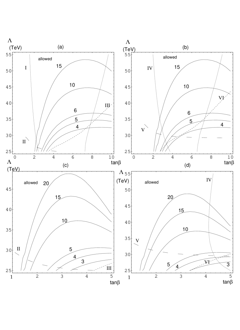
Figure 3.3: Contours of $c(m^{2}_{Z};\lambda_{H})$ for the NMSSM of section 3.4 and a messenger particle content of three $(l+\bar{l})$’s and one $(q+\bar{q})$. In Figs.$(a)$ and $(b)$, $c(m^{2}_{Z};\lambda_{H})$=(4, 5, 6, 10, 15) and $\lambda_{H}=$0.1. In Figs.$(c)$ and $(d)$, $c(m^{2}_{Z};\lambda_{H})=$(3, 4, 5, 10, 15, 20) and $\lambda_{H}$=0.5. The constraints considered are: 5(I) $m_{h}+m_{a}=m_{Z}$, (II) $m_{\tilde{e}_{R}}=$75 GeV, (III) $m_{{\tilde{\chi}}^{0}_{1}}+m_{{\tilde{\chi}}^{0}_{2}}=$ 160 GeV, (IV) $m_{h}=$ 92 GeV, (V) $m_{\tilde{e}_{R}}=$85 GeV, and (VI) $m_{{\tilde{\chi}}^{0}_{1}}+m_{{\tilde{\chi}}^{0}_{2}}=$ 180 GeV. For $\lambda_{H}=$0.5, the limit $m_{h}\stackrel{{\scriptstyle>}}{{\sim}}$ 70 GeV constrains $\tan\beta\stackrel{{\scriptstyle<}}{{\sim}}$ 5 (independent of $\Lambda_{mess}$) and is thus not shown. A central value of $m_{top}=$175 GeV is assumed.

We now discuss the existing phenomenological constraints on our model and also the ultimate constraints if LEP2 does not discover SUSY/light Higgs($h$). These are shown in Figs.3.3a, 3.3c and Figs.3.3b, 3.3d respectively. We consider the processes $e^{+}e^{-}\rightarrow Zh$, $e^{+}e^{-}$$\rightarrow(h+\hbox{pseudoscalar})$, $e^{+}e^{-}$$\rightarrow$ $\chi^{+}\chi^{-}$, $e^{+}e^{-}$$\rightarrow$ $\chi^{0}_{1}\chi^{0}_{2}$, and $e^{+}e^{-}$$\rightarrow$ $\tilde{e}_{R}\tilde{e}^{*}_{R}$ observable at LEP. Since this model also has a light pseudoscalar, we also consider upsilon decays $\Upsilon$$\rightarrow(\gamma+\hbox{pseudoscalar})$. We find that the model is phenomenologically viable and requires a $\sim$ 20$\%$ tuning even if no new particles are discovered at LEP2.

We begin with the constraints on the scalar and pseudoscalar spectra of this model. There are three neutral scalars, two neutral pseudoscalars and one complex charged scalar. We first consider the mass spectrum of the pseudoscalars. At the boundary scale $\Lambda_{mess}$, SUSY is softly broken in the visible sector only by the soft scalar masses and the gaugino masses. Further, the superpotential of Eqn.(3.20) has an $R$-symmetry. Therefore, at the tree level, i.e., with $A_{H}=$0, the scalar potential of the visible sector (Eqn.(3.21)) has a global symmetry. This symmetry is spontaneously broken by the vevs of $N^{R}$, $H^{R}_{u}$, and $H^{R}_{d}$ (the superscript $R$ denotes the real component of fields), so that one physical pseudoscalar is massless at tree level. It is

$$a=\frac{1}{\sqrt{v^{2}_{N}+v^{2}\sin^{2}2\beta}}\left(v_{N}N^{I}+v\sin 2\beta\cos\beta H_{u}^{I}+v\sin 2\beta\sin\beta H_{d}^{I}\right),$$ (3.37)

where the superscripts $I$ denote the imaginary components of the fields. The second pseudoscalar,

$$A\sim-\frac{2}{v_{N}}N^{I}+\frac{H_{u}^{I}}{v\sin\beta}+\frac{H_{d}^{I}}{v\cos\beta},$$ (3.38)

acquires a mass

$$m^{2}_{A}=\frac{1}{2}\lambda_{H}\lambda_{N}v^{2}_{N}(\tan\beta+\cot\beta)+\lambda_{H}\lambda_{N}v^{2}\sin 2\beta$$ (3.39)

through the $|F_{N}|^{2}$ term in the scalar potential.

The pseudoscalar $a$ acquires a mass once an $A_{H}$-term is generated, at one loop, through interactions with the gauginos. Including only the wino contribution in the one loop RGE, $A_{H}$ is given by

$$A_{H} \approx 6\frac{\alpha_{2}(\Lambda_{mess})}{4\pi}M_{2}\lambda_{H}\ln\left(\frac{\Lambda_{mess}}{M_{2}}\right),$$ (3.40)

$$\approx 20\;\lambda_{H}\left(\frac{M_{2}}{280\hbox{GeV}}\right)\hbox{GeV},$$

where $M_{2}$ is the wino mass at the weak scale. Neglecting the mass mixing between the two pseudoscalars, the mass of the pseudo-Nambu-Goldstone boson is computed to be

$$m^{2}_{a} = \frac{9}{\sqrt{2}}Av_{N}v_{u}v_{d}/(v_{N}^{2}+v^{2}\sin^{2}2\beta)$$ (3.41)

$$\approx (40)^{2}\left(\frac{\lambda_{H}}{0.1}\right)\frac{M_{2}}{280\hbox{GeV}}\sin 2\beta\left(\frac{\frac{{\textstyle v_{N}}}{{\textstyle 250}\hbox{GeV}}}{\sin^{2}2\beta+\left(\frac{{\textstyle v_{N}}}{{\textstyle 250}\hbox{GeV}}\right)^{2}}\right)(\hbox{GeV})^{2}.$$

If the mass of $a$ is less than 7.2 GeV, it could be detected in the decay $\Upsilon\rightarrow a+\gamma$ [4]. Comparing the ratio of decay width for $\Upsilon\rightarrow a+\gamma$ to $\Upsilon\rightarrow\mu^{-}+\mu^{+}$ [4, 65], the limit

$$\frac{\sin 2\beta\tan\beta}{\sqrt{(\frac{{\textstyle v_{N}}}{{\textstyle 250}\hbox{GeV}})^{2}+\sin^{2}2\beta}}<0.43$$ (3.42)

is found.

Further constraints on the spectra are obtained from collider searches. The non-detection of $Z\rightarrow$ scalar + $a$ at LEP implies that the combined mass of the lightest Higgs scalar and $a$ must exceed $\sim$ 92 GeV. Also, the process $e^{+}e^{-}$ $\rightarrow$$Zh$ may be observable at LEP2. For $\lambda_{H}=0.1$, the constraint $m_{h}+m_{a}\;\raisebox{-1.72218pt}{\hbox to0.0pt{$\sim$\hss}}\raisebox{1.72218pt}{$>$}\;92$ GeV is stronger than $m_{h}\;\raisebox{-1.72218pt}{\hbox to0.0pt{$\sim$\hss}}\raisebox{1.72218pt}{$>$}\;70$ GeV which is the limit from LEP at $\sqrt{s}\approx 170$ GeV [62]. The contour of $m_{h}+m_{a}=92$ GeV is shown in Fig.3.3a. In Fig.3.3b, we show the contour of $m_{h}=92$ GeV ($\sim$ the ultimate LEP2 reach [66]). For $\lambda_{H}=0.5$, we find that the constraint $m_{h}\;\raisebox{-1.72218pt}{\hbox to0.0pt{$\sim$\hss}}\raisebox{1.72218pt}{$>$}\;70$ GeV is stronger than $m_{h}+m_{a}\;\raisebox{-1.72218pt}{\hbox to0.0pt{$\sim$\hss}}\raisebox{1.72218pt}{$>$}\;92$ GeV and restricts $\tan\beta\;\raisebox{-1.72218pt}{\hbox to0.0pt{$\sim$\hss}}\raisebox{1.72218pt}{$<$}\;5$ independent of $\Lambda_{mess}$. The contour $m_{h}=92$ GeV is shown in Fig.3.3d. We note that the allowed parameter space is not significantly constrained. We find that these limits make the constraint of Eqn.(3.42) redundant. The left-right mixing between the two top squarks was neglected in computing the top squark radiative corrections to the Higgs masses.

The pseudo-Nambu-Goldstone boson $a$ might be produced along with the lightest scalar $h$ at LEP. The (tree-level) cross section in units of $R=87/s$ nb is

$$\sigma(e^{+}e^{-}\rightarrow h\;a)\approx 0.15\frac{s^{2}}{(s-m_{Z}^{2})^{2}}\;\lambda^{2}\;v\left(1,\frac{m^{2}_{h}}{s},\frac{m^{2}_{a}}{s}\right)^{3},$$ (3.43)

where $g\lambda/\cos\theta_{W}$ is the $Z(a$$\partial$$h-h$$\partial$$a)$ coupling, and
$v(x,y,z)=\sqrt{(x-y-z)^{2}-4yz}$. If $h=c_{N}N^{R}+c_{u}H_{u}^{R}+c_{d}H_{d}^{R}$, then

$$\lambda=\sin 2\beta\frac{\cos\beta\;c_{u}-\sin\beta\;c_{d}}{\sqrt{(\frac{{\textstyle v_{N}}}{{\textstyle 250}\hbox{GeV}})^{2}+\sin^{2}2\beta}}.$$ (3.44)

We have numerically checked the parameter space allowed by $m_{h}\;\raisebox{-1.72218pt}{\hbox to0.0pt{$\sim$\hss}}\raisebox{1.72218pt}{$>$}\;70$ GeV and $\lambda_{H}\leq$0.5 and have found the production cross section for $h\;a$ to be less than both the current limit set by DELPHI [67] and a (possible) exclusion limit of 30 fb [66] at $\sqrt{s}\approx$ 192 GeV. The production cross-section for $h\;A$ is larger than for $h\;a$ and $A$ is therefore in principle easier to detect. However, for the parameter space allowed by $m_{h}\;\raisebox{-1.72218pt}{\hbox to0.0pt{$\sim$\hss}}\raisebox{1.72218pt}{$>$}\;70$ GeV, numerical calculations show that $m_{A}\;\raisebox{-1.72218pt}{\hbox to0.0pt{$\sim$\hss}}\raisebox{1.72218pt}{$>$}\;$ 125 GeV, so that this channel is not kinematically accessible.

The charged Higgs mass is

$$m^{2}_{H^{\pm}}=m^{2}_{W}+m^{2}_{H_{u}}+m^{2}_{H_{d}}+2\mu^{2}$$ (3.45)

which is greater than about 200 GeV in this model since $m_{H_{d}}^{2}\;\raisebox{-1.72218pt}{\hbox to0.0pt{$\sim$\hss}}\raisebox{1.72218pt}{$>$}\;(200\;\hbox{GeV})^{2}$ for $\Lambda_{mess}\;\raisebox{-1.72218pt}{\hbox to0.0pt{$\sim$\hss}}\raisebox{1.72218pt}{$>$}\;35$ TeV and as $\mu^{2}\sim-m^{2}_{H_{u}}$.

The neutralinos and charginos may be observable at LEP2 at $\sqrt{s}\approx 192$ GeV if $m_{\chi^{+}}\;\raisebox{-1.72218pt}{\hbox to0.0pt{$\sim$\hss}}\raisebox{1.72218pt}{$<$}\;95$ GeV and $m_{\chi^{0}_{1}}+m_{\chi^{0}_{2}}\;\raisebox{-1.72218pt}{\hbox to0.0pt{$\sim$\hss}}\raisebox{1.72218pt}{$<$}\;180$ GeV. These two constraints are comparable, and thus only one of these is displayed in Figs.3.3b and 3.3d, for $\lambda_{H}=0.1$ and $\lambda_{H}=0.5$ repectively. Also, contours of $m_{\chi^{0}_{1}}+m_{\chi^{0}_{2}}=$ 160 GeV ($\sim$ the LEP kinematic limit at $\sqrt{s}\approx 170$ GeV) are shown in Figs.3.3a and 3.3c. Contours of 85 GeV ($\sim$ the ultimate LEP2 limit) and 75 GeV ($\sim$ the LEP limit from $\sqrt{s}\approx 170$ GeV) for the right-handed selectron mass further constrain the parameter space.

The results presented in all the figures are for a central value of $m_{t}$=175 GeV. We have varied the top quark mass by 10 GeV about the central value of $m_{t}$= 175 GeV and have found that both the fine tuning measures and the LEP2 constraints (the Higgs mass and the neutralino masses) vary by $\approx$ 30 $\%$, but the qualitative features are unchanged.

We see from Fig.3.3 that there is parameter space allowed by the present limits in which the tuning is $\approx$ 30 $\%$. Even if no new particles are discovered at LEP2, the tuning required for some region is $\approx$ 20$\%$.

It is also interesting to compare the fine tuning measures with those found in the minimal LEGM model (one messenger $({\bf 5+\bar{5}})$) with an extra singlet $N$ to generate the $\mu$ and $\mu^{2}_{3}$ terms. In Fig.3.4 the fine tuning contours for $c(m^{2}_{Z};\lambda_{H})$ are presented for $\lambda_{H}$=0.1.

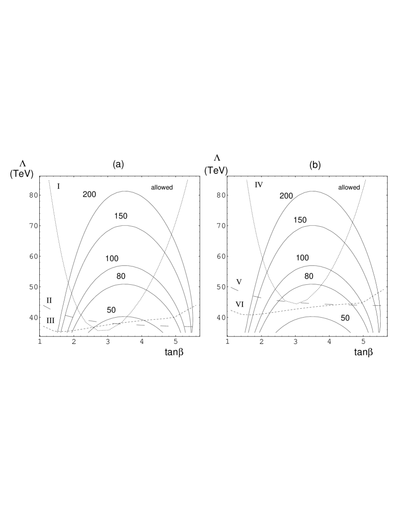
Figure 3.4: Contours of $c(m^{2}_{Z};\lambda_{H})=$(50, 80, 100, 150, 200) for the NMSSM of section 3.4 with $\lambda_{H}=$0.1 and a messenger particle content of one $({\bf 5+\bar{5}})$. The constraints considered are: (I) $m_{h}+m_{a}=m_{Z}$, (II) $m_{\tilde{e}_{R}}=$75 GeV, (III) $m_{{\tilde{\chi}}^{0}_{1}}+m_{{\tilde{\chi}}^{0}_{2}}=$ 160 GeV, (IV) $m_{h}=$92 GeV, (V) $m_{\tilde{e}_{R}}=$85 GeV, and (VI) $m_{{\tilde{\chi}}^{0}_{1}}+m_{{\tilde{\chi}}^{0}_{2}}=$ 180 GeV. A central value of $m_{top}=$175 GeV is assumed.

Contours of $m_{\tilde{e}_{R}}=75$ GeV and $m_{\chi^{0}_{1}}+m_{\chi^{0}_{2}}=$ 160 GeV are also shown in Fig.3.4a. For $\lambda_{H}=0.1$, the constraint $m_{h}+m_{a}\;\raisebox{-1.72218pt}{\hbox to0.0pt{$\sim$\hss}}\raisebox{1.72218pt}{$>$}\;92$ GeV is stronger than the limit $m_{h}\;\raisebox{-1.72218pt}{\hbox to0.0pt{$\sim$\hss}}\raisebox{1.72218pt}{$>$}\;70$ GeV and is shown in the Fig.3.4a. In Fig.3.4b, we show the (approximate) ultimate LEP2 limits, i.e., $m_{h}=92$ GeV, $m_{\chi^{0}_{1}}+m_{\chi^{0}_{2}}=$ 180 GeV and $m_{\tilde{e}_{R}}=85$ GeV. Of these constraints, the bound on the lightest Higgs mass (either $m_{h}+m_{a}\;\raisebox{-1.72218pt}{\hbox to0.0pt{$\sim$\hss}}\raisebox{1.72218pt}{$>$}\;92$ GeV or $m_{h}\;\raisebox{-1.72218pt}{\hbox to0.0pt{$\sim$\hss}}\raisebox{1.72218pt}{$>$}\;92$ GeV) provides a strong lower limit on the messenger scale. We see that in the parameter space allowed by present limits the fine tuning is $\raisebox{-1.72218pt}{\hbox to0.0pt{$\sim$\hss}}\raisebox{1.72218pt}{$<$}\;2\%$ and if LEP2 does not discover new particles, the fine tuning will be $\raisebox{-1.72218pt}{\hbox to0.0pt{$\sim$\hss}}\raisebox{1.72218pt}{$<$}\;1\%$. The coupling $\lambda_{H}$ is constrained to be not significantly larger than 0.1 if the constraint $m_{h}+m_{a}\;\raisebox{-1.72218pt}{\hbox to0.0pt{$\sim$\hss}}\raisebox{1.72218pt}{$>$}\;92$ GeV (or $m_{h}\;\raisebox{-1.72218pt}{\hbox to0.0pt{$\sim$\hss}}\raisebox{1.72218pt}{$>$}$ 92 GeV) is imposed and if the fine tuning is required to be no worse than 1$\%$.

3.5 Models Derived from a GUT

In this section, we discuss how the toy model of section 3.3 could be derived from a GUT model.

In the toy model of section 3.3, the singlets $N$ and $S$ do not separately couple to complete $SU(5)$ representations (see Eqn.(3.15)). If the extra fields introduced to solve the fine tuning problem were originally part of $({\bf 5+\bar{5}})$ multiplets, then the missing triplets (missing doublets) necessarily couple to the singlet $S(N)$. The triplets must be heavy in order to suppress their contribution to the soft SUSY breaking mass parameters. If we assume the only other mass scale is $M_{GUT}$, they must acquire a mass at $M_{GUT}$. This is just the usual problem of splitting a $({\bf 5+\bar{5}})$ [6]. For example, if the superpotential in the messenger sector contains four $({\bf 5+\bar{5}})$’s,

$$W=\lambda_{1}S\bar{5}_{l1}5_{l1}+\lambda_{2}S\bar{5}_{l2}5_{l2}+\lambda_{3}S\bar{5}_{l3}5_{l3}+\lambda_{4}S\bar{5}_{q}5_{q},$$ (3.46)

then the $SU(3)$ triplets in the $(\bar{5}_{l}+5_{l})$’s and the $SU(2)$ doublet in $(\bar{5}_{q}+5_{q})$ must be heavy at $M_{GUT}$ so that in the low energy theory there are three doublets and one triplet coupling to $S$. This problem can be solved using the method of Barbieri, Dvali and Strumia [57] that solves the usual Higgs doublet-triplet splitting problem. The mechanism in this model is attractive since it is possible to make either the doublets or triplets of a quintet heavy at the GUT scale. We next describe their model.

The gauge group is $SU(5)\times SU(5)^{\prime}$, with the particle content $\Sigma({\bf 24,1}),\\ \Sigma^{\prime}({\bf 1,24}),\Phi({\bf 5,\bar{5}})\,\hbox{and}\,\bar{\Phi}({\bf\bar{5},5})$ and the superpotential can be written as

$$W = \bar{\Phi}^{\beta}_{\alpha^{\prime}}(M_{\Phi}\delta^{\alpha^{\prime}}_{\beta^{\prime}}\delta^{\alpha}_{\beta}+\lambda\Sigma^{\alpha}_{\beta}\delta^{\alpha^{\prime}}_{\beta^{\prime}}+\lambda^{\prime}{\Sigma^{\prime}}^{\alpha^{\prime}}_{\beta^{\prime}}\delta^{\alpha}_{\beta})\Phi^{\beta^{\prime}}_{\alpha}+$$ (3.47)

$$+\frac{1}{2}M_{\Sigma}\hbox{Tr}(\Sigma^{2})+\frac{1}{2}M_{\Sigma^{\prime}}\hbox{Tr}(\Sigma^{\prime 2})+$$

$$\frac{1}{3}\lambda_{\Sigma}\hbox{Tr}\Sigma^{3}+\frac{1}{3}\lambda_{\Sigma^{\prime}}\hbox{Tr}\Sigma^{\prime 3}.$$

A supersymmetric minimum of the scalar potential satisfies the $F$ - flatness conditions

$$0 = F_{\bar{\Phi}}=(M_{\Phi}\delta^{\alpha^{\prime}}_{\beta^{\prime}}\delta^{\alpha}_{\beta}+\lambda\Sigma^{\alpha}_{\beta}\delta^{\alpha^{\prime}}_{\beta^{\prime}}+\lambda^{\prime}\Sigma^{\prime\alpha^{\prime}}_{\beta^{\prime}}\delta^{\alpha}_{\beta})\Phi^{\beta^{\prime}}_{\alpha},$$

$$0 = F_{\Sigma}=\frac{1}{2}M_{\Sigma}\Sigma_{\alpha}^{\beta}+\frac{1}{2}\left(\lambda\bar{\Phi}_{\alpha^{\prime}}^{\beta}\Phi^{\alpha^{\prime}}_{\alpha}-\lambda\frac{1}{5}\delta_{\alpha}^{\beta}\hbox{Tr}(\bar{\Phi}\Phi)\right)+\lambda_{\Sigma}(\Sigma^{2}-\frac{1}{5}\hbox{Tr}\Sigma^{2}),$$

$$0 = F_{\Sigma^{\prime}}=\frac{1}{2}M_{\Sigma^{\prime}}\Sigma^{\prime\beta^{\prime}}_{\alpha^{\prime}}+\frac{1}{2}\left(\lambda^{\prime}\bar{\Phi}^{\alpha}_{\alpha^{\prime}}\Phi^{\beta^{\prime}}_{\alpha}-\lambda^{\prime}\frac{1}{5}\delta_{\alpha^{\prime}}^{\beta^{\prime}}\hbox{Tr}(\bar{\Phi}\Phi)\right)+\lambda_{\Sigma^{\prime}}(\Sigma^{\prime 2}-\frac{1}{5}\hbox{Tr}{\Sigma^{\prime}}^{2}).$$

With the ansatz

$$\Sigma=v_{\Sigma}\,\hbox{diag}(2,2,2,-3,-3)\,,\Sigma^{\prime}=v_{\Sigma^{\prime}}\,\hbox{diag}(2,2,2,-3,-3),$$ (3.49)

the $F_{\bar{\Phi}}=0$ condition is

$$\hbox{diag}[M_{3},M_{3},M_{3},M_{2},M_{2}]\cdot\hbox{diag}[v_{3},v_{3},v_{3},v_{2},v_{2}]=0,$$ (3.50)

where $M_{3}=M_{\Phi}+2\lambda v_{\Sigma}+2\lambda^{\prime}v_{\Sigma^{\prime}}$ and $M_{2}=M_{\Phi}-3\lambda v_{\Sigma}-3\lambda^{\prime}v_{\Sigma^{\prime}}$ and the second matrix is the vev of $\Phi$. To satisfy this condition, there is a discrete choice for the pattern of vev of $\Phi$ : i) $v_{3}\neq 0\,\hbox{and}\,M_{3}=0$ or ii) $v_{2}\neq 0\,\hbox{and}\,M_{2}=0$. Substituting either i) or ii) in the $F_{\Sigma}$ and $F_{\Sigma^{\prime}}$ conditions then determines $v_{3}$ (or $v_{2}$). With two sets of fields, $\Phi_{1},\bar{\Phi}_{1}$ with $v_{3}\neq 0$ and $\Phi_{2},\bar{\Phi}_{2}$ with $v_{2}\neq 0$ , we have the following pattern of symmetry breaking

$$SU(5)\times SU(5)^{\prime} \stackrel{{\scriptstyle v_{\Sigma},v_{\Sigma^{\prime}}}}{{\rightarrow}} (SU(3)\times SU(2)\times U(1))\times(SU(3)\times SU(2)\times U(1))^{\prime}$$ (3.51)

$$\stackrel{{\scriptstyle v_{3},v_{2}}}{{\rightarrow}} SM\,\hbox{(the diagonal subgroup)}.$$

If the scales of the two stages of symmetry breaking are about equal, i.e. $v_{\Sigma},\,v_{\Sigma^{\prime}},\,\sim v_{3}\,,v_{2}\,\sim M_{GUT}$, then the SM gauge couplings unify at the scale $M_{GUT}$.

The particular structure of the vevs of $\Phi_{1}$ and $\Phi_{2}$ can be used to split representations as follows.

Consider the Higgs doublet-triplet splitting problem. With the particle content $5_{h}({\bf 5,1})$, $\bar{5}_{h}({\bf{\bf\bar{5},1}})$ and $X({\bf 1,5})$, $\bar{X}({\bf 1,\bar{5}})$ and the superpotential

$$W=5_{h\alpha}\bar{X}^{\alpha^{\prime}}\bar{\Phi}^{\alpha}_{1\alpha^{\prime}}+\bar{5}_{h}^{\alpha}X_{\alpha^{\prime}}{\Phi_{1}}^{\alpha^{\prime}}_{\alpha},$$ (3.52)

the $SU(3)$ triplets in $5_{h}$, $\bar{5}_{h}$ and $X$, $\bar{X}$ acquire a mass of order $M_{GUT}$ whereas the doublets in $5_{h}$, $\bar{5}_{h}$ and $X$, $\bar{X}$ are massless. We want only one pair of doublets in the low energy theory (in addition to the usual matter fields). The doublets in $X$, $\bar{X}$ can be made heavy by a bare mass term $M_{GUT}X\bar{X}$. Then the doublets in $5_{h},\bar{5}_{h}$ are the standard Higgs doublets. But if all terms consistent with symmetries are allowed in the superpotential, then allowing $M_{GUT}\Phi_{1}\bar{\Phi}_{1}$, $M_{GUT}X\bar{X}$, $5_{h}\bar{X}\Phi_{1}$ and $\bar{5}_{h}X\bar{\Phi}_{1}$ implies that a bare mass term for $5_{h}\bar{5}_{h}$ is allowed. Of course, we can by hand put in a $\mu$ term $\mu 5_{h}\bar{5}_{h}$ of the order of the weak scale as in section 3.3. However, it is theoretically more desirable to relate all electroweak mass scales to the original SUSY breaking scale. So, we would like to relate the $\mu$ term to the SUSY breaking scale. We showed in section 3.4 that the NMSSM is phenomenologically viable and “un-fine tuned” in these models.

The vev structure of $\Phi_{2}$, $\bar{\Phi}_{2}$ can be used to make the doublets in a $({\bf 5+\bar{5}})$ heavy. Again, we get two pairs of light triplets and one of these pairs can be given a mass at the GUT scale.

We can use this mechanism of making either doublets or triplets in a $({\bf 5+\bar{5}})$ heavy to show how the model of section 3.3 is derivable from a GUT. The model with three messenger doublets and one triplet is obtained from a GUT with the following superpotential

$$W = S5\bar{5}+S5_{l}\bar{5}_{l}+SX_{l}\bar{X}_{l}+$$ (3.53)

$$5_{l}\bar{X}_{l}\bar{\Phi}_{1}+\bar{5}_{l}X_{l}\Phi_{1}+$$

$$5_{q}\bar{X}_{q}\bar{\Phi}_{2}+\bar{5}_{q}X_{q}\Phi_{2}+$$

$$M_{GUT}X_{h}\bar{X}_{h}+5_{h}\bar{X}_{h}\bar{\Phi}_{1}+\bar{5}_{h}X_{h}\Phi_{1}+\mu 5_{h}\bar{5}_{h}$$

$$+N^{3}+N5_{q}\bar{5}_{q}+NX_{q}\bar{X}_{q}.$$

Here, some of the “extra” triplets and doublets resulting from splitting $({\bf 5+\bar{5}})$’s are massless at the GUT scale. For example, the “extra” light doublets are used as the additional messenger leptons. After inserting the vevs and integrating out the heavy states, this corresponds to the superpotential in Eqn.(3.15) with the transcription:

$$5,\bar{5} \rightarrow q_{1},\bar{q}_{1}+l_{1},\bar{l}_{1}$$

$$5_{l},\bar{5}_{l} \rightarrow l_{2},\bar{l}_{2}$$

$$X_{l},\bar{X}_{l} \rightarrow l_{3},\bar{l}_{3}$$

$$5_{q},\bar{5}_{q} \rightarrow q_{2},\bar{q}_{2}$$

$$X_{q},\bar{X}_{q} \rightarrow q_{3},\bar{q}_{3}.$$ (3.54)

We conclude this section with a remark about light singlets in SUSY-GUT’s with low energy gauge mediated SUSY breaking. In a SUSY GUT with a singlet $N$ coupled to the Higgs multiplets, there is a potential problem of destabilising the $m_{weak}/M_{GUT}$ hierarchy, if the singlet is light and if the Higgs triplets have a SUSY invariant mass of $O(M_{GUT})$ [68]. In the LEGM models, a B-type mass for the Higgs triplets and doublets is generated at one loop with gauginos and Higgsinos in the loop, and with SUSY breaking coming from the gaugino mass. Since SUSY breaking (the gaugino mass and the soft scalar masses) becomes soft above the messenger scale, $\Lambda_{mess}\sim$ 100 TeV, the B-type mass term generated for the Higgs triplets is suppressed, i.e., it is $O((\alpha/4\pi)M_{2}\Lambda_{mess}^{2}/M_{GUT})$. Similarly the soft (mass)² for the Higgs triplets are $O(m_{weak}^{2}\Lambda_{mess}^{2}/M_{GUT}^{2})$. Since the triplets couple to the singlet $N$, the soft scalar mass and $B$-term generate at one loop a linear term for the scalar and $F$-component of $N$ respectively. These tadpoles are harmless since the SUSY breaking masses for the triplets are so small. This is to be contrasted with supergravity theories, where the $B$-term$\sim O(m_{weak}M_{GUT})$ and the soft mass $\sim O(m_{weak})$ for the triplet Higgs generate a mass for the Higgs doublet that is at least $\sim O(\sqrt{m_{weak}M_{GUT}}/(4\pi))$.

3.6 One complete Model

The model is based on the gauge group $G_{loc}=SU(5)\times SU(5)^{\prime}$ and the global symmetry group $G_{glo}=Z_{3}\times Z_{3}^{\prime}\times Z_{4}$. The global symmetry acts universally on the three generations of the SM. The particle content and their $G_{loc}\times G_{glo}$ quantum numbers are given in Table 3.2.

$\Psi$	$\bar{5}_{i}$	$10_{i}$	$5_{h}$	$\bar{5}_{h}$
$G_{loc}$	$({\bf\bar{5},1})$	$({\bf 10,1})$	$({\bf 5,1})$	$({\bf\bar{5},1})$
$Z_{3}$	$1$	$a$	$a$	$a^{2}$
$Z^{\prime}_{3}$	$b$	$1$	$1$	$b^{2}$
$Z_{4}$	$c$	$c$	$c^{2}$	$c^{2}$

$\Psi$	$\Sigma$	$\Sigma^{\prime}$	$\bar{\Phi}_{2}$	$\Phi_{2}$	$\bar{\Phi}_{1}$	$\Phi_{1}$
$G_{loc}$	$({\bf 24,1})$	$({\bf 1,24})$	$({\bf\bar{5},5})$	$({\bf 5,\bar{5}})$	$({\bf\bar{5},5})$	$({\bf 5,\bar{5}})$
$Z_{3}$	$1$	$1$	$1$	$1$	$1$	$1$
$Z^{\prime}_{3}$	$1$	$1$	$1$	$1$	$1$	$1$
$Z_{4}$	$1$	$1$	$1$	$1$	$c^{2}$	$c^{2}$

$\Psi$	$5_{l}$	$\bar{5}_{l}$	$X_{l}$	$\bar{X}_{l}$	$5_{q}$	$\bar{5}_{q}$
$G_{loc}$	$({\bf 5,1})$	$({\bf\bar{5},1})$	$({\bf 1,5})$	$({\bf 1,\bar{5}})$	$({\bf 5,1})$	$({\bf\bar{5},1})$
$Z_{3}$	$a^{2}$	$1$	$1$	$a$	$1$	$a^{2}$
$Z^{\prime}_{3}$	$1$	$1$	$1$	$1$	$b^{2}$	$b$
$Z_{4}$	$c^{2}$	$c^{2}$	$1$	$1$	$1$	$1$

$\Psi$	$X_{q}$	$\bar{X}_{q}$	$X_{h}$	$\bar{X}_{h}$	$X$	$\bar{X}$
$G_{loc}$	$({\bf 1,5})$	$({\bf 1,\bar{5}})$	$({\bf 1,5})$	$({\bf 1,\bar{5}})$	$({\bf 1,5})$	$({\bf 1,\bar{5}})$
$Z_{3}$	$a$	$1$	$a$	$a^{2}$	$a^{2}$	$a$
$Z^{\prime}_{3}$	$b^{2}$	$b$	$b$	$1$	$1$	$b^{2}$
$Z_{4}$	$1$	$1$	$1$	$1$	$1$	$1$

$\Psi$	$S$	$N$	$N^{\prime}$	$\Phi_{+}$	$\Phi_{-}$
$Z_{3}$	$a$	$1$	$a$	$a$	$a$
$Z^{\prime}_{3}$	$1$	$b$	$b^{2}$	$1$	$1$
$Z_{4}$	$1$	$1$	$1$	$1$	$1$

Table 3.2: $SU(5)\times SU(5)^{\prime}\times Z_{3}\times Z^{\prime}_{3}\times Z_{4}$ quantum numbers for the fields of the model discussed in section 3.6. The generators of $Z_{3}\times Z^{\prime}_{3}\times Z_{4}$ are labeled by $(a,b,c)$. The three SM generations are labeled by the index $i$.

The most general renormalizable superpotential that is consistent with these symmetries is

$$W=W_{1}+W_{2}+W_{3}+W_{4}+W_{5}+W_{6}+W_{7},$$ (3.55)

where,

$$W_{1} = \frac{1}{2}M_{\Sigma}\hbox{Tr}\Sigma^{2}+\frac{1}{3}\lambda_{\Sigma}\hbox{Tr}\Sigma^{3}+\frac{1}{2}M_{\Sigma^{\prime}}\hbox{Tr}\Sigma^{\prime 2}+\frac{1}{3}\lambda_{\Sigma^{\prime}}\hbox{Tr}\Sigma^{\prime 3}$$ (3.56)

$$+\Phi_{2}(M_{\Phi_{2}}+\lambda_{\Phi_{2}}\Sigma+\lambda^{\prime}_{\Phi_{2}}\Sigma^{\prime})\bar{\Phi}_{2}$$

$$+\Phi_{1}(M_{\Phi_{1}}+\lambda_{\Phi_{1}}\Sigma+\lambda^{\prime}_{\Phi_{1}}\Sigma^{\prime})\bar{\Phi}_{1},$$

$$W_{2} = M_{1}\bar{X}_{l}X,$$ (3.57)

$$W_{3} = \lambda_{1}\bar{5}_{h}\Phi_{1}X_{h}+\bar{\lambda}_{1}5_{h}\bar{\Phi}_{1}\bar{X}_{h}+\lambda_{2}\bar{5}_{l}\Phi_{1}X_{l}+\bar{\lambda}_{2}5_{l}\bar{\Phi}_{1}\bar{X}_{l},$$ (3.58)

$$W_{4} = \lambda_{3}\bar{5}_{q}\Phi_{2}X_{q}+\bar{\lambda}_{3}5_{q}\bar{\Phi}_{2}\bar{X}_{q},$$ (3.59)

$$W_{5} = \lambda_{6}S5_{l}\bar{5}_{l}+\lambda_{7}S5_{q}\bar{5}_{q}+\lambda_{8}S\bar{X}_{h}X_{l}+\lambda_{9}S\bar{X}X_{h}+\frac{1}{3}\lambda_{S}S^{3},$$ (3.60)

$$W_{6} = -\lambda_{H}5_{h}\bar{5}_{h}N+\frac{1}{3}\lambda_{N}N^{3}+\bar{\lambda}_{q}NX\bar{X}$$ (3.61)

$$+\lambda_{10}N^{\prime}\bar{X}X_{q}+\lambda_{11}N^{\prime}\bar{X}_{q}X+\frac{1}{3}\lambda_{N^{\prime}}N^{\prime 3},$$

$$W_{7} = \lambda^{D}_{ij}\bar{5}_{i}10_{j}\bar{5}_{h}+\lambda^{U}_{ij}10_{i}10_{j}5_{h}.$$ (3.62)

The origin of each of the $W_{i}$’s appearing in the superpotential is easy to understand. In computing the $F$=0 equations at the GUT scale, the only non-trivial contributions come from fields appearing in $W_{1}$, since all other $W_{i}$’s are bilinear in fields that do not acquire vevs at the GUT scale. The function of $W_{1}$ is to generate the vevs $\Sigma,\Sigma^{\prime}\sim$ diag $[2,2,2,-3,-3]$, $\bar{\Phi}^{T}_{2}=\Phi_{2}\sim$ diag $[0,0,0,1,1]$ and $\bar{\Phi}^{T}_{1}=\Phi_{1}\sim$ diag $[1,1,1,0,0]$. These vevs are necessary to break $G_{loc}\rightarrow$$SU(3)_{c}\times SU(2)\times U(1)_{Y}$ (this was explained in section 3.5). The role of $W_{3}$ and $W_{4}$ is to generate the necessary splitting within the many $({\bf 5+\bar{5}})$’s of $G_{loc}$ that is necessary to solve the usual doublet-triplet splitting problem, as well as to solve the fine tuning problem that is discussed in sections 3.2, 3.3 and 3.4. The messenger sector is given by $W_{5}$. It will shortly be demonstrated that at low energies this sector contains three vector-like doublets and one vector-like triplet. The couplings in $W_{6}$ and $W_{7}$ at low energies contain the electroweak symmetry breaking sector of the NMSSM, the Yukawa couplings of the SM fields, and the two light vector-like triplets necessary to maintain the few percent prediction for $\sin^{2}\theta_{W}$ as well as to generate a vev for $N$.

We now show that the low energy theory of this model is the model that is discussed in section 3.4.

Inserting the vevs for $\Phi_{1}$ and $\bar{\Phi}_{1}$ into $W_{3}$ and from $W_{2}$, the following mass matrix for the colored triplet chiral multiplets is obtained:

$$(\bar{5}_{h},\bar{X}_{h},\bar{5}_{l},\bar{X}_{l})\left(\begin{array}[]{ccccc}0&\lambda_{1}v_{\Phi_{1}}&0&0&0\\ \bar{\lambda}_{1}v_{\Phi_{1}}&0&0&0&0\\ 0&0&0&\lambda_{2}v_{\Phi_{1}}&0\\ 0&0&\bar{\lambda}_{2}v_{\Phi_{1}}&0&M_{1}\\ \end{array}\right)\left(\begin{array}[]{c}5_{h}\\ X_{h}\\ 5_{l}\\ X_{l}\\ X\\ \end{array}\right)$$ (3.63)

and all other masses are zero. There are a total of four vector-like colored triplet fields that are massive at $M_{GUT}$. These are the triplet components of $(5_{h},\bar{X}_{h})$, $(\bar{5}_{h},X_{h})$, $(\bar{5}_{l},X_{l})$ and $(\bar{X}_{l},T_{H})$, where $T_{H}$ is that linear combination of triplets in $5_{l}$ and $X$ that marries the triplet component of $\bar{X}_{l}$. The orthogonal combination to $T_{H}$, $T_{L}$, is massless at this scale. The massless triplets at $M_{GUT}$ are $(5_{q},\bar{5}_{q})$, $(X_{q},\bar{X}_{q})$ and $(\bar{X},T_{L})$, for a total of three vector-like triplets. By inspection of $W_{5}$, the only light triplets that couple to $S$ at a renormalizable level are $5_{q}$ and $\bar{5}_{q}$, which was desirable in order to solve the fine tuning problem. Further, since $X$ contains a component of $T_{L}$, the couplings of the other light triplets to the singlets $N$ and $N^{\prime}$ are

$$W_{eff}=\lambda_{10}N^{\prime}\bar{X}X_{q}+\bar{\lambda}_{11}N^{\prime}\bar{X}_{q}T_{L}+\lambda_{q}NT_{L}\bar{X},$$ (3.64)

where $\lambda_{q}=\bar{\lambda}_{q}\cos\alpha^{\prime}$, $\bar{\lambda}_{11}=\lambda_{11}\cos\alpha^{\prime}$ and $\alpha^{\prime}$ is the mixing angle between the triplets in $5_{l}$ and $X$, i.e., $T_{L}=\cos\alpha^{\prime}X-\sin\alpha^{\prime}5_{l}$. The $\lambda_{q}NT_{L}\bar{X}$ coupling is also desirable to generate acceptable $\mu$ and $\mu^{2}_{3}$ terms (see section 3.4).

In sections 3.3 and 3.4 it was also demonstrated that with a total of three messenger doublets the fine tuning required in electroweak symmetry breaking could be alleviated. By inserting the vev for $\Phi_{2}$ into $W_{4}$ and from $W_{2}$, the doublet mass matrix is given as

$$(\bar{X}_{l},\bar{5}_{q},\bar{X}_{q})\left(\begin{array}[]{ccc}M_{1}&0&0\\ 0&0&\lambda_{3}v_{\Phi_{2}}\\ 0&\bar{\lambda}_{3}v_{\Phi_{2}}&0\\ \end{array}\right)\left(\begin{array}[]{c}X\\ 5_{q}\\ X_{q}\\ \end{array}\right)$$ (3.65)

and all other masses are zero. At $M_{GUT}$ the heavy doublets are $(\bar{X}_{l},X)$, $(5_{q},\bar{X}_{q})$ and $(\bar{5}_{q},X_{q})$, leaving the four vector-like doublets in $(5_{h},\bar{5}_{h})$, $(5_{l},\bar{5}_{l})$, $(\bar{X},X_{l})$ and $(X_{h},\bar{X}_{h})$ massless at this scale. Of these four pairs, $(5_{h},\bar{5}_{h})$ are the usual Higgs doublets and the other three pairs couple to $S$ (see $W_{5}$).

The (renormalizable) superpotential at scales below $M_{GUT}$ is then

$$W = \lambda_{q}N\bar{q}_{2}q_{2}+\frac{1}{3}\lambda_{N}N^{3}+\lambda_{10}N^{\prime}q_{3}\bar{q}_{2}$$ (3.66)

$$+\lambda_{11}N^{\prime}q_{2}\bar{q}_{3}-\lambda_{H}NH_{u}H_{d}+\frac{1}{3}\lambda_{N^{\prime}}{N^{\prime}}^{3}$$

$$+\lambda_{6}S\bar{l}_{1}l_{1}+\lambda_{7}S\bar{q}_{1}q_{1}+\lambda_{8}S\bar{l}_{2}l_{2}$$

$$+\lambda_{9}S\bar{l}_{3}l_{3}+\frac{1}{3}\lambda_{S}S^{3}+W_{7},$$

where the fields have been relabeled to make, in an obvious notation, their $SU(3)\times SU(2)\times U(1)$ quantum numbers apparent.

We conclude this section with comments about both the choice of $Z_{4}$ as a discrete symmetry and about non-renormalizable operators in our model.

The usual $R$-parity violating operators $10_{SM}\bar{5}_{SM}\bar{5}_{SM}$ are not allowed by the discrete symmetries, even at the non-renormalizable level. In fact, $R$-parity is a good symmetry of the effective theory below $M_{GUT}$. By inspection, the fields that acquire vevs at $M_{GUT}$ are either invariant under $Z_{4}$ or have a $Z_{4}$ charge of $2$ (for example, $\Phi_{1}$), so that a $Z_{2}$ symmetry is left unbroken. In fact, the vevs of the other fields $S$, $N$, $N^{\prime}$ and the Higgs doublets do not break this $Z_{2}$ either. By inspecting the $Z_{4}$ charges of the SM fields, we see that the unbroken $Z_{2}$ is none other than the usual $R$-parity. So at $M_{GUT}$, the discrete symmetry $Z_{4}$ is broken to $R_{p}$. We also note that the $Z_{4}$ symmetry is sufficient to maintain, to all orders in $1/M_{Pl}$ operators, the vev structure of $\Phi_{1}$ and $\Phi_{2}$, i.e., to forbid unwanted couplings between $\Phi_{1}$ and $\Phi_{2}$ that might destabilize the vev structure [64]. This pattern of vevs was essential to solve the doublet-triplet splitting problem. It is interesting that both $R$-parity and requiring a viable solution to the doublet-triplet splitting problem can be accommodated by the same $Z_{4}$ symmetry.

The non-SM matter fields (i.e., the messenger $5$’s and $X$’s and the light triplets) have the opposite charge to the SM matter fields under the unbroken $Z_{2}$. Thus, there is no mixing between the SM and the non-SM matter fields.

Dangerous proton decay operators are forbidden in this model by the discrete symmetries. Some higher dimension operators that lead to proton decay are allowed, but are sufficiently suppressed. We discuss these below.

Renormalizable operators such as $10_{SM}10_{SM}5_{q}$ and $10_{SM}\bar{5}_{SM}\bar{5}_{q}$ are forbidden by the $Z_{3}$ symmetries. This is necessary to avoid a large proton decay rate. A dimension-6 proton decay operator is obtained by integrating out the colored triplet scalar components of $5_{q}$ or $\bar{5}_{q}$. Since the colored scalars in $5_{q}$ and $\bar{5}_{q}$ have a mass $\sim$$O($50 TeV$)$, the presence of these operators would have led to an unacceptably large proton decay rate.

The operators $10_{SM}10_{SM}10_{SM}\bar{5}_{SM}/M_{Pl}$ and $10_{SM}10_{SM}10_{SM}\bar{5}_{SM}\\ (\Phi\bar{\Phi}/M_{Pl}^{2})^{n}/M_{Pl}$, which give dimension-5 proton decay operators, are also forbidden by the two $Z_{3}$ symmetries. The allowed non-renormalizable operators that generate dimension-5 proton decay operators are suffuciently suppressed. The operator $10_{SM}10_{SM}10_{SM}\bar{5}_{SM}N^{\prime}/(M_{Pl})^{2}$, for example, is allowed by the discrete symmetries, but the proton decay rate is safe since $v_{N^{\prime}}\sim$ 1 TeV.

The operators $10_{i}\bar{5}_{j}\bar{\Phi}_{1}(\bar{X}\;\hbox{or}\;\bar{X}_{q})/M_{Pl}$ could, in principle, also lead to a large proton decay rate. Setting $\bar{\Phi}_{1}$ to its vev, the superpotential couplings, for example, $\lambda_{ij}(U^{c}_{i}D^{c}_{j}\bar{X}(\bar{3})+Q_{i}L_{j}\bar{X}(\bar{3}))$ are generated with $\lambda_{ij}$ suppressed only by $v_{\Phi_{1}}/M_{Pl}$. In this model the colored triplet (scalar) components of $\bar{X}$ and $\bar{X}_{q}$ have a mass $m_{\tilde{q}}\sim$ 500 GeV, giving a potentially large proton decay rate. But, in this model these operators are forbidden by the discrete symmetries. The operator $10_{i}\bar{5}_{j}\bar{\Phi}_{1}\bar{X}S/M_{Pl}^{2}$ is allowed giving a four SM fermion proton decay operator with coefficient $\sim(v_{\Phi_{1}}\;v_{S}/M^{2}_{Pl})^{2}/m_{\tilde{q}}^{2}\sim 10^{-34}\hbox{GeV}^{-2}$. This is smaller than the coefficient generated by exchange of the heavy gauge bosons of mass $M_{GUT}$, which is $\sim g^{2}_{GUT}/M^{2}_{GUT}\sim 1/2\times\;10^{-32}\hbox{GeV}^{-2}$ and so this operator leads to proton decay at a tolerable rate.

With our set of discrete symmetries, some of the messenger states and the light color triplets are stable at the renormalizable level. Non-renormalizable operators lead to decay lifetime for some of these particles of more than about 100 seconds. This is a problem from the viewpoint of cosmology, since these particles decay after Big-Bang Nucleosynthesis (BBN). With a non-universal choice of discrete symmetries, it might be possible to make these particles decay before BBN through either small renormalizable couplings to the third generation (so that the constraints from proton decay and FCNC are avoided) or non-renormalizable operators. This is, however, beyond the scope of this chapter.

3.7 Conclusions

We have quantified the fine tuning required in models of low energy gauge-mediated SUSY breaking to obtain the correct $Z$ mass. We showed that the minimal model requires a fine tuning of order $\sim$ 7$\%$ if LEP2 does not discover a right-handed slepton. We discussed how models with more messenger doublets than triplets can improve the fine tuning. In particular, a model with a messenger field particle content of three $(l+\bar{l})$’s and only one $(q+\bar{q})$ was tuned to $\sim 40\%$. We found that it was necessary to introduce an extra singlet to give mass to some color triplets (close to the weak scale) which are required to maintain gauge coupling unification. We also discussed how the vev and $F$-component of this singlet could be used to generate the $\mu$ and $B\mu$ terms. We found that for some region of the parameter space this model requires $\sim\;25\%$ tuning and have shown that limits from LEP do not constrain the parameter space. This is in contrast to an NMSSM with extra vector-like quintets and with one $({\bf 5+\bar{5}})$ messenger field, for which we found that a fine tuning of $\sim\;1\%$ is required and that limits from LEP do significantly constrain the parameter space.

We further discussed how the model with split messenger field representations could be the low energy theory of a $SU(5)\times SU(5)$ GUT. A mechanism similar to the one used to solve the usual Higgs doublet-triplet splitting problem was used to split the messenger field representations. All operators consistent with gauge and discrete symmetries were allowed. In this model $R$-parity is the unbroken subgroup of one of the discrete symmetry groups. Non-renormalizable operators involving non-SM fields lead to proton decay, but at a safe level.

Chapter 4 Supersymmetry Breaking and the Supersymmetric Flavour Problem: An Analysis of Decoupling the First Two Generation Scalars

The supersymmetric contributions to the Flavor Changing Neutral Current processes may be suppressed by decoupling the scalars of the first and second generations. It is known, however, that the heavy scalars drive the stop (mass)² negative through the two loop Renormalization Group evolution. To avoid negative stop (mass)² at the weak scale, the boundary value of the stop mass has to be large leading to fine tuning in EWSB. This tension is studied in detail in this chapter.

The chapter is organised as follows. In section 4.1, an overview of the ingredients of our analysis is presented. Some philosophy and notation are discussed. Section 4.1.1 discusses the constraints on the masses and mixings of the first two generation scalars obtained from $\Delta m_{K}$ after including QCD corrections. It is found, in particular, that a mixing among both left-handed and right-handed first two generation squarks of the order of the Cabibbo angle ($\lambda$), i.e., $\sim 0.22$ requires them to be heavier than 40 TeV. Section 4.1.2 discusses the logic of our RG analysis, and some formulae are presented. This analysis is independent of the $\Delta m_{K}$ analysis. Sections 4.2 and 4.3 apply this machinery to the cases of low energy and high energy supersymmetry breaking, respectively.

Section 4.2 deals with the case in which the scale at which SUSY breaking is communicated to the SM sparticles is close to the mass of the heavy scalars. We use the finite parts of the two loop diagrams to estimate the negative contribution of the heavy scalars. We find that a mixing among both left-handed and right-handed first two generation squarks of the order of $\lambda$, i.e., $\sim 0.22$, implies that the boundary value of the stop masses has to greater than $\sim 2$ TeV to keep the stop (mass)² positive at the weak scale. This results in a fine tuning of naively $1\%$ in electroweak symmetry breaking [14]. We also discuss the cases where there is $O(1)$ mixing among only the right or left squarks of the first two generations, and find that requiring positivity of the slepton (mass)² implies a constraint on the stop masses of $\sim 1$ TeV if gauge mediated boundary conditions are used to relate the two masses. This is comparable to the direct constraint on the initial stop masses.

In section 4.3, we consider the case where the SUSY breaking masses for the SM sparticles are generated at a high scale ($\sim 10^{16}$ GeV). In this case, the negative contribution of the heavy scalars is RG log enhanced. We consider various boundary conditions for the stop and Higgs masses and find that with a degeneracy between the first two generation squarks of the order of the Cabibbo angle, the boundary value of the stop mass needs to be larger than $\sim 7$ TeV. This gives a fine tuning of naively $0.02\%$ [14]. For $O(1)$ mixing between the left (right) squarks only, the minimum initial value of the stop mass is $\sim 4(2)$ TeV. We conclude in section 4.4. In appendix B, we discuss the computation of the two loop diagrams which give the negative contribution of the heavy scalars to the light scalar (mass)².

4.1 Preliminaries

The chiral particle content of the Minimal Supersymmetric Standard Model (MSSM) contains 3 generations of ${\bf\bar{5}+10}$ representations of $SU(5)$. The supersymmetry must be softly broken to not be excluded by experiment. Thus the theory must also be supplemented by some ‘bare’ soft supersymmetry breaking parameters, as well as a physical cutoff, $M_{SUSY}$. The ‘bare’ soft supersymmetry breaking parameters are then the coefficients appearing in the Lagrangian, defined with a cutoff $M_{SUSY}$. It will be assumed for simplicity that the bare soft masses, $m^{2}_{\tilde{f},0}$, the bare gaugino masses $M_{A,0}$, and a bare trilinear term for the stops, $\lambda_{t}A_{t,0}$, are all generated close to this scale. The MSSM is then a good effective theory at energies below the scale $M_{SUSY}$, but above the mass of the heaviest superpartner.

The physical observables at low energies will depend on these parameters. If an unnatural degree of cancellation is required between the bare parameters of the theory to produce a measured observable, the theory may be considered to be fine tuned. Of course, it is possible that a more fundamental theory may resolve in a natural manner the apparent fine tuning. The gauge-hierarchy problem is a well-known example of this. The Higgs boson mass of the SM is fine tuned if the SM is valid at energies above a few TeV. This fine tuning is removed if at energies close to the weak scale the SM is replaced by a more fundamental theory that is supersymmetric as discussed in chapter 1.

One quantification of the fine tuning of an observable ${\cal O}$ with respect to a bare parameter $\lambda_{0}$ is given by Barbieri and Giudice [14] to be

$$c({\cal O};\lambda_{0})=(\delta{\cal O}/{\cal O})/(\delta\lambda_{0}/\lambda_{0})=\frac{\lambda_{0}}{{\cal O}}\frac{\partial}{\partial\lambda_{0}}{\cal O}.$$ (4.1)

It is argued that this only measures the sensitivity of ${\cal O}$ to $\lambda_{0}$, and care should be taken when interpreting whether a large value of $c$ necessarily implies that ${\cal O}$ is fine tuned [15]. It is not the intent of this chapter to quantify fine tuning; rather, an estimate of the fine tuning is sufficient and Eqn.(4.1) will be used. In this chapter the value of ${\cal O}$ is considered extremely unnatural if $c({\cal O};\lambda_{0})>100$.

The theoretical prediction for $\Delta m_{K}$ (within the MSSM) and its measured value are an example of such a fine tuning: Why should the masses of the first two generation scalars be degenerate to within 1 GeV, when their masses are $O(\hbox{500 GeV})$? Phrased differently, the first two generation scalars must be extremely degenerate for the MSSM to not be excluded by the measured value of $\Delta m_{K}$. An important direction in supersymmetry model building is aimed at attempting to explain the origin of this degeneracy.

One proposed solution to avoid this fine tuning is to decouple the first two generation scalars since they are the ones most stringently constrained by the flavor violating processes [35, 36, 37, 38, 39, 40, 41, 42]. In this scenario, some of the first two generation scalars have masses $M_{S}\gg m_{Z}$. To introduce some notation, $n_{5}$ $(n_{10})$ will denote the number of ${\bf\bar{5}}$ $({\bf 10})$ scalars of the MSSM particle content that are very heavy. We will refer to these scalars as “heavy” scalars and the other scalars as “light”scalars. Thus at energy scales $E\ll M_{S}$ the particle content is that of the MSSM, minus the $n_{5}$ ${\bf\bar{5}}$ and $n_{10}$ ${\bf 10}$ scalars. In the literature this is often referred to as ‘The More Minimal Supersymmetric Standard Model’ [38].

There are, however, other possible and equally valid sources of fine tunings. The measured value of the $Z$ mass is such an example [14]. The minimum of the renormalized Higgs potential determines the value of the $Z$ mass which is already known from experiment. The vev of the Higgs field is, in turn, a function of the bare parameters of the theory. The relation used here, valid at the tree level, is

$$\frac{1}{2}m^{2}_{Z}=-\mu^{2}+\frac{m^{2}_{H_{d}}(\mu_{G})-m^{2}_{H_{u}}(\mu_{G})\tan^{2}\beta}{\tan^{2}\beta-1}.$$ (4.2)

It is clear from this equation that requiring correct electroweak symmetry breaking relates the value of the soft Higgs masses at the weak scale, $m^{2}_{H_{d}}(\mu_{G})$ and $m^{2}_{H_{u}}(\mu_{G})$, to the supersymmetric Higgs mass $\mu$. A numerical computation determines the dependence of $m^{2}_{H_{u}}(\mu_{G})$ and $m^{2}_{H_{d}}(\mu_{G})$ on the bare parameters $M_{A,0}$, $m^{2}_{\tilde{t},0}$ and $M_{S}$. In the MSSM, the cancellation required between the bare parameters of the theory so that it is not excluded by the $Z$ mass increases as the scale of supersymmetry breaking is increased. The bare mass of the gluino and stops, and the first two generation squarks must typically be less than a few TeV and ten TeV, respectively, so that successful electroweak symmetry breaking is not fine tuned at more than the one per cent level [14, 15, 42].

These two potential fine tuning problems - the supersymmetric flavor problem and that of electroweak symmetry breaking - are not completely independent, for they both relate to the size of supersymmetry breaking [42, 43]. Thus the consistency of any theoretical framework that attempts to resolve one fine tuning issue can be tested by requiring that it not reintroduce any comparable fine tunings in other sectors of the theory. This is the situation for the case under consideration here. Raising the masses of the first two generation scalars can resolve the supersymmetric flavor problem. As discussed in [42], this results in a fine tuning of $m_{Z}$ through the two loop dependence of $m^{2}_{H_{u}}(\mu_{G})$ on $M_{S}$. There is, however, another source of fine tuning of $m_{Z}$ due to the heavy scalars: these large masses require that the bare masses of the light scalars, in particular the stop, be typically larger than a few TeV to keep the soft (mass)² positive at the weak scale [43]. This large value for the bare stop mass prefers a large value for vev of the Higgs field, thus introducing a fine tuning in the electroweak sector. Further, this fine tuning is typically not less than the original fine tuning in the flavor sector. This is the central issue of this chapter.

4.1.1 $\Delta m_{K}$ Constraints

At the one loop level the exchange of gluinos and squarks generates a $\Delta S=2$ operator (see Fig.1.3). In the limit $M_{3}<<M_{S}$ (where $M_{3}$ is the gluino mass) that we are interested in, the $\Delta S=2$ effective Lagrangian at the scale $M_{S}$ obtained by integrating out the squarks is

$${\cal L}_{eff}=\frac{\alpha_{S}^{2}(M_{S})}{216M_{S}^{2}}\left(C_{1}{\cal O}_{1}+\tilde{C}_{1}\tilde{{\cal O}}_{1}+C_{4}{\cal O}_{4}+C_{5}{\cal O}_{5}+\hbox{h.c.}\right).$$ (4.3)

Terms that are $O(M^{2}_{3}/M^{2}_{S})$ are subdominant and are neglected. We expand the exact result in powers of $\delta_{LL,RR}=s_{L,R}c_{L,R}\eta_{L,R}(\tilde{m}^{2}_{1}-\tilde{m}^{2}_{2})_{L,R}/\tilde{m}^{2}_{AV,L,R}$, where $\tilde{m}^{2}_{AV}$ is the average mass of the scalars, and where $\eta_{L,R}$ is the phase and $s_{L,R}$ is the $1-2$ element of the $W_{L,R}$ matrix that appears at the gluino-squark-quark vertex. This approximation underestimates the magnitude of the exact result, so our analysis is conservative [43]. The coefficients $C_{i}$ to leading order in $\delta_{LL}$, $\delta_{RR}$, are

$$C_{1} = -22\delta^{d}_{LL},$$

$$C_{4} = 24\delta^{d}_{LL}\delta^{d}_{RR},$$

$$C_{5} = -40\delta^{d}_{LL}\delta^{d}_{RR}.$$ (4.4)

The coefficient $\tilde{C}_{1}$ is obtained from $C_{1}$ with the replacement $\delta^{d}_{LL}\rightarrow\delta^{d}_{RR}$. The operators ${\cal O}_{i}$ are

$${\cal O}_{1} = \bar{d}^{a}_{L}\gamma_{\mu}s_{L,a}\bar{d}^{b}_{L}\gamma^{\mu}s_{L,b},$$

$${\cal O}_{4} = \bar{d}^{a}_{R}s_{L,a}\bar{d}^{b}_{L}s_{R,b},$$

$${\cal O}_{5} = \bar{d}^{a}_{R}s_{L,b}\bar{d}^{b}_{L}s_{R,a}$$ (4.5)

and $\tilde{{\cal O}}_{1}$ is obtained from ${\cal O}_{1}$ with the replacement $L\rightarrow R$. The Wilson coefficients, $C_{1}-C_{5}$, are RG scaled from the scale of the squarks, $M_{S}$, to 900 MeV using the anomalous dimensions of the operators, ${\cal O}_{1}-{\cal O}_{5}$. The anomalous dimension of ${\cal O}_{1}$ is well known [69] and is $\mu dC_{1}/d\mu=\alpha_{s}C_{1}/\pi$. We have computed the other anomalous dimensions and our result agrees with that of [44] (see this reference for a more general analysis of QCD corrections to the SUSY contributions to $K-\bar{K}$ mixing). These authors , however, choose to RG scale to $\mu_{had}$, defined by $\alpha_{s}(\mu_{had})$=1. The validity of the pertubation expansion is questionable at this scale; we choose instead to RG scale to 900 MeV, where $\alpha_{s}(\hbox{900 MeV})\sim 0.4$. The result is

$$C_{1}(\mu_{had}) = \kappa_{1}C_{1}(M_{S}),$$

$$\tilde{C}_{1}(\mu_{had}) = \kappa_{1}\tilde{C}_{1}(M_{S}),$$

$$C_{4}(\mu_{had}) = \kappa_{4}C_{4}(M_{S})+\frac{1}{3}(\kappa_{4}-\kappa_{5})C_{5}(M_{S}),$$

$$C_{5}(\mu_{had}) = \kappa_{5}C_{5}(M_{S}),$$ (4.6)

where

$$\kappa_{1} = \left(\frac{\alpha_{s}(m_{c})}{\alpha_{s}(\hbox{900 MeV})}\right)^{6/27}\left(\frac{\alpha_{s}(m_{b})}{\alpha_{s}(m_{c})}\right)^{6/25}\left(\frac{\alpha_{s}(m_{t})}{\alpha_{s}(m_{b})}\right)^{6/23}\left(\frac{\alpha_{s}(\mu_{G})}{\alpha_{s}(m_{t})}\right)^{6/21}$$

$$\times\left(\frac{\alpha_{s}(M_{S})}{\alpha_{s}(\mu_{G})}\right)^{6/(9+(n_{5}+3n_{10})/2)},$$

$$\kappa_{4} = \kappa_{1}^{-4},$$

$$\kappa_{5} = \kappa_{1}^{1/2}.$$ (4.7)

The effective Lagrangian at the hadronic scale is then

$${\cal L}_{eff} = \frac{\alpha_{s}^{2}(M_{S})}{216M_{S}^{2}}\left(-22(\delta^{d}_{LL})^{2}\kappa_{1}{\cal O}_{1}-22(\delta^{d}_{RR})^{2}\kappa_{1}\tilde{{\cal O}}_{1}\right.$$ (4.8)

$$\left.+\delta^{d}_{LL}\delta^{d}_{RR}\left(\frac{8}{3}(4\kappa_{4}+5\kappa_{5}){\cal O}_{4}-40\kappa_{5}{\cal O}_{5}\right)+\hbox{h.c.}\right).$$

The SUSY contribution to the $K-\bar{K}$ mass difference is

$$\Delta m_{K,\hbox{SUSY}}=2\hbox{Re}<K|{\cal L}_{eff}|\bar{K}>.$$ (4.9)

The relevant matrix elements (with bag factors set to 1) are

$$<K|{\cal O}_{1}|\bar{K}> = \frac{1}{3}m_{K}f^{2}_{K},$$

$$<K|{\cal O}_{4}|\bar{K}> = \left(\frac{1}{24}+\frac{1}{4}\left(\frac{m_{K}}{m_{s}+m_{d}}\right)^{2}\right)m_{K}f^{2}_{K},$$

$$<K|{\cal O}_{5}|\bar{K}> = \left(\frac{1}{8}+\frac{1}{12}\left(\frac{m_{K}}{m_{s}+m_{d}}\right)^{2}\right)m_{K}f^{2}_{K}$$ (4.10)

in the vacuum insertion approximation. We use [4] $m_{K}=497$ MeV, $f_{K}=160$ MeV, $m_{s}=150$ MeV , $(\Delta m_{K})_{exp}=3.5\times 10^{-12}$ MeV, and $\alpha_{s}(M_{Z})=0.118$. This gives $\alpha_{s}(m_{b})=0.21$, $\alpha_{s}(m_{c})=0.29$ and $\alpha_{s}(\hbox{900 MeV})=0.38$ using the one loop RG evolution. A minimum value for $M_{S}$ is gotten, once values for $(n_{5},n_{10},\delta^{d}_{LL},\delta^{d}_{RR})$ are specified, by requiring $\Delta m_{K,SUSY}\raisebox{-1.72218pt}{\hbox to0.0pt{$\sim$\hss}}\raisebox{1.72218pt}{$<$}(\Delta m_{K})_{exp}$. In the case that both $\delta_{RR}\neq 0$ and $\delta_{LL}\neq 0$, we assume that both the left-handed and right-handed squarks are heavy, so that $(n_{5},n_{10})=(2,2)$. In this case we require that only the dominant contribution to $\Delta m_{K}$, which is $\sim\delta^{d}_{LL}\delta^{d}_{RR}$, equals the measured value of $\Delta m_{K}$. If $\delta_{RR}\neq 0$ and $\delta_{LL}=0$, we assume that only the right-handed squarks are heavy, and thus $(n_{5},n_{10})=(2,0)$. Similarly, if $\delta_{LL}\neq 0$ and $\delta_{RR}=0$ then $(n_{5},n_{10})=(0,2)$. Limits are given in Tables 4.1 and 4.2 for some choices of these parameters. These results agree with reference [44] for the same choice of input parameters. For comparison, the limits gotten by neglecting the QCD corrections are also presented in Tables 4.1 and 4.2. We consider $\delta^{d}_{LL}$ $(\delta^{d}_{RR})=(i)$ $1$, $(ii)$ $0.22$, $(iii)$ $0.1$, and $(iv)$ $0.04$. These correspond to: $(i)$ no mixing and no degeneracy; $(ii)$ mixing of the order of the Cabibbo angle ($\lambda$), i.e., $\sim 0.22$; $(iii)\;O(\lambda)$ mixing and $\sim 0.5$ degeneracy; and $(iv)\;O(\lambda)$ mixing and $O(\lambda)$ degeneracy. We expect only cases $(i)$, $(ii)$ and $(iii)$ to be relevant if the supersymmetric flavor problem is resolved by decoupling the first two generation scalars. From Table 4.2 we note that for $(n_{5},n_{10})=(2,0)$, $M_{S}$ must be larger than $\sim$ 30 TeV if it is assumed there is no small mixing or degeneracy $(\delta^{d}_{RR}=1)$ between the first two generation scalars.

$\sqrt{\hbox{Re}(\delta^{d}_{LL}\delta^{d}_{RR})}$	$(n_{5},n_{10})=(2,2)$	$(n_{5},n_{10})=(2,2)$
	QCD incl.	no QCD
$1$	182 TeV	66 TeV
$0.22$	40 TeV	15 TeV
$0.1$	18 TeV	7.3 TeV
$0.04$	7.3 TeV	3.1 TeV

Table 4.1: Minimum values for heavy scalar masses $M_{S}$ obtained from the measured value of $\Delta m_{K}$ assuming $M^{2}_{3}/M^{2}_{S}\ll 1$. The limits labeled ‘QCD incl.’ include QCD corrections as discussed in the text. Those labeled as ‘no QCD’ do not.

$\hbox{Re}(\delta^{d}_{RR})\hbox{ }(\delta^{d}_{LL}=0)$	$(n_{5},n_{10})=(2,0)$	$(n_{5},n_{10})=(2,0)$
	QCD incl.	no QCD
$1$	30 TeV	38 TeV
$0.22$	7.2 TeV	8.9 TeV
$0.1$	3.4 TeV	4.1 TeV
$0.04$	1.4 TeV	1.7 TeV

Table 4.2: Minimum values for heavy scalar masses $M_{S}$ obtained from the measured value of $\Delta m_{K}$ assuming $M^{2}_{3}/M^{2}_{S}\ll 1$. The limits labeled as ‘QCD incl.’ include QCD corrections as discussed in the text. Those labeled as ‘no QCD’ do not. The limits for $(n_{5},n_{10})=(0,2)$ obtained by $\delta_{LL}^{d}\leftrightarrow\delta_{RR}^{d}$ are similar and not shown.

The limits gotten from the measured rate of $CP$ violation are now briefly discussed. Recall that the $CP$ violating parameter $\epsilon$ is approximately

$$|\epsilon|\sim\frac{|\hbox{Im}<K|{\cal{L}}_{eff}|\bar{K}>|}{\sqrt{2}\Delta m_{K}}$$ (4.11)

and its measured value is $|\epsilon|\sim|\eta_{00}|=$2.3$\times$10^-3 [4]. In this case, the small value of $\epsilon$ implies either that the phases appearing in the soft scalar mass matrix are extremely tiny, or that the masses of the heavy scalars are larger than the limits given in Tables 4.1 and 4.2. In the case where the phases are $O(1)$,
$\hbox{Im}<K|{\cal{L}}_{eff}|\bar{K}>\sim\hbox{Re}<K|{\cal{L}}_{eff}|\bar{K}>$ and thus the stronger constraint on $M_{S}$ is obtained from $\epsilon$ and not $\Delta m_{K}$, for the same choice of input parameters. In particular, the constraint from $CP$ violation increases the minimum allowed value of $M_{S}$ by a factor of $1/\sqrt{2\sqrt{2}\epsilon}\sim$12.5. This significantly increases the minimum value of the initial light scalar masses that is allowed by the positivity requirement.

4.1.2 RGE analysis

The values of the soft masses at the weak scale are determined by the RG evolution. In the $\overline{DR}^{\prime}$ scheme [70, 71, 72], the RG equations for the light scalar masses, including the gaugino, the trilinear term - $\lambda_{t}A_{t}H_{u}\tilde{q}_{3}\tilde{u}^{c}_{3}$ and $\lambda_{t}$ contributions at the one loop level and the heavy scalar contribution at the two loop level [73], are

$$\frac{d}{dt}m_{i}^{2}(t=\ln\mu) = -\frac{2}{\pi}\sum_{A}\alpha_{A}(t)C_{A}^{i}M^{2}_{A}(t)+\frac{4}{16{\pi}^{2}}\sum_{A}C_{A}^{i}\alpha^{2}_{A}(t)(n_{5}m^{2}_{5}+3n_{10}m^{2}_{10})$$ (4.12)

$$+\frac{8}{16{\pi}^{2}}\frac{3}{5}Y_{i}\alpha_{1}(t)\left(\frac{4}{3}\alpha_{3}(t)-\frac{3}{4}\alpha_{2}(t)-\frac{1}{12}\alpha_{1}(t)\right)$$

$$\times(n_{5}m^{2}_{5}-n_{10}m^{2}_{10})$$

$$+\frac{\eta_{i}\lambda_{t}^{2}(t)}{8{\pi}^{2}}\left(m^{2}_{H_{u}}(t)+m^{2}_{\tilde{u}^{c}_{3}}(t)+m^{2}_{\tilde{q}_{3}}(t)+A_{t}(t)^{2}\right),$$

with $\eta=(3,2,1)$ for $\tilde{f}_{i}=H_{u}$, $\tilde{t}^{c}$, $\tilde{t}$, respectively, and zero otherwise. For simplicity it is assumed that $M_{A,0}/\alpha_{A,0}$ are all equal at $M_{SUSY}$. The initial value of the gluino mass, $M_{3,0}$, is then chosen to be the independent parameter. To avoid a large Fayet-Illiopoulus $D$-term at the one loop level, we assume that the heavy scalars form complete $SU(5)$ representations [38, 42]. There is still the contribution, in the above RGE, of the Fayet-Illiopoulus $D$-term due to the light scalars $\sim\alpha_{1}/(4\pi)\;Y_{i}\;\sum_{j}Y_{j}\tilde{m}^{2}_{j}$. We do not include it for two reasons. The first is that this contribution depends on the soft masses of all the light scalars which is clearly very model dependent. Also, we have checked that, if all light scalar masses at the boundary are roughly the same, this contribution changes the constraints on the initial scalar masses by at most only a few percent, for example, it changes the coefficient of $m^{2}_{\tilde{f},0}$ in the numerical solutions, Eqns.(4.16), (4.17), (4.19) and (4.20), by a few percent. We use $SU(5)$ normalisation for the $U(1)_{Y}$ coupling constant and $Q=T_{3}+Y$. Finally, $C_{A}^{i}$ is the quadratic Caismir for the gauge group $G_{A}$ that is $4/3$ and $3/4$ for the fundamental representations of $SU(3)$ and $SU(2)$, and $3/5\;Y^{2}_{i}$ for the $U(1)_{Y}$ group. The cases $(n_{5},n_{10})$= (I) $(2,2)$, (II) $(2,0)$, (III) $(0,2)$ are considered. The results for the case $(3,0)$ is obtained, to a good approximation, from Case (II) by a simple scaling, and it is not discussed any further.

Inspection of Eqn.(4.12) reveals that in RG scaling from a high scale to a smaller scale the two loop gauge contribution of the heavy scalars to the soft (mass)² is negative, and that of the gauginos is positive. The presence of the large $\lambda_{t}$ Yukawa coupling in the RGE drives the value of the stop soft (mass)² even more negative. This effect increases the bound on the initial value for the stop soft masses and is included in our analysis.

In the MSSM there is an extra parameter, $\tan\beta$, which is the ratio of the vacuum expecations values of the Higgs fields that couple to the up-type and down-type quarks respectively. Electroweak symmetry breaking then determines the top quark mass to be $m_{t}=\lambda_{t}/\sqrt{2}v\sin\beta$ with $v\sim$ 247 GeV. In our analysis we consider the regime of small to moderate $\tan\beta$, so that all Yukawa couplings other than $\lambda_{t}$ are neglected in the RG evolution. In this approximation the numerical results for $\tilde{f}_{i}\neq\tilde{t}$ or $\tilde{t}^{c}$ are independent of $\tan\beta$. In our numerical analysis we considered $\tan\beta$=2.2. We have also checked the results for $\tan\beta$=10, and have found that they differ by less than $10\%$ percent.

In the case of low energy supersymmetry breaking, the scale $M_{SUSY}$ is not much larger than the mass scale of the heavy scalars. Then the logarithm $\sim$$\ln(M_{SUSY}/M_{S})$ that appears in the solution to the previous RG equations is only $O(1)$. In this case the finite parts of the two loop diagrams may not be negligible and should be included in our analysis. We use these finite parts to estimate the size of the two loop heavy scalar contribution in an actual model.

The full two loop expression for the soft scalar mass at a renormalization scale $\mu_{R}$ is $m^{2}_{full}(\mu_{R})=m^{2}_{\overline{DR}^{\prime}}(\mu_{R})+m^{2}_{finite}(\mu_{R})$, where $m^{2}_{\overline{DR}^{\prime}}(\mu_{R})$ is the solution to the RG equation in $\overline{DR}^{\prime}$ scheme, and $m^{2}_{finite}(\mu_{R})$ are the finite parts of the one and two loop diagrams, also computed in $\overline{DR}^{\prime}$ scheme. The finite parts of the two loop diagrams are computed in appendix B and the details are given therein. The answer is (assuming all heavy scalars are degenerate with common mass $M_{S}$)

$$m^{2}_{i,finite}(\mu_{R}) = -\frac{1}{8}\left(\ln(4\pi)-\gamma+\frac{\pi^{2}}{3}-2-\ln\left(\frac{M^{2}_{S}}{\mu_{R}^{2}}\right)\right)\times\sum_{A}{\left(\frac{\alpha_{A}(\mu_{R})}{\pi}\right)}^{2}$$ (4.13)

$$\times(n_{5}+3n_{10})\;C_{A}^{i}M^{2}_{S}-\frac{3}{5}\frac{1}{16{\pi}^{2}}\alpha_{1}(\mu_{R})(n_{5}-n_{10})Y_{i}$$

$$\times\left(6-\frac{2}{3}{\pi}^{2}+2(\ln(4\pi)-\gamma)-4\ln\left(\frac{M_{S}^{2}}{\mu_{R}^{2}}\right)\right)$$

$$\times\left(\frac{4}{3}\alpha_{3}(\mu_{R})-\frac{3}{4}\alpha_{2}(\mu_{R})-\frac{1}{12}\alpha_{1}(\mu_{R})\right)M_{S}^{2},$$

where the gaugino and fermion masses are neglected. Since we use the $\overline{DR}^{\prime}$ scheme to compute the finite parts of the soft scalar masses, the limits we obtain on the initial masses are only valid, strictly speaking, in this scheme. This is especially relevant for the case of low scale SUSY breaking. So while these finite parts should be viewed as semi-quantitative, they should suffice for a discussion of the fine tuning that results from the limit on the bare stop mass. For the case of high scale SUSY breaking, the RG logarithm is large and so the finite parts are not that important.

Our numerical analysis for either low energy or high energy supersymmetry breaking is described as follows.

The RG equations are evolved from the scale $M_{SUSY}$ to the scale at which the heavy scalars are decoupled. This scale is denoted by $\mu_{S}$ and should be $O(M_{S})$. The RG scaling of the heavy scalars is neglected. At this scale the finite parts of the two loop diagrams are added to $m^{2}_{\tilde{f}_{i}}(\mu_{S})$. We note that since the two loop information included in our RG analysis is the leading $O(M^{2}_{S})$ effect, it is sufficient to only use tree level matching at the scale $\mu_{S}$. Since the heavy scalars are not included in the effective theory below $M_{S}$ and do not contribute to the gauge coupling beta functions, the numerical results contain an implicit dependence on the number of heavy scalars. This results in a value for $\alpha_{3}(\mu_{S})$ that is smaller than the case in which all sparticles are at $\sim 1$ TeV. This tends to weaken the constraint, and so it is included in our analysis. The soft masses are then evolved using the one loop RGE to the mass scale at which the gluinos are decoupled. This scale is fixed to be $\mu_{G}$=1 TeV.

A constraint on the initial value of the soft masses is obtained by requiring that at the weak scale the physical scalar (mass)² are positive. The experimental limit is $\sim$ 70 GeV for charged or colored scalars [74]. The physical mass of a scalar is equal to the sum of the $\overline{DR}^{\prime}$ soft scalar mass, the electroweak $D-$term, the supersymmetric contribution, and the finite one loop and two loop contributions. The finite one loop contributions are proportional to the gaugino and other light scalar masses, and are smaller than the corresponding RG logarithm that is summed in $m^{2}_{\overline{DR}^{\prime}}(\mu_{R})$. So we neglect these finite one loop parts. Further, the electroweak $D-$terms are less than 70 GeV. For the scalars other than the stops, the supersymmetric contribution is negligible. In what follows then, we will require that $m^{2}_{\tilde{f}_{i}}(\mu_{G})>0$ (including the finite two loop parts) for scalars other than the stops. The discussion with the stops is complicated by both the large supersymmetric contribution, $m^{2}_{t}$, to the physical mass and by the $L-R$ mixing between the gauge eigenstates. This mixing results in a state with (mass)² less than $\hbox{min}(m^{2}_{\tilde{t}}+m^{2}_{t},m^{2}_{\tilde{t}^{c}}+m^{2}_{t})$, so it is a conservative assumption to require that for both gauge eigenstates the value of $m^{2}_{\tilde{t}_{i}}+m^{2}_{t}$ is larger than the experimental limit. This implies that $m^{2}_{\tilde{t}_{i}}\raisebox{-1.72218pt}{\hbox to0.0pt{$\sim$\hss}}\raisebox{1.72218pt}{$>$}($70 GeV$)^{2}-$$($175 GeV$)^{2}=-($160 GeV$)^{2}$. In what follows we require instead that $m^{2}_{\tilde{t}_{i}}\geq 0$. This results in an error that is $(160$GeV$)^{2}/2m_{\tilde{t}_{i,0}}\approx 26$ GeV if the constraint obtained by neglecting $m_{t}$ is $\sim$ 1 TeV. For the parameter range of interest it will be shown that the limit on the initial squark masses is $\sim$ 1 TeV, so this approximation is consistent.

We then combine the above two analyses as follows. The $\Delta m_{K}$ constraints of section 4.1.1 determine a minimum value for $M_{S}$ once some theoretical preference for the $\delta$’s is given. Either a natural value for the $\delta$’s is predicted by some model, or the $\delta$’s are arbitrary and chosen solely by naturalness considerations. Namely, in the latter case the fine tuning to suppress $\Delta m_{K}$ is roughly $2/\delta$. Further, a model may also predict the ratio $M_{3}/M_{S}$. Otherwise, Eqns.(4.1) and (4.2) may be used as a rough guide to determine an upper value for $M_{3}$, based upon naturalness considerations of the $Z$ mass. Without such a limitation, the positivity requirements are completely irrelevant if the bare gluino mass is suffuciently large; but then the $Z$ mass is fine tuned. Using these values of $M_{3}$ and $M_{S}$, the RGE analysis gives a minimum value for the initial stop masses which is consistent with $\Delta m_{K}$ and positivity of the soft (mass)². This translates into some fine tuning of the $Z$ mass, which is then roughly quantified by Eqns.(4.1) and (4.2).

4.2 Low Energy Supersymmetry Breaking

In this section we investigate the positivity requirement within a framework that satisifes both of the following: (i) supersymmetry breaking is communicated to the visible sector at low energies; and (ii) multi-TeV scale soft masses, $M_{S}$, are generated for some of the first two generation scalars. This differs from the usual low energy supersymmetry breaking scenario in that we assume $M^{2}_{S}\gg m^{2}_{\tilde{t}_{i},0}$. In the absence of a specific model, however, it is difficult to obtain from the positivity criterion robust constraints on the scalar spectra for the following reasons. At the scale $M_{SUSY}$ it is expected that, in addition to the heavy scalars of the MSSM, there are particles that may have SM quantum numbers and supersymmetry breaking mass parameters. All these extra states contribute to the soft scalar masses of the light particles. The sign of this contribution depends on, among other things, whether the soft (mass)² for these additional particles is positive or negative - clearly very model dependent. The total two loop contribution to the light scalar masses is thus a sum of a model dependent part and a model independent part. By considering only the model independent contribution we have only isolated one particular contribution to the total value of the soft scalar masses near the supersymmetry breaking scale. We will, however, use these results to estimate the typical size of the finite parts in an actual model. That is, if in an actual model the sign of the finite parts is negative and its size is of the same magnitude as in Eqn.(4.13), the constraint in that model is identical to the constraint that we obtain. The constraint for other values for the finite parts is then obtained from our results by a simple scaling.

Before discussing the numerical results, the size of the finite contributions are estimated in order to illustrate the problem. Substituting $M_{S}\sim$ 25 TeV, $\alpha_{3}($25 TeV$)\sim$ 0.07 and $\alpha_{1}($25 TeV$)\sim$ 0.018 into Eqn.(4.13) gives

$$\delta m^{2}_{\tilde{q}}\approx-(\hbox{410 GeV})^{2}(n_{5}+3n_{10})\left(\frac{M_{S}}{\hbox{25 TeV}}\right)^{2}$$ (4.14)

for squarks, and

$$\delta m^{2}_{\tilde{e}^{c}}\approx-\left((n_{5}+3n_{10})(\hbox{70 GeV})^{2}+(n_{5}-n_{10})(\hbox{100 GeV})^{2}\right)\left(\frac{M_{S}}{\hbox{25 TeV}}\right)^{2}$$ (4.15)

for the right-handed selectron. The negative contribution is large if $M_{S}\sim$ 25 TeV. For example, if $n_{5}=n_{10}=2$ then $\delta m^{2}_{\tilde{e}^{c}}\approx-($200 GeV$)^{2}$ and $\delta m^{2}_{\tilde{q}}\approx-($1.2 TeV$)^{2}$. If $n_{5}=2$, $n_{10}=0$, then $\delta m^{2}_{\tilde{e}^{c}}\approx-($170 GeV$)^{2}$ and $\delta m^{2}_{\tilde{q}}\approx-($580 GeV$)^{2}$.

In this low energy supersymmetry breaking scenario, it is expected that $M_{SUSY}\sim M_{S}$. In our numerical analysis we will set $M_{SUSY}=\mu_{S}$ since the actual messenger scale is not known. The scale $\mu_{S}$ is chosen to be 50 TeV. At the scale $\mu_{S}=$50 TeV the $\mu_{S}$-independent parts of Eqn.$($4.13$)$ are added to the initial value of the soft scalar masses. The soft masses are then evolved using the RG equations (not including the two loop contribution) to the scale $\mu_{G}$= 1TeV.

First we discuss the constraints the positivity requirement implies for $\tilde{f}_{i}\neq\tilde{t}_{L}$ or $\tilde{t}_{R}$. In this case $m^{2}_{\tilde{f}_{i}}$ is renormalised by $M^{2}_{3,0}$, $M^{2}_{S}$ and $m^{2}_{\tilde{f}_{i},0}$. We find

$$m^{2}_{\tilde{f}_{i}}(\mu_{G}) = m^{2}_{\tilde{f}_{i},0}+(0.243C_{3}^{i}+0.0168C_{2}^{i}+0.00156Y^{2}_{i})M^{2}_{3,0}$$ (4.16)

$$-(0.468C_{3}^{i}+0.095C_{2}^{i}+0.0173Y^{2}_{i})\frac{1}{2}(n_{5}+3n_{10})\times 10^{-3}M^{2}_{S}$$

$$-0.0174(n_{5}-n_{10})Y_{i}\times 10^{-3}M^{2}_{S},$$

where the strongest dependence on $(n_{5},n_{10})$ has been isolated. The numerical coefficients in Eqn.(4.16) also depend on $(n_{5},n_{10})$ and the numbers presented in Eqn.(4.16) are for $(n_{5},n_{10})=($2,0$)$. This sensitivity is, however, only a few percent between the three cases under consideration here. Requiring positivity of the soft scalar (mass)² directly constrains $m^{2}_{\tilde{f}_{i},0}/M^{2}_{S}$ and $M^{2}_{3,0}/M^{2}_{S}$.

The positivity requirement $m^{2}_{\tilde{f}_{i}}(\mu_{G})>0$ for $\tilde{f}_{i}\neq\tilde{t}$ or $\tilde{t}^{c}$ is given in Fig.4.1 for different values of $n_{5}$ and $n_{10}$. That is, in Fig.4.1 the minimum value of $m_{\tilde{f}_{i},0}/M_{S}$ required to keep the soft (mass)² positive at the scale $\mu_{G}$ is plotted versus $M_{3,0}/M_{S}$. We conclude from these figures that the positivity criterion is weakest for $n_{5}$=2 and $n_{10}$=0. This is expected since in this case the heavy particle content is the smallest. We note that even in this ‘most minimal’ scenario the negative contributions to the (mass)² are rather large. In particular, we infer from Fig.4.1 that for $n_{5}=2,n_{10}=0$ and $M_{S}\sim$ 25 TeV, $\delta m^{2}_{\tilde{e}^{c}}\approx-($190 GeV$)^{2}$ for $M_{3,0}$ as large as 1 TeV. In this case it is the two loop contribution from the hypercharge $D$-term that is responsible for the large negative (mass)². In the case $(n_{5},n_{10})$=$(2,2)$, we obtain from Fig.4.1 that for $M_{S}\sim$ 25 TeV, $\delta m^{2}_{\tilde{e}^{c}}\approx-($200 GeV$)^{2}$ and $\delta m^{2}_{\tilde{b}^{c}}\approx-($1.2 TeV$)^{2}$ for $M_{3,0}$ as large as 1 TeV.

Figure 4.1: Limits for $m_{\tilde{f}_{i},0}/M_{S}$ from the requirement that the (mass)² are positive at the weak scale, for low energy supersymmetry breaking. The regions below the curves are excluded. For the case (2,0), the limits for the other squarks are very similar to that for $\tilde{q}$ and are therefore not shown.

We now apply the positivity requirement to the stop sector. In this case it is not possible to directly constrain the boundary values of the stops for the following simple reason. There are only two positivity constraints, whereas the values of $m^{2}_{\tilde{t}}(\mu_{G})$ and $m^{2}_{\tilde{t}^{c}}(\mu_{G})$ are functions of the three soft scalar masses $m^{2}_{\tilde{t},0}$, $m^{2}_{\tilde{t}^{c},0}$ and $m^{2}_{H_{u},0}$. To obtain a limit some theoretical assumptions must be made to relate the three initial soft scalar masses.

The numerical solutions to the RG equations for $\tan\beta$=2.2 and $(n_{5},n_{10})=(2,0)$ are:

$$m^{2}_{\tilde{t}}(\mu_{G}) = -0.0303A_{t}^{2}+0.00997A_{t}M_{3,0}+0.322M^{2}_{3,0}$$

$$-0.0399(m^{2}_{H_{u},0}+m^{2}_{\tilde{t}^{c},0})+0.960m^{2}_{\tilde{t},0}-0.00064c_{L}M^{2}_{S},$$

$$m^{2}_{\tilde{t}^{c}}(\mu_{G}) = -0.0606At^{2}+0.0199A_{t}M_{3,0}+0.296M^{2}_{3,0}$$

$$0.920m^{2}_{\tilde{t}^{c},0}-0.0797(m^{2}_{H_{u},0}+m^{2}_{\tilde{t},0})-0.000495c_{R}M^{2}_{S},$$

$$m^{2}_{H_{u}}(\mu_{G}) = -0.0909A_{t}^{2}+0.0299A_{t}M_{3,0}-0.0298M^{2}_{3,0}$$ (4.17)

$$+0.880m^{2}_{H_{u},0}-0.119(m^{2}_{\tilde{t},0}+m^{2}_{\tilde{t}^{c},0})+0.0000748c_{H}M^{2}_{S}.$$

The numerical coefficients other than that of $M_{S}$ do not vary more than a few percent between the different values for $(n_{5},n_{10})$. For $M_{S}$, we find that $(c_{L},c_{R},c_{H})$ is $(1,1,1)$, $(3.6,3.8,4.5)$, $(2.8,3,3.65)$, for $(n_{5},n_{10})=($2,0$)$,$(2,2)$ and $(0,2)$, respectively. We find from Eqns.(4.1) and (4.2) that to keep $m^{2}_{Z}$ fine tuned at less than $1\%$ ($c\leq 100$) in each of the bare parameters, we must have: $\mu\raisebox{-1.72218pt}{\hbox to0.0pt{$\sim$\hss}}\raisebox{1.72218pt}{$<$}$ 500 GeV; $M_{3,0}\raisebox{-1.72218pt}{\hbox to0.0pt{$\sim$\hss}}\raisebox{1.72218pt}{$<$}3.7$ TeV; $m_{\tilde{t},0}\raisebox{-1.72218pt}{\hbox to0.0pt{$\sim$\hss}}\raisebox{1.72218pt}{$<$}1.8$ TeV; and $M_{S}\raisebox{-1.72218pt}{\hbox to0.0pt{$\sim$\hss}}\raisebox{1.72218pt}{$<$}47$ TeV for $(n_{5},n_{10})=(2,2)$. Finally, for other values of these parameters the fine tuning increases as $c=100\times\tilde{m}^{2}/\tilde{m}^{2}_{0}$, where $\tilde{m}_{0}$ is the value of $\tilde{m}$ that gives $c=100$.

To constrain the initial values of the stop masses we will only consider gauge mediated supersymmetry breaking (GMSB) mass relations between the stop and Higgs boundary masses. From Eqn.(4.17) we see that to naturally break electroweak symmetry a small hierarchy $m^{2}_{\tilde{t}_{i},0}>m^{2}_{H_{u},0}$ is required. This is naturally provided by gauge mediated boundary conditions. The relations between the soft scalar masses when supersymmetry breaking is communicated to the visible sector by gauge messengers are [19]

$$m^{2}_{i,0}=\frac{3}{4}\sum_{A}C_{A}^{i}\frac{\alpha^{2}_{A}(M_{SUSY})}{\alpha^{2}_{3}(M_{SUSY})+\alpha^{2}_{1}(M_{SUSY})/5}m^{2}_{\tilde{t}^{c},0}.$$ (4.18)

Substituting these relations into Eqn.(4.17) and assuming $A_{t,0}=$0 determines $m^{2}_{\tilde{t}}(\mu_{G})$ and $m^{2}_{\tilde{t}^{c}}(\mu_{G})$ as a function of $M_{3,0}$, $M^{2}_{S}$ and $m^{2}_{\tilde{t}^{c},0}$. In Fig.4.2 we have plotted the minimum value of $m_{\tilde{t}^{c},0}/M_{3,0}$ required to maintain both $m^{2}_{\tilde{t}}(\mu_{G})\geq 0$ and $m^{2}_{\tilde{t}^{c}}(\mu_{G})\geq 0$.

Another interesting constraint on these class of models is found if it is assumed that the initial masses of all the light scalars are related at the supersymmetry breaking scale by some gauge mediated supersymmetry breaking relations, as in Eqn.(4.18). This ensures the degeneracy, as required by the flavor changing constraints, of any light scalars of the first two generations. This is required if, for example, one of $n_{5}$ or $n_{10}$ are zero. Then in our previous limits on $m_{\tilde{f}_{i},0}$ for $\tilde{f}_{i}\neq\tilde{t}$ or $\tilde{t}^{c}$, constraints on the initial value of $m_{\tilde{t}^{c}}$ are obtained by relating $m_{\tilde{f}_{i},0}$ to $m_{\tilde{t}^{c},0}$ using Eqn.(4.18). In this case the slepton masses provide the strongest constraint and they are also shown in Fig.4.2. This result may be understood from the following considerations. The two loop hypercharge $D$-term contribution to the soft mass is $\sim Y_{i}(n_{5}-n_{10})\alpha_{1}\alpha_{3}M^{2}_{S}$ and this has two interesting consequences. The first is that for $n_{5}\neq n_{10}$, the resulting $\delta\tilde{m}^{2}$ is always negative for one of $\tilde{e}^{c}$ or $\tilde{l}$. Thus in this case there is always a constraint on $m^{2}_{\tilde{t}^{c}}$ once gauge mediated boundary conditions are assumed. That this negative contribution is large is seen as follows. The combined tree level mass and two loop contribution to the selectron mass is approximately $m^{2}_{\tilde{e}^{c},0}-k\alpha_{1}\alpha_{3}M^{2}_{S}$ where $k$ is a numerical factor. Substituting the gauge mediated relation $m^{2}_{\tilde{e}^{c},0}\sim\alpha^{2}_{1}/\alpha^{2}_{3}m^{2}_{\tilde{t}^{c},0}$, the combined selectron mass is $\alpha^{2}_{1}/\alpha^{2}_{3}(m^{2}_{\tilde{t}^{c},0}-k(\alpha_{3}/\alpha_{1})\alpha^{2}_{3}M^{2}_{S})$. Since the combined mass of the stop is $\sim m^{2}_{\tilde{t}^{c},0}-k^{\prime}\alpha^{2}_{3}M^{2}_{S}$, the limit for $m^{2}_{\tilde{t}^{c},0}$ obtained from the positivity requirement for $m^{2}_{\tilde{e}^{c}}$ is comparable to or larger than the constraint obtained from requiring that $m^{2}_{\tilde{t}^{c}}$ remains positive. For example, with $n_{5}=2$, $n_{10}=0$ and $M_{S}\sim 25$ TeV, the right-handed slepton constraint requires that $m_{\tilde{t}^{c},0}\sim$ 1.1 TeV. For $n_{10}$=2, $n_{5}$=0 and $M_{S}\sim 25$ TeV, $\tilde{l}$ is driven negative and implies that $m_{\tilde{t}^{c},0}\sim$ 1 TeV. From Fig.4.2 we find that these results are comparable to the direct constraint on $m_{\tilde{t}^{c},0}$ obtained by requiring that color is not broken.

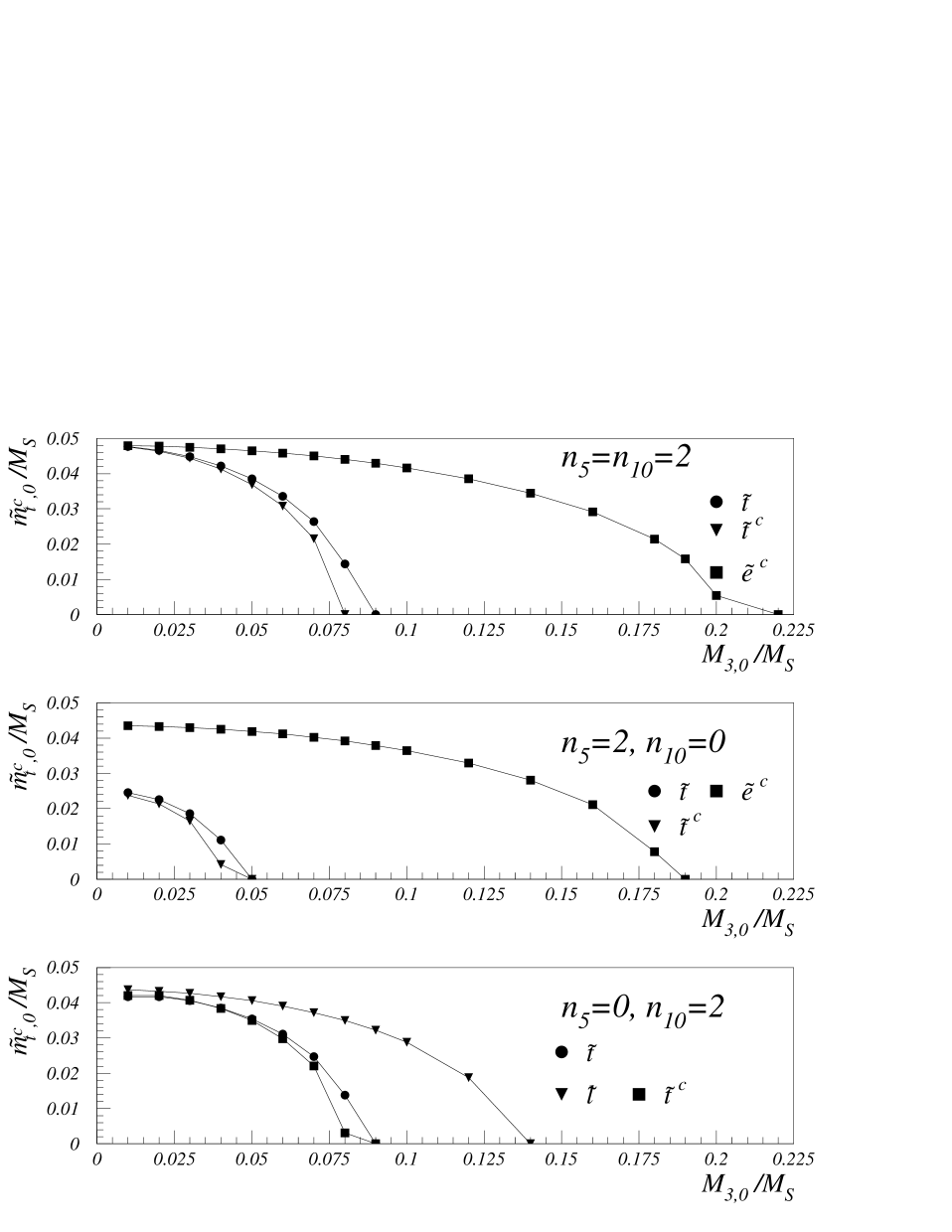
Figure 4.2: Limits for $m_{\tilde{t}^{c},0}/M_{S}$ from the requirement that the stop and slepton (mass)² are positive at the weak scale. The regions below the curves are excluded. Low energy gauge mediated supersymmetry breaking and $\tan\beta=$2.2 are assumed.

The positivity analysis only constrains $m_{\tilde{t}_{i},0}/M_{S}$ for a fixed value of $M_{3,0}/M_{S}$. To directly limit the initial scalar masses some additional information is needed. This is provided by the measured value of $\Delta m_{K}$. If some mixing and degeneracy between the first two generation scalars is assumed, parameterized by $(\delta_{LL},\delta_{RR})$, a minimum value for $M_{S}$ is obtained by requiring that the supersymmetric contribution to $\Delta m_{K}$ does not exceed the measured value. We use the results given in section 4.1 to calculate this minimum value. This result together with the positivity analysis then determines a minimum value for $m_{\tilde{t}^{c},0}$ for a given initial gluino mass $M_{3,0}$. The RG analysis is repeated with $\mu_{S}=M_{S}$, rather than $\mu_{S}$=50 TeV. We only present the results found by assuming GMSB mass relations between the scalars. These results are shown in Fig.4.3. The mass limits for other $\tilde{f}_{i}$ are easily obtained from the information provided in Fig.4.1 and Table 4.2 and are not shown. From Fig.4.3 we find that for $(n_{5},n_{10})$ $=(2,2)$ and a large range of $M_{3,0}$, $m_{\tilde{t}^{c},0}$ must be larger than $7$ TeV for $\sqrt{\delta_{LL}\delta_{RR}}=1$, and larger than $2$ TeV for $\sqrt{\delta_{LL}\delta_{RR}}=0.22$. This results in $c(m_{Z}^{2},m_{\tilde{t},0}^{2})$ of 1500 and 100, respectively. In this case both the squark and selectron limits for $m_{\tilde{t}^{c},0}$ are comparable. The limits for other choices for $\sqrt{\delta_{LL}\delta_{RR}}$ are obtained from Fig.4.3 by a simple scaling, since to a good approximation $\Delta m_{K}\sim\delta_{LL}\delta_{RR}/M^{2}_{S}$. For the cases $(n_{5},n_{10})=(2,0)$ and $(0,2)$, the corresponding limits are much weaker. In the case $(n_{5},n_{10})=(2,0)$, for example, only for $\delta_{RR}\sim 1$ does the constraint that the selectron (mass)${}^{2}>0$ require that $m_{\tilde{t}^{c},0}\sim$1 TeV. The limits for a smaller value of $\delta$ are not shown.

We conclude with some comments about how these results change if $CP$ violation is present in these theories with $O(1)$ phases. Recall from section 4.1 that for the same choice of input parameters, the limit on $M_{S}$ and hence, if the gluino mass is small, the limit on the initial stop mass increases by about a factor of 12. This may be interpreted in one of two ways. Firstly, this constrains those models that were relatively unconstrained by the $\Delta m_{K}$ limit. We concentrate on the models with $n_{5}=2$ and $n_{10}=0$, since this case is the most weakly constrained by the combined $\Delta m_{K}$ and positivity analysis. The conclusions for other models will be qualitatively the same. We find from Fig.4.3 the limit $m_{\tilde{t}^{c},0}>$1 TeV is true only if $\delta_{RR}\sim O(1)$. Smaller values of $\delta_{RR}$ do not require large initial stop masses. From the $CP$ violation constraint, however, smaller values for $\delta_{RR}$ are now constrained. For example, if $\delta_{RR}\sim$ 0.1 and $O(1)$ phases are present, then $m_{\tilde{t}^{c},0}>$1 TeV is required. Secondly, the strong constraint from $\epsilon$ could partially or completely compensate a weakened constraint from the positivity analysis. This could occur, for example, if in an actual model the negative two loop contribution to the stop (mass)² for the same initial input parameters is smaller than the estimate used here. For example, if the estimate of the two loop contribution in an actual model decreases by a factor of $\sim(12.5)^{2}$ and $O(1)$ phases are present, the limit in this case from $\epsilon$ for the same $\delta$ is identical to the values presented in Fig.4.3.

Figure 4.3: Limits for $m_{\tilde{t}^{c},0}$ from the requirement that the stop and slepton (mass)² are positive at the weak scale while suppressing $\Delta m_{K}$, for different values of $(n_{5},n_{10})$, and $(\delta_{LL},\delta_{RR})$. The regions below the curves are excluded. Low energy gauge mediated supersymmetry breaking mass relations and $\tan\beta=$2.2 are assumed.

4.3 High Scale Supersymmetry Breaking

In this section, we consider the case in which SUSY breaking is communicated to the MSSM fields at a high energy scale, that is taken to be $M_{GUT}=2\times 10^{16}$ GeV. In this case, the negative contribution of the heavy scalar soft masses to the soft (mass)² of the light scalars is enhanced by $\sim\ln(M_{GUT}/\hbox{50 TeV})$, since the heavy scalar soft masses contribute to the RGE from $M_{GUT}$ to mass of the heavy scalars. It is clear that as the scale of SUSY breaking is lowered the negative contribution of the heavy scalar soft masses reduces.

This scenario was investigated in reference [43], and we briefly discuss the difference between that analysis and the results presented here. In the analysis of reference [43], the authors made the conservative choice of neglecting $\lambda_{t}$ in the RG evolution. The large value of $\lambda_{t}$ can change the analysis, and it is included here. We find that for some pattern of initial stop and up-type Higgs scalar masses, for example, universal scalar masses, this effect increases the constraint on the stop masses by almost a factor of two. This results in an increase of a factor of $\sim 3-4$ in the amount of fine tuning required to obtain the correct $Z$ mass. Further, in combining the positivity analysis with the constraints from the $\Delta m_{K}$ analysis, the QCD corrections to the Flavour Changing Neutral Current (FCNC) operators have been included, as discussed in section 4.1. In the case $(n_{5},n_{10})=(2,2)$, this effect alone increases the limit on $M_{S}$ and hence the limit on the stop mass by a factor of $\sim 2-3$. The combination of these two elements implies that the positivity constraints can be quite severe.

We proceed as follows. First, we solve the RGE’s from $M_{GUT}$ to $\mu_{S}$ where the heavy scalars are decoupled. At this scale, we add the finite parts of the two loop diagrams. Next, we RG scale (without the heavy scalar terms in the RGE’s) from $\mu_{S}$ to $\mu_{G}$ using these new boundary conditions. Except where stated otherwise, the scales $\mu_{S}$ and $\mu_{G}$ are fixed to be 50 TeV and 1 TeV, respectively.

For $\tilde{f}_{i}\neq\tilde{t}$, $\tilde{t}^{c}$ we find,

$$m^{2}_{\tilde{f}_{i}}(\mu_{G}) = m^{2}_{\tilde{f}_{i,0}}+(2.84C^{i}_{3}+0.639C_{2}^{i}+0.159Y^{2}_{i})M^{2}_{3,0}$$ (4.19)

$$-(4.38C^{i}_{3}+1.92C^{i}_{2}+0.622Y^{2}_{i})\frac{1}{2}(n_{5}+3n_{10})\times 10^{-3}M^{2}_{S}$$

$$-0.829(n_{5}-n_{10})Y_{i}\times 10^{-3}M^{2}_{S}.$$

These results agree with reference [43] for the same choice of input parameters. As in the previous section, the numerical coefficients in Eqn.(4.19) depend on $(n_{5},n_{10})$ through the gauge coupling evolution, and the numbers in Eqn.(4.19) are for $(n_{5},n_{10})=(2,0)$. In Fig.4.4 we plot the values of $m_{\tilde{f}_{i,0}}/M_{S}$ that determine $m^{2}_{\tilde{f}_{i}}(\mu_{G})=0$ as a function of $M_{3}/M_{S}$, for $\tilde{f}_{i}=\tilde{l}_{i}$, $\tilde{q}_{i}$, $\tilde{u}^{c}_{i}$, $\tilde{d}^{c}_{i}$ and $\tilde{e}^{c}_{i}$. We emphasize that the results presented in Fig.4.4 are independent of any further limits that FCNC or fine tuning considerations may imply, and are thus useful constraints on any model building attempts.

Figure 4.4: Limits for $m_{\tilde{f}_{i},0}$ for different values of $(n_{5},n_{10})$ from the requirement that the (mass)² are positive at the weak scale, assuming a supersymmetry breaking scale of $M_{GUT}$. The allowed region lies above all the lines.

For the stops, the numerical solutions to the RGE’s for $\tan\beta=2.2$ are

$$m^{2}_{\tilde{t}}(\mu_{G}) = -0.021A_{t}^{2}+0.068A_{t}M_{3,0}+3.52M^{2}_{3,0}$$

$$-0.142(m^{2}_{H_{u},0}+m^{2}_{\tilde{t}^{c},0})+0.858m^{2}_{\tilde{t},0}-c_{L}0.00567M^{2}_{S},$$

$$m^{2}_{\tilde{t}^{c}}(\mu_{G}) = -0.042A_{t}^{2}+0.137A_{t}M_{3,0}+2.35M^{2}_{3,0}$$

$$-0.283(m^{2}_{H_{u},0}+m^{2}_{\tilde{t},0})+0.716m^{2}_{\tilde{t}^{c},0}-c_{R}0.00259M^{2}_{S},$$

$$m^{2}_{H_{u}}(\mu_{G}) = -0.063A_{t}^{2}+0.206A_{t}M_{3,0}-1.73M^{2}_{3,0}$$ (4.20)

$$-0.425(m^{2}_{\tilde{t},0}+m^{2}_{\tilde{t}^{c},0})+0.574m^{2}_{H_{u},0}+c_{H}0.00218M^{2}_{S},$$

where $(c_{L},c_{R},c_{H})=(1,1,1)$, $(3.9,4.7,4.5)$, $(3,4,3.6)$ for $(n_{5},n_{10})=(2,0)$, $(2,2)$ and $(0,2)$, respectively. The mixed two loop contribution to the RG evolution is $\propto(n_{5}-n_{10})$ and is not negligible. Thus there is no simple relation between the $c$’s for different values of $n_{5}$ and $n_{10}$. From Eqns.(4.2) and (4.1) we find that to keep $m^{2}_{Z}$ fine tuned at less than $1\%$ ($c\leq 100$) in each of the bare parameters, we must have: $\mu\raisebox{-1.72218pt}{\hbox to0.0pt{$\sim$\hss}}\raisebox{1.72218pt}{$<$}$ 500 GeV; $M_{3,0}\raisebox{-1.72218pt}{\hbox to0.0pt{$\sim$\hss}}\raisebox{1.72218pt}{$<$}500$ GeV; $m_{\tilde{t}_{i},0}\raisebox{-1.72218pt}{\hbox to0.0pt{$\sim$\hss}}\raisebox{1.72218pt}{$<$}1$ TeV; and $M_{S}\raisebox{-1.72218pt}{\hbox to0.0pt{$\sim$\hss}}\raisebox{1.72218pt}{$<$}7$ TeV for $(n_{5},n_{10})=(2,2)$. The fine tuning of the $Z$ mass with respect to the heavy scalars is discussed in [42]. Finally, for other values of these parameters the fine tuning increases as $c=100\times\tilde{m}^{2}/\tilde{m}^{2}_{0}$, where $\tilde{m}_{0}$ is the value of $\tilde{m}$ that gives $c=100$.

As in section 4.2, some relations between $m^{2}_{\tilde{t},0}$, $m^{2}_{\tilde{t}^{c},0}$ and $m^{2}_{H_{u},0}$ are needed to obtain a constraint from Eqn.(4.20), using $m^{2}_{\tilde{t}}(\mu_{G})>0$ and $m^{2}_{\tilde{t}^{c}}(\mu_{G})>0$. We discuss both model dependent and model independent constraints on the initial values of the stop masses. The outline of the rest of this section is as follows. First, we assume universal boundary conditions. These results are presented in Fig.4.5. Model independent constraints are obtained by the following. We assume that $m^{2}_{H_{u},0}=0$ and choose $A_{t,0}$ to maximize the value of the stop masses at the weak scale. These results are presented in Fig.4.6. We further argue that these constraints represent minimum constraints as long as $m^{2}_{H_{u},0}\geq 0$. To obtain another set of model independent constraints, we use the electroweak symmetry breaking relation to eliminate $m^{2}_{H_{u},0}$ in favor of $\mu$. Then we present the positivity limits for different values of $\tilde{\mu}/M_{S}$, where $\tilde{\mu}^{2}=\mu^{2}+\frac{1}{2}m^{2}_{Z}$, and assume that
$m^{2}_{H_{d},0}=0$ to minimize the value of $\mu$. These limits are model independent and are presented in Fig.4.7, for the case $n_{5}=n_{10}=2$. We then combine these analyses with the limits on $M_{S}$ obtained from $\Delta m_{K}$. We conclude with some discussion about the anomalous $D-$term solutions to the flavor problem.

We first consider universal boundary conditions for the stop and Higgs masses. That is, we assume that $m^{2}_{\tilde{t},0}=m^{2}_{\tilde{t}^{c},0}=m^{2}_{H_{u},0}=\tilde{m}^{2}_{0}$. In Fig.4.5 we plot for $\tan\beta=2.2$ the minimum value of $\tilde{m}_{0}/M_{S}$ required to maintain $m^{2}_{\tilde{t}}(\mu_{G})>0$ and $m^{2}_{\tilde{t}^{c}}(\mu_{G})>0$. This value of $\tan\beta$ corresponds to $\lambda_{t}(M_{GUT})=0.88$, in the case that $(n_{5},n_{10})=(2,0)$. For comparison, the results gotten assuming $\lambda_{t}=0$ may be found in reference [43]. For $n_{5}=n_{10}=2$ we note from Fig.4.5 that if $M_{S}=$ 20 TeV and the gaugino masses are small, the limit on the stop mass is $m_{\tilde{t}^{c},0}\geq$ 6 TeV. This limit is weakened to 5.6 TeV if $M_{3,0}\raisebox{-1.72218pt}{\hbox to0.0pt{$\sim$\hss}}\raisebox{1.72218pt}{$<$}$ 300 GeV is allowed. Even in this case, this large initial stop mass requires a fine tuning that is $c\sim(\hbox{5.6 TeV})^{2}/m^{2}_{Z}\sim$ 3700, i.e., a fine tuning of $\sim 10^{-3}$ is needed to obtain the correct $Z$ mass.

We now assume $m^{2}_{H_{u},0}=0$ and choose the initial value of $A_{t,0}$ to maximize the value of $m^{2}_{\tilde{t}_{i}}(\mu_{G})$. The values of $m^{2}_{\tilde{t},0}$ and $m^{2}_{\tilde{t}^{c},0}$ are chosen such that $m^{2}_{\tilde{t}}(\mu_{G})>0$ and $m^{2}_{\tilde{t}^{c}}(\mu_{G})>0$. We note that in this case the constraint is weaker because the $\lambda_{t}$ contribution to the RG evolution of the stop (mass)² is less negative. These results are plotted in Fig.4.6.

We discuss this case in some more detail and argue that the minimum value of $m_{\tilde{t}_{i},0}$ obtained in this way will be valid for all $m^{2}_{H_{u}}\geq 0$ and all $A_{t,0}$. Eliminate the $A_{t,0}$ term by choosing $A_{t,0}=kM_{3,0}$ such that the $A_{t}$ contributions to $m^{2}_{\tilde{t}_{i}}(\mu_{G})$ is maximized. Other choices for $A_{t,0}$ require larger values for $m^{2}_{\tilde{t}_{i},0}$ to maintain $m^{2}_{\tilde{t}_{i}}(\mu_{G})=0$. The value of $k$ is determined by the following. A general expression for the value of the soft masses of the stops at the weak scale is

$$m^{2}_{\tilde{t}}(\mu_{G})=-aA^{2}_{t,0}+bA_{t,0}M_{3,0}+cM^{2}_{3,0}+\cdots,$$ (4.21)

$$m^{2}_{\tilde{t}^{c}}(\mu_{G})=-2aA^{2}_{t,0}+2bA_{t,0}M_{3,0}+dM^{2}_{3,0}+\cdots,$$ (4.22)

with $a$, $c$ and $d$ positive. The maximum value of $m^{2}_{\tilde{t}_{i}}(\mu_{G})$ is obtained by choosing $A_{t,0}=bM_{3,0}/2a$. The value of the stops masses at this choice of $A_{t,0}$ are

$$m^{2}_{\tilde{t}}(\mu_{G})=(c+\frac{b^{2}}{4a})M^{2}_{3,0}+\cdots,$$ (4.23)

$$m^{2}_{\tilde{t}^{c}}(\mu_{G})=(d+2\frac{b^{2}}{4a})M^{2}_{3,0}+\cdots.$$ (4.24)

An inspection of Eqn.(4.20) gives $b=0.068$ and $a=0.021$ for $\tan\beta=2.2$. In this case the ‘best’ value for $A_{t,0}$ is $A^{B}_{t,0}\sim 1.6M_{3,0}$. It then follows that the quantity $b^{2}/4a=0.055$ is a small correction to the coefficient of the gaugino contribution in Eqn.(4.20). Thus the difference between the minimum initial stop masses for $A_{t,0}=0$ and $A_{t,0}$= $A^{B}_{t,0}$ is small. Next assume that $m^{2}_{H_{u},0}=0$. Requiring both $m^{2}_{\tilde{t}}(\mu_{G})=0$ and $m^{2}_{\tilde{t}^{c}}(\mu_{G})=0$ determines a minimum value for $m^{2}_{\tilde{t},0}$ and $m^{2}_{\tilde{t}^{c},0}$. Now since the $m^{2}_{H_{u},0}$ contribution to both the the stop soft (mass)² is negative (see Eqn.(4.20)), the minimum values for $m^{2}_{\tilde{t}_{i},0}$ found by the preceeding procedure are also minimum values if we now allow any $m^{2}_{H_{u},0}>0$.

We conclude that for all $A_{t,0}$ and all $m^{2}_{H_{u},0}\geq 0$, the limits presented in Fig.4.6 represent lower limits on the initial stop masses if we require that the soft (mass)² remain positive at the weak scale. Further, the limits in this case are quite strong. For example, from Fig.4.6 we find that if $M_{S}\sim$ 20 TeV and $M_{3,0}\sim$ 200 GeV (so that $M_{3,0}/M_{S}\sim$10${}^{-2})$, then the initial stop masses must be greater than 3.5 TeV in the case that $(n_{5},n_{10})=(2,2)$ The results are stronger in a more realistic scenario, i.e., with $m_{H_{u},0}^{2}>0$. If, for example, $m^{2}_{H_{u},0}\sim m^{2}_{\tilde{t}^{c},0}/9$ the constraints are larger by only a few percent. In the case that $m^{2}_{H_{u},0}=m^{2}_{\tilde{t}^{c},0}=m^{2}_{\tilde{t},0}$, presented in Fig.4.5, however, the constraint on the initial $\tilde{t}^{c}$ mass increases by almost a factor of two.

To obtain constraints on the initial stop masses we have thus far had to assume some relation between $m^{2}_{H_{u},0}$ and $m^{2}_{\tilde{t}^{c},0}$, for example, $m^{2}_{H_{u},0}=0$ or $m^{2}_{H_{u},0}=m^{2}_{\tilde{t}^{c},0}$. Perhaps a better approach is to use the EWSB relation, Eqn.(4.2), to eliminate $m^{2}_{H_{u},0}$ in favor of $\mu^{2}$. This has the advantage of being model independent. It is also a useful reorganization of independent parameters since the amount of fine tuning required to obtain the correct $Z$ mass increases as $\mu$ is increased. To obtain some limits we choose $m_{H_{d},0}^{2}=0$ to minimize the value of $\mu^{2}$, and require that $m^{2}_{H_{u},0}$ is positive. The minimum value of $m_{\tilde{t}^{c},0}/M_{S}$ and $m_{\tilde{t},0}/M_{S}$ for different choices of $\tilde{\mu}/M_{S}$ are gotten by solving $m^{2}_{\tilde{t}^{c}}(\mu_{G})=0$ and $m^{2}_{\tilde{t}}(\mu_{G})=0$. These results are presented in Fig.4.7. In this Figure the positivity constraints terminate at that value of $M_{3,0}$ which gives $m^{2}_{H_{u},0}=0$.

As discussed above, reducing the value of $m^{2}_{H_{u},0}$ decreases the positivity limit on $m_{\tilde{t}_{i},0}$. Consequently the fine tuning of $m_{Z}$ with respect to $m_{\tilde{t}_{i},0}$ is also reduced. But using Eqns.(4.20) and (4.2), it can be seen that decreasing $m_{H_{u},0}^{2}$ while keeping $m_{\tilde{t}^{c}}^{2}(\mu_{G})=0$ and $m_{\tilde{t}}^{2}(\mu_{G})=0$ results in a larger $\mu$, thus increasing the fine tuning with respect to $\mu$. This can also be seen from Fig.4.7. We find, for example, that if $M_{3,0}/M_{S}\sim 0.01$, the small value $\tilde{\mu}/M_{S}=0.01$ requires $m_{\tilde{t}_{i},0}/M_{S}\sim 0.25$. For $M_{S}=10$ TeV, this corresponds to $\mu\sim$ 100 GeV and $m_{\tilde{t}_{i},0}\geq$ 2.5 TeV. A further inspection of Fig.4.7 shows that for the same value of $M_{3,0}/M_{S}$, a value of $m_{\tilde{t},0}/M_{S}=0.17$ is allowed (by reducing $m^{2}_{H_{u},0}$) only if $\tilde{\mu}/M_{S}$ is increased to 0.14. This corresponds to $\mu=1.4$ TeV for $M_{S}=10$ TeV; this implies that $c(m^{2}_{Z};\mu)\sim 930$. We find that the limit on the initial stop masses can only be decreased at the expense of increasing $\mu$.

Finally, the limits become weaker if $m^{2}_{H_{u},0}<0$. This possibility is theoretically unattractive on two accounts. Firstly, a nice feature of supersymmetric extensions to the SM is that the dynamics of the model, through the presence of the large top quark Yukawa coupling, naturally leads to the breaking of the electroweak symmetry [12]. This is lost if electroweak symmetry breaking is already present at the tree level. Secondly, the fine tuning required to obtain the correct $Z$ mass is increased. From Fig.4.7 we infer that while reducing $m^{2}_{H_{u},0}$ below zero does reduce the limit on the initial stop masses, the value of $\mu$ increases beyond the values quoted in the previous paragraph, thus futher increasing the fine tuning of the $Z$ mass. This scenario is not discussed any further.

Figure 4.5: Limits for $\tilde{m}_{0}/M_{S}$ from the requirement that the stop (mass)² are positive at the weak scale, for $\tan\beta=2.2$, $A_{t,0}=0$ and assuming universal scalar masses at $M_{GUT}$ for the stop and Higgs scalars. The region below the curves are excluded.

Figure 4.6: Limits for $m_{\tilde{t},0}/M_{S}$, $m_{\tilde{t}^{c},0}/M_{S}$, from the requirement that the stop (mass)² are positive at the weak scale, for $M_{SUSY}=M_{GUT}$, $\tan\beta=2.2$ and assuming that $m^{2}_{H_{u},0}=0.$ The value of $A_{t,0}$ is chosen to maximize the value of the stop soft masses at the weak scale. The region below the curves are excluded.

Figure 4.7: Limits for $m_{\tilde{t},0}/M_{S}$, $m_{\tilde{t}^{c},0}/M_{S}$, from the requirement that the stop (mass)² are positive at the weak scale, for $(n_{5},n_{10})=(2,2)$, $M_{SUSY}=M_{GUT}$, $\tan\beta=2.2$, and different values of $\tilde{\mu}/M_{S}$. The contours end at that value of $M_{3,0}/M_{S}$ that gives $m_{H_{u},0}/M_{S}=0$. The value of $A_{t,0}$ is chosen to maximize the value of the stop soft masses at the weak scale.

We now combine the positivity analysis of this section with the results of section 4.1 to place lower limits on the soft scalar masses. For given values of $\delta_{LL},\delta_{RR}$, a minimum value of $M_{S}$, $M_{S,min}$, is found using the results of section 4.1. This is combined with the positivity analysis in Fig.4.6, to produce the results shown in Fig.4.8. We also show other limits gotten by assuming $m^{2}_{H_{u},0}=m^{2}_{\tilde{t}^{c},0}$. These results are presented in Fig.4.9. In Fig.4.10 we also present the stop mass limits for different values of $\mu$, and restrict to $m^{2}_{H_{u},0}\geq 0$ and $\sqrt{\delta_{LL}\delta_{RR}}=0.04$. In all cases the heavy scalars were decoupled at $M_{S,min}$, rather than 50 TeV, and so the positivity analysis was repeated. The value of $A_{t,0}$ was chosen to maximize the value of the stop masses at the weak scale. For completeness, the results for the cases $(n_{5},n_{10})=(2,0)$ and $(0,2)$ and $m^{2}_{H_{u},0}=0$ are presented in Fig.4.11. We repeat that the minimum allowable values for the stop masses consistent with $m^{2}_{H_{u},0}>0$, gotten by setting $m^{2}_{H_{u},0}=0$, are given in Figs.4.8 and 4.11.

We next briefly discuss some consequences of this numerical analysis. We concentrate on the case $n_{5}=n_{10}=2$, since this is the relevant case to consider if the supersymmetric flavor problem is solved by decoupling the heavy scalars. Other choices for $n_{5}$ and $n_{10}$ require additional physics to explain the required degeneracy or alignment of any light non-third generation scalars. From Figs.4.8 and 4.9 we find that for $\sqrt{\delta_{LL}\delta_{RR}}=0.22$ and $M_{3,0}\leq$ 1 TeV, $m_{\tilde{t}_{i},0}>$7 TeV is required. If instead we restrict both $c(m^{2}_{Z};M^{2}_{S})$ and $c(m^{2}_{Z};M^{2}_{3,0})$ to be less than 100, then we must have $M_{S}\raisebox{-1.72218pt}{\hbox to0.0pt{$\sim$\hss}}\raisebox{1.72218pt}{$<$}$ 7 TeV and $M_{3,0}\raisebox{-1.72218pt}{\hbox to0.0pt{$\sim$\hss}}\raisebox{1.72218pt}{$<$}$ 500 GeV. To not be excluded by $\Delta m_{K}$, we further require that $\sqrt{\delta_{LL}\delta_{RR}}\leq 0.04$ which leads to a fine tuning of one part in $\sim 2/\delta$ , i.e., $\sim 50$. An inspection of Figs.4.8 and 4.9 implies that for $\sqrt{\delta_{LL}\delta_{RR}}\approx 0.04$, $m_{\tilde{t},0}$ must be larger than 0.9$-$1.3 TeV, depending on the value of $m^{2}_{H_{u},0}$. Alternatively, if we also restrict $\mu\leq$ 500 GeV, then from Fig.4.10 we find that $m_{\tilde{t}_{i},0}\geq$ 800 GeV. Thus $c(m^{2}_{Z};m^{2}_{\tilde{t}_{i},0})=64-170$. This fine tuning can be reduced only by increasing the $c(m^{2}_{Z})$’s for the other parameters to more than 100 (or by increasing the fine tuning of $\delta$ to more than one part in 50). We conclude that unless $\sqrt{\delta_{RR}\delta_{LL}}$ is naturally small, decoupling the heavy scalars does not provide a natural solution to the flavor problem.

Figure 4.8: Limits for $m_{\tilde{t},0}$ and $m_{\tilde{t}^{c},0}$, $m_{\tilde{e}^{c}}$, and $m_{\tilde{l}}$ from the requirement that the (mass)² are positive at the weak scale while suppressing $\Delta m_{K}$. It was assumed that $M_{SUSY}=M_{GUT}$, $\tan\beta=2.2$ and that $m^{2}_{H_{u},0}=0.$ The value of $A_{t,0}$ was chosen to maximize the value of the stop soft masses at the weak scale. The heavy scalars were decoupled at the minimum value allowed by $\Delta m_{K}$.

Figure 4.9: Limits for $m_{\tilde{t},0}$ and $m_{\tilde{t}^{c},0}$ from the requirement that the stop (mass)² are positive at the weak scale while suppressing $\Delta m_{K}$. It was assumed that $M_{SUSY}=M_{GUT}$, $\tan\beta=2.2$ and that $m^{2}_{H_{u},0}=m^{2}_{\tilde{t}^{c},0}.$ The value of $A_{t,0}$ was chosen to maximize the value of the stop soft masses at the weak scale. The heavy scalars were decoupled at the minimum value allowed by $\Delta m_{K}$.

Figure 4.10: Limits for $m_{\tilde{t},0}$ and $m_{\tilde{t}^{c},0}$ from the requirement that the stop (mass)² are positive at the weak scale while suppressing $\Delta m_{K}$, for $(n_{5},n_{10})=(2,2)$, $\sqrt{\delta_{LL}\delta_{RR}}=0.04$, and different values of $\mu$. The contours terminate at $m^{2}_{H_{u},0}=0$. It was assumed that $M_{SUSY}=M_{GUT}$ and $\tan\beta=2.2$. The value of $A_{t,0}$ was chosen to maximize the value of the stop soft masses at the weak scale. The heavy scalars were decoupled at the minimum value allowed by $\Delta m_{K}$.

Figure 4.11: Limits for $m_{\tilde{t},0}$, $m_{\tilde{t}^{c},0}$ from the requirement that the stop (mass)² are positive at the weak scale while suppressing $\Delta m_{K}$, for the cases $(n_{5},n_{10})=(2,0)$ and $(0,2)$. It was assumed that $M_{SUSY}=M_{GUT}$, $\tan\beta=2.2$ and that $m^{2}_{H_{u},0}=0.$ The value of $A_{t,0}$ was chosen to maximize the value of the stop soft masses at the weak scale. The heavy scalars were decoupled at the minimum value allowed by $\Delta m_{K}$.

To conclude this section we discuss the constraint this analysis implies for those models which generate a split mass spectrum between the third and the first two generations through the $D$-term contributions of an anomalous $U(1)$ gauge symmetry [37, 40, 41]. These models can “explain” the hierarchy of the Yukawa couplings. In the model of set D of [40], the two ${\bf\bar{5}}$’s of the first two generations are at $7$ TeV and $6.1$ TeV and the two ${\bf 10}$’s are at $6.1$ and $4.9$ TeV, respectively, so that $\Delta m_{K}$ is suppressed. These values must be increased by a factor of 2.5 to correct for the QCD enhancement of the SUSY contribution to $\Delta m_{K}$, as discussed in section 4.1. To obtain a conservative bound on the initial stop masses from the positivity requirement, we first assume that all the heavy scalars have a common mass $M_{S}=2.5\times 5$TeV$=12.5$ TeV. (It would have been 5 TeV without the QCD correction.) Then assuming a weak scale value of the gluino mass which is less than $1.5$ TeV (so that $c(m^{2}_{Z},M^{2}_{3,0})$ is less than 100) and setting $m^{2}_{H_{u},0}=0$ $(m^{2}_{\tilde{t}^{c},0})$, we find from Fig.4.6 $($4.5$)$ that $m_{\tilde{t},0}\geq 2.0$ $(3.4)$ TeV is required. This leads to $c(m^{2}_{Z};m^{2}_{\tilde{t},0})\geq 400$ $(1100)$. To obtain a better bound, we repeat our analysis using $n_{5}m^{2}_{5}+\hbox{3}n_{10}m^{2}_{10}=((\hbox{7 TeV})^{2}+(\hbox{6.1 TeV})^{2}+\hbox{3}\times(\hbox{6.1 TeV})^{2}+\hbox{3}\times(\hbox{4.9 TeV})^{2})\times(\hbox{2.5})^{2}$. It is possible to do this since only this combination appears in the RG analysis for $(n_{5},n_{10})=(2,2)$. We find (assuming $m_{H_{u},0}^{2}=0$ and the gluino mass at the weak scale is less than $1.5$ TeV) that $m_{\tilde{t},0}\stackrel{{\scriptstyle>}}{{\sim}}3$ TeV. In the model of [41], $\delta_{RR}\approx\delta_{LL}\approx 0.01$. To obtain a limit on the initial stop masses, we use the bound obtained from either Figs.4.8 or 4.9 for $\delta_{RR}=\delta_{LL}\approx 0.04$, and divide the limit by a factor of 4. By inspecting these Figures we find that this model is only weakly constrained, even if $m^{2}_{H_{u},0}\sim m^{2}_{\tilde{t},0}$. We now discuss the limits in this model when $O(1)$ $CP$ violating phases are present. To obtain the minimum value of $M_{S}$ in this case, we should multiply the minimum value of $M_{S}$ obtained from the $\Delta m_{K}$ constraint for $\delta_{LL}=\delta_{RR}=0.04$ by 12.5/4; dividing by 4 gives the result for $\delta_{LL}=\delta_{RR}=0.01$ and multiplying by 12.5 gives the constraint on $M_{S}$ from $\epsilon$. The result is $M_{S}\raisebox{-1.72218pt}{\hbox to0.0pt{$\sim$\hss}}\raisebox{1.72218pt}{$>$}$ 23 TeV. Next, we assume that $M_{3,0}$ is less than 600 GeV, so that the value of the gluino mass at the weak scale is less than $\sim$ 1.5 TeV. This gives $M_{3,0}/M_{S}\leq 0.026$. Using these values of $M_{3,0}$ and $M_{S}$, an inspection of Figs.4.5 and 4.6 implies that $m_{\tilde{t},0}$ must be larger than 3.9 TeV to 6.7 TeV, depending on the value of $m^{2}_{H_{u},0}$. This gives $c(m^{2}_{Z};m^{2}_{\tilde{t},0})\geq 1600$. In the model of [37], $M_{3,0}/M_{S}\approx 0.01$ and $m_{\tilde{f},0}/M_{S}\approx 0.1$. Inspecting Figs.4.5 and 4.6 we find that these values are excluded for $(n_{5},n_{10})=(2,2)$ and $(0,2)$. The case $(2,0)$ is marginally allowed. The model of [37] with $(n_{5},n_{10})=(2,2)$ and $\lambda_{t}=0$ was also excluded by the analysis of reference [43].

4.4 Conclusions

In this chapter we have studied whether the SUSY flavor problem can be solved by making the scalars of the first and second generations heavy, with masses $M_{S}$ ($\stackrel{{\scriptstyle>}}{{\sim}}$few TeV), without destabilising the weak scale. If the scale, $M_{SUSY}$, at which SUSY breaking is mediated to the SM scalars is close to the GUT scale, then the heavy scalars drive the light scalar (in particular the stop) (mass)² negative through two loop RG evolution. In order to keep the (mass)² at the weak scale positive, the initial value of the stop (and other light scalar) soft masses, $m_{\tilde{f}_{i},0}$, must typically be $\stackrel{{\scriptstyle>}}{{\sim}}1$ TeV, leading to fine tuning in EWSB. We included two new effects in this analysis: the effect of $\lambda_{t}$ in the RGE’s which makes the stop (mass)² at the weak scale more negative and hence makes the constraint on the initial value stronger, and the QCD corrections to the SUSY box diagrams which contribute to $K-\bar{K}$ mixing.

Some results of our analysis for $M_{SUSY}=M_{GUT}$ can be summarized as follows. We restrict the gluino mass (at the weak scale) to be less than about $1.5$ TeV, so that the fine tuning of $m^{2}_{Z}$ with respect to the bare gluino mass, $M_{3,0}$, is not worse than $1\%$. This requires that $M_{3,0}\raisebox{-1.72218pt}{\hbox to0.0pt{$\sim$\hss}}\raisebox{1.72218pt}{$<$}600$ GeV. We also assume that $m_{H_{u},0}^{2}=0$ to maximize the value of the stop masses at the weak scale. We find that if $\sqrt{\delta_{LL}\delta_{RR}}=0.22$ then $M_{S}\geq$ 40 TeV is required to be consistent with $\Delta m_{K}$. With these assumptions, this implies that for $M_{3,0}$ less than 1 TeV, $m_{\tilde{t}_{i},0}>$ 6.5 TeV is needed to not break color and charge at the weak scale. Even for $\sqrt{\delta_{LL}\delta_{RR}}=0.04$, we find that we need $M_{S}\stackrel{{\scriptstyle>}}{{\sim}}7$ TeV. This implies that $m_{\tilde{t},0}>1$ TeV is required if $M_{3,0}\leq$ 500 GeV. This results in a fine tuning of $1\%$. For $\delta_{LL}=1$ and $\delta_{RR}=0$, we find that $M_{S}\stackrel{{\scriptstyle>}}{{\sim}}30$ TeV and $m_{\tilde{t},0}>4$ TeV. For $\delta_{LL}=0.22$ and $\delta_{RR}=0$, we find that $M_{S}\stackrel{{\scriptstyle>}}{{\sim}}7$ TeV and $m_{\tilde{t},0}>1$ TeV (this holds for an initial gluino mass less than about $300$ GeV). For $\delta_{LL}=0$ and $\delta_{RR}=1$, we find that $M_{S}\stackrel{{\scriptstyle>}}{{\sim}}30$ TeV and $m_{\tilde{t}^{c},0}>2$ TeV. The constraints are weaker for smaller values of $\delta$. In a realistic model, $m_{H_{u},0}^{2}$ might be comparable to $m_{\tilde{t},0}^{2}$ and the constraints on $m_{\tilde{t},0}$ in this case are stronger. This is also discussed. We note that independent of the constraint from $K-\bar{K}$ mixing, our analysis can be used to check the phenomenological viability of any model that has heavy scalars. We also discuss the phenomenological viability of the anomalous $D-$term solution, and find it to be problematic.

We then considered the possibility that $M_{SUSY}=M_{S}$. In this case, there is no RG log enhancement of the negative contribution of the heavy scalar masses to the light scalar (mass)². For this case, we computed the finite parts of the two loop diagrams and used these results as estimates of the two loop contribution of the heavy scalars to the light scalar soft (mass)². We then combined these results with the constraints from $K-\bar{K}$ mixing to obtain lower limits on the boundary values of the stop mass. As an example, we assumed gauge mediated SUSY breaking boundary conditions for the light scalars. If $n_{5}\neq n_{10}$ then one of the selectron masses, rather than the stop masses, provides the stronger constraint on $m_{\tilde{t}_{i},0}$ once gauge mediated boundary conditions are used to relate $m_{\tilde{e}^{c},0}$ and $m_{\tilde{l},0}$ to $m_{\tilde{t}_{i},0}$. Some of our results can be summarized as follows. We restrict the gluino mass at the weak scale to be less than about $3$ TeV, again to avoid more than $2\%$ fine tuning of $m^{2}_{Z}$ with respect to the gluino mass. For $\sqrt{\delta_{LL}\delta_{RR}}=0.22$ we find that $m_{\tilde{t}_{i},0}\geq$ 1 TeV is required. The fine tuning of $m^{2}_{Z}$ with respect to the stop mass is $\sim 3\%$ in this case. For the cases $\delta_{LL}=0$ and $\delta_{RR}=1$, and $\delta_{LL}=1$ and $\delta_{RR}=0$ we find that $m_{\tilde{t},0}\stackrel{{\scriptstyle>}}{{\sim}}1$ TeV. As before, the constraints on $m_{\tilde{t},0}$ for smaller values of $\delta$ are weaker than $\sim 1$ TeV. Again, we emphasize that the constraints in an actual model of this low energy supersymmetry breaking scenario could be different, and our results should be treated as estimates only. Finally, we also briefly discuss the $CP$ violating constraints from $\epsilon$, and find that all these limits increase by a factor of $\sim 12$ if $O(1)$ phases are present.

Chapter 5 Summary

In this thesis, we studied some fine tuning and naturalness issues in the supersymmetric Standard Model (SSM). SUSY solves the gauge hierarchy problem of the SM, if the superpartners of the SM particles are at the weak scale: the Higgs (mass)² is stabilized at the scale of the SUSY breaking masses of the superpartners and is negative due to the large top quark Yukawa coupling. Therefore, electroweak symmetry breaking occurs naturally. However, we argued that constraints from phenomenology (the ones we discuss all come from FCNC’s) require that, unless we add some global symmetries to the SSM, there is some degree of fine tuning/unnaturalness in some (other) sector of the SSM (in some cases, the fine tuning of the weak scale is reintroduced).

We showed that supersymmetric $R$-parity breaking ($\not\!\!R_{p}$) interactions always result in Flavor Changing Neutral Current (FCNC) processes. Within a single coupling scheme, these processes can be avoided in either the charge $+2/3$ or the charge $-1/3$ quark sector, but not both. These processes were used to place constraints on $\not\!\!R_{p}\,$ couplings. The constraints on the first and the second generation couplings are better than those existing in the literature. Thus, we have to either impose $R$-parity or tolerate some unnaturalness in the form of small values of the $R$-parity violating couplings.

Non-degenerate squarks and sleptons of especially the first two generations lead to FCNC’s; this is the SUSY flavor problem. If SUSY is mediated by gravity (supergravity theories), then we have to either fine tune the scalar masses to give the required degeneracies or introduce flavor symmetries or quark-squark alignment. Another way of communicating SUSY breaking to the sparticles is by the SM gauge intercations. In this case, scalars with the same gauge quantum numbers are degenerate leading to very small SUSY contributions to FCNC’s.

However, the models of low energy gauge mediation predict a large hierarchy in the scalar mass spectrum resulting in a large and negative value for the Higgs soft (mass)² at the weak scale. This means that the $\mu$ term has to be fine tuned to give the correct $Z$ mass. We found that if LEP2 does not discover SUSY, then these models would lead to a $7\%$ fine tuning. We constructed a model with a non-minimal messenger sector (more messenger $SU(2)_{w}$ doublets than $SU(3)_{c}$ triplets) which reduced the fine tuning to $\sim 40\%$. Our model has some extra vector-like quarks (to maintain gauge coupling unification) which get a mass at the weak scale from a coupling to a singlet. We used the same singlet to generate the $\mu$ and $B\mu$ Higgs masses by coupling it to the Higgs doublets. This model requires $\sim 25\%$ fine tuning. We showed that these models with the split $({\bf 5}+{\bf\bar{5}})$ messenger fields can be derived from a $SU(5)\times SU(5)$ GUT using a doublet-triplet splitting mechanism.

The SUSY flavor problem can also be solved by making the scalars of the first two generations heavy (with mass $M_{S}\stackrel{{\scriptstyle>}}{{\sim}}$few TeV). A priori, this does not result in any fine tuning in EWSB since only the stop mass has to be smaller than $\sim 1$ TeV to get the weak scale naturally. However, the heavy scalars drive the light scalar (in particular the stop) (mass)² negative through two loop Renormalization Group Equations (RGE), if the scale at which SUSY breaking is mediated to the sparticles ($M_{SUSY}$) is high (say the GUT scale). Thus, the boundary value of the stop mass has to be large to avoid negative stop (mass)² at the weak scale, in turn, leading to fine tuning in EWSB. Two new effects were included in our analysis: the effect of the top quark Yukawa coupling in the RGE which makes the constraint on the stop mass stronger since it makes the stop (mass)² more negative, and the QCD corrections to the SUSY contributions to $K-\bar{K}$ mixing. Even with a degeneracy between the squarks of the first two generations of the order of the Cabibbo angle, i.e., $\sim 0.22$, these squarks must be heavier than $\sim 40$ TeV to suppress $\Delta m_{K}$. This implies, in the case of a high scale of supersymmetry breaking, that the boundary value of the stop mass has to be greater than $\sim 7$ TeV to keep the stop (mass)² positive at the weak scale.

We also studied the case where $M_{SUSY}$ is of the order of the mass of the heavy scalars. We computed the finite parts of the same two loop diagrams and used these as estimates of the two loop contribution of the heavy scalar masses to the stop (mass)². It was found that for mixing between the squarks of the order of the Cabibbo angle, the stop mass at the boundary needs to be larger than $\sim 2$ TeV to avoid negative stop (mass)² at the weak scale. Thus, for both cases, the large boundary value of the stop masses ($\stackrel{{\scriptstyle>}}{{\sim}}1$ TeV) reintroduces fine tuning in electroweak symmetry breaking.

Appendix A Fine Tuning Functions

In this appendix the Barbieri-Giudice fine tuning parameters for both the MSSM and NMSSM in a gauge mediated SUSY breaking scenario are presented.

In an MSSM with gauge mediated SUSY breaking, the fundamental parameters of the theory (in the visible sector) are: $\Lambda_{mess}$, $\lambda_{t}$, $\mu$, and $\mu^{2}_{3}$. Once electroweak symmetry breaking occurs, the extremization conditions determine both $m^{2}_{Z}$ and $\tan\beta$ as a function of these parameters. To measure the sensitivity of $m^{2}_{Z}$ to one of the fundamental parameters $\lambda_{i}$, we compute the variation in $m^{2}_{Z}$ induced by a small change in one of the $\lambda_{i}$. The quantity

$$\frac{\delta m^{2}_{Z}}{m^{2}_{Z}}\equiv c(m^{2}_{Z};\lambda_{i})\frac{\delta\lambda_{i}}{\lambda_{i}},$$ (A.1)

where

$$c(m^{2}_{Z};\lambda_{i})=\frac{\lambda_{i}}{m^{2}_{Z}}\frac{\partial m^{2}_{Z}}{\partial\lambda_{i}},$$ (A.2)

measures this sensitivity [14]. In the case of gauge mediated SUSY breaking models, there are four functions $c(m^{2}_{Z};\lambda_{i})$ to be computed. They are:

$$c(m^{2}_{Z};\mu^{2})=\frac{2\mu^{2}}{m^{2}_{Z}}\left(1+\frac{\tan^{2}\beta+1}{(\tan^{2}\beta-1)^{2}}\frac{4\tan^{2}\beta(\tilde{\mu}^{2}_{1}-\tilde{\mu}^{2}_{2})}{(\tilde{\mu}^{2}_{1}-\tilde{\mu}^{2}_{2})(\tan^{2}\beta+1)-m^{2}_{Z}(\tan^{2}\beta-1))}\right),$$ (A.3)

$$c(m^{2}_{Z};\mu^{2}_{3}) = 4\tan^{2}\beta\frac{\tan^{2}\beta+1}{(\tan^{2}\beta-1)^{3}}\frac{\tilde{\mu}^{2}_{1}-\tilde{\mu}^{2}_{2}}{m^{2}_{Z}}$$ (A.4)

$$\approx \frac{4}{\tan^{2}\beta}\frac{\tilde{\mu}^{2}_{1}-\tilde{\mu}^{2}_{2}}{m^{2}_{Z}},\;\;\hbox{for large}\;\tan\beta,$$

$$c(m^{2}_{Z};\lambda_{t}) = 2\frac{\lambda_{t}^{2}}{m_{Z}^{2}}\frac{\partial m_{Z}^{2}}{\partial m_{H_{u}}^{2}}\frac{\partial m_{H_{u}}^{2}}{\partial\lambda_{t}^{2}}$$ (A.5)

$$= \frac{4}{m^{2}_{Z}}\lambda^{2}_{t}\frac{\tan^{2}\beta}{\tan^{2}\beta-1}\frac{\partial m^{2}_{H_{u}}}{\partial\lambda^{2}_{t}}\left(1+2\frac{\tilde{\mu}^{2}_{1}-\tilde{\mu}^{2}_{2}}{\tilde{\mu}^{2}_{1}+\tilde{\mu}^{2}_{2}}\frac{\tan^{2}\beta+1}{(\tan^{2}\beta-1)^{2}}\right)$$

$$\approx \frac{4}{m^{2}_{Z}}\frac{\partial m^{2}_{H_{u}}}{\partial\lambda^{2}_{t}},\;\;\;\hbox{for large}\;\tan\beta.$$

This measures the sensitivity of $m^{2}_{Z}$ to the electroweak scale value of $\lambda_{t}$, $\lambda_{t}(m_{weak})$. The Yukawa coupling $\lambda_{t}(m_{weak})$ is not, however, a fundamental parameter of the theory. The fundamental parameter is the value of the coupling at the cutoff $\Lambda^{0}=M_{GUT}$ or $M_{Pl}$ of the theory. We really should be computing the sensitivity of $m^{2}_{Z}$ to this value of $\lambda_{t}$. The measure of sensitivity is then correctly given by

$$c(m^{2}_{Z};\lambda_{t}(\Lambda^{0})) = \frac{\lambda_{t}(\Lambda^{0})}{\lambda_{t}(m_{weak})}c(m^{2}_{Z};\lambda_{t}(m_{weak}))\frac{\partial\lambda_{t}(m_{weak})}{\partial\lambda_{t}(\Lambda^{0})}.$$ (A.6)

We remark that for the model discussed in the text with three $l+\bar{l}$ and one $q+\bar{q}$ messenger fields, the numerical value of $(\lambda_{t}(\Lambda^{0})/\lambda_{t}(m_{weak}))\partial\lambda_{t}(m_{weak})/\partial\lambda_{t}(\Lambda^{0})$ is typically $\sim 0.1$ because $\lambda_{t}(m_{weak})$ is attracted to its infra-red fixed point. This results in a smaller value for $c(m^{2}_{Z};\lambda_{t})$ than is obtained in the absence of these considerations.

With the assumption that $m_{H_{u}}^{2}$ and $m_{H_{d}}^{2}$ scale with $\Lambda_{mess}^{2}$, we get

$$c(m_{Z}^{2};\Lambda_{mess}^{2}) = c(m_{Z}^{2};m_{H_{u}}^{2})+c(m_{Z}^{2};m_{H_{d}}^{2})$$ (A.7)

$$= 1+2\frac{\mu^{2}}{m_{Z}^{2}}-\frac{\tan^{2}\beta+1}{(\tan^{2}\beta-1)^{2}}\times$$

$$\frac{4\tan^{2}\beta(m^{2}_{H_{u}}+m^{2}_{H_{d}})(\tilde{\mu}^{2}_{1}-\tilde{\mu}^{2}_{2})/m^{2}_{Z}}{(\tilde{\mu}^{2}_{1}-\tilde{\mu}^{2}_{2})(\tan^{2}\beta+1)-m^{2}_{Z}(\tan^{2}\beta-1)}.$$

The Barbieri-Giudice functions for $m_{t}$ are similarly computed. They are

$$c(m_{t};\mu^{2}_{3})=\frac{1}{2}c(m^{2}_{Z};\mu^{2}_{3})+\frac{1}{1-\tan^{2}\beta},$$ (A.8)

$$c(m_{t};\mu^{2})=\frac{1}{2}c(m^{2}_{Z};\mu^{2})+2\frac{\mu^{2}}{\tilde{\mu}^{2}_{1}+\tilde{\mu}^{2}_{2}}\frac{1}{\tan^{2}\beta-1},$$ (A.9)

$$c(m_{t};\lambda_{t})=1+\frac{1}{2}c(m^{2}_{Z};\lambda_{t})+\frac{\lambda_{t}}{\tan^{2}\beta-1}\frac{1}{\tilde{\mu}^{2}_{1}+\tilde{\mu}^{2}_{2}}\frac{\partial m^{2}_{H_{u}}}{\partial\lambda_{t}},$$ (A.10)

$$c(m_{t};\Lambda_{mess}^{2})=\frac{1}{2}c(m_{Z}^{2};\Lambda_{mess}^{2})-\frac{(\tilde{\mu}_{1}^{2}+\tilde{\mu}_{2}^{2}-2\mu^{2})}{(1-\tan^{2}\beta)(\tilde{\mu}_{2}^{2}+\tilde{\mu}_{1}^{2})}.$$ (A.11)

Since $m_{Z}$ and $m_{t}$ are measured, two of the four fundamental parameters may be eliminated. This leaves two free parameters, which for conveinence are chosen to be $\Lambda_{mess}$ and $\tan\beta$.

In a NMSSM with gauge mediated SUSY breaking, the scalar potential for $N,\;H_{u}$ and $H_{d}$ at the weak scale is specified by the following six parameters: $\lambda_{i}=m_{N}^{2},m_{H_{u}}^{2},m_{H_{d}}^{2}$, the $NH_{u}H_{d}$ coupling $\lambda_{H}$, the scalar $NH_{u}H_{d}$ coupling $A_{H}$, and the $N^{3}$ coupling, $\lambda_{N}$. In minimal gauge mediated SUSY breaking, the trilinear soft SUSY breaking term $NH_{u}H_{d}$ is zero at tree level and is generated at one loop by wino and bino exchange. In this case, $A_{H}(\lambda_{i})=\lambda_{H}\tilde{A}(\lambda_{i})$. Since the trilinear scalar term $N^{3}$ is generated at two loops, it is small and is neglected. The extremization conditions which determine $m^{2}_{Z}=g^{2}_{Z}v^{2}/4\;(v=\sqrt{v_{u}^{2}+v_{d}^{2}}),\tan\beta=v_{u}/v_{d}$ and $v_{N}$ as a function of these parameters are given in section 3.4. Eqn.(3.22) can be written, using $\mu=\lambda_{H}v_{N}/\sqrt{2}$ as

$$m_{N}^{2}+2\frac{\lambda_{N}^{2}}{\lambda_{H}^{2}}\mu^{2}-\lambda_{H}\lambda_{N}\frac{1}{2}v^{2}\sin 2\beta+\frac{1}{2}\lambda_{H}^{2}v^{2}-\frac{1}{4\mu}A_{H}v^{2}\lambda_{H}\sin 2\beta=0.$$ (A.12)

Eqn.(3.23) is

$$\frac{1}{8}g_{Z}^{2}v^{2}+\mu^{2}-m_{H_{u}}^{2}\frac{\tan^{2}\beta}{1-\tan^{2}\beta}+m_{H_{d}}^{2}\frac{1}{1-\tan^{2}\beta}=0.$$ (A.13)

Substituting $v_{N}^{2}$ from Eqn.(3.22) in Eqn.(3.26) and then using this expression for $\mu_{3}^{2}$ in Eqn.(3.24) gives

$$(m_{H_{u}}^{2}+m_{H_{d}}^{2}+2\mu^{2})\sin 2\beta+\frac{\lambda_{H}}{\lambda_{N}}\left(m_{N}^{2}+\frac{1}{2}\lambda_{H}^{2}v^{2}\right)+A_{H}\left(-\frac{2\mu}{\lambda_{H}}-\frac{1}{4}\frac{v^{2}\lambda_{H}^{2}\sin 2\beta}{\mu\lambda_{N}}\right)=0.$$ (A.14)

The quantity $c=(\lambda_{i}/m^{2}_{Z})(\partial m^{2}_{Z}/\partial\lambda_{i})$ measures the sensitivity of $m_{Z}$ to these parameters. This can be computed by differentiating Eqns.(A.12), (A.13) and (A.14) with respect to these parameters to obtain, after some algebra, the following set of linear equations:

$$(A+A_{A_{H}})X^{i}=B^{i}+B^{i}_{A_{H}},$$ (A.15)

where

$$A = \left(\begin{array}[]{ccc}\frac{1}{2}&1&\frac{\mu^{2}_{1}-\mu^{2}_{2}}{v^{2}}\frac{2\tan\beta}{(1-\tan^{2}\beta)^{2}}\\ \frac{\lambda_{H}^{3}(\lambda_{H}-\lambda_{N}\sin 2\beta)}{g_{Z}^{2}\lambda_{N}^{2}}&1&-\frac{1}{2}\frac{\lambda_{H}^{3}}{\lambda_{N}}\frac{1-\tan^{2}\beta}{(1+\tan^{2}\beta)^{2}}\\ \frac{v^{2}}{g_{Z}^{2}(\mu^{2}_{1}+\mu^{2}_{2})}\frac{\lambda_{H}^{3}}{\lambda_{N}}&\frac{\sin 2\beta v^{2}}{\mu^{2}_{1}+\mu^{2}_{2}}&\frac{1-\tan^{2}\beta}{(1+\tan^{2}\beta)^{2}}\end{array}\right),$$ (A.19)

$$A_{A_{H}} = \frac{A_{H}}{\mu}\times$$ (A.24)

$$\left(\begin{array}[]{ccc}0&0&0\\ -\frac{\lambda^{3}_{H}\sin 2\beta}{2g^{2}_{Z}\lambda^{2}_{N}}&\frac{\lambda^{3}_{H}\sin 2\beta}{16\lambda^{2}_{N}}\frac{v^{2}}{\mu^{2}}&\frac{\tan^{2}\beta-1}{(1+\tan^{2}\beta)^{2}}\frac{\lambda^{3}_{H}}{4\lambda^{2}_{N}}\\ -\frac{\lambda^{2}_{H}}{2g^{2}_{Z}\lambda_{N}}\frac{v^{2}\sin 2\beta}{\mu^{2}_{1}+\mu^{2}_{2}}&\frac{v^{2}}{\mu^{2}_{1}+\mu^{2}_{2}}(\frac{\lambda^{2}_{H}\sin 2\beta}{16\lambda_{N}}\frac{v^{2}}{\mu^{2}}-\frac{1}{2\lambda_{H}})&\frac{\tan^{2}\beta-1}{(1+\tan^{2}\beta)^{2}}\frac{\lambda^{2}_{H}}{4\lambda_{N}}\frac{v^{2}}{\mu^{2}_{1}+\mu^{2}_{2}}\end{array}\right),$$

$$X^{\lambda_{H},\lambda_{N}} = \left(\begin{array}[]{c}\frac{1}{v^{2}}\frac{\partial m^{2}_{Z}}{\partial\lambda_{i}}\\ \frac{1}{v^{2}}\frac{\partial\mu^{2}}{\partial\lambda_{i}}\\ \frac{\partial\tan\beta}{\partial\lambda_{i}}\\ \end{array}\right),$$ (A.28)

$$X^{m^{2}_{i}} = \left(\begin{array}[]{c}\frac{\partial m^{2}_{Z}}{\partial m^{2}_{i}}\\ \frac{\partial\mu^{2}}{\partial m^{2}_{i}}\\ v^{2}\frac{\partial\tan\beta}{\partial m^{2}_{i}}\\ \end{array}\right),(i=u,d,N),$$ (A.32)

with $\lambda_{i}=m^{2}_{N},m^{2}_{H_{u}},m^{2}_{H_{d}},\lambda_{H},\lambda_{N}$, and

$$B^{m^{2}_{N}}+B^{m^{2}_{N}}_{A_{H}} = \left(\begin{array}[]{c}0\\ -\frac{1}{2}\frac{\lambda_{H}^{2}}{\lambda_{N}^{2}}\\ -\frac{\lambda_{H}}{\lambda_{N}}\frac{v^{2}}{2(\mu^{2}_{1}+\mu^{2}_{2})}\\ \end{array}\right),$$ (A.36)

$$B^{m^{2}_{H_{u}}}+B^{m^{2}_{H_{u}}}_{A_{H}} = \left(\begin{array}[]{c}\frac{\tan^{2}\beta}{1-\tan^{2}\beta}\\ 0\\ -v^{2}\frac{\sin 2\beta}{2(\mu^{2}_{1}+\mu^{2}_{2})}\\ \end{array}\right),$$ (A.40)

$$B^{m^{2}_{H_{d}}}+B^{m^{2}_{H_{d}}}_{A_{H}} = \left(\begin{array}[]{c}\frac{1}{\tan^{2}\beta-1}\\ 0\\ -v^{2}\frac{\sin 2\beta}{2(\mu^{2}_{1}+\mu^{2}_{2})}\\ \end{array}\right),$$ (A.44)

$$B^{\lambda_{H}} = \left(\begin{array}[]{c}0\\ -\frac{\lambda_{H}^{3}}{\lambda_{N}^{2}}+\frac{3}{4}\frac{\lambda_{H}^{2}\sin 2\beta}{\lambda_{N}}-\frac{\lambda_{H}}{\lambda_{N}^{2}}\frac{m_{N}^{2}}{v^{2}}\\ -\frac{1}{(\mu^{2}_{1}+\mu^{2}_{2})}\left(\frac{1}{2}\frac{m_{N}^{2}}{\lambda_{N}}+\frac{3}{4}v^{2}\frac{\lambda_{H}^{2}}{\lambda_{N}}\right)\\ \end{array}\right),$$ (A.48)

$$B^{\lambda_{H}}_{A_{H}} = \frac{A_{H}}{\mu}\left(\begin{array}[]{c}0\\ \frac{\lambda^{2}_{H}\sin 2\beta}{2\lambda^{2}_{N}}\\ \frac{3}{8}\frac{\lambda_{H}}{\lambda_{N}}\frac{v^{2}\sin 2\beta}{\mu^{2}_{1}+\mu^{2}_{2}}\\ \end{array}\right),$$ (A.52)

$$B^{\lambda_{N}} = \left(\begin{array}[]{c}0\\ -\frac{1}{4}\frac{\lambda_{H}^{3}\sin 2\beta}{\lambda_{N}^{2}}+\frac{\lambda_{H}^{2}}{\lambda_{N}^{3}}\frac{m_{N}^{2}}{v^{2}}+\frac{1}{2}\frac{\lambda_{H}^{4}}{\lambda_{N}^{3}}\\ \frac{1}{2(\mu^{2}_{1}+\mu^{2}_{2})}\frac{\lambda_{H}}{\lambda^{2}_{N}}(m_{N}^{2}+\frac{1}{2}v^{2}\lambda_{H}^{2})\end{array}\right),$$ (A.56)

$$B^{\lambda_{N}}_{A_{H}} = \frac{A_{H}}{\mu}\left(\begin{array}[]{c}0\\ -\frac{\lambda^{3}_{H}\sin 2\beta}{4\lambda^{3}_{N}}\\ -\frac{\lambda^{2}_{H}}{8\lambda^{2}_{N}}\frac{v^{2}\sin 2\beta}{\mu^{2}_{1}+\mu^{2}_{2}}\\ \end{array}\right).$$ (A.60)

In deriving these equations $A_{H}(\lambda_{i})=\lambda_{H}\tilde{A}(\lambda_{i})$ was assumed and $\partial\tilde{A}/\partial\lambda_{H}$ was neglected. Inverting these set of equations gives the $c$ functions. We note that these expressions for the various $c$ functions are valid for any NMSSM in which the $N^{3}$ scalar term is negligible and the $NH_{u}H_{d}$ scalar term is proportional to $\lambda_{H}$. In general, these 6 parameters might, in turn, depend on some fundamental parameters, $\tilde{\lambda}_{i}$. Then, the sensitivity to these fundamental parameters is:

$$\tilde{c_{i}} \equiv \frac{\tilde{\lambda}_{i}}{m^{2}_{Z}}\frac{\partial m^{2}_{Z}}{\partial\tilde{\lambda}_{i}}$$ (A.61)

$$= \frac{\tilde{\lambda}_{i}}{m^{2}_{Z}}\sum_{j}\frac{\partial\lambda_{j}}{\partial\tilde{\lambda}_{i}}\frac{\partial m^{2}_{Z}}{\partial\lambda_{j}}$$

$$= \sum_{j}\frac{\tilde{\lambda}_{i}}{\lambda_{j}}c(m^{2}_{Z};\lambda_{j})\frac{\partial\lambda_{j}}{\partial\tilde{\lambda}_{i}}.$$

For example, in the NMSSM of section 3.4, the fundamental parameters are $\Lambda_{mess},\lambda_{H},\lambda_{N},\lambda_{t}$ and $\lambda_{q}$ ($A_{H}$ is a function of $\lambda_{H}$ and $\Lambda_{mess}$). Fixing $m_{Z}$ and $m_{t}$ leaves 3 free parameters, which we choose to be $\Lambda_{mess},\lambda_{H}$ and $\tan\beta$. As explained in that section, the effect of $\lambda_{H}$ in the RG scaling of $m_{H_{u}}^{2}$ and $m_{H_{d}}^{2}$ was neglected, whereas the sensitivity of $m_{N}^{2}$ to $\lambda_{H}$ could be non-negligible. Thus, we have

$$\tilde{c}(m_{Z}^{2};\lambda_{H})=c(m_{Z}^{2};\lambda_{H})+c(m_{Z}^{2};m_{N}^{2})\frac{\lambda_{H}}{m_{N}^{2}}\frac{\partial m_{N}^{2}}{\partial\lambda_{H}}.$$ (A.62)

We find, in our model, that $c(m_{Z}^{2};m_{N}^{2})$ is smaller than $c(m_{Z}^{2};\lambda_{H})$ by a factor of $\sim 2$. Also, using approximate analytic and also numerical solutions to the RG equation for $m_{N}^{2}$, we find that $(\lambda_{H}/m_{N}^{2})(\partial m_{N}^{2}/\partial\lambda_{H})$ is $\raisebox{-1.72218pt}{\hbox to0.0pt{$\sim$\hss}}\raisebox{1.72218pt}{$<$}\;0.1$. Consequently, in the analysis of section 3.4 the additional contribution to $\tilde{c}(m^{2}_{Z};\lambda_{H})$ due to the dependence of $m_{N}^{2}$ on $\lambda_{H}$ was neglected. A similar conclusion is true for $\lambda_{N}$. Also,

$$\tilde{c}(m_{Z}^{2};\lambda_{q})=c(m_{Z}^{2};m_{N}^{2})\frac{\lambda_{q}}{m_{N}^{2}}\frac{\partial m_{N}^{2}}{\partial\lambda_{q}}.$$ (A.63)

We find that $(\lambda_{q}/m_{N}^{2})(\partial m_{N}^{2}/\partial\lambda_{q})$ is $\approx 1$ so that $\tilde{c}(m_{Z}^{2};\lambda_{q})$ is smaller than $\tilde{c}(m_{Z}^{2};\lambda_{H})$ by a factor of 2.

Appendix B Two Loop Calculation

In this appendix we discuss the two loop contribution of the heavy scalar soft masses to the light scalar soft masses. These contributions can be divided into two classes. In the first class, a vev for the hypercharge $D$-term is generated at two loops. The Feynman diagrams for these contributions are given in Figure B.1 and are clearly $\sim\alpha_{1}\alpha_{i}$. These diagrams are computed in a later portion of this appendix. In the other class, the two loop diagrams are $\sim\alpha^{2}_{i}$. These have been computed by Poppitz and Trivedi [76]. So, we will not give details of this computation which can be found in their paper. However, our result for the finite parts of these diagrams differs slightly from theirs and we discuss the reason for the discrepancy. When one regulates the theory using dimensional reduction [70, 71] (compactifying to $D<4$ dimensions), the vector field decomposes into a $D$-dimensional vector and $4-D$ scalars, called $\epsilon$-scalars, in the adjoint representation of the gauge group. Thus the number of Bose and Fermi degrees of freedom in the vector multiplet remain equal. The $\epsilon$-scalars receive, at one loop, a divergent contribution to their mass, proportional to the supertrace of the mass matrix of the matter fields. Neglecting the fermion masses, this contribution is

$$\delta m^{2}_{\epsilon}=-\frac{\alpha}{4\pi}\left(\frac{2}{\epsilon}+\ln 4\pi-\gamma\right)(n_{5}+3n_{10})M_{S}^{2}.$$ (B.1)

In our notation $D=4-\epsilon$. Poppitz and Trivedi choose the counterterm to cancel this divergence in the $MS$ scheme, i.e., the counterterm consists only of the divergent part, proportional to $1/\epsilon$. When this counterterm is inserted in a one loop $\epsilon$-scalar graph with SM fields (scalars) as the external lines, one obtains a divergent contribution to the SM scalar soft masses (the $1/\epsilon$ of the counterterm is cancelled after summing over the $\epsilon$ adjoint scalars running in the loop). Poppitz and Trivedi use a cut-off, $\Lambda_{UV}$, to regulate this graph, giving a contribution from this graph that is:

$$m^{2}_{i}=-\sum_{A}(n_{5}+3n_{10})C^{i}_{A}\frac{1}{16}\left(\frac{\alpha_{A}}{\pi}\right)^{2}M_{S}^{2}\hbox{ln}\Lambda^{2}_{UV},$$ (B.2)

with no finite part. We, on the other hand, choose the $\epsilon$-scalar mass counterterm in the $\overline{MS}$ scheme, i.e., proportional to $2/\epsilon-\gamma+\hbox{ln}4\pi$ (where $\gamma\approx 0.58$ is the Euler constant) and use dimensional reduction to regulate the graph with the insertion of the counterterm. This gives a contribution

$$m^{2}_{i} = -\sum_{A}(n_{5}+3n_{10})C^{i}_{A}\frac{1}{16}\left(\frac{\alpha_{A}}{\pi}\right)^{2}M_{S}^{2}\left(\frac{2}{\epsilon}-\gamma+\hbox{ln}4\pi\right)^{2}\epsilon$$ (B.3)

$$= -\sum_{A}(n_{5}+3n_{10})C^{i}_{A}\frac{1}{8}\left(\frac{\alpha_{A}}{\pi}\right)^{2}M_{S}^{2}\left(2/\epsilon-2\gamma+2\;\hbox{ln}4\pi\right).$$

In the first line the first factor of $(2/\epsilon-\gamma+\hbox{ln}4\pi)$ is from the counter-term insertion, the second factor is the result of the loop integral, and the over-all factor of $\epsilon$ counts the number of $\epsilon$-scalars running in the loop. In the $\overline{MS}$ scheme, i.e., after subtracting $2/\epsilon-\gamma+\hbox{ln}4\pi$, we are left with a finite part proportional to $-\gamma+\hbox{ln}4\pi$. The remaining diagrams together give a finite result and we agree with Poppitz and Trivedi on this computation. Our result for the finite part of the two loop diagrams (neglecting the fermion masses) is

$$m^{2}_{i,finite}(\mu) = -\frac{1}{8}\left(\hbox{ln}(4\pi)-\gamma+\frac{\pi^{2}}{3}-2-\hbox{ln}\left(\frac{M^{2}_{S}}{\mu^{2}}\right)\right)$$ (B.4)

$$\times\sum_{A}\left(\frac{\alpha_{A}(\mu)}{\pi}\right)^{2}(n_{5}+3n_{10})C^{i}_{A}M^{2}_{S},$$

whereas the Poppitz-Trivedi result does not have the $\hbox{ln}(4\pi)-\gamma$ in the above result. This result was used in Eqn.(4.13). The computation of the two loop hypercharge $D$-term, which gives contribution to the soft scalar (mass)² proportional to $\alpha_{1}\alpha_{s}$ and $\alpha_{1}\alpha_{2}$ (i.e., the “mixed” two loop contributon) is discussed below in detail.

Two-loop hypercharge D-term

Figure B.1: Mixed two loop corrections to the scalar mass. Wavy lines, wavy lines with a straight line through them, solid lines, and dashed lines denote gauge boson, gaugino, fermion and scalar propagators, respectively. The double line denotes the hypercharge $D$-term propagator.

We compute the two loop diagrams of Figure B.1 in the Feynman gauge and set all fermion and gaugino masses to zero. It is convienent to calculate in this gauge because both the scalar self-energy and the $D_{Y}$-term vertex corrections are finite at one loop and thus require no counter-terms. We have also computed the two loop diagrams in the Landau gauge and have found that the result agrees with the calculation in the Feynman gauge. The calculation in the Landau gauge requires counter-terms and is more involved, and hence the discussion is not included. Finally, in the calculation a global $SU(5)$ symmetry is assumed so that a hypercharge $D$-term is not generated at one loop [38, 42].

The sum of the four Feynman diagrams in Figure B.1 is given in the Feynman gauge by

$$-i\tilde{\Pi}_{D,f}=i\frac{3}{5}g^{2}_{1}Y_{f}\sum_{i}Y_{i}\sum_{A}g_{A}^{2}C_{A}^{i}\left(4I_{1}(m^{2}_{i})-4I_{2}(m^{2}_{i})+I_{3}(m^{2}_{i})\right),$$ (B.5)

where the sum is over the gauge and flavour states of the particles in the loops. If the particles in the loop form complete ${\bf\bar{5}}$ and ${\bf 10}$ representations with a common mass $M_{S}$, the sum simplifies to

$$-i\tilde{\Pi}_{D,f} = i\frac{3}{5}\;16\pi^{2}\alpha_{1}Y_{f}(n_{5}-n_{10})\left(\frac{4}{3}\alpha_{3}-\frac{3}{4}\alpha_{2}-\frac{1}{12}\alpha_{1}\right)$$ (B.6)

$$\times\left(4I_{1}(M^{2}_{S})-4I_{2}(M^{2}_{S})+I_{3}(M^{2}_{S})\right).$$

The functions $I_{1}$, $I_{2}$ and $I_{3}$ are

$$I_{1}(m^{2}) = \int\frac{d^{D}p}{(2\pi)^{D}}\int\frac{d^{D}k}{(2\pi)^{D}}\frac{1}{(p^{2}-m^{2})^{2}}\frac{(2p-k)^{2}}{k^{2}}\frac{1}{(p-k)^{2}-m^{2}},$$ (B.7)

$$I_{2}(m^{2}) = \int\frac{d^{D}p}{(2\pi)^{D}}\int\frac{d^{D}k}{(2\pi)^{D}}\frac{1}{(p^{2}-m^{2})^{2}}\frac{k^{2}-k\cdot p}{k^{2}}\frac{1}{(p-k)^{2}},$$ (B.8)

$$I_{3}(m^{2}) = \int\frac{d^{D}k}{(2\pi)^{D}}\frac{1}{(k^{2}-m^{2})^{2}}\int\frac{d^{D}q}{(2\pi)^{D}}\frac{1}{q^{2}-m^{2}}.$$ (B.9)

We now compute these functions.

Evaluating $I_{1}$

After a Feynman parameterization and performing a change of variables, $I_{1}=J_{1}+J_{2}$, where

$$J_{1}(m^{2})=\Gamma(3)\int_{0}^{1}dx(1-x)\int\frac{d^{D}p}{(2\pi)^{D}}\int\frac{d^{D}k}{(2\pi)^{D}}4\frac{p^{2}}{k^{2}}\frac{1}{(p^{2}-(m^{2}-x(1-x)k^{2}))^{3}}$$ (B.10)

and

$$J_{2}(m^{2})=\Gamma(3)\int_{0}^{1}dx(1-x)(2x-1)^{2}\int\frac{d^{D}p}{(2\pi)^{D}}\int\frac{d^{D}k}{(2\pi)^{D}}\frac{1}{(p^{2}-(m^{2}-x(1-x)k^{2}))^{3}}.$$ (B.11)

After some algebra we find that

$$J_{1}(m^{2})=\frac{\Gamma(3-D)}{(4\pi)^{D}}(m^{2})^{D-3}\frac{2D}{D/2-1}B(2-D/2,3-D/2),$$ (B.12)

$$J_{2}(m^{2}) = \frac{\Gamma(3-D)}{(4\pi)^{D}}(m^{2})^{D-3}\times\left(4B(3-D/2,2-D/2)-4B(2-D/2,2-D/2)\right.$$ (B.13)

$$+\left.B(1-D/2,2-D/2)\right),$$

where $B(p,q)=\Gamma[p]\Gamma[q]/\Gamma[p+q]$ is the usual Beta function.

Combining these two results gives

$$I_{1}(m^{2})=\frac{\Gamma(3-D)}{(4\pi)^{D}}(m^{2})^{D-3}\frac{1-D}{D-2}B(3-D/2,2-D/2).$$ (B.14)

Evaluating $I_{2}$

$$I_{2}(m^{2}) = \int\frac{d^{D}p}{(2\pi)^{D}}\int\frac{d^{D}k}{(2\pi)^{D}}\frac{1}{(p^{2}-m^{2})^{2}}\frac{k^{2}-k\cdot p}{k^{2}}\frac{1}{(p-k)^{2}}$$

$$= \frac{1}{(4\pi)^{D}}\Gamma(3-D)(m^{2})^{D-3}B(D/2,1-D/2).$$

Evaluating $I_{3}$

$$I_{3}(m^{2}) = \int\frac{d^{D}k}{(2\pi)^{D}}\frac{1}{(k^{2}-m^{2})^{2}}\int\frac{d^{D}q}{(2\pi)^{D}}\frac{1}{q^{2}-m^{2}}$$

$$= \left(\frac{i}{(4\pi)^{D/2}}\Gamma(2-D/2)(m^{2})^{D/2-2}\right)\left(\frac{i}{(4\pi)^{D/2}}\frac{\Gamma(2-D/2)}{D/2-1}(m^{2})^{D/2-1}\right)$$

$$= -\frac{1}{(4\pi)^{D}}(\Gamma(2-D/2))^{2}\frac{1}{D/2-1}(m^{2})^{D-3}.$$

We may now combine $I_{1}$, $I_{2}$ and $I_{3}$ to obtain

$$T(m^{2}) \equiv 4I_{1}(m^{2})-4I_{2}(m^{2})+I_{3}(m^{2})$$

$$= \frac{(m^{2})^{D-3}}{(4\pi)^{D}}\times\left(4\left(\frac{1-D}{D-2}B(3-D/2,2-D/2)-B(D/2,1-D/2)\right)\right.$$

$$\left.\times\Gamma(3-D)-\frac{1}{D/2-1}\Gamma(2-D/2)^{2}\right).$$

Writing $D=4-\epsilon$ and expanding in $\epsilon$ gives

$$T(m^{2})=\frac{1}{(16\pi^{2})^{2}}\left(\frac{4}{\epsilon}+\left(6-\frac{2}{3}\pi^{2}+4(\ln(4\pi)-\gamma)-4\ln m^{2}\right)m^{2}+O(\epsilon)\right).$$ (B.15)

In the $\overline{MS}$ scheme the combination $2\left(2/\epsilon+\ln(4\pi)-\gamma\right)$ is subtracted out. The finite piece that remains is

$$\frac{1}{(16\pi^{2})^{2}}\left(6-\frac{2}{3}\pi^{2}+2(\ln(4\pi)-\gamma)-4\ln m^{2}\right)m^{2}.$$ (B.16)

Thus in the $\overline{MS}$ scheme Eqn.(B.6) is

$$-i\tilde{\Pi}_{D,f} = i\frac{3}{5}\frac{1}{(16\pi^{2})}\alpha_{1}Y_{f}\left(\frac{4}{3}\alpha_{3}-\frac{3}{4}\alpha_{2}-\frac{1}{12}\alpha_{1}\right)(n_{5}-n_{10})$$ (B.17)

$$\times\left(6-\frac{2}{3}\pi^{2}+2(\ln(4\pi)-\gamma)-4\ln M_{S}^{2}\right)M_{S}^{2},$$

which was used in Eqn.(4.13).

Bibliography

- [1] S. L. Glashow, Nucl. Phys. 22 (1961) 579; S. Weinberg, Phys. Rev. Lett. 19 (1967) 1264; A. Salam in Elementary Particle Theory, ed. N. Svartholm (Almqvist and Wiksell, Stockholm, 1968) p. 367.
- [2] S. L. Glashow, J. Iliopoulos, L. Maiani, Phys. Rev. D2 (1970) 1285.
- [3] D. Gross, F. Wilczek, Phys. Rev. Lett. 30 (1973) 1343; H. D. Politzer, Phys. Rev. Lett. 30 (1973) 1346.
- [4] Review of Particle Physics, Phys. Rev. D54 (1996) 1.
- [5] N. Cabibbo, Phys. Rev. Lett. 10 (1963) 531; M. Kobayashi, T. Maskawa, Prog. Theor. Phys. 49 (1973) 652.
- [6] H. Georgi, S.L. Glashow, Phys. Rev. Lett. 32 (1974) 438.
- [7] H. Georgi, H. Quinn, S. Weinberg, Phys. Rev. Lett. 33 (1974) 451.
- [8] See, for example, J. Ellis, S. Kelley, D. V. Nanopoulos, Nucl. Phys. B373 (1992) 55; P. Langacker, N. Polonsky, Phys. Rev. D47 (1993) 4028.
- [9] See, for example, L. Susskind, Phys. Rev. D20 (1979) 2619.
-
[10]
For reviews of supersymmetry and
supersymmetry phenomenology, see:
P. Fayet, S. Ferrara, Phys. Rep. 5 (1977) 249; H.P. Nilles, Phys. Rep. 110 (1984) 1; M.F. Sohnius, Phys. Rep. 128 (1985) 2; I. Hinchliffe, Ann. Rev. Nucl. Part. Sci. 36 (1986) 505. - [11] B. Zumino, Nucl. Phys. B89 (1975) 535; P. West, Nucl. Phys. B106 (1976) 219; M. Grisaru, W. Siegel, M. Roček, Nucl. Phys. B159 (1979) 429.
- [12] L. Ibanez, G. G. Ross, Phys. Lett. B110 (1982) 215; K. Inoue, A. Kakuto, H. Komatsu, S. Takeshita, Prog. Theor. Phys. 68 (1982) 927.
- [13] L. Alvarez-Gaumé, M. Claudson, M. Wise, Nucl. Phys. B207 (1982) 96.
- [14] R. Barbieri, G. Giudice, Nucl. Phys. B306 (1988) 63.
- [15] G. Anderson, D. Castao, Phys. Lett. B347 (1995) 300.
- [16] S. Dimopoulos, H. Georgi, Nucl. Phys. B193 (1981) 150.
- [17] I. Affleck, M. Dine, N. Seiberg, Nucl. Phys. B256 (1985) 557.
- [18] L. Hall, J. Lykken, S. Weinberg, Phys. Rev. D27 (1983) 2359.
- [19] M. Dine, W. Fischler, M. Srednicki, Nucl. Phys. B189 (1981) 575; C. Nappi, B. Ovrut, Phys. Lett. B113 (1982) 175; M. Dine, W. Fischler, Nucl. Phys. B204 (1982) 346; [13].
- [20] L. J. Hall, M. Suzuki, Nucl. Phys. B231 (1984) 419.
- [21] S. Dimopoulos, L. J. Hall, Phys. Lett. B207 (1987) 210.
- [22] V. Barger, G.F. Giudice, T. Han, Phys. Rev. D40 (1989) 2987.
- [23] R. Godbole, P. Roy, X. Tata, Nucl. Phys. B401 (1993) 67.
- [24] S. Dawson, Nucl. Phys. B261 (1985) 297.
- [25] G. Bhattacharyya, D. Choudhury, Mod. Phys. Lett. A10 (1995) 1699.
- [26] G. Bhattacharyya, J. Ellis, K. Sridhar, Mod. Phys. Lett. A10 (1995) 1583.
- [27] R. Mohapatra, Phys. Rev. D34 (1986) 3457.
- [28] F. Gabbiani, A. Masiero, Nucl. Phys. B322 (1989) 235; J. S. Hagelin, S. Kelley, T. Tanaka, Nucl. Phys. B415 (1994) 293; F. Gabbiani, E. Gabrielli, A. Masiero, L. Silvestrini, Nucl. Phys. B477 (1996) 321.
- [29] M. Dine, R. Leigh, A. Kagan, Phys. Rev. D48 (1993) 4269; P. Pouliot, N. Seiberg, Phys. Lett. B318 (1993) 169; D. B. Kaplan, M. Schmaltz, Phys. Rev. D49 (1994) 3741; L. J. Hall, H. Murayama, Phys. Rev. Lett. 75 (1995) 3985; N. Arkani-Hamed, H.-C. Cheng, L. J. Hall, Phys. Rev. D54 (1996) 2242; R. Barbieri, L. J. Hall, Nuovo Cim. 110A (1997) 1; R. Barbieri, L. J. Hall, S. Raby, A. Romanino, Nucl. Phys. B493 (1997) 3.
- [30] Y. Nir, N. Seiberg, Phys. Lett. B309 (1993) 337.
- [31] M. Dine, A. Nelson, Y. Nir, Y. Shirman, Phys. Rev. D53 (1996) 2658.
- [32] N. Arkani-Hamed, C. D. Carone, L. J. Hall, H. Murayama, Phys. Rev. D54 (1996) 7032.
- [33] P. Ciafaloni, A. Strumia, Nucl. Phys. B494 (1997) 41; G. Bhattacharyya, A. Romanino, Phys. Rev. D55 (1997) 7015.
- [34] A. de Gouvêa, A. Friedland, H. Murayama, Phys. Rev. D57 (1998) 5676.
- [35] M. Dine, A. Kagan, S. Samuel, Phys. Lett. B243 (1990) 250.
- [36] A. Pomoral, D. Tommansini, Nucl. Phys. B466 (1996) 3.
- [37] G. Dvali, A. Pomarol, Phys. Rev. Lett. 77 (1996) 3728; G. Dvali, A. Pomarol, hep-ph/9708364.
- [38] A.G. Cohen, D.B. Kaplan, A. Nelson, Phys. Lett. B388 (1996) 588.
- [39] S. Ambrosanio, A. Nelson, Phys. Lett. B411 (1997) 283.
- [40] A. Nelson, D. Wright, Phys. Rev. D56 (1997) 1598.
- [41] R. N. Mohapatra, A. Riotto, Phys. Rev. D55 (1997) 4262.
- [42] S. Dimopoulos, G.F. Giudice, Phys. Lett. B357 (1995) 573.
- [43] N. Arkani-Hamed, H. Murayama, Phys. Rev. D56 (1997) 6733.
- [44] J. Bagger, K. T. Matchev, R. Zhang, Phys. Lett. B412 (1997) 77.
- [45] R. Barbieri, A. Masiero, Nucl. Phys. B267 (1986) 679.
- [46] M. Leurer, Phys. Rev. Lett. 71 (1993) 1324.
- [47] M. K. Gaillard, B. W. Lee, Phys. Rev. D10 (1974) 897.
- [48] J. Shigemitsu in Proceedings of the XXVII International Conference on High Energy Physics, Glasgow, Scotland, U.K., July 1994, eds. P. J. Bussey and I. G. Knowles (Institute of Physics Publishing, Bristol and Philadelphia, 1995).
- [49] C. Bernard, Nucl. Phys. (Proc. Suppl.) B34 (1994) 47; S. Sharpe, Lectures given at the Theoretical Advanced Study Institute in Particle Physics (TASI 94), Boulder, Colorado, U.S.A., 29 May - 24 Jun 1994.
- [50] Review of Particle Properties, Phys. Rev. D50 (1994) 1177.
- [51] C. Albajar et al., Phys. Lett. B186 (1987) 247; H. Albrecht et al., Phys. Lett. B197 (1987) 452.
- [52] T. Inami, C. S. Lim, Prog. Theor. Phys. 65 (1981) 292.
- [53] G. Martinelli in Proceedings of the 6th Rencontres De Bois, Bois, France, 20 - 25 Jun 1994.
- [54] M. S. Atiya et al., Phys. Rev. Lett. 70 (1993) 2521; (erratum) M. S. Atiya et al., Phys. Rev. Lett. 71 (1993) 305.
- [55] Y. Grossman, Z. Ligeti, E. Nardi, Nucl.Phys. B465 (1996) 369.
- [56] P. Fayet, Nucl. Phys. B90 (1975) 104.
- [57] R. Barbieri, G. Dvali, A. Strumia, Phys. Lett. B333 (1994) 79.
- [58] M. Dine, A. Nelson, Y. Shirman, Phys. Rev. D51 (1995) 1362.
- [59] I. Dasgupta, B. A. Dobrescu, L. Randall, Nucl. Phys. B483 (1997) 95.
- [60] S. Dimopoulos, G. Giudice, A. Pomarol, Phys. Lett. B389 (1996) 37; S. Martin, Phys. Rev. D55 (1997) 3177.
- [61] See for example, S. Dimopoulos, S. Thomas, J. Wells, Nucl. Phys. B488 (1997) 39 and references therein.
- [62] Talk presented by Glen Cowan (ALEPH collaboration) at the special CERN particle physics seminar on physics results from the LEP run at 172 GeV, 25 February, 1997.
- [63] G. F. Giudice, M. L. Mangano, G. Ridolfi, R. Ruckel (convenors), Searches for New Physics, hep-ph/9602207.
- [64] S. M. Barr, Phys. Rev. D55 (1997) 6775.
- [65] F. Wilczek, Phys. Rev. Lett. 40 (1978) 279.
- [66] M. Carena, P. W. Zerwas (convenors), Higgs Physics, CERN Yellow Report CERN 96-01, hep-ph/9602250.
- [67] W. Adam et al, DELPHI collaboration, CERN-PPE/96-119.
- [68] H. P. Nilles, M. Srednicki, D. Wyler, Phys. Lett. B124 (1983) 337; A. B. Lahanas, Phys. Lett. B124 (1983) 341.
- [69] M. K. Gaillard, B. W. Lee, Phys. Rev. Lett. 33 (1974) 108.
- [70] W. Siegel, Phys. Lett. B84 (1979) 193.
- [71] D. M. Capper, D. R. T. Jones, P. van Nieuwenhuizen, Nucl. Phys. B167 (1980) 479.
- [72] I. Jack, D. R. T. Jones, S. Martin, M. Vaughn, Y. Yamada, Phys. Rev. D50 (1994) 5481.
- [73] S. Martin, M. Vaughn, Phys. Rev. D50 (1994) 2282.
- [74] The Aleph Collaboration, pre-prints 856, EPS 619, 622, submitted to the 1997 EPS-HEP Jerusalem Conference, 19-26 Aug.
- [75] [33]; chapter 3.
- [76] E. Poppitz, S. Trivedi, Phys. Lett. B401 (1997) 38.