PRA-HEP 99/04

Operator product expansion and analyticity

Jan Fischer

Institute of Physics, Academy of Sciences of the Czech Republic,

CZ-182 21 Prague 8, Czech Republic

and

Ivo Vrkoč

Mathematical Institute, Academy of Sciences of the Czech Republic,

Žitná 25, CZ-115 67 Prague 1, Czech Republic

We discuss the current use of the operator-product expansion in QCD calculations. Treating the OPE as an expansion in inverse powers of an energy-squared variable (with possible exponential terms added), approximating the vacuum expectation value of the operator product by several terms and assuming a bound on the remainder along the euclidean region, we observe how the bound varies with increasing deflection from the euclidean ray down to the cut (Minkowski region). We argue that the assumption that the remainder is constant for all angles in the cut complex plane down to the Minkowski region is not justified.

Making specific assumptions on the properties of the expanded function, we obtain bounds on the remainder in explicit form and show that they are very sensitive both to the deflection angle and to the class of functions considered. The results obtained are discussed in connection with calculations of the coupling constant $\alpha_{s}$ from the $\tau$ decay.

PACS numbers: 11.15.Tk, 12.38.Lg, 13.35.Dx

July 1999

1 Introduction

The operator-product expansion (OPE) [1, 2],

$${\rm i}\int{\rm d}x{\rm e}^{{\rm i}qx}A(x)B(0)\approx\sum_{k}C_{k}(q){\cal O}_{k},$$ (1)

represents the product $AB$ of two local operators as a combination, with c-number coefficients, of the local operators ${\cal O}_{k}$. Here, $q$ is the total four-momentum of the system considered and $q^{2}=s=-Q^{2}$. The singularities of the product are contained in the coefficient functions $C_{k}(q)$, which are ordered according to the increasing exponent $k$ in $s^{-k}$.

In local quantum field theory, the product $A_{1}(x^{1})...A_{a}(x^{a})$ of two or several field operators is singular for coinciding arguments, and the problem of defining it in a neighbourhood is of fundamental importance. K. Wilson proposed that the operator product may be expanded in the form

$$A_{1}(x+x^{1})...A_{a}(x+x^{a})=\sum_{k=0}^{n}f_{k}(x^{1},...,x^{a}){\cal O}_{k}(x)+R_{n}(x,x^{1},...,x^{a}),$$ (2)

where the remainder $R_{n}$ vanishes in the limit $x^{j}\rightarrow 0$ while the functions $f_{k}$ become singular or non-vanishing. He also generalized his hypothesis by assuming [1] that any operator product may be represented as a series

$$A_{1}(x+x^{1})...A_{a}(x+x^{a})=\sum_{k=0}^{\infty}f_{k}(x^{1},...,x^{a}){\cal O}_{k}(x),$$ (3)

which is asymptotic in the sense that to every $N$ there exists a $k(N)$ such that the coefficients $f_{k}(\rho\lambda^{1},...,\rho\lambda^{a})$ vanish faster than $\rho^{N}$ for all $k\geq k(N)$.

A rigorous formulation of the operator-product expansion within perturbation theory has been worked out by Zimmermann [2]. The Wilson relation can be justified order by order in perturbation theory, and there is a well-defined algorithm allowing one to calculate the coefficient functions. Zimmermann, Wilson and Otterson [3] show how an operator product expansion can be derived from general principles, and find conditions under which the OPE gives complete information on the short-distance behaviour of operator products.

Ferrara et al. [4] examine how the form of the operator-product expansion depends on the symmetry group of the theory. They find for instance that the covariance under the spinor group SU(2,2) can place significant restrictions on the structure of the expansion terms on the light cone.

In momentum space, the Minkowski region lies along the cut $Q^{2}<0$ carrying the spectrum of physical states, while in the euclidean region ($Q^{2}>0$) the expansion is, for large $Q^{2}$, determined by short-distance dynamics, the separation of the large-distance contributions from the short-distance ones being well defined [5]. Predictions in the Minkowski region are obtained by analytic continuation.

The operator product expansion has been applied to various problems in quantum theory with varying degree of rigour. According to the problem considered, different mathematical properties of the expansion have been proved or assumed (also the symbol $\approx$ in (1) is understood differently in different contexts). At a fixed perturbative order, one can express the operator product in terms of the Feynman diagrams of this order. There are reasons to believe that the large-momentum expansion has a non-vanishing convergence radius. Smirnov [6] (see also [7] and references therein) proved asymptotic expansions of the renormalized Feynman amplitudes in the large-momentum (mass) limit, and found the corresponding operator expansions for the S-matrix and composite operators.

In quantum chromodynamics, a theory with a strong non-perturbative component, very little is known about the mathematical character of the operator-product expansion and its exact composition. In particular, it is not known whether terms exponential in the variable $(Q^{2})^{1/2}/\Lambda$, for instance terms of the form [5]

$$\exp(-C(Q^{2})^{1/2}/\Lambda)$$ (4)

with $C$ positive, have to be added to describe strong-interaction processes. There are reasons to believe that the series is divergent, but it is not known whether it is asymptotic to the function searched for and, if so, in what region of the $Q^{2}$ plane. We can expect that there is more chance to trust (1) at higher energies than at low energies; but the large-order behaviour of its terms is not known [8].

In contrast to the lack of rigour, the operator-product expansion in QCD is very much needed as a tool for solving a number of practical problems, such as the semileptonic B-meson decay, heavy-light quark systems, heavy quarkonia and the Drell-Yan process. The inclusive decay hadronic widths are also expected to be calculable using the OPE and analyticity.

To apply the operator product expansion in QCD, one is of course faced with the problem of extending it to non-perturbative dynamics. This issue has been discussed since the development of the QCD sum rules [9], where OPE is combined with analyticity and other non-perturbative aspects of QCD. The successful application of the QCD sum rule technique to many processes and effects is well known.

Secondly, some information about the behaviour of the operator product expansion in the complex $Q^{2}$ plane away from euclidean region, along all rays passing through the origin, is necessary. The reason is that the Feynman graphs, through which the observables (including those describing high-energy effects) are expressed, contain integration over small momenta, where there is little chance that the OPE can be applied. Using the analyticity property, however, one can replace the low-energy integral by that along a circle of a sufficiently large radius in the complex plane (see Fig. 1).

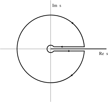
Figure 1: Integration contour in the $s=-Q^{2}$ plane, showing how analyticity is used to replace an integral along the cut by that along a circle. For the decay of the $\tau$ lepton (see section 3), the radius is equal to its mass $m_{\tau}$ squared.

This, however, poses a new problem, that of finding conditions under which an expansion of the type

$$f(1/Q^{2})\approx\sum_{k}a_{k}(q)/Q^{2k}$$ (5)

can be extended to the complex $Q^{2}$ plane, to be valid along all rays $|Q^{2}|\rightarrow\infty$. Such an extension is a delicate problem requiring precise mathematical conditions, which are not known in the case of QCD. To make the problem well-defined, recourse to simplifying mathematical assumptions therefore seems necessary.

While Wilson’s operator product expansion is originally formulated in the Euclidean domain, its applications are mostly related to quantities of the Minkowski nature. Then, the assumption is usually adopted [10] that the “convergence properties” of the operator-product expansion away from the euclidean ray $Q^{2}>0$ are the same as those along it, except the points of the cut $Q^{2}<0$ (the Minkowski region). Simultaneously, it is assumed that the truncation error (caused by approximating the operator product by several terms of the expansion) is independent of the direction in the complex $Q^{2}$ plane (see Fig. 1).

We consider this assumption too a severe simplification, in addition technically motivated: indeed, it is hard to believe that the unknown discontinuity along the cut would have no influence on the behaviour of the function along rays that are near the cut.

In the present paper we therefore look for a model scheme that would not a priori exclude the possibility that the bound on the truncation error (assumed originally in euclidean region) becomes looser with increasing deflection from the positive real semiaxis. The program of the paper was sketched in our previous papers, see [11] and [12]: We discuss conditions under which an expansion of the type (5) can be extended to angles away from the euclidean semiaxis in the complex $Q^{2}$ plane, with the aim to find how a bound, originally assumed to be valid along the positive real semiaxis, develops when the deflection increases and the cut is approached. We propose (in section 2 of the present paper) a scheme that (i) has precise mathematical meaning, (ii) is free from the a priori assumption that the influence of the cut on the truncation error along a general ray can be neglected and, simultaneously, (iii) tries to keep the model possibly close to real situations. To illustrate the physical interest of such a problem, we discuss in section 3 the determination of the coupling constant from the $\tau$ lepton hadronic width. Our results are presented and discussed in section 4. In the concluding section 5 we summarize our results, and discuss several possibilities of refining the scheme to get closer to physical reality. The three Appendices contain the proof of the main theorem on which our results are based, and an example of a function that saturates the bound (40) obtained in the Appendix A.

2 The operator-product expansion away from
euclidean region

Let $F(s)$ be holomorphic in ${\cal C}$, the complex $s$ plane ($s=-Q^{2}$) cut along $s\,\in\,[0,\infty]$ from which a bounded domain around the origin may be removed. Let the constants $a_{k}$, $k=0,1,2,...n-1$, and a positive number $A_{n}$ exist such that the following inequality

$$|F(s)-\sum_{k=0}^{n-1}a_{k}/(-s)^{k}|<A_{n}/|s|^{n}$$ (6)

is satisfied for a positive integer $n$ and all $s<-b$, with $b$ being a positive number. (To avoid unnecessary complications, we take the lowest value of $k$ to be zero, assuming that terms that are infinite at $|s|=\infty$ have been removed.) The problem is what inequality (if any) will hold along rays in the complex $s$ plane, away from the negative real semiaxis (euclidean region).

As is natural to expect, the answer depends on additional assumptions imposed on the function $F(s)\equiv f(1/Q^{2})$. When compared with the problem of the operator-product expansion in QCD, we make the following extra assumptions:

1. The coefficient functions $a_{k}$ of local operators are perturbative series in powers of the QCD coupling constant $\alpha_{s}(Q^{2})$, which in turn is expanded in negative powers of $\ln(Q/\Lambda)$ with coefficient functions depending on $\ln\ln(Q/\Lambda),\ln\ln\ln(Q/\Lambda)$, etc. Here, $\Lambda$ is $\Lambda_{\rm QCD}$, the fundamental scale of quantum chromodynamics. It is sometimes instructive to consider the form of the power corrections in the case that the logarithmic $Q^{2}$-dependence of the coefficient functions is neglected. We make this approximation for simplicity in the present paper, with the aim to examine the general case in a later publication. (In this approximation, the cut due to the logarithmic dependence of the Wilson coefficients disappears, but $F(s)$ can still have a cut if the expansion has an infinite number of terms or if additional singular terms are added to the series, see below.)

2. We assume that the inequality (6) is valid up to $s=-\infty$ , where the right-hand side of (6) vanishes at a high rate. This amounts to assuming that the $n$-th order remainder $R_{n}(-1/s)$,

$$R_{n}(z)=f(z)-\sum_{k=0}^{n-1}a_{k}z^{k},$$ (7)

tends to zero for $z\rightarrow 0$ as the $n$-th power of $z$ for at least one value of $n$.

These two assumptions simplify our problem but they may move us farther from physics. We plan to refine the scheme in a subsequent paper; our principal intention here is to create a model which would be free from the conventional assumption that the truncation error is the same in all directions (except the cut).

In phenomenological applications, the starting estimate of the truncation error in euclidean region is usually taken to be of the order of the first neglected term of the expansion. This term serves as a pragmatic guidance in estimating the size of the error; then, its value is conventionally extended to be the estimate of the truncation error along all rays passing through the origin.

It is our aim to obtain a more realistic picture about how the error may develop when the cut is approached. We examine the high-energy properties of the expansion (5) along different rays in the complex plane. Assuming the bound (6) for $s<-b$, we observe how it varies with increasing deflection of the ray from euclidean region.

Note that we do not demand that the expansion (5) be convergent or asymptotic to the expanded function $f(1/Q^{2})$: our approach is more general and can be applied whenever the remainder $R_{n}(1/Q^{2})$ obeys (6) at least for one fixed value of $n$, i.e., tends to zero as $1/Q^{2n}$ or faster in the euclidean domain. This allows, under the conditions specified below, an analytic continuation of the truncation error from the euclidean to the Minkowski domain. If the starting inequality (6) is known for several values of $n$, one can perform the continuation for each of them, term by term.

Recent applications of the operator product expansion in QCD have focused on problems dealing with quantities that are essentially related to the Minkowski domain, where the properties of the OPE are least known and may be completely different from those in the Euclidean domain. Inclusive decays of heavy flavours have been discussed. The ’t Hooft model [13] of two-dimensional QCD in the limit of many colours has been considered, [14], with the aim to abstract general features that may survive in four-dimensional QCD. We refer the reader to the papers quoted for details. Here let us briefly discuss the example of the determination of $\alpha_{s}(m^{2}_{\tau})$ from the $\tau$ lepton hadronic width, to illustrate physical relevance of the problem.

3 Determination of $\alpha_{s}(m_{\tau}^{2})$ from the $\tau$ lepton hadronic width

The $\tau$ lepton occupies a special position among all leptons, being the only lepton heavy enough to decay into hadrons. The $\tau$ decay provides a unique chance to study hadronic weak interactions at moderate energies. There has been extensive interest in using measurements of its total hadronic decay width $R_{\tau}$ (normalized to the leptonic width),

$$R_{\tau}=\frac{\Gamma[\tau^{-}\rightarrow\nu_{\tau}+{\rm hadrons}]}{\Gamma[\tau^{-}\rightarrow\nu_{\tau}{\rm e}^{-}\bar{\nu}_{\rm e}]},$$ (8)

to extract the renormalized strong-coupling parameter $\alpha_{s}$. This quantity possesses a number of advantages compared with other QCD observables. It is expected to be calculable in QCD using analyticity and the operator product expansion. It is an inclusive quantity which has been calculated perturbatively to the order $O(\alpha_{s}^{3})$. The $\tau$ mass, big as it is, is nevertheless below the threshold for charmed hadron production.

Starting from analyticity and the operator product expansion Braaten, Narison and Pich [10] used the measurements of the $\tau$ decay rate to determine the QCD running coupling constant at the scale of the $\tau$ mass $m_{\tau}$. The ratio $R_{\tau}$ is represented in the form

$$12\pi\int_{0}^{m_{\tau}^{2}}(1-s/m_{\tau}^{2})^{2}(1+2s/m_{\tau}^{2}){\rm Im}\,\Pi(s)\frac{{\rm d}s}{m_{\tau}^{2}},$$ (9)

where $\Pi(s)$ is a combination of correlators $\Pi^{\mu,\nu}_{i,j,V}$, $\Pi^{\mu,\nu}_{i,j,A}$ corresponding to the two-point correlation functions for the vector $V_{ij}^{\mu}=\bar{\psi}_{j}\gamma^{\mu}\psi_{i}$ and axial vector $A_{ij}^{\mu}=\bar{\psi}_{j}\gamma^{\mu}\gamma_{5}\psi_{i}$ colour singlet massless quark currents, with coefficients given by the elements $V_{{\rm ud}}$ and $V_{{\rm us}}$ of the Kobayashi-Maskawa matrix, the subscripts $i,j=$u,d,s denoting light quark flavours. For instance,

$$\Pi^{\mu,\nu}_{i,j,V}(s)=i\int{\rm d}^{4}x\,e^{iq\cdot x}\,\langle 0|\,T\,\{V^{\mu}_{i,j}(x),V^{\nu}_{i,j}(0)^{\dagger}\}\,|0\rangle=(q^{\mu}q^{\nu}-g^{\mu\nu}q^{2})\,\Pi_{i,j,V}(s).$$ (10)

The integral (9) cannot at present be calculated from QCD, because the hadronic functions are sensitive to the non-perturbative effects confining quarks in hadrons. But one can make use of the analyticity property of the correlating functions in the complex $s$-plane cut along the positive real semiaxis. This allows one to express (9) as a contour integral along the circle of radius $m_{\tau}^{2}$:

$$6\pi{\rm i}\oint_{|s|=m_{\tau}^{2}}(1-s/m_{\tau}^{2})^{2}(1+2s/m_{\tau}^{2})\Pi(s)\frac{{\rm d}s}{m_{\tau}^{2}}$$ (11)

(see Fig. 1, showing how analyticity is used to obtain $R_{\tau}$ from (11)). While in (9) the integration path $0\leq s\leq m_{\tau}^{2}$ runs along the cut, the integration contour in (11) keeps distance from it (with the exception of one point, $s=m_{\tau}^{2}$, and its neighbourhood), thereby giving a justification for representing $\Pi(s)$ as the operator-product expansion over local operators (provided that the value of $m_{\tau}$ is large enough, see a discussion in [10]).

In an analogous way, other weighted integrals (moments) of ${\rm Im}\Pi(s)$,

$$R_{\tau,\,V/A}^{l,\,m}(s_{0})=\int_{0}^{s_{0}}{\rm d}s(1-s/s_{0})^{l}(s/m_{\tau}^{2})^{m}\,\,\frac{{\rm d}R_{\tau,\,V/A}^{l,\,m}}{{\rm d}s},$$ (12)

have approximately been calculated within the framework of QCD. These moments can also be expressed as contour integrals analogous to (11).

It is to be expected that the error brought about by truncating the operator-product expansion of $\Pi(s)$ will be larger along rays that are closer to the cut $s\geq 0$. There is in particular a special danger that the integral (11) receives essential contributions from an interval around $s=m_{\tau}^{2}$, where the OPE has little chance appropriately to represent the function expanded. A fortunate circumstance is that the double zero of the kinematic factor $(1-s/m^{2}_{\tau})^{2}$ in the integrand suppresses the contribution from this dangerous segment. But a quantitative analysis of this argument is, to the best of our knowledge, still lacking. Moreover, as is emphasized in [15], experimental data are, because of the same factor $(1-s/m^{2}_{\tau})^{2}$, very poor and statistically limited around this point. An explicit estimate of the error is therefore desirable.

It is our aim to develop a scheme allowing a quantitative analysis of this qualitative argument. The method of obtaining the value of $\alpha_{s}$ from $R_{\tau}$ was repeatedly criticised in the literature [5, 16] for various reasons, claiming that the theoretical uncertainty usually quoted is underestimated. Leaving aside uncertainties related to the truncation of the perturbation series, we focus on two aspects related to the truncation of the operator product expansion. These aspects are:

1. The integral in (11) is carried out along the circle $|s|=m_{\tau}^{2}$. When $\Pi(s)$ in the integrand is approximated by the truncated OPE series, how does the remainder depend on the direction of the ray in the complex $s$ plane? One rightly expects that the error will increase with $s$ getting closer to the cut. But the quantitative aspect of this statement is unclear. How reliable is the expansion at those points $|s|=m_{\tau}^{2}$ that are far from the euclidean interval, yet not quite close to the double zero at $s=m_{\tau}^{2}$ ?

2. The terms exponential in $(-s)^{1/2}/\Lambda$, possibly to be added to the operator product expansion, are small along the euclidean ray and invisible in the truncated series, but may become big when the ray in the $s$ plane approaches the cut in the Minkowski domain. How does the effect of such additional terms depend on the deflection from euclidean region?

In the subsequent sections, we discuss these problems by examining the mathematical model outlined in sec. 2. We find conditions for obtaining bounds on the truncation errors in the whole complex high-energy domain; it turns out that these bounds are larger (and die off slower) in the Minkowski domain than in the euclidean domain.

4 Results and discussion

According to the notation introduced in Sec. 2, $f(z)$ represents a function holomorphic in a disk centred at the origin of the complex $z$ plane cut along the negative real semiaxis.

We consider two generic assumption schemes:

Case I : Let us assume that $f(z)$ has the form of the generalized Stieltjes integral (see [17])

$$f(z)=\int_{0}^{\infty}\frac{\rho(t)}{1+zt}{\rm d}t$$ (13)

and that the moments

$$a_{k}=\int_{0}^{\infty}t^{k}\rho(t){\rm d}t$$ (14)

exist for $k=0,1,2,...,n-1$, with $n$ being a fixed positive integer and $\rho(t)$ a real-valued function. Then, assuming a bound on the remainder (7) in euclidean region, we obtain a bound along all rays (see the formulae (16) and (19)).

Case II : The integral representation (13) is not a dispersion relation, because the function $\rho(t)$ has to vanish very rapidly for the moments $a_{k}$ (14) to exist. Beside this, non-power-like terms added to the operator-product expansion may violate the conditions (13), (14). We therefore build in subsection 4.2 a framework for more general situations, assuming an overall constant bound on $R_{n}(z)$. Then, using (6) on $R_{n}(z)$ along the euclidean ray, we obtain an angle-dependent bound along all rays (see the formula (32) or (33)), and observe how it deteriorates when the ray deflects from euclidean to the Minkowski region. The result (32), (33) is based on Theorem A of Appendix A.

In either case, the bounds obtained cannot be improved unless the respective class of functions is reduced to a smaller one. We show this by giving examples of functions saturating them in subsection 4.1 and in the Appendix C respectively.

4.1 Case I : The remainder in the form of a Stieltjes integral

Let us first assume that (13) and (14) hold with $\rho(t)$ nonnegative for $t\geq 0$. The remainders

$$R_{k}(z)=(-z)^{k}\int_{0}^{\infty}\frac{\rho(t)}{1+zt}t^{k}{\rm d}t,$$ (15)

with $k=1,2,...,n-1$, are bounded, for $z$ approaching zero along the positive real semiaxis, by

$$|R_{k}(z)|=\tilde{a}_{k}(z)|z|^{k}\leq a_{k}|z|^{k},$$ (16)

where we use the notation

$$\tilde{a}_{k}(z)=\int_{0}^{\infty}\frac{\rho(t)}{|1+zt|}t^{k}{\rm d}t.$$ (17)

It is easily seen that the inequality (16) is valid also for $z$ approaching zero along any ray lying in the right half of the complex plane because $|R_{k}(z)|\leq\tilde{a}_{k}(z)|z|^{k}$ and $\tilde{a}_{k}(z)\leq a_{k}$ for Re$z>0$. This, however, is not the case for Re $z<0$, due to the presence of the cut in this halfplane. The following bound can be obtained for Re$z<0$. We have, denoting $z=r{\rm e}^{{\rm i}\varphi}$,

$$|1+zt|=(1+2rt\cos\varphi+r^{2}t^{2})^{1/2}.$$ (18)

Considered as a function of $t$ at $t>0$ and $\varphi$ fixed ($\pi/2\leq|\varphi|\leq\pi$), $1/|1+zt|$ has its maximum at $t=-\frac{1}{r}\cos\varphi$, where its value is $1/|\sin\varphi|$. In this way we obtain (16) and

$$|R_{k}(z)|\leq a_{k}\,|z|^{k}/|\sin\varphi|$$ (19)

for Re$\,z>0$ and Re $z<0$ respectively. Comparing (19) with (16), we see how the factor $1/|\sin\varphi|$ makes the estimate looser when the ray gets closer to the cut, i.e., when $\varphi\rightarrow\pm\pi$.

The estimates become worse if the discontinuity along the cut is not positive definite. The corresponding bounds can be obtained by replacing $\rho(t)$ with $|\rho(t)|$ in the derivation.

Better bounds on $|R_{k}(z)|$ than (16) and (19) cannot be obtained unless some special assumptions about $\rho(t)$ are made. To see this, choose $\rho(t)=\rho_{0}(t)$ such that $f(z)$ has a pole, $\rho_{0}(t)=c\delta(t-t_{0})$ with $c>0$ and $t_{0}>0$, in which case $f(z)=c/(1+zt_{0})$, $a_{k}=ct_{0}^{k}$, and $|R_{k}(z)|=c|z|^{k}t_{0}^{k}/|1+zt_{0}|^{k}$. While the bound (16) for Re$z>0$ is saturated for $t_{0}>0$ tending to zero, (19) for Re$z<0$ is saturated for $t_{0}=-\frac{1}{r}\cos\varphi$.

It is of interest to see how the bounds (16) and (19) on the truncation error may affect the accuracy of the determination of the generic contour integral (11). As was discussed above, (16) and (19) are not immediately applicable in QCD to estimate the truncation error, due to the simplifying assumptions of our model. But it is interesting to compare them with the conventional assumption that the error is constant in all directions of the complex $z$ plane, which is a cruder approximation. To see this let us examine how the factor $|\sin\varphi|^{-1}$ in (19) affects the estimate of the integrals of the form (11).

As we have neglected the logarithmic dependence of the coefficient functions, the integral (11) can be evaluated trivially using Cauchy’s residue theorem. Representing the integration variable $s$ in the form $s=m^{2}_{\tau}{\rm e}^{{\rm i}\chi}$, $\chi=\pi-\varphi$, and replacing the function $\Pi(s)$ by the bound (16), (19) on $R_{k}(z)$, we obtain the following bound on the integrated remainder:

$$a_{k}6\pi m_{\tau}^{-2k}\left(I_{{\rm Eu}}^{2,1}+I_{{\rm Msin}}^{2,1}\right),$$ (20)

where

$$I_{{\rm Eu}}^{l,m}=\int_{\pi/2}^{3\pi/2}{\rm d}\chi|1-{\rm e}^{{\rm i}\chi}|^{l}|1+2{\rm e}^{{\rm i}\chi}|^{m}$$ (21)

and

$$I_{{\rm Msin}}^{l,m}=\left(\int_{0}^{\pi/2}+\int_{3\pi/2}^{2\pi}\right){\rm d}\chi|1-{\rm e}^{{\rm i}\chi}|^{l}|1+2{\rm e}^{{\rm i}\chi}|^{m}/|\sin\chi|$$ (22)

corresponds to the euclidean and the minkowskian halfplane respectively.

The effect by which the discontinuity along the cut tells on the value of the truncation error can be seen when the sum

$$I_{2}^{l,m}=I_{{\rm Eu}}^{l,m}+I_{{\rm Msin}}^{l,m}$$ (23)

is compared with

$$I_{1}^{l,m}=I_{{\rm Eu}}^{l,m}+I_{{\rm Mi}}^{l,m},$$ (24)

where

$$I_{{\rm Mi}}^{l,m}=\left(\int_{0}^{\pi/2}+\int_{3\pi/2}^{2\pi}\right){\rm d}\chi|1-{\rm e}^{{\rm i}\chi}|^{l}|1+2{\rm e}^{{\rm i}\chi}|^{m},$$ (25)

in which the integrand does not contain the factor $1/|\sin\chi|$. The three integrals can be written in the form

$$I_{{\rm Eu}}^{l,m}=\int_{\pi/2}^{\pi}C^{l,m}(\chi)\,\,{\rm d}\chi,$$ (26)

$$I_{{\rm Msin}}^{l,m}=\int_{0}^{\pi/2}C^{l,m}(\chi)/\sin\chi\,\,{\rm d}\chi,$$ (27)

and

$$I_{{\rm Mi}}^{l,m}=\int_{0}^{\pi/2}C^{l,m}(\chi)\,\,{\rm d}\chi$$ (28)

respectively, where

$$C^{l,m}(\chi)=2^{l/2+m+1}(1-\cos\chi)^{l/2}(5/4+\cos\chi)^{m/2}.$$ (29)

We see that (20) is composed of two factors, $6\pi a_{k}m^{-2k}_{\tau}$ (which depends on the $k$-th moment $a_{k}$ and on the radius $m^{2}_{\tau}$ of the integration circle), and $I^{2,1}_{2}=I^{2,1}_{{\rm Eu}}+I^{2,1}_{{\rm Msin}}$ (which contains the factor $1/|\sin\chi|$). Certainly, $I_{{\rm Msin}}^{l,m}>I_{{\rm Mi}}^{l,m}$, which fact signals the zero of the denominator in (15). While $I_{2}^{0,1}$ is a divergent integral, $I_{2}^{1,1}$ turns out to be greater than $I_{1}^{1,1}$ by almost 24 per cent. This difference is 6.7 per cent for $(l,m)=(2,1)$ and further decreases with increasing $l$, but increases with increasing $m$ at fixed $l$. Details can be seen in Table 1.

$l\,\,\backslash\,\,m$	1	2	3	4
1	1.237	1.34	1.45	1.56
2	1.067	1.104	1.148	1.194
3	1.026	1.043	1.064	1.089
4	1.012	1.020	1.032	1.046

Table 1: The ratio $I^{l,m}_{2}/I^{l,m}_{1}$ for different values of $l$ and $m$. The ratio indicates how much the discontinuity along the cut affects the role of the truncation error in the integral $I_{2}^{l,m}$ when compared with $I^{l,m}_{1}$.

4.2 Case II : The remainder bounded by a constant

For functions $f(z)$ that do not satisfy the conditions of Case I, the following theorem may be useful.

Let ${\cal C}$ be the plane of complex numbers. Let ${\cal C}(d,\alpha)$, $0<\alpha\leq\pi$, be the open segment of angle $\alpha$, of the disk of radius $d>0$ centred at the origin. In other words, let ${\cal C}(d,\alpha)$ represent $z=r{\rm e}^{{\rm i}\phi},\,\,|\phi|<\alpha,\,\,0<r<d$ (see Fig. 2).

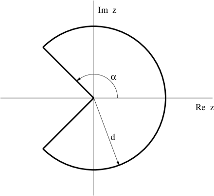
Figure 2: The region ${\cal C}(d,\alpha)$ in the complex $z$ plane. In this subsection, the case $\alpha=\pi$ is considered. See the Appendix for the general case.

Theorem 1. Let a function $f(z)$ be holomorphic in ${\cal C}(d,\pi)$. Let the remainder $R_{n}(z)$, see (7), fulfill, for a fixed positive integer $n$, the following two inequalities:

$$|R_{n}(z)|\leq M$$ (30)

for complex $z$, $z\in{\cal C}(d,\pi)$, and

$$|R_{n}(x)|\leq Ax^{n}$$ (31)

for $0<x<d$. Assume $d=\sqrt[n]{M/A}$. Then, for every $\varphi$, $|\varphi|<\pi$, $R_{n}(z)$ satisfies the inequality

$$|R_{n}(r{\rm e}^{{\rm i}\varphi})|\leq M^{1-\gamma}A^{\gamma}\,\,r^{\gamma n}$$ (32)

for all $z\in{\cal C}(d,\pi(1-\gamma))$, where and $\gamma=1-|\varphi|/\pi$.

This result is a special case of Theorem 2 (and Corollary 1), which is proved in the Appendix A. It gives an upper bound on $R_{n}(z)$ along every ray passing through the origin, the estimate becoming worse with increasing deflection from the positive real semiaxis, i.e., with the ray approaching the cut.

Remark 1. The equality $d=\sqrt[n]{M/A}$ is a special assumption saying that, for $z$ approaching the boundary point on the positive real semiaxis, $z=d$, the bounds (30) and (31) coincide. We make this assumption for simplicity of the subsequent discussion; see Appendix A for the general case.

Remark 2. The inequality (32) can also be written in the form

$$|R_{n}(r{\rm e}^{{\rm i}\varphi})|\leq M\,(r/d)^{\gamma n},$$ (33)

which reveals how the bound deteriorates with increasing distance from the origin and/or increasing angle (i.e., when energy decreases and, respectively, when the cut is approached; see a discussion below).

Remark 3. Compared with the conditions required in the previous subsection, no integral representations for $f(z)$ or the coefficients $a_{k}$ are required in the Theorem. On the other hand, by (30) a constant bound is imposed on $f(z)$ in ${\cal C}(d,\pi)$, which condition was not required in the Case I. In both cases, the resulting bound depends on the angle along which infinite energy is approached: In Case I, see (16) and (19), the coefficient is angle-dependent and the exponent $k$ is not, whereas in Case II, see (32) or (33), the exponent of $|z|$ is angle-dependent, decreasing from $n$ (along the positive real semiaxis) down to 0 (along the cut).

Remark 4. Since the resulting estimate (32) in ${\cal C}(d,\pi)$ is considerably looser than (31) for $0<x<d$ (note that the exponent is changed from $n$ in (31) to $\gamma n$ in (32), $0\leq\gamma\leq 1$, $\gamma$ tending to zero near the cut), it is interesting to look for a function that saturates it. A set of functions saturating (32) for different nonnegative integers $n$ can be generated by using the function $f(z)=\exp\{{\rm i}a\,\,[\,\ln(\sqrt{z}\,\,{\rm e}^{-{\rm i}\pi/2})\,]^{2}\}$ with $a$ real. This example (see the Appendix C for details) shows that the bounds are optimal, in the sense that they cannot be improved within the class of functions considered. There might be physical reasons, on the other hand, to restrict oneself to a smaller class of functions, in which case an improvement of the bound would be possible.

The resulting inequality (32) can be used to estimate, under the assumptions made, the error caused in (11) due to approximating $\Pi(s)$ in (11) by the first $n$ terms of the expansion. We observe the following facts:

1. To obtain a bound on the integral (11), we assume both (30) and (31). The inequality (31) alone (valid only in the euclidean region) is not sufficient for obtaining a bound on the remainder $R_{n}(z)$ at complex $z$, unless (30) is simultaneously used.

2. By Theorem 1, the bounds (30) and (31) are combined to create a third one, (32). While (30) is valid in the whole complex region ${\cal C}(d,\pi)$ but is loose, (31) holds only on the segment $0<x<d$ but is far more restrictive on this interval. Theorem 1 combines them to produce (32), which holds in ${\cal C}(d,\pi)$ and is restrictive, although less than (31), becoming (31) and (30) on the positive and the negative real semiaxis respectively. The resulting bound $M^{1-\gamma}A^{\gamma}\,r^{\gamma n}$ on the right hand side of (32) becomes (31) and (30) for $\gamma=1$ (euclidean region) and $\gamma$ approaching zero (minkowskian region) respectively.

3. For $r=d$, (32) is no improvement of (30). For $r<d$, (32) does imply an improvement of (30) thanks to (31), by means of the factor $(r/d)^{\gamma n}=r^{\gamma n}(A/M)^{\gamma}$ on the right hand side. This factor is smaller than 1 for $r<d$ and $|\varphi|<\pi$, but approaches 1 when $|\varphi|$ approaches $\pi$ at fixed $r$, or when $r$ approaches $d$ at fixed $\varphi$.

4. These results induce analogous relations between the corresponding integrals of the type (9), (11) and (12). Let us introduce the notation $\rho=r/d$. Inserting $M\rho^{n(1-|\varphi|/\pi)}$, the right-hand side of (32), into (11) instead of $\Pi(s)$, we find that the integral is bounded, due to (30), by

$$MI^{l,m}_{1}$$ (34)

while (32) imposes the bound

$$MJ^{l,m}(n,\rho)$$ (35)

with

$$J^{l,m}(n,\rho)=\int_{0}^{\pi}C^{l,m}(\chi)\,\,\rho^{n\chi/\pi}\,\,{\rm d}\chi.$$ (36)

on the same integral.

$n\,\,\backslash\,\,\rho$	0.05	0.2	0.4	0.6	0.8	0.9	1
1	0.18	0.38	0.57	0.73	0.87	0.936	1
2	0.051	0.17	0.34	0.54	0.76	0.87	1
3	0.020	0.081	0.21	0.40	0.66	0.82	1
4	0.009	0.044	0.13	0.30	0.58	0.77	1

Table 2: Thanks to (31), (30) improves into (32) and the corresponding integrated bound $MI^{l,m}_{1}$ into $MJ^{l,m}(n,\rho)$. The values of $J^{2,1}(n,\rho)/I^{2,1}_{1}$ shown in the table for different $n$ and $\rho$ illustrate the effect of Theorem 1 on the integrated bounds. Small values mean a big improvement, 1 means no improvement.

As we have seen, (31) can be used to improve the original bound (30) into (32). This induces an improvement of the bounds on the corresponding integrals, changing $MI^{l,m}_{1}$ into $MJ^{l,m}(n,\rho)$. The improvement is pronounced for small values of $\rho$ (which means that the disk ${\cal C}(d,\pi)$ is large), but becomes weak for $\rho$ approaching 1, when the boundary circle of ${\cal C}(d,\pi)$ is approached. The values of the ratio $J^{l,m}(n,\rho)/I^{l,m}_{1}$ for $(l,m)=(2,1)$ and some typical $n$ and $\rho$ are shown in Table 2.

It is difficult to make a straightforward comparison of the two bounds, (32) on one side and (16), (19) on the other, because they have been derived under different conditions. Perhaps the most striking difference is that, in Case I, $R_{k}(z)$ is holomorphic in the whole cut $z$ plane, while in Case II it is holomorphic only in the cut disk ${\cal C}(d,\pi)$; in this way, singularities of any kind are allowed outside ${\cal C}(d,\pi)$, arbitrarily near the boundary circle. The two assumption schemes therefore assign similar analyticity properties to $f(z)$ if the disk ${\cal C}(d,\pi)$ is very large, i.e., for small values of $\rho$ in (36).

$n\,\,\backslash\,\,\rho$	0.05	0.2	0.4	0.6	0.8	0.9	1
1	3.7	1.9	1.43	1.21	1.086	1.040	1
2	20	4.1	2.1	1.49	1.18	1.081	1
3	155	10	3.3	1.9	1.29	1.13	1
4	$10^{3}$	27	5.2	2.3	1.41	1.17	1

Table 3: When extrapolated into the cut disk, (31) deteriorates into (32) and the corresponding integrated bound $M\rho^{n}I^{l,m}_{1}$ into $MJ^{l,m}(n,\rho)$. The table shows the values of $J^{2,1}(n,\rho)/(\rho^{n}I^{2,1}_{1})$ for different $n$ and $\rho$. Large values, which signal a big deterioration (due to a strong angle dependence of (32)), appear near the origin (where $\rho$ is small) and/or at high expansion orders $n$.

The constant $M$ in (30) affects the value of the integral bound (35) in combination with the damping factor $\rho^{n\chi/\pi}$ in the integrand of (36), which becomes small when $n$ increases and/or $\rho$ decreases. It is instructive to compare the resulting bound $MJ^{l,m}(n,\rho)$ with that based on the assumption that (31) preserves its form in the whole cut disk. A convenient way to measure this effect is to divide $MJ^{l,m}(n,\rho)$ by $M\rho^{n}I^{l,m}_{1}$, in which the angle-dependent factor $\rho^{n\chi/\pi}$ in the integrand is suppressed, the exponent $n\chi/\pi$ being replaced by its value along the euclidean ray, $\chi=\pi$. By this, (31) is extended onto the whole cut disk. The resulting ratio is equal to $J^{l,m}(n,\rho)/(\rho^{n}I^{l,m}_{1})$; some numbers are given in Table 3 to illustrate the effect. While Table 2 shows what improvement of (30) is achieved thanks to (31) and the Theorem 1, Table 3 shows how strong the standard assumption of an overall validity of (31) is. Out of the three bounds, $M\rho^{n}I^{l,m}_{1}$ is the most restrictive one, while our result $MJ^{l,m}(n,\rho)$ based on the Theorem 1 is looser (as is shown in Table 3), and $M\,I_{1}^{l,m}$ based on (30) is the loosest (as is seen from Table 2). Thus,

$$M\,\rho^{n}\,I^{l,m}_{1}\leq M\,J^{l,m}(n,\rho)\leq M\,I_{1}^{l,m}.$$ (37)

The efficiency of our bound depends on the value of $\rho$, the ratio of $1/d$ (the lowest value of $|s|$ at which the bound (30) is supposed to hold) to $m_{\tau}^{2}$ (the radius of the integration contour of (11) in Fig. 1). Clearly, the problem has sense only for $\rho<1$, when the integration contour lies in the analyticity region. If the input bounds (30) and (31) are valid down to very low energies (i.e., if $1/d$ is small with respect to $m_{\tau}^{2}$), $\rho$ will be small and the right-hand side of (32) will become small as well, thanks to the factor $\rho^{n\chi/\pi}$. This improving factor is, however, strongly angle-dependent in the complex $s$ plane and will eventually, near the cut, rise to unity, thereby raising the bound (32) back to the starting inequality (30) at the points of the cut.

These results will be modified when the logarithmic dependence of the coefficient functions $a_{k}(q)$ is taken into account.

5 Concluding remarks

It has been our aim to propose a framework allowing a quantitative estimate of the truncation error of the operator-product expansion away from euclidean region. In considering the evaluation of the contour integrals of the type (9, 11) or (12), we have proposed two different sets of model assumptions to estimate the influence of the cut $s>0$ on the truncation error along different rays in the complex $s$ plane. In either case, the starting relation is the inequality (6) for negative $s$, $s<-b<0$. When combined with analyticity, (6) can be extended into the complex $s$ plane, but additional assumptions are necessary. We have cosidered two sets of them, (13), (14) (see Case I of section 4), and (30) (see Case II). The assumptions are rather strong in both cases, but are weaker than a straightforward extension of the inequality (6) into the $s$ plane. Also the resulting estimates ((16), (19) and, respectively, (32)) are considerably looser than such a straightforward extension. Some examples to illustrate this are in Table 3.

This result indicates, in view of the fact that our bounds can be saturated, that in applying an operator product expansion one should not mechanically extend (6) into the complex $s$ plane without special physical justification.

In either case, the resulting bounds exhibit a pronounced angle dependence in the $s$ plane, becoming worse and worse with increasing deflection from the euclidean region down to the cut. As a consequence, the integrated bounds on (9, 11) or (12) are looser than those based on the a priori assumption of angle independence. This result can be understood as a warning that conventional truncation error estimates used in phenomenology are perhaps too optimistic.

As our results are valid for certain classes of functions, a reduction of the class considered to a smaller one could yield a more restrictive upper bound. It is a challenge for physics to look for physically motivated class reductions.

Our results do not represent the complete solution to the problem. As mentioned in the Introduction, it was our aim to propose a model scheme that (i) would have precise mathematical meaning, (ii) would be free from the a priori assumption that the discontinuity along the cut has no influence on the truncation error along a general ray and, simultaneously, (iii) would keep the model possibly close to real situations. Whereas our model scheme satisfactorily meets the conditions (i) and (ii), it does not do full justice to the requirement (iii). We have made a step out of the schemes based on the a priori assumption that the truncation error is the same along all rays $|s|\rightarrow\infty$ passing through the origin. Our approach has been based on a plausible, but still crude picture of the operator product expansion. Further refinement is necessary. Next step should include allowance for the logarithmic $q$–dependence of the coefficients $a_{k}(q)$, and also a discussion of current QCD models [13], [14], [18]. An improvement of the integrated error estimate may be reached by introducing a subtracted dispersion relation and reversing the order of the $s$-integration and the $t$-integration (inclusive processes). Work along these lines is in progress.

Acknowledgements: We thank I. Caprini, E. de Rafael, A. Kataev, P. Kolář, V. Smirnov and J. Stern for stimulating discussions, and M. Flato for drawing our attention to Ref. [4]. One of us (J.F.) is indebted to A. de Rújula and the CERN Theory Division for hospitality. We acknowledge the support of the grants Nos. GAAV-A1010711, MSMT-VS96086, and GACR-202/96/1616.

Appendix A Appendix: Theorem A and its proof

Let ${\cal C}$ be the plane of complex numbers and ${\cal C}(d,\alpha)=\{z\in C:z=r{\rm e}^{{\rm i}\varphi},|\varphi|<\alpha,0<r<d\}$ where $d>0$ and $0<\alpha\leq\pi$ are given (see Fig 2).

Theorem 2. Let $f(z)$ be holomorphic in ${\cal C}(d,\alpha)$ and fulfilling

$$|f(z)|\leq M$$ (38)

for $z\in{\cal C}(d,\alpha)$ and

$$|f(x)|\leq Nx^{n}$$ (39)

for $0<x<d$, where $M$ and $N$ are positive constants. Denote $d_{0}=\sqrt[n]{M/N}$. Then

$$|f(z)|\leq|z|^{n/2}\sqrt{NM}$$ (40)

for $z\in{\cal C}(d,\alpha/2)$, $|z|\leq\min(d_{0},d)$ and

$$|f(z)|\leq M\,\,\,\,\,\,\,\,\,\,\,\,for\,\,z\in{\cal C}(d,\alpha/2),\,\,\,\,\,\,\,\,\,\,\min(d_{0},d)\leq|z|\leq d.\\$$ (41)

Remark 1. Repeating the statement of the Theorem we conclude that under the conditions of the Theorem we have: for every nonnegative integer $s$

$$|f(z)|\leq{\hat{N}}_{s}|z|^{n/2^{s}}$$ (42)

for $z\in{\cal C}(d,\alpha(1-2^{-s}))$, $|z|\leq\min(d_{0},d)$ and

$$|f(z)|\leq M\,\,\,\,\,\,\,\,\,\,\,\,for\,\,z\in{\cal C}(d,\alpha(1-2^{-s})),\,\,\,\,\,\,\,\,\,\,\min(d_{0},d)\leq|z|\leq d,\\$$ (43)

where

$${\hat{N}}_{s}=M(N/M)^{1/2^{s}}$$ (44)

is valid. This means that the remainder $R_{n}(z)$ (7) is bounded in the whole region ${\cal C}(d,\alpha)$ but the estimates are bad near the boundary.

Remark 2. By a reasoning similar to that used in the Proof of the Theorem the following statement can be proved. If a function $f(z)$ fulfils the assumptions of the Theorem, then

$$|f(z)|\leq{\tilde{N}}_{s}|z|^{n(1-2^{-s}})$$ (45)

for $z\in{\cal C}(d,\alpha/2^{s})$, $|z|\leq\min(d_{0},d)$ and

$$|f(z)|\leq M\,\,\,\,\,\,\,\,\,\,\,\,for\,\,z\in{\cal C}(d_{0},\alpha/2^{s}),\,\,\,\,\,\,\,\,\,\,\min(d_{0},d)\leq|z|\leq d.\\$$ (46)

is valid where

$${\tilde{N}}_{s}=M(N/M)^{1-1/2^{s}}.$$ (47)

This means that, in a small angle, the estimate can be improved.

Combining these two remarks we have

Corollary. If a function $f(z)$ fulfils the assumptions of the Theorem, then for every $\xi$, $0<\xi<1$, the following inequalities

$$|f(z)|\leq N_{\xi}|z|^{n(1-\xi)}\,\,\,\,\,\,for\,\,\,\,\,\,\,\,z\in{\cal C}(d,\alpha\xi),\,\,\,\,\,\,\,|z|\leq\min(d_{0},d)$$

$$|f(z)|\leq M\,\,\,\,\,\,\,\,\,\,\,\,for\,\,\,\,\,\,\,\,z\in{\cal C}(d,\alpha\xi),\,\,\,\,\,\,\,\,\,\,\min(d_{0},d)\leq|z|\leq d$$ (48)

are valid where

$$N_{\xi}=M(N/M)^{1-\xi}.$$ (49)

Proof of the Theorem. Denote

$$f_{1}(z)=\ln|f(z)|-\ln M.$$ (50)

The symbol $f_{1}(z)$ is understood as the harmonic function $f_{1}(x,y)$, where $z=x+{\rm i}y$. The symbol $f_{1}(x)$ is understood as $f_{1}(x,0)$. $f_{1}$ is a harmonic function in the region ${\cal C}(d,\alpha)-{\cal N}$ where ${\cal N}=\{z:f(z)=0\}$ is a countable set without condensation points in ${\cal C}(d,\alpha)$. The function $f_{1}(.)$ fulfils

$$f_{1}(x)\leq\min(n\ln x+\ln N-\ln M,0)$$ (51)

for real $x$ in $(0,d)-{\cal N}$. Further,

$$f_{1}(z)\leq 0$$ (52)

in ${\cal C}(d,\alpha)$ with the exception of countably many isolated points. Define

$$G(x)=\min(n\ln x+\ln N-\ln M,0).$$ (53)

The estimate $G(x)$ of $f_{1}(x)$ is nonpositive for $0<x\leq d$.

Now we introduce the notation ${\cal D}=\{z\in C:z=r{\rm e}^{{\rm i}\varphi},0<\varphi<\alpha,0<r<d\}$, and define the function $g_{1}(z)$ which is
(a) harmonic, nonpositive and maximal in the region ${\cal D}(d,\alpha)$ and continuously extensible on $\{x:0<x\leq d\}$, a part of the boundary of ${\cal D}(d,\alpha)$, with exception of countably many isolated points, and
(b) fulfilling

$$g_{1}(x)\leq G(x)\,\,\,\,\,\,\,\,{\it for}\,\,\,\,0<x\leq d.$$

Such function really exists (see Appendix B). It follows that the function fulfils

$$g_{1}(x)=G(x)\,\,\,\,\,\,for\,\,\,\,\,\,0<x\leq d,$$ (54)

$$g_{1}(x\exp({\rm i}\alpha))=0\,\,\,\,for\,\,\,\,0<x\leq d,$$

$$g_{1}(d\exp({\rm i}\varphi))=0\,\,\,\,\,for\,\,\,\,0\leq\varphi\leq\alpha.$$

In a similar way, we define a symmetric harmonic function $g_{2}(z)$ fulfilling (a) and the inequality

$$g_{2}(x{\rm e}^{{\rm i}\alpha})\leq G(x)\,\,\,\,for\,\,\,\,0<x\leq d$$

with exception of countably many isolated points. This function fulfils

$$g_{2}(x{\rm e}^{{\rm i}\alpha})=G(x)\,\,\,\,\,\,for\,\,\,0<x\leq d$$ (55)

$$g_{2}(x)=0\,\,\,\,\,\,for\,\,\,\,\,\,\,\,0<x\leq d$$

$$g_{2}(d{\rm e}^{{\rm i}\varphi})=0\,\,\,\,\,\,for\,\,\,\,0\leq\varphi\leq\alpha.$$

The sum $g(z)=g_{1}(z)+g_{2}(z)$ certainly fulfils the inequality (the $g_{i}$ are maximal)

$$g(z)\leq G(|z|)$$

so that the symmetry of the functions $g_{i}$ yields

$$g_{1}(x{\rm e}^{{\rm i}\alpha/2})=g_{2}(x{\rm e}^{{\rm i}\alpha/2})\leq G(x)/2.$$

If we compare the functions $f_{1}$ and $g_{1}$ we obtain (see Appendix B)

$$f_{1}(z)\leq g_{1}(z)\,\,\,\,\,\,in\,\,\,\,\,\,{\cal D}(d,\alpha)-{\cal N}.$$ (56)

We have

$$g_{1}(x{\rm e}^{{\rm i}\alpha/2})\leq G(x)/2.$$

Since $G(x)$ is nonpositive we have

$$g_{1}(x)\leq G(x)/2.$$

These conditions together with (56) and the maximality yields

$$f_{1}(z)\leq G(|z|)/2\,\,\,\,\,\,in\,\,\,\,\,\,{\cal D}(d,\alpha/2)$$

under the condition that we define $f_{1}(z)=-\infty$ for $z\in{\cal N}$. Using the definitions of the functions $f_{1}$ we obtain the statement of the Theorem.

Appendix B Appendix: Proof of two statements

(i) Proof of maximality. The region ${\cal D}(d,\alpha)$ can be conformally mapped on the unit disk. Denote $\Gamma$ and $\gamma(.)$ the image of the interval $(0,d]$ and the image of the function $G(x)$, respectively. Due to the theorem [19] (Chap. 3, page 33-34, item (v)) the maximal harmonic function fulfilling the condition (a) is given by the Poisson formula

$$\frac{1}{2\pi}\int_{\Gamma}\gamma(\psi)\frac{1-|z|^{2}}{1-2|z|\cos(\arg z-\psi)+|z|^{2}}{\rm d}\psi.$$

(ii) Proof of (56). Let $\{d_{n}\}$, $\{\alpha_{n}\}$ and $\{\rho_{n}\}$ be sequences fulfilling the inequalities $d_{n}<d$, $\alpha_{n}<\alpha$ and $\rho_{n}>0$ and converging to $d$, $\alpha$ and 0, respectively. Denote ${\cal D}_{n,m}={\cal D}(\rho_{m},d_{n},\alpha_{n})={\cal D}(d_{n},\alpha_{n})-{\cal D}(\rho_{m},\alpha_{n})$. Assume that the sequences are chosen so that $\partial{\cal D}_{n,m}\cap{\cal N}\subset(\rho_{m},d_{n}]$, where $\partial{\cal D}_{n,m}$ denotes the boundary of ${\cal D}_{n,m}$. This means that ${\cal D}_{n,m}$ contains only a finite number of points from ${\cal N}$. ${\cal D}_{n,m}$ can be conformally mapped on the unit disc (denoted by ${\cal U}$). Further denote $f^{n,m}$ and $h^{n,m}$ the image of $f_{1}$ and $f/M$ respectively. Then certainly $f^{n,m}=\ln|h^{n,m}|$. The function $h^{n,m}$ has only a finite number of zero points in ${\cal U}$. Let $\{z_{1},z_{2},...,z_{s}\}$ be the zero points with multiplicities $\{n_{1},n_{2},...,n_{s}\}$. Since $h_{n,m}/\Pi(z-z_{i})^{n_{i}}$ is a nonzero holomorphic function in ${\cal U}$ the function

$$F^{n,m}(z)=f^{n,m}(z)-\sum_{i=1}^{s}n_{i}\ln|\frac{z-z_{i}}{1-z\bar{z}_{i}}|$$ (57)

is a harmonic function in ${\cal U}$. Since the functions $\ln|(z-z_{i})/(1-z\bar{z}_{i})|$ vanish on $\partial{\cal U}$ and $f^{n,m}(z)$ are nonpositive, the functions $F^{n,m}(z)$ are nonpositive, too. Due to the theorem from [19] there exists a nonpositive measure $\mu$ on $\partial{\cal D}$ such that

$$F^{n,m}(z)=f^{n,m}(z)-\sum_{i=1}^{s}n_{i}\ln|\frac{z-z_{i}}{1-z\bar{z}_{i}}|=\frac{1}{2\pi}\int_{-\pi}^{\pi}\frac{1-|z|^{2}}{1-2|z|\cos(\arg z-\psi)+|z|^{2}}{\rm d}\mu(\psi).$$ (58)

Let $\Gamma^{n,m}$ and $\gamma^{n,m}$ be the image of the set $(\rho_{m},d_{n})$ and of the function $G(.)$, respectively. Using again the fact that the functions $\ln|(z-z_{i})/(1-z\bar{z}_{i})|$ are zero on $\partial{\cal U}$ we have $F^{n,m}(z)=f^{n,m}(z)\leq\gamma^{n,m}(z)$ on $\Gamma^{n,m}$ and

$$F^{n,m}(z)\leq\frac{1}{2\pi}\int_{\Gamma^{n,m}}\gamma^{n,m}(\psi)\frac{1-|z|^{2}}{1-2|z|\cos(\arg z-\psi)+|z|^{2}}{\rm d}\psi.$$ (59)

Since the functions $\ln|(z-z_{i})/(1-z\bar{z}_{i})|$, $k=1,2,...,s$, are nonpositive in ${\cal U}$ (with exception of the point $z_{i}$), we obtain

$$f^{n,m}(w)\leq q^{n,m}(w)$$ (60)

in ${\cal U}$, where the $q^{n,m}(w)$ are defined by the last integral. Denote $\beta^{n,m}$ the preimage of the function $q^{n,m}(w)$. Certainly we have

$$f_{1}(z)\leq\beta^{n,m}(z)\,\,\,\,\,\,\,\,for\,\,\,\,\,z\in{\cal D}_{n,m}.$$ (61)

Due to (i) the functions $\beta^{n,m}(.)$ fulfil the condition (a) of the Appendix A in the region ${\cal D}_{n,m}$ and the condition $\beta^{n,m}(x)\leq G(x)$ for $x\in(\rho_{m},d_{n}]$. Further, the functions $\beta^{n,m}(x)$ fulfil

$$\beta^{n,m}(x)=G(x)\,\,\,\,for\,\,\,\,\rho_{m}<x\leq d_{n},$$ (62)

$$\beta^{n,m}(x\exp[{\rm i}\alpha_{n}])=0\,\,\,\,for\,\,\,\,\rho_{m}<x\leq d_{n},$$

$$\beta^{n,m}(d_{n}\exp[{\rm i}\varphi])=0\,\,\,\,for\,\,\,\,0\leq\varphi\leq\alpha_{n},$$

$$\beta^{n,m}(\rho_{m}\exp[{\rm i}\varphi])=0\,\,\,\,for\,\,\,\,0\leq\varphi\leq\alpha_{n}.$$

Since the functions $\beta^{n,m}(.)$ are maximal they form a nonincreasing sequence for $m\rightarrow\infty$ and fixed $n$ in ${\cal D}(d_{n},\alpha_{n})$, and are bounded from below by the maximal function $\beta^{n}$ in ${\cal D}(d_{n},\alpha_{n})$, which fulfils (a) in ${\cal D}(d_{n},\alpha_{n})$ and $\beta^{n}(x)\leq G(x)$ for $x\in(0,d_{n}]$. Denote $\nu^{n}(z)=\inf_{m}\beta^{n,m}(z)$ with fixed $n$; $\nu^{n}(.)$ is a harmonic function in ${\cal D}(d_{n},\alpha_{n})$, and since $\beta^{n}(x)$ is maximal we have $\nu^{n}(z)=\beta^{n}(z)$. Certainly we have

$$f_{1}(z)\leq\beta^{n}(z)$$ (63)

for all $n$. This procedure can be repeated for $n\rightarrow\infty$ and the inequality (56) is proved.

Appendix C Appendix: A function saturating the bound (40)

The following example shows that the exponent in (40) cannot be improved.

Example. Let $f(.)$ be the function

$$f(z)=\exp\{{\rm i}a\,\,[\,\ln(\sqrt{z}\,\,{\rm e}^{-{\rm i}\pi/2})\,]^{2}\}$$ (64)

where $a$ is a positive constant. The function is holomorphic in $C(\infty,\pi)$ and is bounded in $C(1,\pi)$. The function $f(z)$ can be rewritten

$$f(z)=|\sqrt{z}\,\,|\,^{2a(\pi/2-\arg\sqrt{z})}\,\exp\{{\rm i}a\,[(\ln\sqrt{|z|}\,\,)^{2}-(\pi/2-\arg\sqrt{z}\,)^{2}]\}$$

such that

$$|f(z)|=|z|^{a(\pi-\arg z)/2}.$$

This yields that $f(x)=x^{a\pi/2}$ along the positive real axis and converges to zero as $|z|^{a(\pi-\alpha)/2}$ along the ray $R_{\alpha}=\{z:\arg z=\alpha,{\rm Re}z>0\}$. Compare this with Corollary.

References

- [1] K.G. Wilson, Phys.Rev. 179 (1969) 1499
- [2] W. Zimmermann: Local Operator Products and Renormalization in Quantum Field Theory, in: Lectures on Elementary Particles and Quantum Field Theory, 1970; Brandeis University Summer Institute in Theoretical Physics, Volume 1, pp. 395-589. The M.I.T. Press, 1970
-
[3]
K.G. Wilson and W. Zimmermann, Commun.Math.Phys. 24
(1972) 87
P. Otterson and W. Zimmermann, ibid. p. 107 -
[4]
S. Ferrara, R. Gatto and A.F. Grillo, Nucl.Phys.
34 (1971) 349
S. Ferrara and G. Rossi, J.Math.Phys. 13 (1972) 499 -
[5]
M.A. Shifman: Theory of pre-asymptotic effects in
weak inclusive decays, in: Proceedings of the Conference on
”Continuous Advances in QCD”, A.V. Smilga (Ed.), World Scientific
1994, 249
M. Shifman, Int.J.Mod.Phys. A 11 (1996) 3195 -
[6]
V.A. Smirnov, Commun.Math.Phys. 134 (1990) 109
V.A. Smirnov, Mod.Phys.Lett. A10 (1995) 1485 - [7] V.A. Smirnov: Renormalization and Asymptotic Expansions. 1991 Birkhauser Verlag Basel, Boston, Berlin
- [8] M. Beneke: Renormalons, CERN-TH/98-233, July 1998, hep-ph/9807443
- [9] M.A. Shifman, A.I. Vainshtein and V.I. Zakharov, Nucl.Phys. B147 (1979) 385
-
[10]
E. Braaten, S. Narison and A. Pich, Nucl.Phys.
B 373 (1992) 581
A. Pich: QCD tests from tau decays. Invited talk at the 20th Johns Hopkins Workshop (Heidelberg, 27-29 June 1996), hep-ph/9701305 - [11] J. Fischer, Int.J.Mod.Phys. A 12 (1997) 3625
- [12] J. Fischer and I. Vrkoč: The operator-product expansion away from euclidean region, Nucl.Phys. B (Proc. Suppl.) 74 (1999) 337, hep-ph/9811293
- [13] G. ’t Hooft, Nucl.Phys. D75 (1974) 461
-
[14]
B. Chibisov, R.D. Dikeman, M. Shifman
and N.G. Uraltsev, Int.J.Mod.Phys. A 12 (1997) 2075
B. Grinstein and Richard F. Lebed, Phys.Rev D 57 (1998) 1366
B. Blok, M. Shifman and Da-Xing Zhang, Phys.Rev. D 57 (1998) 2691
I. Bigi, M. Shifman, N. Uraltsev and A. Vainshtein, Phys.Rev D 59 (1999) 054011 - [15] F. LeDiberder and A. Pich, Phys.Lett. B 289 (1992) 165
-
[16]
G. Altarelli, P. Nason and G. Ridolfi, Z.Phys. C 68
(1995) 257
P. Ball, M. Beneke and V.M. Braun, Nucl.Phys. B 452 (1995) 563
M. Neubert, Phys.Rev. D 51 (1995) 5924 - [17] Carl M. Bender and Steven A. Orszag: Advanced mathematical methods for scientists and engineers; McGraw-Hill Book Company, 1978, p. 121seq
- [18] S. Peris, M. Perrottet and E. de Rafael: Matching long and short distances in large- QCD. Preprint CPT-97/P.3638 and UAB-FT-443, hep-ph/9805442
- [19] K. Hoffman: Banach spaces of analytic functions. Prentice-Hall, INC, Englewood Cliffs, N.J., 1962.