Deep inelastic Scattering, QCD, and generalised vector dominance

Abstract

We provide a formulation of generalised vector dominance (GVD) for low–$x$ deep-inelastic scattering that explicitly incorporates the ${\gamma}^{\ast}\to q{\bar{q}}$ transition and a QCD-inspired ansatz for the $(q{\bar{q}})p$ forward-scattering amplitude. The destructive interference originally introduced in off-diagonal GVD is recovered in the present formulation and traced back to the generic structure of two-gluon-exchange as incorporated into the notion of colour transparency. Asymptotically, the transverse photoabsorption cross section behaves as $(\ln Q^{2})/Q^{2}$, implying a logarithmic violation of scaling for $F_{2}$, while the longitudinal-to-transverse ratio decreases as $1/\ln Q^{2}$.

I Introduction

The observation of diffractive production of high-mass states at HERA [1] at small values of the scaling variable $x\approx{Q}^{2}/{W}^{2}$ qualitatively confirms the expectation from generalised vector dominance (GVD) [2]. The starting point of GVD is provided by a mass dispersion relation, the spectral weight function therein containing the coupling of a vector state of mass $M_{V}$ to a timelike photon, as observed in ${e}^{+}\!{e}^{-}$ annihilation, and the forward scattering of the vector state from the nucleon.

Originating from the pre-QCD era, the coupling of the photon to the high-mass continuum of ${e}^{+}\!{e}^{-}$ annihilation is frequently described in a global effective manner; the $q{\bar{q}}$ jets originating from the ${\gamma}^{\ast}\!\to\!q{\bar{q}}$ coupling, as observed at sufficiently high energies in ${e}^{+}\!{e}^{-}$ annihilation, are not explicitly incorporated into the description [4] of deep inelastic scattering.

In the present work, we provide a formulation of GVD that quantitatively takes into account not only the energy dependence of the ${\gamma}^{\ast}{\to}q{\bar{q}}$ transition, but the dependence on the $q{\bar{q}}$ configuration as well within the spectral weight function of GVD. The ansatz for the subsequent scattering of the $q{\bar{q}}$ state will be inspired by QCD. The emphasis of the present work will be put on the general theoretical analysis. Even though numerical results will be given, it will not be the aim of the present work to carry out a detailed comparison with the experimental data.

In Sec. II, we formulate the virtual Compton forward amplitude in terms of the ${\gamma}^{\ast}\to q{\bar{q}}$ transition of a timelike photon, continued to the spacelike region via appropriate propagator factors, and an ansatz motivated by perturbative QCD (pQCD) for the $(q{\bar{q}})p$ forward scattering amplitude. The destructive interference originally incorporated into off-diagonal GVD [5] reappears as the essential feature of the pQCD-inspired ansatz.

In Sec. III, the results of Sec. II are rederived in transverse position space, using the notion of colour transparency.

In Sections IV and V, we explicitly present the consequences from the QCD-inspired GVD ansatz for the $Q^{2}$ dependence of the transverse and the longitudinal photon-absorption cross section.

Some conclusions are drawn in section VI.

II Off-diagonal Generalised Vector Dominance from QCD.

The GVD picture for the Compton forward amplitude is described in Fig.1. We start with the ${\gamma}^{\ast}{\to}q{\bar{q}}$ transition. We look at the transition of a timelike photon of mass ${q}^{2}{\equiv}{M}_{q{\bar{q}}}^{2}$ to the $q{\bar{q}}$ pair.

a)

b)

FIG. 1.: The Compton forward amplitude in the proton rest frame, a) in the Gedankenexperiment where a timelike photon of mass $q^{2}=M_{q{\bar{q}}}^{2}$ interacts with the nucleon, b) upon continuation from $q^{2}=M_{q{\bar{q}}}^{2}$ to $q^{2}=-Q^{2}<0$, with $x(\approx Q^{2}/W^{2}){\ll}~{}1$.

The four-momentum of the photon of mass ${q}^{2}{\equiv}{M}_{q{\bar{q}}}^{2}$ in its rest frame is given by ${q}^{\mu}={k}^{\mu}_{q}+{k}^{\mu}_{\bar{q}}=({M}_{q{\bar{q}}},{\vec{0}})$, where ${k}^{\mu}_{q}$ and ${k}^{\mu}_{\bar{q}}$ denote the four-momenta of the quark and antiquark, respectively.

The $q{\bar{q}}$ current may be written as

$${\bar{\it u}}^{(\lambda)}({k}_{q}){\gamma}^{\mu}{\it v}^{({\lambda}^{\prime})}({k}_{\bar{q}})=-{M}_{q{\bar{q}}}(0,\cos\vartheta\cos\varphi+{\rm i}\lambda\sin\varphi,\cos\vartheta\sin\varphi-{\rm i}\lambda\cos\varphi,-\sin\vartheta){\delta}_{\lambda,-{\lambda}^{\prime}}\ .$$ (1)

Here, $\vartheta$ and $\varphi$ denote the polar and azimuthal production angles of the quark with respect to the $z$–axis in the photon rest frame, ${\vec{k}}_{q}=|{\vec{k}}_{q}|\left(\sin\vartheta\cos\varphi,\sin\vartheta\sin\varphi,\cos\vartheta\right)$, ${\vec{k}}_{\perp}=|{\vec{k}}_{\perp}|\left(\cos\varphi,\sin\varphi\right)$, and $\lambda$, ${\lambda}^{\prime}$ denote twice the quark and antiquark helicities. The timelike photon is supposed to originate from the annihilation of an ${e}^{+}{e}^{-}$ pair, and the $z$–axis is chosen in the direction of the ${e}^{-}$ three-momentum in the ${e}^{+}{e}^{-}$ (photon) rest frame (cf. Fig.2.).

FIG. 2.: The process of ${e}^{+}{e}^{-}$ annihilation in the rest frame of the $q{\bar{q}}$ system.

The assumed origin of the timelike photon from ${e}^{+}{e}^{-}$ annihilation (obviously) not only defines the four-momentum, but the polarisation properties of the photon as well. Introducing longitudinal and transverse helicity states for the massive photon in its rest frame,

$${\epsilon}_{L}^{\mu}=(0,0,0,1),\quad{\epsilon}_{T}^{\mu}(\pm)=\frac{1}{\sqrt{2}}(0,1,\pm{\rm i},0),$$ (2)

one obtains

$${\it j}_{L} \equiv {\bar{\it u}}^{(\lambda)}({k}_{q}){\epsilon}_{{\mu}L}{\gamma}^{\mu}{\it v}^{({\lambda}^{\prime})}({k}_{\bar{q}})=-{M}_{q{\bar{q}}}\sin\vartheta{\delta}_{{\lambda},-{{\lambda}^{\prime}}}\ ,$$ (3)

$${\it j}_{T}(\pm) \equiv {\bar{\it u}}^{(\lambda)}({k}_{q}){\epsilon}_{{\mu}T}(\pm){\gamma}^{\mu}{\it v}^{({\lambda}^{\prime})}({k}_{\bar{q}})=\frac{{M}_{q{\bar{q}}}}{\sqrt{2}}e^{\pm{\rm i}\varphi}(\cos\vartheta\pm\lambda){\delta}_{\lambda,-{\lambda}^{\prime}}.$$ (4)

Substituting

$${\sin}^{2}\vartheta \equiv \frac{4{m}_{\perp}^{2}}{{M}^{2}_{q{\bar{q}}}}=4z(1-z)\ ,\quad\cos\vartheta=(2z-1)\ ,$$ (5)

where

$$z=\frac{1}{2}\pm\frac{1}{2}\sqrt{1-\frac{4{m}^{2}_{\perp}}{{M}^{2}_{q{\bar{q}}}}},\quad m_{\perp}^{2}\equiv k^{2}_{\perp},\quad(0~{}{\leq}~{}z~{}{\leq}~{}1)\ ,$$ (6)

one may represent (4) in a manifestly covariant form

$${\it j}_{L} = -{M}_{q{\bar{q}}}2\sqrt{z(1\!-\!z)}{\delta}_{{\lambda},-{\lambda}^{\prime}}\ ,$$ (7)

$${\it j}_{T}(\pm) = \frac{{M}_{q{\bar{q}}}}{\sqrt{2}}e^{\pm{\it i}\varphi}(2z-1\pm\lambda){\delta}_{{\lambda},-{\lambda}^{\prime}}\ .$$ (8)

Longitudinal and transverse components of the current are thus explicitly defined with respect to any Lorentz frame obtained from the rest frame by a Lorentz boost in the $z$ direction. In particular, when considering the forward amplitude for scattering of the $q{\bar{q}}$ state from the nucleon at high energies, an appropriate Lorentz boost in the $z$ direction is to be applied to the $q{\bar{q}}$ system. Incidentally, we note that $z$ from (6) can also be represented as

$$z=\frac{k^{0}+k^{3}}{q^{0}+q^{3}},\quad(k^{\mu}\equiv k_{q}^{\mu})\ .$$ (9)

Hence, $z$ is unchanged under Lorentz boosts along the photon direction. In the high-energy limit, $|q^{0}|\approx|q^{3}|\gg M_{q{\bar{q}}}$, $z$ becomes identical to the fraction of the longitudinal momentum [6] of the $q{\bar{q}}$ system carried by the quark $q$.

Since

$${M}^{2}_{q{\bar{q}}}=\frac{{k}_{\perp}^{2}}{z(1\!-\!z)}\ ,$$ (10)

we can, instead of the pair of variables $({M}_{q{\bar{q}}},z)$ characterising the $q{\bar{q}}$ state coupled to the timelike photon, alternatively use $(k^{2}_{\perp},z)$ in (8).

Relations (8), upon multiplication by the antiquark charge $(-e_{q})$, give the coupling to the (timelike) photon of the $q{\bar{q}}$ complex of mass ${M}_{q{\bar{q}}}$ (or, alternatively, the transverse momentum ${\vec{k}}_{\perp}$) and the additional “configuration” degree of freedom, $z$. Let us envisage a physical situation in which such a high-energy $q{\bar{q}}$ complex, originating from a timelike photon, hits the proton in its rest frame (Fig.1a). Continuing to spacelike four-momenta of the photon, $q^{2}{\equiv}-Q^{2}<0$, with $x\approx Q^{2}/W^{2}\ll 1$, requires multiplication of the $q{\bar{q}}$ forward scattering amplitude by the coupling to the photon from (8) and a propagator factor $1/(Q^{2}+M^{2}_{q{\bar{q}}})$.

At this point, the cases of transverse and longitudinal photons have to be discriminated. For transverse photons, one simply assumes that the dependence on $Q^{2}$ induced by the propagator is the only one in the high-energy limit with $x\approx Q^{2}/W^{2}\ll 1$. Accordingly,

$${\it A}_{{\gamma}^{\ast}p{\to}{\gamma}^{\ast}p}\sim{\overline{\cal M}}^{\ast}_{T}{\cal T}_{(q{\bar{q}})p\to(q{\bar{q}})p}{\overline{\cal M}}_{T}\ ,$$ (11)

where the $(q{\bar{q}})p$ forward scattering amplitude is denoted by ${\cal T}_{(q{\bar{q}})p\to(q{\bar{q}})p}$, and according to (8) and the above discussion

$${\overline{\cal M}}^{({\lambda},{\lambda}^{\prime})}_{T}({M}_{q{\bar{q}}},z,Q^{2})=-\frac{{e}_{q}}{Q^{2}+{M}_{q{\bar{q}}}^{2}}\frac{{M}_{q{\bar{q}}}}{\sqrt{2}}e^{\pm{\it i}\varphi}(2z-1\pm{\lambda}){\delta}_{\lambda,-{\lambda}^{\prime}}\ .$$ (12)

For longitudinal photons, the restriction that the photon couples to a conserved source leads to a $Q^{2}$ dependence in addition to the one induced by the propagator. Current conservation requires that the $q{\bar{q}}$ system couples to a conserved source. This leads [9] to an additional factor $\sqrt{Q^{2}/M^{2}_{q{\bar{q}}}}$. Even though this factor is related to the $(q{\bar{q}})p$ amplitude and not to the ${\gamma}^{\ast}~{}\to~{}q{\bar{q}}$ transition, it may be put together with the propagator to yield

$${\overline{\cal M}}^{({\lambda},{\lambda}^{\prime})}_{L}(M_{q{\bar{q}}},z,Q^{2})=-\frac{e_{q}}{Q^{2}+M_{q{\bar{q}}}^{2}}M_{q{\bar{q}}}\sqrt{\frac{Q^{2}}{M^{2}_{q{\bar{q}}}}}2\sqrt{z(1-z)}{\delta}_{\lambda,-{\lambda}^{\prime}}.$$ (13)

Inclusion of a quark mass, $m_{q}$, changes (10) to become $M^{2}_{q{\bar{q}}}=(k_{\perp}^{2}\!+\!m_{q}^{2})/(z(1-z))$. The transverse transition amplitude (12) is modified by an additive term proportional to $m_{q}$,

$${\overline{\cal M}}^{({\lambda},{\lambda}^{\prime})}_{T}({M}_{q{\bar{q}}},z,Q^{2})=-\frac{{e}_{q}}{(Q^{2}+M_{q{\bar{q}}}^{2})\sqrt{2}}\left[M_{q{\bar{q}}}e^{\pm{\rm i}\varphi}(2z-1\pm{\lambda}){\delta}_{\lambda,-{\lambda}^{\prime}}+\frac{(\lambda\pm 1)m_{q}}{\sqrt{z(1\!-\!z)}}{\delta}_{\lambda,\lambda^{\prime}}\right]\ ,$$ (14)

while the expression (13) for the longitudinal amplitude remains unchanged.

In terms of the imaginary part of the forward-scattering amplitude ${\cal T}$, the total photoabsorption cross section for transverse (${\gamma}^{\ast}_{T}$) and longitudinal (${\gamma}_{L}^{\ast}$) virtual photons, via the use of the optical theorem, becomes

$${\sigma}_{{\gamma}^{\ast}_{T,L}p}(W^{2},Q^{2})=\left[\frac{1}{2(2\pi)^{3}}\right]^{2}\sum_{\lambda,{\lambda}^{\prime}=\pm 1}\int dz\int d{z}^{\prime}\int_{|{\vec{k}}_{\perp}|\geq k_{\perp 0}}d^{2}{k}_{\perp}\int_{|{\vec{k}}_{\perp}^{\prime}|\geq k_{\perp 0}}d^{2}{k}_{\perp}^{\prime}\times$$ (16)

$${\cal M}^{(\lambda,\lambda^{\prime})}_{T,L}({\vec{k}}_{\perp}^{\prime},z^{\prime};Q^{2})^{\ast}{\cal T}_{(q{\bar{q}})p\to(q{\bar{q}})p}({\vec{k}}_{\perp}^{\prime},z^{\prime};{\vec{k}}_{\perp},z;W^{2}){\cal M}^{(\lambda,\lambda^{\prime})}_{T,L}({\vec{k}}_{\perp},z;Q^{2})\ ,$$

where

$${\cal M}^{(\lambda,\lambda^{\prime})}_{T,L}({\vec{k}}_{\perp},z;Q^{2})\equiv\frac{{\overline{\cal M}}^{(\lambda,\lambda^{\prime})}_{T,L}({\vec{k}}_{\perp},z;Q^{2})}{\sqrt{z(1-z)}}\ .$$ (17)

The overall factors $1/\sqrt{(z(1\!-\!z))}$ entering (16) via (17) originate from the phase–space factors $d^{3}{k}_{(i)}/(k^{0}_{(i)}2(2\pi)^{3})$. They were rewritten using the identities $d^{3}{k}_{(i)}/k^{0}_{(i)}\equiv d^{2}{k}_{\perp(i)}dk^{3}_{(i)}/k^{0}_{(i)}$ $=d^{2}{k}_{\perp(i)}dz_{i}/z_{i}$, where $z_{i}$ ($i=1,2$) is the fraction of the longitudinal $q{\bar{q}}$ momentum carried by one of the quarks ($z_{1}\!=\!z$, $z_{2}\!=\!1\!-\!z$).

In (16), we have indicated lower limits, $k_{\perp 0}$, for the integration over the transverse momenta. The lower limit in transverse-momentum space corresponds to a finite transverse extension of the $q{\bar{q}}$ state in position space (confinement). The threshold, $k_{\perp 0}$, is introduced, in order to allow (16) to be used in an effective description of ${\sigma}_{{\gamma}^{\ast}_{T,L}p}$ at low values of $Q^{2}$, where the low–lying vector mesons actually dominate the Compton forward amplitude.

So far, the $(q{\bar{q}})p$ scattering amplitude has been left unspecified. To proceed, we will look for guidance at the two-gluon-exchange [10] of perturbative QCD (pQCD). As illustrated in Fig. 3, two-gluon exchange contains “diagonal” as well as “off-diagonal” transitions with respect to the transverse momenta ${\vec{k}}_{\perp}$ and ${\vec{k}}_{\perp}+{\vec{l}}_{\perp}$ and the masses,

$$M^{2}_{q{\bar{q}}}=\frac{{\vec{k}}_{\perp}^{2}}{z(1-z)}\ ,\quad M^{\prime 2}_{q{\bar{q}}}=\frac{({\vec{k}}_{\perp}\!+\!{\vec{l}}_{\perp})^{2}}{z(1-z)}\ ,$$ (18)

of the incoming and outgoing $q{\bar{q}}$ state. Fermion (the quark $q$) and antifermion (the antiquark ${\bar{q}}$) couple with opposite sign to the gluon.

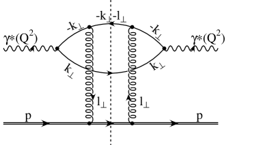
a)

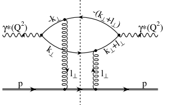
b)

FIG. 3.: The two-gluon exchange realisation of the structure (20), (24). The diagrams (a) and (b) correspond to transitions diagonal and off-diagonal in the masses of the $q{\bar{q}}$ pairs, respectively.

Accordingly, diagonal and off-diagonal transitions contribute with the same weight, but opposite signs. Guided by the structure of two-gluon exchange in pQCD, we adopt the following ansatz for the forward scattering amplitude in (16):

$${\cal T}_{(q{\bar{q}})p\to(q{\bar{q}})p}({\vec{k}}_{\perp}^{\prime},z^{\prime};{\vec{k}}_{\perp},z;W^{2})=$$ (20)

$$2(2\pi)^{3}\int d^{2}{l}_{\perp}{\tilde{\sigma}}_{(q{\bar{q}})p}(l^{2}_{\perp},W^{2})\left[\delta({\vec{k}}_{\perp}^{\prime}\!-\!{\vec{k}}_{\perp})\!-\!\delta({\vec{k}}_{\perp}^{\prime}\!-\!{\vec{k}}_{\perp}\!-\!{\vec{l}}_{\perp})\right]\delta(z\!-\!z^{\prime})\ ,$$

In addition to the difference in sign between the diagonal and the off-diagonal term, the ansatz (20) incorporates low–$x$ (high $W^{2}$) kinematics; the scattering is assumed to only affect the transverse momentum, while $z$ remains unchanged. Further, the $(q{\bar{q}})p$ interaction, ${\tilde{\sigma}}_{(q{\bar{q}})p}$, is assumed to solely be determined by the transverse momentum transfer $l^{2}_{\perp}$ and the c.m.s.–energy $W$.

Substituting (20) into (16) yields

$${\sigma}_{{\gamma}^{\ast}_{T,L}p} ( W^{2},Q^{2})=\frac{1}{16\pi^{3}}\sum_{\lambda,{\lambda}^{\prime}=\pm 1}\int dz\int d{z}^{\prime}\int d^{2}{l}_{\perp}{\tilde{\sigma}}_{(q{\bar{q}})p}(l^{2}_{\perp},W^{2})\int_{|{\vec{k}}_{\perp}|\geq k_{\perp 0}}d^{2}{k}_{\perp}\int_{|{\vec{k}}_{\perp}^{\prime}|\geq k_{\perp 0}}d^{2}{k}_{\perp}^{\prime}\times$$ (22)

$${\cal M}^{(\lambda,\lambda^{\prime})}_{T,L}({\vec{k}}_{\perp}^{\prime},z^{\prime};Q^{2})^{\ast}{\cal M}^{(\lambda,\lambda^{\prime})}_{T,L}({\vec{k}}_{\perp},z;Q^{2})\left[\delta({\vec{k}}_{\perp}^{\prime}\!-\!{\vec{k}}_{\perp})\!-\!\delta({\vec{k}}_{\perp}^{\prime}\!-\!{\vec{k}}_{\perp}\!-\!{\vec{l}}_{\perp})\right]\delta(z\!-\!z^{\prime})\ .$$

Upon integration over $d^{2}{k}_{\perp}^{\prime}$ and $d{z}^{\prime}$ (22) becomes

$${\sigma}_{{\gamma}^{\ast}_{T,L}p} ( W^{2},Q^{2})=\frac{1}{16\pi^{3}}\int dz\int d^{2}{l}_{\perp}{\tilde{\sigma}}_{(q{\bar{q}})p}({l}^{2}_{\perp};W^{2}){\Bigg{\{}}\int_{|{\vec{k}}_{\perp}|\geq k_{\perp 0}}d^{2}{k}_{\perp}\sum_{\lambda,{\lambda}^{\prime}=\pm 1}\left|{\cal M}^{(\lambda,{\lambda}^{\prime})}_{T,L}(z,{\vec{k}}_{\perp};Q^{2})\right|^{2}$$ (24)

$$-\int_{|{\vec{k}}_{\perp}|\geq k_{\perp 0},|{\vec{k}}_{\perp}\!+\!{\vec{l}}_{\perp}|\geq k_{\perp 0}}d^{2}{k}_{\perp}\sum_{\lambda,{\lambda}^{\prime}=\pm 1}{\cal M}^{(\lambda,{\lambda}^{\prime})}_{T,L}(z,{\vec{k}}_{\perp};Q^{2}){\cal M}^{(\lambda,{\lambda}^{\prime})}_{T,L}(z,{\vec{k}}_{\perp}\!+\!{\vec{l}}_{\perp};Q^{2})^{\ast}{\Bigg{\}}}\ .$$

The remarkable difference in sign between the diagonal and the off-diagonal term in (22) and (24), abstracted from perturbative QCD, actually implies significant cancellations between the contributions of the two terms. The first term under the integral in the curly bracket of (24) is related to the square of the amplitude of the process $({\gamma}^{\ast}\to q{\bar{q}})p\to{\rm hadrons}$ for fixed mass $M_{q{\bar{q}}}$ (cf. (10)), while the second term, the “off-diagonal” one with the negative sign in front, contains the product of the amplitudes for different masses, $M_{q{\bar{q}}}$ and $M^{\prime}_{q{\bar{q}}}$ (cf. (18)). It is worth noting that a structure of destructive interference between contributions diagonal and off-diagonal in the $q{\bar{q}}$ mass, as in (24), was actually suggested [5] a long time ago, in order to reconcile scaling in $e^{+}e^{-}$ annihilation with scaling in the deep inelastic scattering in conjunction with a reasonable (hadronic) cross section for the scattering of $q{\bar{q}}$–vector–meson states on the proton. In the framework of the off-diagonal generalised vector dominance model [5], the destructive interference was associated with the couplings of the photon to massive $q{\bar{q}}$–vector–meson states. Within the present pQCD-motivated ansatz (20), the destructive interference from off-diagonal GVD is recovered and traced back to the opposite couplings of the gluon to the quark and the antiquark the virtual photon has dissociated into.

III Position-space formulation, colour transparency.

In this Section, we rederive (22) in a position-space formulation. As the concept of “colour transparency” [10, 13] underlying the position-space formulation may also be motivated by the two-gluon exchange of perturbative QCD and its generalisation, it will come as no surprise that (22) will be recovered from an ansatz in position space.

We start by introducing the transverse position variable ${\vec{r}}_{\perp}$, conjugate to ${\vec{k}}_{\perp}$, by forming the Fourier transform of ${\cal M}^{(\lambda,{\lambda}^{\prime})}_{T,L}(z,{\vec{k}}_{\perp};Q^{2})$ from (17),

$${\psi}_{T,L}^{(\lambda,{\lambda}^{\prime})}(z,{\vec{r}}_{\perp};Q^{2}){\equiv}\frac{\sqrt{4\pi}}{16{\pi}^{3}}\int_{k_{\perp 0}}\!d^{2}{k}_{\perp}\exp{({\rm i}{\vec{k}}_{\perp}\cdot{\vec{r}}_{\perp})}{\cal M}^{(\lambda,{\lambda}^{\prime})}_{T,L}(z,{\vec{k}}_{\perp};Q^{2})\ .$$ (25)

The function ${\psi}_{T,L}^{(\lambda,{\lambda}^{\prime})}(z,{\vec{r}}_{\perp};Q^{2})$ [6] has frequently been called the “photon–$q{\bar{q}}$ wave function” [13].

The $\delta$–function dependence on the initial and final transverse momenta ${\vec{k}}_{\perp}$ and ${\vec{k}}^{\prime}_{\perp}$ in (22) suggests to adopt a representation for ${\sigma}_{{\gamma}^{\ast}_{T,L}p}$ in transverse position space that is diagonal with respect to ${\vec{r}}_{\perp}$,

$${\sigma}_{{\gamma}^{\ast}_{T,L}p}(W^{2},Q^{2})=\sum_{\lambda,{\lambda}^{\prime}=\pm 1}\int dz\int d^{2}{r}_{\perp}\left|\psi_{T,L}^{(\lambda,{\lambda}^{\prime})}(z,{\vec{r}}_{\perp};Q^{2})\right|^{2}{\sigma}_{(q{\bar{q}})p}({r}^{2}_{\perp},W^{2})\ ,$$ (26)

i.e. the cross section ${\sigma}_{{\gamma}^{\ast}_{T,L}p}$ is built up by multiplying the “dipole cross section” [13] ${\sigma}_{(q{\bar{q}})p}(r^{2}_{\perp},W^{2})$ by the probability to find the incoming quark and the incoming antiquark a transverse distance $r_{\perp}$ apart from each other. The longitudinal variable $z$ is “frozen” during the scattering process.

In a further step, we specify the relation between the dipole cross section (in position space) and the transverse-momentum-transfer function ${\tilde{\sigma}}_{(q{\bar{q}})p}(l^{2}_{\perp},W^{2})$ in (22). Requiring the dipole cross section to vanish for zero separation of quark and antiquark, as suggested by two-gluon exchange or by colour-neutrality of the $q{\bar{q}}$ state, we have

$${\sigma}_{(q{\bar{q}})p}({r}_{\perp}^{2},W^{2})=\int\!d^{2}{l}_{\perp}{\tilde{\sigma}}_{(q{\bar{q}})p}({l}_{\perp}^{2},W^{2})\left(1-{e}^{-{\rm i}{\vec{l}}_{\perp}\cdot{\vec{r}}_{\perp}}\right).$$ (27)

This ansatz indeed incorporates the required vanishing (colour tansparency [10, 13]), as $r_{\perp}^{2}$, for zero separation of quark and antiquark, $r_{\perp}\to 0$,

$${\sigma}_{(q{\bar{q}})p}({r}_{\perp}^{2},W^{2}) \to 0\qquad({\rm for}\ {r}_{\perp}\to 0)\ ,$$ (28)

as well as a constant limit for $r_{\perp}\to\infty$

$${\sigma}_{(q{\bar{q}})p}({r}_{\perp}^{2},W^{2}) \to {\sigma}^{(\infty)}_{(q{\bar{q}})p}(W^{2})\equiv\ {\sigma}^{(\infty)}_{(q{\bar{q}})p}\quad({\rm for}\ r_{\perp}\to\infty)\ ,$$ (29)

as the integral over the momentum space function has to be finite. From Fourier inversion of (27),

$${\tilde{\sigma}}_{(q{\bar{q}})p}({l}_{\perp}^{2},W^{2})=\frac{1}{{(2\pi)}^{2}}\int\!d^{2}{r}_{\perp}{e}^{{\rm i}{\vec{l}}_{\perp}\cdot{\vec{r}}_{\perp}}\left[{\sigma}_{(q{\bar{q}})p}^{(\infty)}-{\sigma}_{(q{\bar{q}})p}({r}_{\perp}^{2},W^{2})\right]$$ (30)

as well as from (29), we have ${\tilde{\sigma}}_{(q{\bar{q}})p}({l}^{2}_{\perp})\to 0$ for $l_{\perp}\to\infty$. Compare Figs. 4a, b for a sketch of the qualitative behaviour of ${\sigma}_{(q{\bar{q}})p}({r}_{\perp}^{2},W^{2})$ for two different simple choices of ${\tilde{\sigma}}_{(q{\bar{q}})p}({l}_{\perp}^{2},W^{2})$.

Inserting the dipole cross section (27), the position-space representation (26) for ${\sigma}_{{\gamma}^{\ast}_{T,L}p}(r^{2}_{\perp},W^{2})$ becomes

$${\sigma}_{{\gamma}^{\ast}_{T,L}p}(W^{2},Q^{2})=$$ (32)

$$\sum_{\lambda,{\lambda}^{\prime}=\pm 1}\int dz\int d^{2}{l}_{\perp}{\tilde{\sigma}}_{(q{\bar{q}})p}({l}^{2}_{\perp},W^{2})\int d^{2}{r}_{\perp}\left|\psi_{T,L}^{(\lambda,{\lambda}^{\prime})}(z,{\vec{r}}_{\perp};Q^{2})\right|^{2}\left(1-e^{-{\rm i}{\vec{l}}_{\perp}\!\cdot{\vec{r}}_{\perp}}\right)\ .$$

Upon introducing the ${\gamma}^{\ast}\to q{\bar{q}}$ transition amplitude (25), and integrating over position space, we have

$${\sigma}_{{\gamma}^{\ast}_{T,L}p} ( W^{2},Q^{2})=\frac{1}{16\pi^{3}}\sum_{\lambda,{\lambda}^{\prime}=\pm 1}\int dz\int d^{2}{l}_{\perp}{\tilde{\sigma}}_{(q{\bar{q}})p}({l}^{2}_{\perp},W^{2})\int_{|{\vec{k}}_{\perp}|\geq k_{\perp 0}}d^{2}{k}_{\perp}\int_{|{\vec{k}}_{\perp}^{\prime}|\geq k_{\perp 0}}d^{2}{k}_{\perp}^{\prime}\times$$ (34)

$${\cal M}_{T,L}^{(\lambda,{\lambda}^{\prime})}(z,{\vec{k}}_{\perp};Q^{2})^{\ast}{\cal M}_{T,L}^{(\lambda,{\lambda}^{\prime})}(z,{\vec{k}}_{\perp}^{\prime};Q^{2})\left[\delta({\vec{k}}_{\perp}^{\prime}\!-\!{\vec{k}}_{\perp})-\delta({\vec{k}}_{\perp}^{\prime}\!-\!{\vec{k}}_{\perp}\!-\!{\vec{l}}_{\perp})\right]\ .$$

This result for ${\sigma}_{{\gamma}^{\ast}_{T,L}p}$ indeed coincides with expression (22).

Similar forms of the dipole cross section ${\sigma}_{(q{\bar{q}})p}(r^{2}_{\perp})$ in (27) are obtained from a $\delta$–function ansatz and from a Gaussian ansatz for ${\tilde{\sigma}}_{(q{\bar{q}})p}({l}_{\perp}^{2})$ [cf. Figs. 4a, b],

$${\tilde{\sigma}}_{(q{\bar{q}})p}({l}_{\perp}^{2}) = \frac{{\sigma}_{(q{\bar{q}})p}^{(\infty)}}{\pi}\delta({l}_{\perp}^{2}-{\Lambda}^{2})\quad\Rightarrow\quad{\sigma}_{(q{\bar{q}})p}({r}^{2}_{\perp})={\sigma}_{(q{\bar{q}})p}^{(\infty)}\left(1-{J}_{0}({\Lambda}|{\vec{r}}_{\perp}|)\right)\ ;$$ (35)

$${\tilde{\sigma}}_{(q{\bar{q}})p}({l}_{\perp}^{2}) = \frac{{\sigma}_{(q{\bar{q}})p}^{(\infty)}}{\pi}{R}_{0}^{2}{e}^{-{l}_{\perp}^{2}R_{0}^{2}}\quad\Rightarrow\quad{\sigma}_{(q{\bar{q}})p}({r}_{\perp}^{2})={\sigma}_{(q{\bar{q}})p}^{(\infty)}\left(1-{e}^{-\frac{{r}_{\perp}^{2}}{4{R}_{0}^{2}}}\right)\ .$$ (36)

For simplicity of notation, in (35) and (36) the $W^{2}$–dependence of ${\tilde{\sigma}}_{(q{\bar{q}})p}(l^{2}_{\perp})$, ${\sigma}_{(q{\bar{q}})p}(r^{2}_{\perp})$ and ${\sigma}_{(q{\bar{q}})p}^{(\infty)}$ was dropped. From the subsequent examination of the transverse and the longitudinal cross section in (34), not unexpectedly, one finds that (35) and (36) lead to approximately the same results, provided one identifies the parameters $\Lambda$ and $R_{0}$ via $\Lambda=1/R_{0}$, where $R_{0}$ is of the order of the proton radius, $R_{0}\approx 1$ fm $\approx 0.2\ {\rm GeV}^{-1}$. We note that a Gaussian ansatz was employed in a recent analysis [14] of the experimental data. A different, polynomial representation for the $r_{\perp}^{2}$–dependence of the dipole cross section is used in Ref. [12].

FIG. 4.: The transverse-position-space dipole cross section ${\sigma}_{(q{\bar{q}})p}({r}^{2}_{\perp},W^{2})$ and its Fourier transform ${\tilde{\sigma}}_{(q{\bar{q}})p}({l}^{2}_{\perp},W^{2})$ for two simple choices in transverse momentum space, a) for a ${\delta}$–function and b) for a Gaussian.

IV Evaluation of ${\sigma}_{{\gamma}^{\ast}_{T,L}p}(W^{2},Q^{2})$, the explicit connection with off-diagonal generalised vector dominance.

The dependence of the ${\gamma}^{\ast}\!\to\!q{\bar{q}}$ transition amplitudes (12) and (13) on the propagator of the $q{\bar{q}}$ system of mass ${M}_{q{\bar{q}}}$ suggests a change of the integration variables in ${\sigma}_{{\gamma}_{T,L}^{\ast}p}$ in the expression (24). The angular integration over the direction of the transverse momentum of the incoming quark, ${\vec{k}}_{\perp}$, yields a factor $2\pi$, and we end up with

$$\int_{0}^{1}\!dz \int_{0}^{\infty}\!d^{2}{\vec{l}}_{\perp}\int_{k_{\perp 0}}^{\infty}\!d^{2}{\vec{k}}_{\perp}\ldots$$ (38)

$$={\pi}\int_{0}^{1}\!dzz(1\!-\!z)\!\int_{0}^{\infty}\!d{l}^{2}_{\perp}\int_{M_{0}^{2}(z)}^{\infty}\!dM^{2}\int_{(M-l_{\perp}^{\prime}(z))^{2}}^{(M+l_{\perp}^{\prime}(z))^{2}}\!dM^{\prime 2}w(M^{2},M^{\prime 2},{l}_{\perp}^{\prime 2}(z))\ldots\ ,$$

where

$$M_{0}^{2}(z)=\frac{k^{2}_{\perp 0}}{z(1-z)}\ .$$ (39)

In (38), we omitted the subscripts $q{\bar{q}}$ at the squared masses $M^{2}$ (10) and $M^{\prime 2}$ (18). The weight function $w(M^{2},M^{\prime 2},{l}_{\perp}^{2},z)$ appearing in (38) is given by

$$w(M^{2},M^{\prime 2},{l}_{\perp}^{\prime 2}(z))=\frac{1}{2M{M}^{\prime}\sqrt{1-\cos^{2}\phi}}\ .$$ (40)

The angle between ${\vec{k}}_{\perp}$ and ${\vec{k}}_{\perp}\!+\!{\vec{l}}_{\perp}$ has been denoted by $\phi$ (cf. Fig. 5) and $\cos^{2}\phi$, as a function of $M^{2}$, $M^{\prime 2}$, ${l}_{\perp}^{2}$ and $z$, is constrained by

$$\cos^{2}\phi\equiv\frac{1}{4M^{2}{M}^{\prime 2}}\left({M}^{2}\!+\!M^{\prime 2}\!-\!\frac{{l}_{\perp}^{2}}{z(1\!-\!z)}\right)^{2}\leq 1\ .$$ (41)

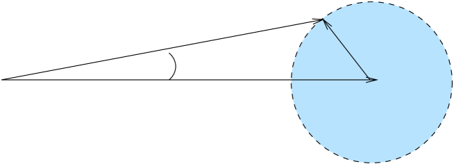
FIG. 5.: The pictorial expose of the quantities ${\vec{k}}_{\perp}$, ${\vec{l}}_{\perp}$, ${\vec{k}}_{\perp}+{\vec{l}}_{\perp}$, and the angle $\phi$.

This constraint implies bounds on the integration interval for the integration over $d{M}^{\prime 2}$. As indicated in (38), the bounds are given by ${(M\!\pm\!{l}^{\prime}_{\perp}(z))}^{2}$, where

$${l}^{\prime 2}_{\perp}\equiv{l}^{\prime 2}_{\perp}(z)=\frac{{l}^{2}_{\perp}}{z(1\!-\!z)}\ .$$ (42)

For later use we note

$$\int_{(M-{l}_{\perp}^{\prime}(z))^{2}}^{(M+{l}_{\perp}^{\prime}(z))^{2}}dM^{\prime 2}w(M^{2},M^{\prime 2},{l}_{\perp}^{\prime 2}(z))=\pi\ ,$$ (43)

as well as

$$\frac{\int_{(M-{l}_{\perp}^{\prime}(z))^{2}}^{(M+{l}_{\perp}^{\prime}(z))^{2}}dM^{\prime 2}w(M^{2},M^{\prime 2},{l}_{\perp}^{\prime 2}(z))M^{\prime 2}}{\int_{(M-{l}_{\perp}^{\prime}(z))^{2}}^{(M+{l}_{\perp}^{\prime}(z))^{2}}dM^{\prime 2}w(M^{2},M^{\prime 2},{l}_{\perp}^{\prime 2}(z))}=(M^{2}+{l}_{\perp}^{\prime 2}(z))\ .$$ (44)

In order to clarify the physical meaning of the right-hand side of (44), we observe that (24), upon removal of the $Q^{2}$–dependent propagator terms, becomes proportional to the purely hadronic cross section ${\tilde{\sigma}}_{(q{\bar{q}})p}$. Consequently, the quantity in (44) is the mean mass produced in the $(q{\bar{q}})p$ forward-scattering reaction at fixed values of $M$, $z$ and $l_{\perp}$.

In passing from the integration variables in (24) to the new ones introduced in (38), the integration limits on the integration over $dM^{\prime 2}$ and $dM^{2}$ have to be carefully looked at.

In the integration over $dM^{\prime 2}$, we first consider the first term in the curly brackets of (24), i.e., the term diagonal in the mass $M\!\equiv\!M_{q{\bar{q}}}$ of the $q{\bar{q}}$ pair. In this term, the integration over $dM^{\prime 2}$ [cf. (18)] corresponds to an integration over all directions of ${\vec{l}}_{\perp}$ in Fig. 5, i.e. to an integration over the range of $\phi$ allowed by (41) at fixed values of $M^{2}$, $l_{\perp}^{2}$ and $z$. The corresponding integration limits are as indicated in (38).

Concerning the second term, i.e. the off-diagonal one in the curly brackets of (24), we note that in this term integration over $dM^{\prime 2}$ describes integration over all final-state $q{\bar{q}}$ masses (18) in the Compton forward amplitude. For the off-diagonal term, consequently, the lower limit of integration in (38), namely $(M\!-\!l^{\prime}_{\perp}(z))^{2}$, must in addition be restricted to values above $M_{0}^{2}(z)$ from (39), as indicated in (24) already. After all, the photon couplings to the initial and final $q{\bar{q}}$ state in the Compton forward amplitude must be identical.

We turn to the integration over $dM^{2}$ in (38). In the diagonal term in (24), it describes integration over the ingoing and the outgoing mass, while in the off-diagonal term it describes integration over the mass of the incoming $q{\bar{q}}$ pair only. The necessity of a lower cutoff $M_{0}^{2}$ in the integration over $dM^{2}$ stems from the empirical fact that $e^{+}e^{-}\to{\gamma}^{\ast}\to q{\bar{q}}\to{\rm hadrons}$ becomes appreciable only when the centre-of-mass energy $\sqrt{s(e^{+}e^{-})}$ is above a lower threshold that depends on the flavour of the quark $q$. This suggests a limit of $M_{0}\leq M_{\rho}$, for $u$ and $d$ quarks, while $M_{0}\leq M_{J/{\Psi}}$ for the $c$ quarks, etc. Actually, in (38), we have indicated a $z$–dependent lower cutoff of $M_{0}^{2}(z)\!=\!k_{\perp 0}^{2}/(z(1\!-\!z))$. It originates from the lower bound on the transverse momentum of the quark $q$ in the incoming $q{\bar{q}}$ state as introduced in (25). While this $z$–dependent bound on squared masses $M^{2}_{q{\bar{q}}}$ is thus suggested by confinement, it should be kept in mind that the description of the coupling of the photon to the low–lying resonances in terms of a simple ${\gamma}^{\ast}\to q{\bar{q}}$ transition amplitude is an effective one [2] in the sense of averaging the total cross section over the contributing resonances, e.g., the $\rho^{0}$, $\rho^{\prime 0}$, etc. The $z$ dependence of the lower bound, $M_{0}^{2}(z)$, is accordingly to be looked at with some reservation. We will comment on the effect of the $z$ dependence of $M_{0}^{2}$ in the numerical analysis of Section V.

Returning to (24), inserting the expressions (12) and (13) for the ${\gamma}^{\ast}\to q{\bar{q}}$ transitions, and introducing the integration variables $M^{2}$ and $M^{\prime 2}$ according to (38), we get for the transverse photoabsorption cross section

$${\sigma}_{{\gamma}^{\ast}_{T}p}(W^{2},Q^{2})=\frac{\alpha}{2{\pi}}\left(\frac{e_{q}}{e_{0}}\right)^{2}\int_{0}^{\infty}d{l}^{2}_{\perp}{\tilde{\sigma}}_{(q{\bar{q}})p}\left({l}_{\perp}^{2},W^{2}\right)\int_{0}^{1}dz(1\!-\!2z(1\!-\!z))\times$$ (45)

$${\Bigg{\{}}\int_{M_{0}^{2}(z)}^{\infty}dM^{2}\int_{(M-{l}_{\perp}^{\prime}(z))^{2}}^{(M+{l}_{\perp}^{\prime}(z))^{2}}dM^{\prime 2}w(M^{2},M^{\prime 2},{l}_{\perp}^{\prime 2}(z))\left[\frac{M^{2}}{(Q^{2}+M^{2})^{2}}-\frac{M^{\prime 2}+M^{2}-{l}_{\perp}^{\prime 2}(z)}{2(Q^{2}+M^{2})(Q^{2}+{M}^{\prime 2})}\right]$$ (46)

$$+\int_{M_{0}^{2}(z)}^{\infty}\!\!dM^{2}\Theta(M_{0}^{2}(z)\!-\!(M\!-\!{l}_{\perp}^{\prime}(z))^{2})\times$$ (47)

$$\int_{(M\!-\!{l}_{\perp}^{\prime}(z))^{2}}^{M_{0}^{2}(z)}\!dM^{\prime 2}w(M^{2},M^{\prime 2},{l}_{\perp}^{\prime 2}(z))\frac{M^{\prime 2}\!+\!M^{2}\!-\!{l}_{\perp}^{\prime 2}(z)}{2(Q^{2}\!+\!M^{2})(Q^{2}\!+\!{M}^{\prime 2})}{\Bigg{\}}}\ ,$$ (48)

(49)

and for the longitudinal one

$${\sigma}_{{\gamma}^{\ast}_{L}p}(W^{2},Q^{2})=\frac{2\alpha}{{\pi}}\left(\frac{e_{q}}{e_{0}}\right)^{2}Q^{2}\int_{0}^{\infty}d{l}^{2}_{\perp}{\tilde{\sigma}}_{(q{\bar{q}})p}\left({l}_{\perp}^{2},W^{2}\right)\int_{0}^{1}dzz(1\!-\!z)\times$$ (50)

$${\Bigg{\{}}\int_{M_{0}^{2}(z)}^{\infty}dM^{2}\int_{(M-{l}_{\perp}^{\prime}(z))^{2}}^{(M+{l}_{\perp}^{\prime}(z))^{2}}dM^{\prime 2}w(M^{2},M^{\prime 2},{l}_{\perp}^{\prime 2}(z)){\Bigg{[}}\frac{1}{(Q^{2}+M^{2})^{2}}-\frac{1}{(Q^{2}+M^{2})(Q^{2}+{M}^{\prime 2})}{\Bigg{]}}$$ (51)

$$+\int_{M_{0}^{2}(z)}^{\infty}\!\!dM^{2}\Theta(M_{0}^{2}(z)\!-\!(M\!-\!{l}_{\perp}^{\prime}(z))^{2})\times$$ (52)

$$\int_{(M\!-\!{l}_{\perp}^{\prime}(z))^{2}}^{M_{0}^{2}(z)}\!dM^{\prime 2}w(M^{2},M^{\prime 2},{l}_{\perp}^{\prime 2}(z))\frac{1}{(Q^{2}\!+\!M^{2})(Q^{2}\!+\!{M}^{\prime 2})}{\Bigg{\}}}\ ,$$ (53)

where $\Theta(x)$ is the step function [$\Theta(x)\!=\!1$ for $x\!>\!0$, $\Theta(x)\!=\!0$ otherwise]. In (49) and (53), the $\Theta$–function term becomes unequal zero as soon as $(M\!-\!l_{\perp}^{\prime}(z))^{2}$ drops below $M_{0}^{2}(z)$, thus removing the above-mentioned forbidden region in the integration over $dM^{\prime 2}$ in the (main) off-diagonal term. We note that the “low-mass term” containing the $\Theta$–function is suppressed relative to the main off-diagonal term, as the intervals of the integration over $dM^{2}$ and $dM^{\prime 2}$ are very much restricted,

$$\int_{M_{0}^{2}(z)}^{\infty}\!dM^{2}\Theta\left(M_{0}^{2}(z)\!-\!(M\!-\!{l}_{\perp}^{\prime}(z))^{2}\right)\int_{(M\!-\!{l}_{\perp}^{\prime}(z))^{2}}^{M_{0}^{2}(z)}dM^{\prime 2}\ldots$$ (55)

$$=\int_{M_{0}^{2}(z)}^{(M_{0}(z)\!+\!{l}_{\perp}^{\prime}(z))^{2}}\!dM^{2}\!\int_{(M\!-\!{l}_{\perp}^{\prime}(z))^{2}}^{M_{0}^{2}(z)}\!dM^{\prime 2}\dots\ .$$

Actually, it will turn out that the main term in the transverse cross section will asymptotically behave like $(\ln Q^{2})/Q^{2}$, thus suppressing the ${\Theta}$–function term that behaves as $1/Q^{2}$. In the longitudinal cross section the suppression is less pronounced, as both the main term and the ${\Theta}$–function term behave as $1/Q^{2}$ for asymptotic $Q^{2}$. The subsequent analysis of this Section will be simplified by ignoring the ${\Theta}$–function terms in (49) and (53). We will come back to them, when turning to the numerical results in Section V.

In order to explicitly obtain the $Q^{2}$ dependence of ${\sigma}_{{\gamma}^{\ast}_{T}p}$ and ${\sigma}_{{\gamma}^{\ast}_{L}p}$ contained in (49) and (53), we proceed in several steps. In a first step, we will show that the transverse cross section (49) may be evaluated analytically in the limit of $Q^{2}\to\infty$ for the simple case of the $\delta$–function ansatz (35) for ${\tilde{\sigma}}_{(q{\bar{q}})p}(l^{2}_{\perp},W^{2})$. In the second step, we introduce mean values for the configuration variable, $z$, and for $M^{\prime 2}$ at fixed $M^{2}$ and $l^{2}_{\perp}=\Lambda^{2}$, and apply the mean-value theorem to the integration over $z$ and $M^{\prime 2}$ in the transverse cross section (49) for arbitrary values of $Q^{2}$. A similar procedure will be carried out for the longitudinal cross section. After these steps, the connection with the original formulation of off-diagonal GVD [5] will become explicit. The determination of the numerical values of the mean configuration variables, ${\bar{z}}_{T,L}$, and of the parameters $\delta_{T,L}$ characterising the mean mass, $M^{\prime}$, will be shifted to Section V.

A The transverse cross section, ${\sigma}_{{\gamma}^{\ast}_{T}p}$.

As noted, we ignore the ${\Theta}$–function term in (49), insert the $\delta$–function ansatz (35) for ${\tilde{\sigma}}_{q{\bar{q}}p}$, and carry out the integrations over $dl_{\perp}^{2}$ and $dM^{\prime 2}$, to obtain

$${\sigma}_{{\gamma}^{\ast}_{T}p} ( W^{2},Q^{2})=\frac{\alpha}{2{\pi}}\left(\frac{e_{q}}{e_{0}}\right)^{2}{\sigma}^{(\infty)}_{(q{\bar{q}})p}\int_{0}^{1}dz(1\!-\!2z(1\!-\!z))\int_{M_{0}^{2}(z)}^{\infty}dM^{2}\times$$ (57)

$$\left[\frac{M^{2}}{(Q^{2}+M^{2})^{2}}-\frac{1}{(Q^{2}+M^{2})}\frac{1}{2}\left(1+\frac{M^{2}-Q^{2}-{\Lambda}^{\prime 2}}{\sqrt{(Q^{2}+M^{2}+{\Lambda}^{\prime 2})^{2}-4{\Lambda}^{\prime 2}M^{2}}}\right)\right]\ ,$$

where ${\Lambda}^{\prime 2}\!\equiv\!{\Lambda}^{2}/(z(1\!-\!z))$. Replacing $z$ by the variable $u\equiv z(1-z)$ yields

$${\sigma}_{{\gamma}^{\ast}_{T}p} ( W^{2},Q^{2})=\frac{{\alpha}}{\pi}\left(\frac{e_{q}}{e_{0}}\right)^{2}{\sigma}^{(\infty)}_{(q{\bar{q}})p}\int_{0}^{1/4}du\frac{1-2u}{\sqrt{1-4u}}\int_{M_{0}^{2}(u)}^{\infty}dM^{2}\times$$ (59)

$$\left[\frac{M^{2}}{(Q^{2}+M^{2})^{2}}-\frac{1}{(Q^{2}+M^{2})}\frac{1}{2}\left(1+\frac{u(M^{2}-Q^{2})-{\Lambda}^{2}}{\sqrt{(u(Q^{2}+M^{2})+{\Lambda}^{2})^{2}-4u{\Lambda}^{2}M^{2}}}\right)\right]\ .$$

Expansion of the off-diagonal term in a power series for large $Q^{2}$ gives

$${\sigma}_{{\gamma}^{\ast}_{T}p}(W^{2},Q^{2})=\frac{{\alpha}}{\pi}\left(\frac{e_{q}}{e_{0}}\right)^{2}{\sigma}^{(\infty)}_{(q{\bar{q}})p}\int_{0}^{1/4}du\frac{1-2u}{\sqrt{1-4u}}\int_{M_{0}^{2}(u)}^{\infty}dM^{2}\frac{\Lambda^{2}}{(Q^{2}+M^{2})(u(Q^{2}\!+\!M^{2})+\Lambda^{2})}\times$$ (60)

$$\left[\frac{M^{2}}{(Q^{2}+M^{2})}+\frac{uM^{2}}{(u(Q^{2}\!+\!M^{2})+\Lambda^{2})}-\frac{2u^{2}M^{4}}{(u(Q^{2}\!+\!M^{2})+\Lambda^{2})^{2}}+\cdots\right]\ .$$ (61)

The integration over $dM^{2}$ and $du$ in (61) may now be carried out by expanding $1/\sqrt{1\!-\!4u}$ in powers of $u$ and integrating term by term. It turns out that the replacement of $1/\sqrt{1\!-\!4u}$ by $1\!+\!2u$ is sufficient to yield the leading term in the large–$Q^{2}$ limit of $Q^{2}\!\gg\!{\Lambda}^{2}$,

$${\sigma}_{{\gamma}^{\ast}_{T}p}(W^{2},Q^{2})=\frac{{\alpha}}{3\pi}\left(\frac{e_{q}}{e_{0}}\right)^{2}{\sigma}^{(\infty)}_{(q{\bar{q}})p}\left[\frac{{\Lambda}^{2}}{Q^{2}}\ln\left(\frac{Q^{2}}{{\Lambda}^{2}}\right)+c\frac{\Lambda^{2}}{Q^{2}}+{\cal O}\left(\frac{\ln Q^{2}}{Q^{4}}\right)\right]\ .$$ (62)

We note that the leading term in (62) is independent of the threshold mass parameterised by $k_{\perp 0}^{2}$. Moreover, (62) shows a logarithmic violation of scaling of the transverse part of the structure function $F_{2}\!\sim\!Q^{2}{\sigma}_{{\gamma}^{\ast}p}$. The constant $c$ in (62) is a complicated function of $\Lambda^{2}/k^{2}_{\perp 0}$. For $\Lambda^{2}/k^{2}_{\perp 0}\!\sim\!1$ its value is $c\!\sim\!1$. We remark at this point that the $\Theta$–function term ignored so far, according to the numerical analysis of Section V, will modify the numerical values of $c$ only, while leaving the leading term in (62) unchanged.

We turn to the second step in the evaluation of the transverse cross section. The use of the mean-value theorem removes the integral over $dz$ in (49), $z$ being replaced by its mean value, ${\bar{z}}_{T}$, and, accordingly, $l_{\perp}^{\prime 2}(z)$ by

$${\bar{l}}^{\prime 2}_{\perp}\equiv l^{\prime 2}_{\perp}({\bar{z}}_{T})=\frac{l_{\perp}^{2}}{{\bar{z}}_{T}(1-{\bar{z}}_{T})}\ .$$ (63)

With respect to the integration over $dM^{\prime 2}$, we note that in the large–$Q^{2}$ limit the $M^{\prime 2}$–dependent propagator part in (49), is given by

$$\frac{M^{\prime 2}}{(Q^{2}+M^{\prime 2})}=\frac{M^{\prime 2}}{Q^{2}}-\frac{M^{\prime 4}}{Q^{4}}+{\cal O}\left(\frac{M^{\prime 6}}{Q^{6}}\right)\ .$$ (64)

As far as the first term on the right-hand side of (64) is concerned, integration over $dM^{\prime 2}$ in the off-diagonal term in (49), according to (44), corresponds to replacing $M^{\prime 2}$ by $\!M^{2}\!+\!{\bar{l}}_{\perp}^{\prime 2}$ when applying the mean-value theorem. As (49) contains the full left-hand side of (64), the mean value of $M^{\prime 2}$ will deviate from $\!M^{2}\!+\!{\bar{l}}_{\perp}^{\prime 2}$, in particular for small values of $Q^{2}$. Accordingly, we introduce the parameter $\delta_{T}$ to express the mean value, ${\overline{M}^{\prime 2}}$, of $M^{\prime 2}$ in terms of $M^{2}$ and ${\bar{l}}_{\perp}^{\prime 2}$ by

$${\overline{M}^{\prime 2}}=M^{2}+\frac{{\bar{l}}_{\perp}^{\prime 2}}{(1\!+\!2{\delta}_{T})}\ .$$ (65)

After these steps, we have

$${\sigma}_{{\gamma}^{\ast}_{T}p}(W^{2},Q^{2};{\bar{z}}_{T},\delta_{T}) = \frac{\alpha}{2}\left(\frac{e_{q}}{e_{0}}\right)^{2}(1-2{\bar{z}}_{T}(1\!-\!{\bar{z}}_{T}))\int_{0}^{\infty}dl_{\perp}^{2}{\tilde{\sigma}}_{(q{\bar{q}})p}(l^{2}_{\perp},W^{2})\int_{M_{0}^{2}({\bar{z}})}^{\infty}dM^{2}\times$$ (67)

$$\left[\frac{M^{2}}{(Q^{2}+M^{2})^{2}}-\frac{M^{2}-{\bar{l}}_{\perp}^{\prime 2}\delta_{T}/(1\!+\!2\delta_{T})}{(Q^{2}+M^{2})(Q^{2}+M^{2}+{\bar{l}}_{\perp}^{\prime 2}/(1\!+\!2\delta_{T}))}\right]\ .$$

Upon inserting the $\delta$–function ansatz (35) for ${\tilde{\sigma}}_{(q{\bar{q}})p}$, the cross section,

$${\sigma}_{{\gamma}^{\ast}_{T}p}(W^{2},Q^{2};{\bar{z}}_{T},\delta_{T}) = \frac{\alpha}{2\pi}\left(\frac{e_{q}}{e_{0}}\right)^{2}{\sigma}^{(\infty)}_{(q{\bar{q}})p}(1-2{\bar{z}}_{T}(1\!-\!{\bar{z}}_{T}))\int_{M_{0}^{2}({\bar{z}})}^{\infty}dM^{2}\times$$ (69)

$$\left[\frac{M^{2}}{(Q^{2}+M^{2})^{2}}-\frac{M^{2}-{\bar{\Lambda}}^{\prime 2}\delta_{T}/(1\!+\!2\delta_{T})}{(Q^{2}+M^{2})(Q^{2}+M^{2}+{\bar{\Lambda}}^{\prime 2}/(1\!+\!2\delta_{T}))}\right]\ ,$$

explicitly coincides with the continuum version of off-diagonal GVD [5]. The original ansatz of off-diagonal GVD has thus been recovered from the QCD-motivated ansatz (24) by introducing mean values for the configuration variable, ${\bar{z}}_{T}$, and for the outgoing mass $M^{\prime 2}$ via $\delta_{T}$.

Carrying out the remaining integration over $dM^{2}$ in (69), we have

$${\sigma}_{{\gamma}^{\ast}_{T}p} ( W^{2},Q^{2};{\bar{z}}_{T},\delta_{T})=\frac{\alpha}{2\pi}\left(\frac{e_{q}}{e_{0}}\right)^{2}{\sigma}^{(\infty)}_{(q{\bar{q}})p}(1-2{\bar{z}}_{T}(1\!-\!{\bar{z}}_{T}))\times$$ (71)

$${\Bigg{[}}\left((1\!+\!2\delta_{T})\frac{Q^{2}}{{\bar{\Lambda}}^{\prime 2}}+(1\!+\!\delta_{T})\right)\ln\left(1+\frac{{\bar{\Lambda}}^{\prime 2}}{(1\!+\!2\delta_{T})(Q^{2}+M_{0}^{2}({\bar{z}}_{T}))}\right)-\frac{Q^{2}}{(Q^{2}+M_{0}^{2}({\bar{z}}_{T}))}{\Bigg{]}}\ .$$

The numerical results for the mean values of ${\bar{z}}_{T}$ and of $\delta_{T}$ may be determined by comparing with a numerical evaluation of (49). It is suggestive, to determine ${\bar{z}}_{T}$ and $\delta_{T}$ at the fixed value of $Q^{2}=0$ by adjusting the photoproduction limit of (71),

$${\sigma}_{{\gamma}p}(W^{2};{\bar{z}}_{T},\delta_{T})=\frac{\alpha}{2\pi}\left(\frac{e_{q}}{e_{0}}\right)^{2}{\sigma}^{(\infty)}_{(q{\bar{q}})p}(1-2{\bar{z}}_{T}(1\!-\!{\bar{z}}_{T}))(1\!+\!\delta_{T})\ln\left(1+\frac{{\Lambda}^{2}}{(1\!+\!2\delta_{T})k_{\perp 0}^{2}}\right)\ ,$$ (72)

and the derivative of ${\sigma}_{{\gamma}^{\ast}_{T}p}$ with respect to $Q^{2}$ at $Q^{2}=0$ to the corresponding numerical results from (49). Details will be presented in Section V. We only note the results of

$$\kappa_{T}(0)\equiv{\bar{z}}_{T}(1-{\bar{z}}_{T})=0.1455,\quad\delta_{T}=0.5224$$ (73)

for the choice of $\Lambda^{2}/k_{\perp 0}^{2}=1$ that will be adopted as a preferred one. In (73), the notation $\kappa_{T}(0)$ is introduced to indicate that $\kappa_{T}$ is determined at $Q^{2}=0$.

Taking the large–$Q^{2}$ limit of (71), we find

$${\sigma}_{{\gamma}^{\ast}_{T}p}(W^{2},Q^{2}\to\infty;{\bar{z}}_{T})=\frac{\alpha}{3\pi}\left(\frac{e_{q}}{e_{0}}\right)^{2}{\sigma}^{(\infty)}_{(q{\bar{q}})p}\frac{3}{4}\frac{(1-2{\bar{z}}_{T}(1\!-\!{\bar{z}}_{T}))}{{\bar{z}}_{T}(1-{\bar{z}}_{T})}\left[\frac{{\Lambda}^{2}}{Q^{2}}+{\cal O}\left(\frac{1}{Q^{4}}\right)\right]\ .$$ (74)

The dependence on $\delta_{T}$ in (71) has dropped out for $Q^{2}\to\infty$. This is as expected, when taking into account (64) and (44). A comparison of (74) with the exact large–$Q^{2}$ limit in (62) reveals that the application of the mean-value theorem suppresses the $\ln Q^{2}$ factor of the transverse cross section that is present according to (62), whereas the $1/Q^{2}$ behaviour relevant for scaling of the structure function $F_{2}$ remains. The loss of the $\ln Q^{2}$ factor may uniquely be traced back to the introduction of ${\bar{z}}_{T}$; in fact, introducing ${\bar{z}}_{T}$ in (49), but carrying out the integration over $dM^{\prime 2}$ analytically, as in (57), the $\ln Q^{2}$ term is lost as well. This suggests that the appearance of the configuration variable $z$ in the integrand of (49) is irrelevant for the $1/Q^{2}$ (scaling) behaviour. It is responsible, however, for the logarithmic violation of scaling. Effectively, ${\bar{z}}_{T}$, the mean value of $z$ that determines the cross section, changes with increasing $Q^{2}$, thus leading to the additional $\ln Q^{2}$ dependence in (62). This will be shown explicitly by introducing a $Q^{2}$ dependence for ${\bar{z}}_{T}(1-{\bar{z}}_{T})$ in (71) that reproduces ${\sigma}_{{\gamma}^{\ast}_{T}p}$ from (49) with its correct asymptotic behaviour (62).

We proceed in two steps. In a first step, we note that the ratio

$$r_{T}(Q^{2})\equiv\frac{{\sigma}_{{\gamma}_{T}^{\ast}p(W^{2},Q^{2})}}{{\sigma}_{{\gamma}_{T}^{\ast}p(W^{2},Q^{2};{\bar{z}}_{T},\delta_{T})}}\ ,$$ (75)

as a consequence of the above-mentioned determination of ${\bar{z}}_{T}$ and $\delta_{T}$ at $Q^{2}=0$, fulfills

$$r_{T}(Q^{2}=0)=1\ .$$ (76)

For $Q^{2}\to\infty$, according to (62) and (74), on the other hand, we have

$$r_{T}(Q^{2}\to\infty)=\frac{4\kappa_{T}(0)}{3(1-2\kappa_{T}(0))}\ln\left(\frac{Q^{2}}{\Lambda^{2}}\right)\ ,$$ (77)

where the notation $\kappa_{T}(0)$ indicates that $\kappa_{T}$ was determined at $Q^{2}=0$. A comparison of (76) and (77) suggests the interpolation formula

$$r_{T,{\rm intp.}}(Q^{2},\kappa_{T}(0))=\frac{4\kappa_{T}(0)}{3(1-2\kappa_{T}(0))}\ln\left(c_{1}\frac{Q^{2}}{\Lambda^{2}}+\exp(c_{2})\right)\ ,$$ (78)

where

$$c_{2}=\frac{3(1-2\kappa_{T}(0))}{4\kappa_{T}(0)}\ ,$$ (79)

guarantees $r_{T,{\rm intp.}}(Q^{2}=0)=1$, while $c_{1}$ has to be adjusted by using the numerical integration of (49). We note that a value of $c_{1}\approx 1.50$ will be obtained in the numerical analysis of Section V.

In order to proceed to the second step, let us suppose that an appropriate $Q^{2}$ dependence of $\kappa_{T}(Q^{2})={\bar{z}}_{T}(Q^{2})(1-{\bar{z}}_{T}(Q^{2}))$ inserted into (71) will result in $r_{T}(Q^{2},\kappa_{T}(Q^{2}))=1$ in the full range of $Q^{2}$ from $Q^{2}=0$ to $Q^{2}\to\infty$. Going again through the arguments leading to the interpolation formula (78), one finds that the functional form of $\kappa_{T}(Q^{2})$ is found by requiring

$$r_{T,{\rm intp.}}(Q^{2},\kappa_{T}(Q^{2}))=\frac{4\kappa_{T}(Q^{2})}{3(1-2\kappa_{T}(Q^{2}))}\ln\left(c_{1}\frac{Q^{2}}{\Lambda^{2}}+\exp(c_{2})\right)=1\ .$$ (80)

In fact, asymptotically, the expression for $r_{T,{\rm intp.}}(Q^{2},\kappa_{T}(Q^{2}))$ in (80) again coincides with the ratio of (74) and (62). Moreover, (80) for $Q^{2}=0$ yields relation (79) as the correct constraint on $\kappa_{T}(Q^{2})$ for $Q^{2}=0$. Solving (80) for $\kappa_{T}(Q^{2})$, we obtain

$$\kappa_{T}(Q^{2})=\frac{3}{6+4\ln\left(c_{1}\frac{Q^{2}}{\Lambda^{2}}+\exp(c_{2})\right)}\ .$$ (81)

In Section V, it will be explicitly shown that ${\sigma}_{{\gamma}^{\ast}_{T}p}(W^{2},Q^{2};{\bar{z}}_{T},\delta_{T})$ from (71), upon substituting the $Q^{2}$ dependence for $\kappa_{T}(Q^{2})$ from (81), will indeed provide an excellent representation of the exact result calculated by numerical evaluation of (49).

If, instead of the $\delta$–function, the Gaussian (36) is inserted for ${\tilde{\sigma}}_{(q{\bar{q}})p}$ in (49), the same averaging procedure in the integrand leads to

$${\sigma}_{{\gamma}^{\ast}_{T}p} (W^{2},Q^{2};{\bar{z}}_{T},\delta_{T})=\frac{\alpha}{2\pi}\left(\frac{e_{q}}{e_{0}}\right)^{2}{\sigma}^{(\infty)}_{(q{\bar{q}})p}R_{0}^{2}(1-2{\bar{z}}_{T}(1\!-\!{\bar{z}}_{T}))\int_{0}^{\infty}d{l}^{2}_{\perp}e^{-{l}_{\perp}^{2}\cdot R_{0}^{2}}\times$$ (83)

$${\Bigg{[}}\left((1\!+\!2\delta_{T})\frac{Q^{2}}{{\bar{l}}^{\prime 2}_{\perp}}+(1\!+\!\delta_{T})\right)\ln\left(1+\frac{{\bar{l}}_{\perp}^{\prime 2}}{(1\!+\!2\delta_{T})(Q^{2}+M_{0}^{2}({\bar{z}}_{T}))}\right)-\frac{Q^{2}}{(Q^{2}+M_{0}^{2}({\bar{z}}_{T}))}{\Bigg{]}}\ .$$

At this stage, it is legitimate to expand the second expression in the brackets in powers of ${\bar{l}}_{\perp}^{\prime 2}/(Q^{2}\!+\!M^{2}_{0}({\bar{z}}_{T}))$, at least for large $Q^{2}$, because the ${\bar{l}}_{\perp}^{\prime 2}$ values are suppressed due to the Gaussian function in the integrand. Doing this, we get in the limit $Q^{2}\to\infty$

$${\sigma}_{{\gamma}^{\ast}_{T}p}(W^{2},Q^{2}\to\infty;{\bar{z}}_{T})=\frac{\alpha}{3\pi}\left(\frac{e_{q}}{e_{0}}\right)^{2}{\sigma}^{(\infty)}_{(q{\bar{q}})p}\frac{3(1-2{\bar{z}}_{T}(1-{\bar{z}}_{T}))}{4{\bar{z}}_{T}(1-{\bar{z}}_{T})}\left[\frac{1}{R_{0}^{2}Q^{2}}+{\cal O}\left(\frac{1}{Q^{4}}\right)\right]\ .$$ (84)

This expression coincides with (74), if $\Lambda^{2}$ is identified with ${\Lambda}^{2}=1/R_{0}^{2}$. The conclusion on the relevance of the configuration variable $z$ for the true asymptotic $(\ln Q^{2})/Q^{2}$ behaviour (62) of the cross section is independent of whether we choose a Gaussian, or a $\delta$–function, or any other physically reasonable function for the $(q{\bar{q}})p$ interaction function ${\tilde{\sigma}}_{(q{\bar{q}}p}(l^{2}_{\perp})$ appearing in (49).

B The longitudinal cross section, ${\sigma}_{{\gamma}^{\ast}_{L}p}$.

As in the transverse case, the integration of the $\Theta$–independent part of (53) over $dM^{\prime 2}$ can be carried out analytically. We then obtain

$${\sigma}_{{\gamma}^{\ast}_{L}p}(W^{2},Q^{2})=2\alpha\left(\frac{e_{q}}{e_{0}}\right)^{2}Q^{2}\int_{0}^{\infty}dl^{2}_{\perp}{\tilde{\sigma}}_{(q{\bar{q}})p}(l^{2},W^{2})\int_{0}^{1}dzz(1\!-\!z)\times$$ (85)

$${\Bigg{\{}}\int_{M_{0}^{2}(z)}^{\infty}dM^{2}\left[\frac{1}{(Q^{2}+M^{2})^{2}}-\frac{1}{(Q^{2}+M^{2})\sqrt{(Q^{2}+{M}^{\prime 2}+{\Lambda}^{\prime 2})^{2}-4{\Lambda}^{\prime 2}M^{2}}}\right]$$ (86)

$$+\!\int_{M_{0}^{2}(z)}^{\infty}dM^{2}\Theta(M_{0}^{2}(z)\!-\!(M\!-\!{\Lambda}^{\prime})^{2})\frac{1}{\pi}\int_{(M-{\Lambda}^{\prime})^{2}}^{M_{0}^{2}(z)}dM^{\prime 2}w(M^{2},M^{\prime 2},{\Lambda}^{\prime 2})\frac{1}{(Q^{2}\!+\!M^{2})(Q^{2}\!+\!{M}^{\prime 2})}{\Bigg{\}}}\ .$$ (87)

(88)

The presence of the $\Theta$–function term in (88), which behaves as $1/Q^{2}$ for $Q^{2}\!\gg\!\Lambda^{2}$, just as the main term, does not allow one to carry out a further step analytically.

Employing the mean-value theorem with respect to the integrations over $dz$ and $dM^{\prime 2}$, inserting (44) with $\delta_{T}$ replaced by $\delta_{L}$ [cf. (65)], and dropping the $\Theta$–function term, we get

$${\sigma}_{{\gamma}^{\ast}_{L}p}(W^{2},Q^{2};{\bar{z}}_{L},\delta_{L}) = 2\alpha\left(\frac{e_{q}}{e_{0}}\right)^{2}Q^{2}{\bar{z}}_{L}(1\!-\!{\bar{z}}_{L})\int_{0}^{\infty}dl^{2}_{\perp}{\tilde{\sigma}}_{(q{\bar{q}})p}(l^{2},W^{2})\int_{M_{0}^{2}({\bar{z}}_{L})}^{\infty}dM^{2}\times$$ (90)

$$\left[\frac{1}{(Q^{2}+M^{2})^{2}}-\frac{1}{(Q^{2}+M^{2})(Q^{2}+M^{2}+{\bar{l}}_{\perp}^{\prime 2}/(1\!+\!2{\delta}_{L}))}\right]\ .$$

Inserting the $\delta$–function ansatz (35) for ${\tilde{\sigma}}_{(q{\bar{q}})p}(l^{2}_{\perp})$ and carrying out the trivial integration over $dl^{2}_{\perp}$, we find agreement with the destructive-interference ansatz of off-diagonal GVD. Upon integration over $dM^{2}$, we find

$${\sigma}_{{\gamma}^{\ast}_{L}p}(W^{2},Q^{2};{\bar{z}}_{L},\delta_{L})=\frac{2\alpha}{\pi}\left(\frac{e_{q}}{e_{0}}\right)^{2}{\sigma}^{(\infty)}_{(q{\bar{q}})p}Q^{2}{\bar{z}}_{L}(1\!-\!{\bar{z}}_{L}){\Bigg{[}}\frac{1}{(Q^{2}+M_{0}^{2}({\bar{z}}_{L}))}$$ (92)

$$-\frac{(1\!+\!2\delta_{L})}{{\bar{\Lambda}}^{\prime 2}}\ln\left(1+\frac{{\bar{\Lambda}}^{\prime 2}}{(1\!+\!2\delta_{L})(Q^{2}+M_{0}^{2}({\bar{z}}_{L}))}\right){\Bigg{]}}\ .$$

Expansion of the logarithm yields for $Q^{2}\to\infty$ a $1/Q^{2}$ behaviour

$${\sigma}_{{\gamma}^{\ast}_{L}p}(W^{2},Q^{2}\to\infty;\delta_{L})=\frac{2\alpha}{{\pi}}\left(\frac{e_{q}}{e_{0}}\right)^{2}{\sigma}^{(\infty)}_{(q{\bar{q}})p}{\Bigg{[}}\frac{{\Lambda}^{2}}{2(1\!+\!2\delta_{L})Q^{2}}+{\cal O}\left(\frac{1}{Q^{4}}\right){\Bigg{]}}\ .$$ (93)

In the $Q^{2}\to 0$ limit we obtain the expected linear $Q^{2}$ dependence

$${\sigma}_{{\gamma}^{\ast}_{L}p}(W^{2},Q^{2}\to 0;{\bar{z}}_{L},\delta_{L})=\frac{2\alpha}{{\pi}} \left(\frac{e_{q}}{e_{0}}\right)^{2}{\sigma}^{(\infty)}_{(q{\bar{q}})p}Q^{2}{\bar{z}}_{L}(1\!-\!{\bar{z}}_{L})\times$$ (95)

$$\left[\frac{1}{M_{0}^{2}({\bar{z}}_{L})}-\frac{(1\!+\!2\delta_{L})}{{\bar{\Lambda}}^{\prime 2}}\ln\left(1+\frac{{\Lambda}^{2}}{(1\!+\!2\delta_{L})k_{\perp 0}^{2}}\right)+{\cal O}(Q^{2})\right].$$

In contrast to the transverse case, there is no analytical evaluation available, not even for $Q^{2}\to\infty$. From the numerical integration to be presented in Section V, we will see that, in contrast to the transverse case, (92) practically coincides with the exact result, even at $Q^{2}\!\gg\!\Lambda^{2}$. In other words, in distinction from the transverse cross section, in the longitudinal case, the effective value, ${\bar{z}}_{L}$, of the configuration variable, $z$, turns out to be constant, independent of $Q^{2}$. The effective mean configuration of the $q{\bar{q}}$ system building up the cross section is the same at all values of $Q^{2}$.

Combining (93) with the analytical result (62) for ${\sigma}_{{\gamma}^{\ast}_{T}p}$, we obtain an asymptotic decrease of the longitudinal-to-transverse ratio $R\sim 1/\ln Q^{2}$

$$R\equiv\frac{{\sigma}_{{\gamma}^{\ast}_{L}p}}{{\sigma}_{{\gamma}^{\ast}_{T}p}}=\frac{3}{(1+2\delta_{L})\ln\left(Q^{2}/\Lambda^{2}\right)}\ .$$ (96)

Evaluating the full expression (88) numerically and equating the $Q^{2}\to\infty$ result with the GVD formula (93) determines $\delta_{L}$. The slope of the $Q^{2}\to 0$ limit

$$\left[\frac{d{\sigma}_{{\gamma}^{\ast}_{L}p}(W^{2},\frac{Q^{2}}{{\Lambda}^{2}};{\bar{z}}_{L},\delta_{L})}{d\left(\frac{Q^{2}}{{\Lambda}^{2}}\right)}\right]_{Q=0}=\frac{2\alpha}{\pi}\left(\frac{e_{q}}{e_{0}}\right)^{2}{\sigma}^{(\infty)}_{(q{\bar{q}})p}\kappa_{L}\left[\frac{{\Lambda}^{2}\kappa_{L}}{k_{\perp 0}^{2}}-(1+2\delta)\kappa_{L}\ln\left(1+\frac{{\Lambda}^{2}/k_{\perp 0}^{2}}{(1+2\delta_{L})}\right)\right],$$ (97)

then determines $\kappa_{L}={\bar{z}}_{L}(1-{\bar{z}}_{L})$. The numerical values are given in Table I. As shown in Section V, the mean-value evaluation (92), with $Q^{2}$–independent values for $\kappa_{L}$ and $\delta_{L}$, practically agrees with the exact evaluation.

As in the transverse case, we may evaluate (90) for the case of the Gaussian ${\tilde{\sigma}}_{(q{\bar{q}})p}$ (36). The asymptotic result coincides with (93), provided the identification $\Lambda^{2}=1/R_{0}^{2}$ is made.

V Numerical Evaluation of ${\sigma}_{{\gamma}_{T,L}^{\ast}p}(W^{2},Q^{2})$.

An analytic procedure to carry out the four-fold integration in the expressions (49) and (53) for ${\sigma}_{{\gamma}^{\ast}_{T}p}$ and ${\sigma}_{{\gamma}^{\ast}_{L}p}$ for arbitrary values of $Q^{2}$ is not available. We will accordingly integrate (49) and (53) numerically and determine the mean values of the configuration variables, ${\bar{z}}_{T,L}$, and of the $M^{\prime}$–mass variables $\delta_{T,L}$ by comparison of the numerical results with the mean-value evaluation. As mentioned, the full expressions (49) and (53), including the low-mass $\Theta$–function corrections are numerically integrated, the effect of the $\Theta$–function term thus being absorbed in the numerical values of ${\bar{z}}_{T,L}$ and $\delta_{T,L}$.

For the numerical evaluation of (49) and (53), we again specialize to the $\delta$–function ansatz (35) for ${\tilde{\sigma}}_{(q{\bar{q}})p}$. The expression for ${\sigma}_{{\gamma}^{\ast}_{T,L}p}$ in (49) and (53) may then be rewritten in terms of the ratios of $Q^{2}/\Lambda^{2}$ and $\Lambda^{2}/k_{\perp 0}^{2}$ and integrated numerically.

In the transverse cross section, ${\bar{z}}_{T}$ and $\delta_{T}$ are determined by equating the numerical results for the cross section and its derivative with respect to $Q^{2}$ at $Q^{2}\approx 0$ with the mean-value formula (71).

For the longitudinal cross section, the derivative with respect to $Q^{2}$ at $Q^{2}\approx 0$ and the cross section for asymptotic values of $Q^{2}/\Lambda^{2}$ are used. The results of the analysis are presented in Table I.

${\Lambda}^{2}/k_{\perp 0}^{2}$	$\delta_{L}$	$\delta_{T}$	${\bar{z}}_{L}(1-{\bar{z}}_{L})$	${\bar{z}}_{T}(1-{\bar{z}}_{T})$
4	0.1009	0.4321	0.1624	0.2186
2	-0.0651	0.3876	0.1686	0.2047
1	-0.1767	0.5224	0.1714	0.1455

TABLE I.: The parameters $\delta_{L,T}$ and $\kappa_{L,T}\equiv{\bar{z}}_{L,T}(1\!-\!{\bar{z}}_{L,T})$ determined, as explained in text, for various ${\Lambda}^{2}/k_{\perp 0}^{2}$.

Turning to a discussion of the $Q^{2}$ dependence, we fix $\Lambda$ to the value of $\Lambda^{2}\!=\!0.05\ {\rm GeV}^{2}$. This value is suggested from $\Lambda^{2}\!=\!1/R_{0}^{2}$, if $R_{0}$ is identified with the proton radius, $R_{0}\sim 1$ fm. A similar value for $\Lambda^{2}$ follows from the identification of $\Lambda^{2}=l^{2}_{\perp}$ [cf. (35)], where the momentum transfer $l^{2}_{\perp}$ is transmitted by gluon exchange of order $\Lambda^{2}_{\rm QCD}\!\sim\!0.01$-$0.1\ {\rm GeV}^{2}$. We will usually use the same value for the transverse extension of the incoming low-mass $q{\bar{q}}$ state, i.e. $\Lambda^{2}/k^{2}_{\perp 0}\!=\!1$, or $k^{2}_{\perp 0}\!=\!0.05\ {\rm GeV}^{2}$.

In Fig. 6, we show the ratio, as defined by (75), of the result of the numerical integration and the mean-value evaluation of the transverse cross section for $\Lambda^{2}/k^{2}_{\perp 0}\!=\!1$ ($\Lambda^{2}\!=\!0.05\ {\rm GeV}^{2}$) as a function of $Q^{2}$. As a consequence of determining $\kappa_{T}\equiv{\bar{z}}_{T}(1-{\bar{z}}_{T})$ and $\delta_{T}$ at $Q^{2}=0$, the ratio $r_{T}(Q^{2})$ from (75) equals unity at low $Q^{2}$, while showing the logarithmic growth expected according to (77) for $Q^{2}\to\infty$. As shown in Fig. 6, the interpolation formula (78) with

$$\kappa_{T}(0)=0.1455,\quad c_{1}=1.50,\quad c_{2}=3.65$$ (98)

yields an excellent representation of the functional form of the ratio. Here, $\kappa_{T}(0)$ is given in Table I, $c_{2}$ is obtained from (79), and $c_{1}$ was determined by requiring agreement of expression (78) with the actual ratio (75) at $Q^{2}\gg\Lambda^{2}$.

In Fig. 6, we also show the ratio $r_{T}(Q^{2},\kappa_{T}(Q^{2}))$ that is calculated by inserting the $Q^{2}$ dependence from (81) for the effective value $\kappa_{T}(Q^{2})\equiv{\bar{z}}_{T}(Q^{2})(1-{\bar{z}}_{T}(Q^{2}))$ into the mean-value evaluation (71). The (almost) constant value of $r_{T}(Q^{2},\kappa_{T}(Q^{2}))$ explicitly shows that (71), together with the effective $Q^{2}$ dependence of the configuration variable, yields an excellent representation of the $Q^{2}$ dependence of ${\sigma}_{{\gamma}^{\ast}_{T}p}$ from (49). The numerical results for $\kappa_{T}$ in Table II, obtained from (81), show how $\kappa_{T}(Q^{2})$ and ${\bar{z}}_{T}(Q^{2})$ decrease with increasing $Q^{2}$. With increasing $Q^{2}$, a larger and larger part of the transverse cross section is induced by $q{\bar{q}}$ configurations with small angles in their rest frame relative to the virtual-photon direction. This shift in the effective $q{\bar{q}}$ configuration is responsible for the logarithmic scaling violation of the transverse part of the structure function $F_{2}$.

FIG. 6.: The solid line shows the ratio $r_{T}(Q^{2})={\sigma}_{{\gamma}^{\ast}_{T}p}(W^{2},Q^{2})/{\sigma}_{{\gamma}^{\ast}_{T}p}(W^{2},Q^{2};{\bar{z}}_{T},\delta_{T})$ from (75). The numerator is obtained by numerical integration of (49), the denominator by evaluating the mean-value expression (71). The dashed line shows the result of the interpolation formula (78) with the parameters (98). Finally, the dotted line results from inserting $\kappa_{T}(Q^{2})$ into the mean-value evaluation in the denominator of $r_{T}(Q^{2})$.

In the approximation of a constant $Q^{2}$–independent value of $\kappa_{T}$, the logarithmic scaling violation is evidently lost, while scaling remains. As emphasised before, it is the cancellation between diagonal and off-diagonal contributions (in mass) to the forward Compton amplitude, related to the two-gluon exchange structure, that is responsible for scaling, and not the effective change of the $q{\bar{q}}$ configuration with $Q^{2}$.

$Q^{2}\ [{\rm GeV}^{2}]$	$\kappa_{T}(Q^{2})$	${\bar{z}}_{T}(Q^{2})$
0.0001	0.1455	0.1767, 0.8233
0.001	0.1455	0.1767, 0.8233
0.01	0.1453	0.1764, 0.8236
0.1	0.1434	0.1735, 0.8265
1	0.1309	0.1549, 0.8451
10	0.1024	0.1158, 0.8842
100	0.0788	0.0862, 0.9138
1000	0.0635	0.0681, 0.9319

TABLE II.: The parameter $\kappa_{T}(Q^{2})$ from (81) and the related configuration variable ${\bar{z}}_{T}(Q^{2})$ as a function of $Q^{2}$. We used ${\Lambda^{2}}/k^{2}_{\perp 0}=1$, or $k^{2}_{\perp 0}=0.05\ {\rm GeV}^{2}$.

In Fig. 7, we show the results for the ratio,

$$r_{L}(Q^{2})\equiv\frac{{\sigma}_{{\gamma}_{L}^{\ast}p(W^{2},Q^{2})}}{{\sigma}_{{\gamma}_{L}^{\ast}p(W^{2},Q^{2};{\bar{z}}_{L},\delta_{L})}}\ ,$$ (99)

of the numerical evaluation (53) and the mean-value result (95) for the longitudinal cross section. This ratio is approximately equal to unity over the whole range of $Q^{2}$; deviations from unity are of the order of magnitude of $10\%$ for small values of $0.1\ {\rm GeV}^{2}\leq Q^{2}\leq 10\ {\rm GeV}^{2}$. In the longitudinal case, the effective value of $\kappa_{L}\equiv{\bar{z}}_{L}(1-{\bar{z}}_{L})$ is independent of $Q^{2}$. In contrast to the transverse case, it is the same $q{\bar{q}}$ configuration, with $\kappa_{L}=0.1714$ for $\Lambda^{2}/k^{2}_{\perp 0}=1$ that determines the cross section for arbitrary values of $Q^{2}$. The asymptotic scaling of the longitudinal cross section together with the constancy of $\kappa_{L}$ explicitly shows that scaling is not related to an effective change in $\kappa_{L}$ with $Q^{2}$.

FIG. 7.: The ratio $r_{L}(Q^{2})={\sigma}_{{\gamma}^{\ast}_{L}p}(W^{2},Q^{2})/{\sigma}_{{\gamma}^{\ast}_{T}p}(W^{2},Q^{2};{\bar{z}}_{L},\delta_{L})$ from (99). The numerator is the result of integrating (53) numerically, while the denominator is obtained from the mean-value result (92).

In Fig. 8, we show the numerical results for the transverse and longitudinal cross sections normalised by (transverse) photoproduction as a function of $Q^{2}$. The results shown are obtained for $\Lambda^{2}=k_{\perp 0}^{2}=0.05\ {\rm GeV}^{2}$.

In view of the results in Figs. 6 and 7, the numerical integration of (49) and (53) and the mean-value evaluations (71), with $\kappa_{T}(Q^{2})$ from (81), and (92), respectively, practically agree with each other. It is worth noting that the drop of the transverse cross section by two orders of magnitude from $Q^{2}\approx 0\ {\rm GeV}^{2}$ to $Q^{2}\approx 100\ {\rm GeV}^{2}$ is of the order of magnitude seen in the experimental data [1, 4]. It is not the aim of the present paper to enter an analysis of the experimental data. Such an analysis would require an extension of the present work by carefully incorporating the $W^{2}$ dependence which is beyond the scope of the present work – cf. Refs.[12, 14], and

FIG. 8.: Numerical results for ${\sigma}_{{\gamma}^{\ast}_{T}p}$ from (49) (solid line), and ${\sigma}_{{\gamma}^{\ast}_{L}p}$ from (53) (dotted line), normalised by the photoproduction cross section ${\sigma}_{{\gamma}p}$. The results shown are obtained by numerical integration of (49) and (53). The mean-value results from (71) (with $\kappa_{T}(Q^{2})$ from (81)) and (92), respectively, coincide with the ones shown, apart from a minor deviation in the longitudinal cross section around $Q^{2}\approx 1\ {\rm GeV}^{2}$ (compare Figs. 6, 7).

Refs. [16]-[18].

In Fig. 9, we show the longitudinal-to-transverse ratio,

$$R=\frac{{\sigma}_{{\gamma}_{L}^{\ast}p}}{{\sigma}_{{\gamma}_{T}^{\ast}p}}\ ,$$ (100)

as a function of $Q^{2}$. The solid curve shows the ratio of the cross sections from Fig. 6. The additional (dotted) curve shows the effect of changing the threshold value of $k^{2}_{\perp 0}$. It was checked that the change of $R$ with changing threshold is almost completely dominated by

FIG. 9.: The longitudinal-to-transverse ratio $R$ from (100). The solid curve corresponds to ${\Lambda^{2}}=k_{\perp 0}^{2}=0.05\ {\rm GeV}^{2}$ as used in Fig. 8. The dotted curve is obtained for $\Lambda^{2}=0.05\ {\rm GeV}^{2}$ and $k_{\perp 0}^{2}=0.025\ {\rm GeV}^{2}$, as indicated.

the longitudinal cross section that decreases with decreasing threshold value.

We have also examined the effects on the results for ${\sigma}_{{\gamma}^{\ast}_{T}p}$ and ${\sigma}_{{\gamma}^{\ast}_{L}p}$ induced by the $z$ dependence of the threshold mass $M_{0}^{2}(z)$ from (39) in (49) and (53). For this purpose we formed the ratio of an evaluation with $z$–dependent threshold, $M_{0}^{2}(z)$, and an evaluation with constant $M_{0}^{2}$. The latter threshold was chosen in such a way as to yield a ratio equal to unity for $Q^{2}\to 0$. While for $Q^{2}\geq 100\ {\rm GeV}^{2}$ the differences are well below $10\%$, they can reach values up to about $30\%$ for $Q^{2}\approx 1\ {\rm GeV}^{2}$ and up to $20\%$ at $Q^{2}\approx 10\ {\rm GeV}^{2}$. These effects have to be carefully considered in a comparison with the experimental data.

VI Conclusions

We have provided a novel formulation of GVD for the low–$x$ diffraction region of deep inelastic scattering. The present work extends the GVD picture in so far as the dependence on the internal structure of the ${\gamma}^{\ast}\to q{\bar{q}}$ transition is taken into account, and the ansatz for the scattering amplitude for the strong $(q{\bar{q}})p$ interaction is inspired by the general structure of two-gluon exchange. This ansatz implies a structure of destructive interference in the forward Compton amplitude that was anticipated in off-diagonal GVD a long time ago, and in fact, the present work provides a QCD-based a posteriori justification for that ansatz. We have shown that the momentum-space formulation is identical to a position-space formulation based on the concepts of a dipole cross section, colour transparency and saturation.

The resulting $Q^{2}$ dependence has been cast into a fairly compact analytic form for arbitrary values of $Q^{2}$, including $Q^{2}=0$, by introducing effective mean values for the configuration of the $q{\bar{q}}$ system, ${\bar{z}}$, and also (as far as off-diagonal transitions are concerned) for its mass. It turned out that the exact $Q^{2}$ dependence of the longitudinal cross section is well represented by a $Q^{2}$–independent configuration, ${\bar{z}}_{L}$. In contrast, in the case of the transverse cross section, the effective mean value, ${\bar{z}}_{T}$, of the $q{\bar{q}}$ configuration changes logarithmically with $Q^{2}$. This logarithmic change of the effective configuration is responsible for a logarithmic violation of scaling of the structure function $F_{2}$.

In GVD, the $Q^{2}$ dependence of deep inelastic scattering is associated with the propagation of (hadronic) $q{\bar{q}}$ states. While this principal feature of GVD is retained, taking into account the structure of the $q{\bar{q}}$ system explicitly, and using a QCD-inspired ansatz for $(q{\bar{q}})p$ scattering, leads to a logarithmic modification of the $1/Q^{2}$ dependence of the transverse cross section of the original formulation of off-diagonal GVD. Asymptotically we have ${\sigma}_{{\gamma}_{T}^{\ast}p}\!\sim\!(\ln Q^{2})/Q^{2}$ corresponding to a logarithmic violation of scaling for the structure function $F_{2}$. Moreover, the longitudinal-to-transverse ratio, $R\!\equiv\!{\sigma}_{{\gamma}_{L}^{\ast}p}/{\sigma}_{{\gamma}_{T}^{\ast}p}$, decreases asymptotically as $1/\ln Q^{2}$.

REFERENCES

-
[1]
H1 Collaboration, S. Aid et al.,
Nucl. Phys. B 429 , 477 (1994);
H1 Collaboration, C. Adloff et al., DESY 97-042, Nucl. Phys. B 497, 3 (1997);
ZEUS Collaboration, M. Derrick et al., Z. Phys. C 72 , 399 (1996);
ZEUS Collaboration, J. Breitweg et al., DESY 97-135, Phys. Lett. B 407, 432 (1997). ZEUS Collaboration, M. Derrick et al., Phys. Lett. B 315 , 481 (1993);
H1 Collaboration, T. Ahmed et al., Nucl. Phys. B 429, 477 (1994). - [2] J. J. Sakurai and D. Schildknecht, Phys. Lett. 40B, 121 (1972); B. Gorczyca and D.Schildknecht, Phys. Lett. 47B, 71 (1973).
- [3] V.N. Gribov, Soviet Phys. JETP 30, 709 (1970).
- [4] D. Schildknecht, Talk given at the XXXIIIrd Rencontres de Moriond on QCD and High Energy Hadronic Interactions, Les Arcs, France, 21-28 March 1998; hep-ph/9806353; D. Schildknecht and H. Spiesberger, hep-ph/9707447; D. Schildknecht, Acta Phys. Pol. B28, 2453 (1997).
- [5] H. Fraas, B.J. Read, and D. Schildknecht, Nucl. Phys. B 86, 346 (1975).
- [6] J. B. Kogut and D. E. Soper, Phys. Rev. D 1, 2901 (1970); J. B. Bjorken and J. B. Kogut, Phys. Rev. D 3, 1382 (1971).
- [7] V.D. Duca and S.J. Brodsky, Phys. Rev. D 46, 931 (1992).
- [8] B.L. Ioffe, Phys. Lett. 30 B, 123 (1969); J. Pestieau, P. Roy, and H. Terazawa, Phys. Rev. Lett. 25, 402 (1970); A. Suri and D.R. Yennie, Ann. Phys. (N.Y.) 72, 243 (1972).
- [9] H. Fraas, and D. Schildknecht, Nucl. Phys. B 14, 543 (1969).
- [10] J. Gunion and D. Soper, Phys. Rev. D 15, 2617 (1977).
- [11] L. Frankfurt, V. Guzey, and M. Strikman, Phys. Rev. D 58 , (1998) 094093, hep-ph/9712339
- [12] J.R. Forshaw, G. Kerley, and G. Shaw, hep-ph/9903341
- [13] N.N. Nikolaev and B.G. Zakharov, Z. Phys. C 49, 607 (1991).
- [14] K. Golec-Biernat and M. Wüsthoff, Phys. Rev. D 59, 014017 (1999); hep-ph 9903358.
-
[15]
B. Badelek and J. Kwiecinski, Z. Phys. C 43, 251 (1989);
B. Badelek and J. Kwiecinski, Phys. Lett. B 295, 263 (1992). - [16] E. Gotsman, E.M. Levin, and U. Maor, Eur.Phys.J. C 5, 303 (1998); E. Gotsman, E.M. Levin, U. Maor and E. Naftali, hep-ph/9904277.
- [17] A. Rostovtsev, M. G. Ryskin, and R. Engel, Phys. Rev. D 59, 014021 (1998)
- [18] E. V. Bugaev and B. V. Mangazeev, hep-ph/9908263