CERN-TH/99-260

NTUA-74/99

hep-ph/9908462

Unified Models at Intermediate Energy Scales
and Kaluza–Klein Excitations
G.K. Leontaris¹ and N.D. Tracas<sup>2

1</sup>CERN Theory Division, 1211 Geneva 23, Switzerland
and
Physics Department, University of Ioannina
Ioannina, GR–45110, Greece
²Physics Department, National Technical University
157 73 Zografou, Athens, Greece

Abstract

We discuss the possibility of intermediate gauge coupling unification in unified models of string origin. Useful relations of the $\beta$-function coefficients are derived, which ensure unification of couplings when Kaluza–Klein excitations are included above the compactification scale. We apply this procedure to two models with $SU(3)\times SU(3)_{L}\times SU(3)_{R}$ and $SU(4)\times O(4)$ gauge symmetries.

August 1999

 

Recently, the possibility that the string and the compactification scale are around the energy determined by the geometric mean of the Planck mass and the electroweak scale, has appeared as a viable possibility in Type II string theories [1] with large extra dimensions [2]. On the other hand, as is well known, the minimal supersymmetric standard model (MSSM) spectrum leads to gauge coupling unification at a scale of $M_{U}\sim 10^{16}$GeV. To lower down this scale, usually power-law running of the gauge couplings is assumed, due to the appearance of the Kaluza–Klein (KK) tower of states above the compactification scale [3, 4, 5, 6, 7].

In a previous paper [8], we studied the possibility of intermediate energy unification of the gauge couplings due solely to the presence of extra matter and Higgs fields under the standard model (SM) group. We have found that unification may happen at the range $\sim 10^{11}$ GeV without the use of power–law running from KK–excitations. In this note we extend our analysis on this issue by considering unified models of string origin which break down to the SM group at some intermediate energy. We further assume the existence of a compactification scale $M_{C}$ (smaller than the would be unification scale if $M_{C}$ had not existed) above which KK–excitations are considered. In this context, we find that unification can always be ensured whenever certain conditions of the $\beta$-function differences are met.

We apply our results to models with intermediate gauge symmetries which involve no coloured gauge fields and can in principle be safe from proton decay operators. In particular, we study models based on the $SU(3)^{3}$ and $SU(4)\times O(4)$ gauge symmetries. Such models can be derived from strings and possess various novel properties. Among them, they possess particles with fractional charges while they use small Higgs representations to break the gauge symmetry. The superpotential possesses various discrete and other symmetries that may prevent undesired Yukawa couplings, while many unwanted particles are projected out. The original large gauge symmetry breaks down to the intermediate gauge group of the type discussed above owing to the existence of stringy type mechanisms. In the present analysis we assume the existence of the representations that may be obtained in these models, and the corresponding KK–excitations. In our applications, below the intermediate breaking scale, we assume the MSSM particle content, although our analysis can apply to any content respecting the general properties that we will derive in what follows.

We start with the hierarchy of scales as they appear in our present work and which are the following: at the electroweak scale $M_{W}$, we use the initial values for the gauge couplings, as they are measured by the experiment. Next we consider $M_{S}=1$ TeV, above which the MSSM $\beta$ functions are operative; $M_{G}$, is the scale above which new physics appears and the $\beta$ functions of the specific grand unified model (GUT) are effective; $M_{C}$, is the scale where compactification appears and the KK–states start contributing to the $\beta$ functions, and $M_{U}$ denotes the scale where the gauge couplings would unify if there were no compactification scale; $M_{C}$ is taken to be smaller than $M_{U}$. Finally, $M_{CU}$ is the scale where the gauge couplings unify when we include the KK–excitations. We present them in Fig. 1.

Figure 1: The energy scales appearing in the paper

We begin our investigation along the lines discussed above, with the presentation of a general property of the $\beta$–function coefficients. Let $\beta_{ij}=\beta_{i}-\beta_{j}$ denote the $\beta$–function differences. We make the following two assumptions:

• There exists an energy scale $M_{U}$ where the coupling constants $\alpha_{i}$’s unify, i.e. $\alpha_{i}(M_{U})=\alpha_{U}$ for all $i$, assuming conventional logarithmic running (no–compactification scenario). Quantitatively, this is expressed as

  $$\frac{\alpha^{-1}_{ij}(M)}{\beta_{ij}}\equiv\frac{\alpha^{-1}_{j}(M)-\alpha^{-1}_{j}(M)}{\beta_{i}-\beta_{j}}=\frac{\alpha^{-1}_{ik}(M)}{\beta_{ik}}=\frac{1}{2\pi}\log\frac{M_{U}}{M}>0,$$ (1)

  where $M$ is some initial scale. The positiveness of the ratio ensures the “convergence” (and not “divergence”) of the couplings above $M$. This point becomes essential when we discuss the cases of GUTs.

• The ratios of the differences of the $\beta$–functions $\beta^{KK}_{ij}$ (above the compactification scale $M_{C}$) to the corresponding difference $\beta^{ij}$ (below the compactification scale $M_{C}$) have the property:

  $$\frac{\beta^{KK}_{ij}}{\beta_{ij}}=\frac{\beta^{KK}_{ik}}{\beta_{ik}}>0.$$ (2)

  Again positiveness ensures “convergence” of the couplings above $M_{C}$.

Then, it can be shown that the gauge couplings do unify, whatever energy scale we choose as a compactification scale $M_{C}$, above which the massive KK–states contribute to the running.

Let us sketch the proof of the above statements [9]. Since all couplings unify at $M_{U}$ we have

$$\alpha^{-1}_{U}=\alpha^{-1}_{i}(M)-\frac{\beta_{i}}{2\pi}\log\frac{M_{U}}{M}.$$ (3)

Assuming now that there exists a compactification scale $M_{C}<M_{U}$, the running of the couplings, for $M^{\prime}>M_{C}$, is given by

$$\alpha^{-1}_{i}(M^{\prime})=\alpha^{-1}_{i}(M_{C})-\frac{\beta^{KK}_{i}}{2\pi}\left(2N\log\frac{M^{\prime}}{M_{C}}-2\log(N!)\right).$$ (4)

where $N$ is an integer such that $(N+1)M_{C}>M^{\prime}>NM_{C}$, which counts the massive KK–states that have masses below the running scale (we have assumed only one extra dimension and in that case the multiplicity of the states at each mass level is 2). From the running below $M_{C}$, we can express $\alpha^{-1}(M_{C})$ in the form

$$\alpha^{-1}_{i}(M_{C})=\alpha^{-1}_{i}(M)-\frac{\beta_{i}}{2\pi}\log\frac{M_{C}}{M}=\alpha^{-1}_{U}-\frac{\beta_{i}}{2\pi}\log\frac{M_{C}}{M_{U}}$$

and (4) is written as

$$\alpha^{-1}_{i}(M^{\prime})=\alpha^{-1}_{U}-\frac{\beta_{i}}{2\pi}\log\frac{M_{C}}{M_{U}}-\frac{\beta^{KK}_{i}}{2\pi}\left(2N\log\frac{M^{\prime}}{M_{C}}-2\log(N!)\right).$$ (5)

Suppose now that the two couplings $\alpha_{i}$ and $\alpha_{j}$ meet at the energy scale $M_{CU}$. It is easy to check that the following relations hold:

$$2N\log\frac{M_{CU}}{M_{C}}-2\log(N!) = -\frac{\beta_{ij}}{\beta^{KK}_{ij}}\log\frac{M_{C}}{M_{U}}$$

$$\alpha^{-1}_{i}(M_{CU})=\alpha^{-1}_{j}(M_{CU}) = \alpha^{-1}_{U}-\frac{\beta_{i}}{2\pi}\log\frac{M_{C}}{M_{U}}+\frac{\beta^{KK}_{i}}{2\pi}\frac{\beta_{ij}}{\beta^{KK}_{ij}}\log\frac{M_{C}}{M_{U}}$$ (6)

$$= \alpha^{-1}_{U}-\frac{\beta_{j}}{2\pi}\log\frac{M_{C}}{M_{U}}+\frac{\beta^{KK}_{j}}{2\pi}\frac{\beta_{ij}}{\beta^{KK}_{ij}}\log\frac{M_{C}}{M_{U}}.$$

The value of the third coupling $\alpha^{-1}_{k}(M_{CU})$ at the scale $M_{CU}$ is given by

$$\alpha^{-1}_{k}(M_{CU}) = \alpha^{-1}_{U}-\frac{\beta_{k}}{2\pi}\log\frac{M_{C}}{M_{U}}-\frac{\beta^{KK}_{k}}{2\pi}\left(2N\log\frac{M_{C}}{M^{\prime}}-2\log(N!)\right)$$ (7)

$$= \alpha^{-1}_{U}-\frac{\beta_{k}}{2\pi}\log\frac{M_{C}}{M_{U}}+\frac{\beta^{KK}_{k}}{2\pi}\frac{\beta_{ij}}{\beta^{KK}_{ij}}\log\frac{M_{C}}{M_{U}}.$$

It is now straightforward to check, using the second condition (2), that $\alpha^{-1}_{k}(M_{CU})$ equals the values of $\alpha^{-1}_{i}$ and $\alpha^{-1}_{j}$ at the same scale. Therefore, the couplings unify, no matter what compactification scale $M_{C}$ we choose. The positiveness condition of (2) comes from the “convergence” requirements of the couplings above $M_{C}$. From (4) we get

$$\frac{\alpha^{-1}_{ij}(M_{C})}{\beta^{KK}_{ij}}=\frac{1}{2\pi}\left(2N\log\frac{M_{CU}}{M_{C}}-2\log(N!)\right),$$

which should be positive, since the unification scale $M_{CU}>NM_{C}$. But from the running below $M_{C}$ we get

$$\alpha^{-1}_{ij}(M_{C})=\frac{\beta_{ij}}{2\pi}\log\frac{M_{C}}{M}$$

and the positivity condition can be put in the form

$$\frac{\beta_{ij}}{\beta^{KK}_{ij}}>0.$$

Let us note also that the initial scale $M$ in (1) could be either an intermediate one where a group larger than the SM one appears, or could be just $M_{W}$ if no GUT is assumed.

We now come to the $\beta$–function, both below and above $M_{C}$. Below the compactification scale, the (one–loop) $\beta$–function is given by

$$\frac{1}{16\pi^{2}}\left(-3C_{2}(G)+\sum_{i}T(R_{i})\right),$$ (8)

where the first term corresponds to the vector supermultiplet (gauge bosons and gauginos) contribution while, the second corresponds to the chiral (quarks, leptons, higgs and superpartners) supermultiplets. $C_{2}(G)$ is the quadratic Casimir operator for the adjoint representation, $R_{i}$ is the representations of the matter multiplets and $T(R)$ is defined by the relation $Tr[R^{a}R^{b}]=T(R)\delta^{ab}$. Above $M_{C}$, the massive KK–states give the following $\beta$–function

$$\frac{1}{16\pi^{2}}\left(-2C_{2}(G)+\sum_{i}T(R_{i})\right).$$ (9)

The difference from (8) comes from the fact that the massive vector supermultiplet is actually a $N=2$ hypermultiplet with a vector plus a chiral supermultiplet.

As a first example we discuss the MSSM where we know that the three couplings $\alpha_{1}$, $\alpha_{2}$ and $\alpha_{3}$ unify at the scale $\sim 10^{16}$GeV. Now assuming that only the gauge bosons and the higgs acquire KK–states (the matter fields are placed on the fixed points of the heterotic string and therefore no KK–states appear for them), the above formulae give

$$\begin{array}[]{lll}16\pi^{2}\beta_{31}=-9.6,&16\pi^{2}\beta_{32}=-4,&16\pi^{2}\beta_{21}=-6.4,\\ 16\pi^{2}\beta^{KK}_{31}=-6.6,&16\pi^{2}\beta^{KK}_{32}=-3,&16\pi^{2}\beta^{KK}_{21}=-4.4\end{array}$$ (10)

Therefore, with an error of less than 10%, the ratio $\beta_{ij}/\beta_{ik}$ is the same below and above $M_{C}$. Note here that, since the matter multiplets are complete $SU(5)$ ones (the equal contribution of matter in the three $\beta$-functions is due to that), even in the case where they had KK–excitations, the relations between the $\beta$-function ratio would still hold. Therefore, whatever energy scale we choose as our compactification scale, the three couplings will unify. We now apply this idea to the two models mentioned above. Some details on the $\beta$-functions and the string spectra of the models may be found in [10].

The $SU(4)\times O(4)$ case

We first take as an example the $SU(4)\times SU(2)_{L}\times SU(2)_{R}$ model, which is assumed to break to the SM–symmetry at some scale $M_{G}$. Above $M_{G}$, apart from the MSSM matter content, we have the following extra states

$$n_{6}=(6,1,1),\quad n_{4}=(4,1,1), n_{L}=(1,2,1),\quad n_{R}=(1,1,2)$$

$$n_{22}=(1,2,2), n_{H}=(4,1,2)/({\bar{4}},1,2).$$

where we show the quantum numbers under the GUT group. The subscript $H$ refers to the Higgs fields that break the $SU(4)$ and the $SU(2)_{R}$ groups, while the 22 gives the Standard Model Higgs. The one loop $\beta$–functions are

$$\beta_{R} = -6+2n_{G}+2n_{H}+2n_{22}+n_{R}/2$$

$$\beta_{L} = -6+2n_{G}+2n_{22}+n_{L}/2$$ (11)

$$\beta_{4} = -12+2n_{G}+n_{H}+n_{6}+n_{4}/2.$$

where $n_{G}$ is the number of generations. The relations between the MSSM and the GUT model couplings, at $M_{G}$, are

$$\alpha_{4}=\alpha_{3},\quad\alpha_{L}=\alpha_{2},\quad\alpha^{-1}_{R}=(5/3)\alpha^{-1}_{1}-(2/3)\alpha^{-1}_{4}.$$

Assuming now that the “turning” point from MSSM to the GUT content is $10^{11-14}$ GeV, the ratios of the coupling constant differences are in the ranges

$$\frac{\alpha^{-1}_{4R}}{\alpha^{-1}_{4L}}=3.54-3.79,\quad\frac{\alpha^{-1}_{L4}}{\alpha^{-1}_{LR}}=(-0.39)-(-0.36).$$

Above the compactification scale we assume that all extra (beyond that of the MSSM) matter could have KK–states. Allowing a difference at most 3% between the ratio of the coupling constants and the ratio of the $\beta$–functions, and for $M_{G}=10^{12}$ GeV and $M_{G}=10^{13}$ GeV, the only values that the $\beta$-function can give (all $n^{\prime}s$ take even integer values) are

$$\frac{\beta_{4R}}{\beta_{4L}}=\frac{\beta^{KK}_{4R}}{\beta^{KK}_{4L}}=\frac{33}{9},\quad\frac{\beta_{L4}}{\beta_{LR}}=\frac{\beta^{KK}_{L4}}{\beta^{KK}_{LR}}=-\frac{3}{8}.$$

If we require $M_{G}$ to be either $10^{11}$ GeV or $10^{14}$ GeV, then we should raise the acceptable error between the ratios to 5% and the only values that the ratios, below $M_{C}$, can have are

$$\frac{\beta_{4R}}{\beta_{4L}}=\frac{33}{9}{\mbox{ or }}\frac{7}{2},\quad\frac{\beta_{L4}}{\beta_{LR}}=-\frac{3}{8}{\mbox{ or }}-\frac{2}{5},$$

while the ratios above $M_{C}$ remain the same.

Of course, several particle contents below and above the compactification scale, render the above values for the ratios. In the following table we give one example, where the content below $M_{C}$ can, in principle, be reproduced by the string $SU(4)\times SU(2)_{L}\times SU(2)_{R}$ model, while we have chosen $M_{G}=10^{12}$GeV

$$\begin{array}[]{lcccccc}&n_{6}&n_{4}&n_{L}&n_{R}&n_{H}&n_{22}\\ {\mbox{ below }M_{C}}&4&8&10&10&4&4\\ {\mbox{ above }M_{C}}&0&2&0&0&4&4\,.\end{array}$$ (12)

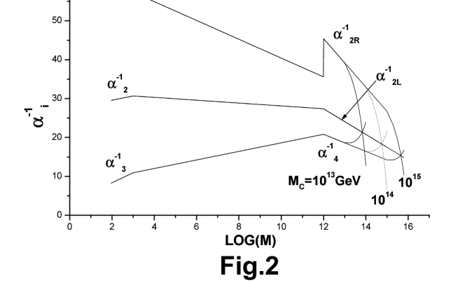
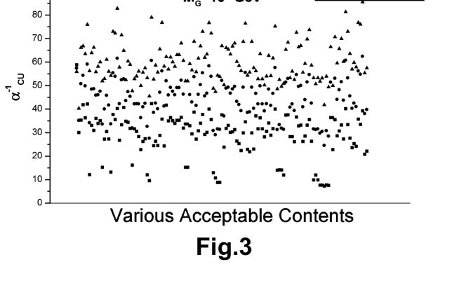
In Fig. 2 we show the running of the coupling constants for the above content and for several values of $M_{C}$. In Fig. 3 a scatter plot is presented showing the (inverse) of the unified coupling for several contents of the model.

Figure 2: The inverse of the three gauge couplings as a function of energy, for the $SU(4)\times SU(2)_{L}\times SU(2)_{R}$ GUT with the specific content appearing in (12). We have chosen $M_{G}=10^{12}$GeV and three values of the compactification scale $M_{C}=10^{13},10^{14},10^{15}$GeV.

Figure 3: Scatter plot of the inverse of the unified gauge coupling, for the $SU(4)\times SU(2)_{L}\times SU(2)_{R}$ GUT, choosing $M_{G}=10^{12}$GeV for three values of the compactification scale $M_{C}=10^{13},10^{14},10^{15}$GeV. The horizontal axes enumerates the various acceptable contents of the model (the order of appearance along the $x$–axis is irrelevant). The highest the compactification scale the greater the value of the $\alpha_{CU}$.

The $SU(3)_{C}\times U(3)_{L}\times U(3)_{R}$ model

Another interesting string derived model, which admits a low (intermediate) unification scale (no dangerous dimension–six operators), is based on the $SU(3)\times SU(3)_{L}\times SU(3)_{R}$ symmetry. The MSSM content is found in the $27$ representation of the $E_{6}$ group

$$27\rightarrow(3,{\bar{3}},1)+({\bar{3}},1,3)+(1,3,{\bar{3}}).$$ (13)

where

$$(3,{\bar{3}},1)=\left(\begin{array}[]{c}u\\ d\\ D\end{array}\right),({\bar{3}},1,3)=\left(\begin{array}[]{c}u^{c}\\ d^{c}\\ D^{c}\end{array}\right),(1,3,{\bar{3}})=\left(\begin{array}[]{ccc}h^{0}&h^{+}&e^{c}\\ h^{-}&{\bar{h}}^{0}&\nu^{c}\\ e&\nu&N\end{array}\right).$$ (14)

The breaking chain we adopt here is the following: the first group is the colour $SU(3)$. The second breaks to $SU(2)_{L}\times U(1)_{L}$, while the third breaks to a $U(1)_{R}$. The SM $U(1)_{Y}$ emerges as a linear combination of the two $U(1)_{L,R}$. The conventional hypercharge $Y$ is related to the $X$ and $Z$ charges of $U(1)_{L}$ and $U(1)_{R}$ correspondingly, by the relation

$$Y=\frac{1}{\sqrt{5}}X+\frac{2}{\sqrt{5}}Z,$$

while the corresponding relations of the couplings at the breaking scale is

$$\alpha_{L}=\alpha_{2},\quad\alpha^{-1}_{R}=(5/4)\alpha^{-1}_{Y}-(1/4)\alpha^{-1}_{L}.$$

Apart from the above states, in the string model, fractionally charged and other exotic states usually appear, belonging to the representations

$$\begin{array}[]{|c|c|c|}\hline\cr(\stackrel{{\scriptstyle(-)}}{{3}},1,1)&(1,\stackrel{{\scriptstyle(-)}}{{3}},1)&(1,1,\stackrel{{\scriptstyle(-)}}{{3}})\\ \hline\cr 0&\pm 1/3{\mbox{ and}}\pm 2/3&\pm 1/3{\mbox{ and}}\pm 2/3\\ \hline\cr\end{array}$$ (15)

where the second line shows the corresponding (electric) charges. One should not be misled by the values of these charges: the neutral states are coloured, while the others are singlet under the colour group. Therefore, after the symmetry breaking, these states will result in exotic lepton doublets and singlets carrying charges like those of the down and up quarks. Note that such states are not common in GUTs, however, they are generic in string models.

The one–oop $\beta$–functions are given by

$$\beta_{3} = -9+\frac{1}{2}\left(3n_{Q}+3n_{Q^{c}}+n_{C}\right)$$ (16)

$$\beta_{L} = -9+\frac{1}{2}\left(3n_{Q}+3n_{L}+n_{L^{\prime}}\right)$$ (17)

$$\beta_{R} = -9+\frac{1}{2}\left(3n_{Q^{c}}+3n_{L}+n_{L^{\prime\prime}}\right),$$ (18)

where $n_{Q}$, $n_{Q^{c}}$ and $n_{L}$ are the number of the representations appearing in the complete 27, Eq. (13), while $n_{C}$, $n_{L^{\prime}}$ and $n_{L^{\prime\prime}}$ are the number of the exotic representations of (15).

As in the case of the previous model, several massless spectra pass the two conditions and provide unification of the three couplings. Although it seems that the $SU(3)^{3}$ is probably less constrained (giving a lot of possible contents, presumably because of the symmetric form of the $\beta$-functions), one should be careful, since the unification coupling could be high enough in some cases and get out of the perturbative region. This of course happens for high matter content, when the $\beta$–functions become large and positive. We should note at this point (and it is a general remark not applicable only to the specific GUT) that the value of $M_{C}$ starts playing a significant role in the case where the unification coupling constant is getting large: if the $\beta$-functions between $M_{G}$ and $M_{C}$ are already large, $M_{C}$ cannot be much larger than $M_{G}$ if we want to avoid a non-perturbative value of the unification coupling.

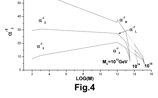
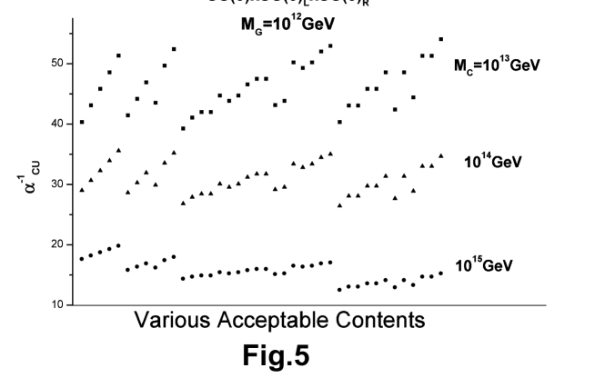
In the following table, we give, as an example, the content below and above $M_{C}$, for the $SU(3)^{3}$ model, where we have chosen $M_{G}=10^{12}$ GeV and a 3% error in the equality of the ratios

$$\begin{array}[]{lcccccc}&n_{Q}&n_{L}&n_{Q^{c}}&n_{C}&n_{L^{\prime}}&n_{L^{\prime\prime}}\\ {\mbox{ below }M_{C}}&10&4&6&10&0&2\\ {\mbox{ above }M_{C}}&6&0&2&10&0&2\,.\end{array}$$ (19)

In Fig. 4 we show the running of the couplings for the above content and for several values of $M_{C}$ while Fig. 5 is a scatter plot of the (inverse of the) inified coupling foe several contents of the model.

Figure 4: Same as in Fig.2 for the $SU(3)\times SU(3)_{L}\times SU(3)_{R}$ model and the specific content of (19).

Figure 5: Same as in Fig.3 for the $SU(3)\times SU(3)_{L}\times SU(3)_{R}$ model.

We conclude with a few remarks: the possibility of lowering the unification scale is a fascinating one, both from the theoretical and from the experimental point of view. Experimentally, it would be exciting to have a low enough unification scale for the possibility of testing its implications in the near–future machines. Theoretically, it would give a solution to the desert-puzzle invoked in previous Planck–mass unification scenarios. However, when lowering the unification scale in most of the GUTs, one faces the notorious problem of proton decay. A possible solution, which combines the idea of a relatively low unification and a reasonable solution to the proton decay problem, is the one presented in this note. We have considered GUTs that do not lead to proton decay via dimension-six operators and implemented the idea that the unification occurs at an intermediate scale so that, for appropriate Yukawa couplings, other dangerous operators may be sufficiently suppressed. We have shown that there exist numerous cases of massless spectra (which can be derived from the superstring), implying naturally intermediate scale unification.

References

[1]I. Antoniadis and B. Pioline, Nucl. Phys.
B 550 (1999) 41, [hep-th/9902055].
[2]
I. Antoniadis, Phys. Lett. B 246 (1990) 377.
[3]
K. Dienes, E. Dudas and T. Gherghetta, Phys. Lett. B 436
(1998) 55; hep-ph/9806292.
[4]
D. Ghilencea and G.G. Ross, Phys. Lett. B 442 (1998) 165.
[5]
K. Benakli, hep-ph/9809582.
[6]
C.P. Burges, L.E. Ibañez and F. Quevedo,
hep-ph/9810535;
L.E. Ibañez, C. Muñoz and S. Rigolin,
hep-ph/9812397;
T. Li,
hep-ph/9903371.
[7]A. Delgado and M. Quiros, hep-ph/9903400.
[8]G.K. Leontaris and N.D. Tracas, hep-ph/9902368.
[9]N.D. Tracas, talk given at the “XIth Rencontres de Blois
Frontiers of Matter, June 1999, to appear in the proceedings.
[10]I. Antoniadis, G.K. Leontaris and N.D. Tracas,
Phys. Lett. B 279 (1992) 58.