Soft Thermal Loops in Scalar Quantum Electrodynamics

Abstract

Scalar QED is used to study approximations in thermal field theory beyond the Hard Thermal Loop resummation scheme. For this purpose the photon self energy is calculated for external momenta of the order $e^{2}T$ using Hard Thermal Loop resummed Green functions.

Keywords: thermal field theory, Hard Thermal Loop resummation

During the last years thermal field theory became increasingly important for investigating problems in nuclear physics and astrophysics. Famous examples are the prediction of signatures for the quark-gluon plasma formation in relativistic heavy ion collisions [1], the origin of the baryon asymmtery in the early universe [2], and neutrino induced reactions in supernovae [3].

Perturbative calculations based on bare propagators and vertices, however, turned out to be inconsistent, i.e., they lead to gauge dependent and infrared divergent results. The reason for this failure is that at finite temperature (and density) higher order loop diagrams can contribute to lower order in the coupling constant. This problem has been solved within the Hard Thermal Loop (HTL) resummation technique invented by Braaten and Pisarski [4]. The basic idea is that one has to distinguish between momentum scales $T$, called hard, and $gT$, called soft, in the weak coupling limit $g\ll 1$. Now, the leading order contribution to self energies and vertices with soft external momenta comes from one loop diagrams containing only hard momenta. By resumming these HTLs, effective propagators and vertices are constructed containing medium effects such as Debye screening. These effective Green functions have to be used if their momenta are soft, while bare Green functions are sufficient for hard momenta. In this way, quantities, in which only scales of the order $T$ and $gT$ are involved, can be treated consistently.

However, problems being sensitive to the scale $g^{2}T$, such as damping rates of hard quarks and gluons in the quark-gluon plasma [5] and the sphaleron rate possibly related to baryogenesis in the early universe [6], cannot be treated in this way. The super soft scale $g^{2}T$ arises from the transverse part of the massless gauge boson propagator, which shows in the HTL approximation no screening in the static limit, i.e. no screening of static magnetic fields. Therefore quantities involving the transverse gauge boson propagator at scales $g^{2}T$ or smaller exhibit infrared singularities, although HTL resummed propagators are used. For example, the damping rate of hard partons calculated within the HTL resummation method suffers from a logarithmic infrared divergence [5].

For dealing with the momentum scale $g^{2}T$, one has to go beyond the HTL approximation. For static quantities, such as the thermodynamic quantities entropy, free energy, energy density, and pressure, an approximation beyond the HTL method based on an effective high temperature field theory has been derived using dimensional reduction [7]. For dynamical quantities, e.g. particle production and interaction rates, the super soft scale has been considered in the non-abelian case using a Langevin equation for the gauge fields [8]. This Langevin equation is related to the self energies of the gauge boson at super soft external momentum [9]. In order to calculate this self energy one has to consider diagrams containing soft momenta, which we will call Soft Thermal Loops (STL) in the following. The explicit evaluation of these diagrams is very involved, because one has to use HTL propagators and vertices. As an example we show the STL photon self energy in Fig.1, where blobs denote HTL Green functions.

In the case of scalar QED, however, STLs can be computed easily and analytic expressions can even be given as we will see in the following. Calculations are facilitated for scalar QED significantly by the fact that HTL effective vertices are absent and the HTL scalar self energy is momentum independent [10]. After all scalar QED is a gauge theory which shows a sensitivity to the scale $g^{2}T$ in the gauge boson sector, i.e., it suffers from the absence of static magnetic screening in the same way as QED and non-abelian gauge theories. Therefore scalar QED has been used as a toy model in a number of papers for studying problems in finite temperature gauge field theories [10, 11]. A possible application of scalar QED at finite temperature might be the formation of topological defects in the early universe [12]. Also it can be easily extended to the Higgs sector of the electroweak theory in the symmetric phase [13].

The aim of the present investigation is the computation of the STL photon self energy in scalar QED, which is the basic ingredient for going beyond the HTL resummation scheme.

Since there are no HTL vertices in scalar QED, the STL photon self energy is given by the diagrams shown in Fig.2. Using the real time formalism within the Keldysh representation (see e.g. [14]), the retarded, advanced, and symmetric scalar HTL propagator, assuming a vanishing bare scalar mass, is given by

$$\Delta_{R,A}^{*}(K) = \frac{1}{K^{2}-m_{s}^{2}\pm isgn(k_{0})\epsilon}\,,$$ (1)

$$\Delta_{F}^{*}(K) = -2\pi i\>[1+2n_{B}(|k_{0}|)]\>\delta(K^{2}-m_{s}^{2})\,,$$ (2)

where we have used the notation $K=(k_{0},{\bf k})$, $k=|{\bf k}|$, and $n_{B}(x)=1/[\exp(x/T)-1]$ denotes the Bose distribution function. The effective, temperature dependent scalar mass is given by $m_{s}=eT/2$ [10]. Although the one-loop scalar self energy contains a polarization diagram with two internal photon lines, it reduces to a momentum independent mass term in the HTL approximation. Similar there are no effective HTL vertices in the HTL approximation, which can be traced back to the absence of $\gamma$-matrices in the bare vertices. Therefore the STL photon self energy differs from the HTL self energy only by the presence of the effective scalar mass $m_{s}$.

Let us first discuss the tadpole contribution of Fig.2. Using the real time formalism the retarded self energy contribution can be written as

$${}^{tad}{\Pi_{R}^{*}}^{\mu\nu}=-ie^{2}\>g^{\mu\nu}\>\int\frac{d^{4}K}{(2\pi)^{4}}\>[\Delta_{F}^{*}(K)+\Delta_{R}^{*}(K)+\Delta_{A}^{*}(K)]\,.$$ (3)

Now, assuming the external legs of this self energy to be super soft, we want to extract the leading order correction to the HTL self energy. This correction is of order $e^{3}$ and comes entirely from the part containing the distribution function in (3) [15]. The terms without distribution functions lead to a correction of order $e^{4}$ and will be neglected [5]. After integrating over $k_{0}$ by means of the $\delta$-functions in (2) and trivially over the angles, (3) reduces to

$${}^{tad}{\Pi_{R}^{*}}^{\mu\nu}\simeq-\frac{e^{2}}{\pi^{2}}\>g^{\mu\nu}\>\int_{0}^{\infty}dk\>\frac{k^{2}}{\omega_{k}}\>n_{B}(\omega_{k})\,,$$ (4)

where $\omega_{k}^{2}=k^{2}+m_{s}^{2}$. The order $e^{3}$ contribution can be extracted by introducing a separation scale $eT\ll\Lambda\ll T$. Decomposing the integral in (4) in two parts, where we integrate in the first one from zero to $\Lambda$ and in the second one from $\Lambda$ to infinity, we may expand the distribution function in the first integral for small arguments and neglect $m_{s}$ of order $eT$ in the second. Then we end up with

$${}^{tad}{\Pi_{R}^{*}}^{\mu\nu}=-\frac{3}{2}\>g^{\mu\nu}\>m_{\gamma}^{2}\>\left(1-\frac{3}{2\pi}e\right)+O(e^{4})\,,$$ (5)

where $m_{\gamma}=eT/3$ is identical to the plasma frequency in the HTL limit. The HTL result is given by the first term proportional to $e^{2}$ in (5).

For calculating the polarization diagram of Fig.2 it is convenient to decompose it into a longitudinal and transverse part. Using the real time formalism the second diagram of Fig.2 leads to

$${}^{pol}{\Pi_{R}^{*}}^{L}=i\frac{e^{2}}{2}\>\int\frac{d^{4}K}{(2\pi)^{4}}\>(q_{0}+k_{0})^{2}\>[\Delta_{F}^{*}(Q)\Delta_{R}^{*}(K)+\Delta_{A}^{*}(Q)\Delta_{F}^{*}(K)]\,,$$ (6)

where $Q=K-P$. Since the internal scalar propagators are never super soft due to the presence of the effective scalar mass of the order $eT$, the integrands in (6) can be expanded for super soft $p,p_{0}\ll\omega_{k}$. This expansion is analogous to the one for extracting the HTL contribution, where the internal momenta are assumed to be hard, while the external are soft. Then (6) yields

$${}^{pol}{\Pi_{R}^{*}}^{L}\simeq\frac{e^{2}}{\pi^{2}}\>\>\int_{0}^{\infty}dk\>k\>n_{B}(\omega_{k})\>\left(\frac{p_{0}}{p}\,\ln\frac{p_{0}\omega_{k}+pk+i\epsilon}{p_{0}\omega_{k}-pk+i\epsilon}-P^{2}\,\frac{\omega_{k}k}{p_{0}^{2}\omega_{k}^{2}-p^{2}k^{2}}\right).$$ (7)

For $\omega_{k}=k$ this expression reduces to the HTL result

$${}^{pol}\Pi_{R}^{L}=-\frac{e^{2}T^{2}}{6}\left(1-\frac{p_{0}}{p}\,\ln\frac{p_{0}+p+i\epsilon}{p_{0}-p+i\epsilon}\right).$$ (8)

Proceeding similar as for the tadpole by introducing a separation scale $\Lambda$, the leading order correction follows from

$${}^{pol}{\Pi_{R}^{*}}^{L} \simeq\frac{e^{2}T^{2}}{\pi^{2}}\>\Biggl{\{}\frac{\pi^{2}}{6}\left(\frac{p_{0}}{p}\,\ln\frac{p_{0}+p}{p_{0}-p}-1\right)$$ (10)

$$-\frac{1}{T}\int_{0}^{\infty}dk\left[\frac{p_{0}}{p}\,\ln\frac{p_{0}+p}{p_{0}-p}-1-z\left(\frac{p_{0}}{p}\,\ln\frac{p_{0}+pz}{p_{0}-pz}-P^{2}\,\frac{z}{p_{0}^{2}-p^{2}z^{2}}\right)\right]\Biggr{\}}\,,$$

where $z=k/\omega_{k}$ and we neglected $i\epsilon$. Using the substitution $k\rightarrow z$ the integral in (10) can be evaluated analytically resulting in

$${\Pi_{R}^{*}}^{L}=\Pi_{R}^{L}+\frac{e^{3}T^{2}}{4\pi}\left(1-\frac{p_{0}}{\sqrt{p_{0}^{2}-p^{2}}}\right)+O(e^{4})\,,$$ (11)

where the tadpole contribution (5) has been added and

$$\Pi_{R}^{L}=-3\,m_{\gamma}^{2}\>\left(1-\frac{p_{0}}{2p}\,\ln\frac{p_{0}+p}{p_{0}-p}\right)$$ (12)

is the longitudinal HTL self energy [16].

Analogously one finds for the transverse part of the photon self energy

$${\Pi_{R}^{*}}^{T}=\Pi_{R}^{T}+\frac{e^{3}T^{2}}{4\pi}\left[\left(1-\frac{p_{0}^{2}}{p^{2}}\right)\>\left(1-\frac{p_{0}}{\sqrt{p_{0}^{2}-p^{2}}}\right)-1\right]+O(e^{4})\,,$$ (13)

where the transverse HTL self energy is given by [16]

$$\Pi_{R}^{T}=\frac{3}{2}\,m_{\gamma}^{2}\,\frac{p_{0}^{2}}{p^{2}}\>\left[1-\left(1-\frac{p^{2}}{p_{0}^{2}}\right)\,\frac{p_{0}}{2p}\,\ln\frac{p_{0}+p}{p_{0}-p}\right]\,.$$ (14)

Actually the STL transverse photon self energy is more interesting because transverse photons are sensitive to the scale $e^{2}T$ due to the missing static magnetic screening. The photon self energy (11) and (13) agrees with the expressions given in Ref.[10] in the super soft momentum limit $p_{0},p\sim e^{2}T$.

Now we want to discuss our results. First we observe that in contrast to non-abelian theories there is no STL correction to order $e^{2}$ for super soft external momenta as already noted by Bödeker [9]. Secondly, we note that our result (11) and (12) are gauge invariant, since $m_{s}$ is a gauge invariant quantity. Next, we see that the self energies given here possess an imaginary part only below light cone $p_{0}^{2}<p^{2}$ as the HTL self energies do. However, the imaginary part comes now from a square root instead of a logarithm.

Finally, we want to study the zero momentum limits of our self energies. In the limit $p\rightarrow 0$ the expressions in (11) and (13) reduce to

$${\Pi_{R}^{*}}^{L}(p=0) = \frac{p^{2}}{p_{0}^{2}}\,\left(m_{\gamma}^{2}-\frac{e^{3}T^{2}}{8\pi}\right)\,,$$ (15)

$${\Pi_{R}^{*}}^{T}(p=0) = m_{\gamma}^{2}-\frac{e^{3}T^{2}}{8\pi}\,.$$ (16)

Hence the dielectric functions defined by $\epsilon_{L}=1-\Pi_{L}/p^{2}$ and $\epsilon_{T}=1-\Pi_{T}/p_{0}^{2}$ [17] agree in this limit as expected, since there is no direction preferred for $p=0$ [18]. The result (16) should not be confused with the plasma frequency, which is given by ${\Pi_{R}^{*}}^{L,T}(p_{0}=m_{\gamma},p=0)$ [10]. This limit has not been studied here as we assumed that $p_{0}\sim e^{2}T$. Also we cannot consider the plasmon dispersion relation from our self energies (11) and (13), since $p_{0}\geq m_{\gamma}$ for real plasma modes. In the limit $p_{0}\rightarrow 0$, on the other hand, the self energies read

$${\Pi_{R}^{*}}^{L}(p_{0}=0) = -3m_{\gamma}^{2}\left(1-\frac{3e}{4\pi}\right)\,,$$ (17)

$${\Pi_{R}^{*}}^{T}(p_{0}=0) = \Pi_{R}^{T}(p_{0}=0)=0\,.$$ (18)

The result for the longitudinal component determines the correction to the Debye screening mass, which is given by $m_{D}^{2}=3m_{\gamma}$ in the HTL approximation and agrees with the one found in Ref.[10, 20]. As expected [20] there is no static magnetic screening mass in scalar QED even beyond the HTL approximation.

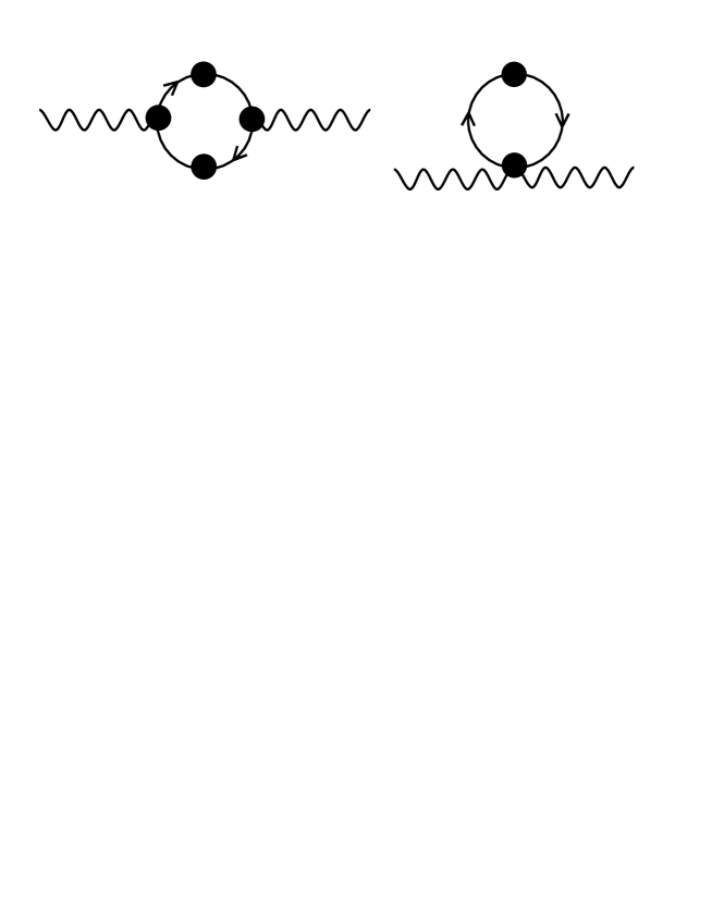
FIG. 1.: STL photon self energy in QED. The blobs denote HTL resummed electron propagators and photon-electron vertices.

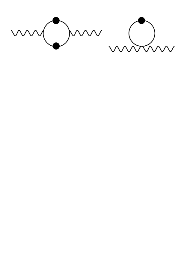
FIG. 2.: STL photon self energy in scalar QED. The blobs denote HTL resummed scalar propagators.

REFERENCES

- [1] B. Müller, Nucl. Phys. A630 (1998) 461c.
- [2] A.G. Cohen, D.B. Kaplan, and A.E. Nelson, Ann. Rev. Nucl. Part. Sci. 43 (1993) 27.
- [3] G.G. Raffelt, Stars as Laboratories for Fundamental Physics: The Astrophysics of Neutrinos, Axions, and other Weakly Interacting Particles (University Press, Chicago, 1996).
- [4] E. Braaten and R.D. Pisarski, Nucl. Phys. B 337 (1990) 569.
- [5] For a review see: M.H. Thoma, in Quark Gluon Plasma 2, ed. R.C. Hwa (World Scientific, Singapore, 1995) p.51.
- [6] P. Arnold and L. McLerran, Phys. Rev. D 36 (1987) 581.
- [7] K. Kajantie, M. Laine, K. Rummukainen, and M.Shaposhnikov, Nucl. Phys. B 458 (1996) 90.
- [8] D. Bödeker, Phys. Lett. B 426 (1998) 351 and hep-ph/9905239.
- [9] D. Bödeker, hep-ph/9903478.
- [10] U. Kraemmer, A.K. Rebhan, and H. Schulz, Ann. Phys. (N.Y.) 238 (1995) 286.
- [11] M.H. Thoma and C.T. Traxler, Phys. Lett. B 378 (1996) 233; D. Boyanovsky, H.J. de Vega, R. Holman, S.P. Kumar, and R.D. Pisarski, Phys. Rev. D 58 (1998) 125009.
- [12] T. Vachaspati, hep-ph/9710292.
- [13] T.S. Biró and M.H. Thoma, Phys. Rev. D 54 (1996) 3465.
- [14] M.E. Carrington, H. Defu and M.H. Thoma, Eur. Phys. J. C 7 (1999) 347.
- [15] J.I. Kapusta, Finite Temperature Field Theory (Cambridge University press, New York, 1989).
- [16] V.V. Klimov, Sov. Phys. JETP 55 (1982) 199; H.A. Weldon, Phys. Rev. D 26 (1982) 1394.
- [17] H.T. Elze and U. Heinz, Phys. Rep. 183 (1989) 81.
- [18] E.M. Lifshitz and L.P. Pitajewski, Physical Kinetics (Pergamon, New York, 1981).
- [19] A.K. Rebhan, Phys. Rev. D 48 (1993) R3967.
- [20] J.P. Blaizot, E, Jancu, and R.R. Parwani, Phys. Rev. D 52 (1995) 2543.