Power corrections and resummation of radiative corrections in the single dressed gluon approximation – the average thrust as a case study

Abstract:

Infrared power corrections for Minkowskian QCD observables are analyzed in the framework of renormalon resummation, motivated by analogy with the skeleton expansion in QED and the BLM approach. Performing the “massive gluon” renormalon integral a renormalization scheme invariant result is obtained. Various regularizations of the integral are studied. In particular, we compare the infrared cutoff regularization with the standard principal value Borel sum and show that they yield equivalent results once power terms are included. As an example the average thrust $\left<T\right>$ in $e^{+}e^{-}$ annihilation is analyzed. We find that a major part of the discrepancy between the known next-to-leading order calculation and experiment can be explained by resummation of higher order perturbative terms. This fact does not preclude the infrared finite coupling interpretation with a substantial $1/Q$ power term. Fitting the regularized perturbative sum plus a $1/Q$ term to experimental data yields $\alpha_{s}^{\hbox{$\overline{\hbox{\tiny MS}}\,$}}({\rm M_{Z}})=0.110\pm 0.002$.

1 Introduction

Power corrections in QCD have been the subject of many interesting theoretical developments in the recent years [1], especially concerning observables that do not admit an operator product expansion. Of particular interest in this respect are event shape variables in $e^{+}e^{-}$ annihilation. For these observables the available [2] next-to-leading order perturbative calculations in a standard choice of renormalization scheme and scale are found not to agree with experimental data [3]. The discrepancy was originally bridged over by Monte-Carlo simulations which account for non-perturbative “hadronization corrections”. The data can also be fitted by the next-to-leading order perturbative result plus a power correction that typically (but not always) falls as $1/Q$, where $Q=\sqrt{s}$ is the center of mass energy. Nevertheless, this situation is not satisfactory, especially because the non-perturbative correction, which is not under control theoretically, is numerically quite significant. Consequently, much theoretical effort has been invested in the last five years in understanding the source of these power corrections. This effort turned out to be quite fruitful [4]–[11]: a “renormalon phenomenology” has been developed [1], where information contained in perturbation theory is used to determine the form of the power correction, while its normalization is left as a non-perturbative parameter, which is determined by fitting experimental data.

On the other hand, the very same observables appear to have significant sub-leading perturbative corrections and large renormalization scheme and scale dependence when calculated up to the next-to-leading order, as discussed in ref. [12, 13, 3]. This observation raises concern about the reliability of the results obtained in the usual procedure, where a perturbative expansion truncated at the next-to-leading order is used as a starting point for the experimental fit [3]. Unfortunately, the full next-to-next-to-leading order calculation for these observables is not yet available.

In this paper, we adopt the view that the most important corrections are related to the running of the coupling, in the spirit of the BLM approach [15]. Following [16], we assume that the perturbative series can be reshuffled in a (yet hypothetical) “dressed skeleton expansion” built in analogy with the Abelian theory, where each term is by itself renormalization scheme invariant. This expansion was the original motivation behind the BLM approach (see ref. [17] for further discussion). In the Abelian theory, the skeleton expansion is well defined. The first term corresponds to an exchange of a single photon, dressed by all possible vacuum polarization insertions which build up the Gell-Mann Low effective-charge; the second term corresponds to an exchange of two dressed photons and so on. The expansion coincides with the standard expansion in $\alpha$ for a conformal theory where the coupling does not run. The leading skeleton term can be written compactly as a “renormalon integral” – an integral over all scales of the Gell-Mann Low effective-charge times an observable dependent function which arises from the one-loop Feynman integrand and represents the momentum distribution of the exchanged dressed photon. When the leading skeleton term is expanded in terms of the coupling up to large enough order, both large and small momentum regions give rise to factorially increasing perturbative coefficients. These are the renormalons [18]–[21] which are believed to dominate the diverging large order behavior of the full perturbative series. This way renormalons carry information about the inconsistency of perturbation theory and thus on possible non-perturbative power corrections arising from the strong coupling regime.

Having no straightforward diagrammatic interpretation in the non-Abelian case the “skeleton expansion” is still just a conjecture. There is an obvious difficulty due to gluon self-interaction vertices. This difficulty can be hopefully resolved by separating contributions from such diagrams into several different skeleton terms in a gauge invariant manner. Ref. [22] gives a concrete suggestion for a diagrammatic construction of the skeleton expansion in QCD, based on the pinch technique. However, more work is required to establish it beyond the one-loop level. On the other hand, the structure of the single gluon exchange term (“leading skeleton”) is strongly motivated by the large $N_{f}$ limit where the Abelian correspondence is transparent. The non-Abelian analogue of the renormalon integral, obtained through the “Naive Non-Abelianization” [23] procedure, was used extensively in the last few years in all order perturbative resummation (e.g. [24]–[27]) and parametrization of power corrections (e.g. [6]–[11] and [16]).

In the present work, we perform an analysis of infrared power corrections together with all order perturbative resummation of renormalon-type diagrams in the “massive gluon” approach [24, 25, 8]. We show that these two aspects of improving the standard perturbative calculation cannot be dissociated and must be performed together.

We study one specific example: the average thrust in $e^{+}e^{-}$ annihilation, where there is a priori evidence for both large perturbative corrections and strong $1/Q$ power corrections. We perform renormalon resummation at the level of a single gluon emission, emphasizing the renormalization group invariance of this procedure. We discuss in detail the ambiguity between the perturbative sum and the non-perturbative infrared power corrections. We also address the complications that arise when applying the inclusive “massive gluon” resummation to not-completely-inclusive Minkowskian observables, such as the example at hand.

The paper is organized as follows: in sec. 2 we describe the specific assumptions we make concerning the “dressed skeleton expansion” in QCD and the immediate consequences that follow. We also compare the “skeleton expansion” with the BLM scale fixing procedure. In sec. 3 we discuss various natural regularizations of the perturbative sum, concentrating on Minkowskian quantities. In sec. 4 we show that the regularization independence of the full QCD result is achieved only by adding to the regularized perturbative sum explicit power terms. We also discuss the connection with the infrared finite coupling approach [7, 8]. In sec. 5 we present the application of the method to the average thrust. Sec. 6 contains our conclusions.

2 The “dressed skeleton expansion” and BLM

Consider first a generic Euclidean quantity $D(Q^{2})$, which has the perturbative expansion

$$D_{\hbox{\tiny PT}}(Q^{2})=r_{0}a+r_{1}a^{2}+\cdots$$ (1)

where $a\equiv{\alpha_{s}\over\pi}$ is the coupling at scale $\mu_{R}^{2}$ in (say) the ${\rm\overline{MS}}$ scheme. Since the leading coefficient $r_{0}$ is flavor independent and the next-to-leading coefficient $r_{1}$ is linear in $N_{f}$, one can write

$$r_{1}=r_{0}\left[-\beta_{0}\left(\log{Q^{2}\over\mu_{R}^{2}}+\gamma_{1}\right)+\delta_{1}\right]$$ (2)

where

$$\beta_{0}={1\over 4}\left({11\over 3}N_{c}-{2\over 3}N_{f}\right)$$ (3)

is the one-loop $\beta$ function coefficient, $\,\beta(a)\,=\,da/d\ln\mu_{R}^{2}=-\beta_{0}a^{2}+\cdots\,$, and $\gamma_{1}$ and $\delta_{1}$ are flavor independent. We shall assume, in analogy with QED, that $D_{\hbox{\tiny PT}}(Q^{2})$ has the “dressed skeleton expansion”

$$D_{\hbox{\tiny PT}}(Q^{2})=D_{0}^{\hbox{\tiny PT}}(Q^{2})+D_{1}^{\hbox{\tiny PT}}(Q^{2})+\cdots$$ (4)

where $D_{0}^{\hbox{\tiny PT}}$ is the contribution of a single dressed gluon exchange, $D_{1}^{\hbox{\tiny PT}}$ comes from a double exchange, etc. This means in particular that we assume for $D_{0}^{\hbox{\tiny PT}}$ the representation

$$D_{0}^{\hbox{\tiny PT}}(Q^{2})\equiv\int_{0}^{\infty}{dk^{2}\over k^{2}}\ \bar{a}_{\hbox{\tiny PT}}(k^{2})\,\Phi_{D}(k^{2}/Q^{2})$$ (5)

where $\Phi_{D}$ is the “momentum distribution function” [26] which depends on the observable under consideration ($D$), whereas $D_{1}^{\hbox{\tiny PT}}$ would be given by

$$D_{1}^{\hbox{\tiny PT}}(Q^{2})\equiv\int_{0}^{\infty}{dk_{1}^{2}\over k_{1}^{2}}\,{dk_{2}^{2}\over k_{2}^{2}}\,\bar{a}_{\hbox{\tiny PT}}(k_{1}^{2})\,\bar{a}_{\hbox{\tiny PT}}(k_{2}^{2})\,\Phi_{D}^{1}(k_{1}^{2}/Q^{2},k_{2}^{2}/Q^{2})$$ (6)

and so on. The physical “skeleton coupling” $\bar{a}_{\hbox{\tiny PT}}$ appearing in both (5) and (6) does not depend on the observable under consideration. It is supposed to be uniquely determined and is a priori different from the renormalization scheme coupling $a\equiv a(\mu_{R}^{2})$. We can therefore consider its (a priori non-trivial) expansion in the renormalization scheme coupling

$$\bar{a}_{\hbox{\tiny PT}}(k^{2})=a\,+\,\left[-\beta_{0}\left(\log{k^{2}\over\mu_{R}^{2}}+c_{1}\right)+d_{1}\right]\,a^{2}\,+\,\cdots$$ (7)

Using eq. (7) in eq. (5) we obtain

$$D_{0}^{\hbox{\tiny PT}}(Q^{2})=r_{0}a+r_{1}^{0}a^{2}+\cdots$$ (8)

with $r_{0}=\phi_{0}$ and

$$r_{1}^{0}=\phi_{0}\left[-\beta_{0}\left(\log{Q^{2}\over\mu_{R}^{2}}+{\phi_{1}\over\phi_{0}}+c_{1}\right)+d_{1}\right]$$ (9)

where $\phi_{i}$ are the log-moments of the momentum distribution function,

$$\phi_{i}\equiv\int_{0}^{\infty}{dk^{2}\over k^{2}}\ \left(\log{k^{2}\over Q^{2}}\right)^{i}\ \Phi_{D}(k^{2}/Q^{2}).$$ (10)

The only source of $N_{f}$ dependence in the next-to-leading order coefficient $r_{1}$ are vacuum polarization corrections which dress the exchanged gluon, namely corrections that are fully included in $D_{0}^{\hbox{\tiny PT}}(Q^{2})$. It therefore follows that the “Abelian” parts proportional to $\beta_{0}$ in $r_{1}$ and $r_{1}^{0}$ are the same, i.e.

$$r_{0}\gamma_{1}=\phi_{1}+\phi_{0}c_{1}.$$ (11)

The next observation is that the “leading skeleton” term $D_{0}^{\hbox{\tiny PT}}(Q^{2})$ is a renormalization scheme invariant quantity, just as the “skeleton coupling” $\bar{a}_{\hbox{\tiny PT}}(k^{2})$ itself. The question whether the approximation of $D_{\hbox{\tiny PT}}(Q^{2})$ by $D_{0}^{\hbox{\tiny PT}}(Q^{2})$ is a good one thus has a renormalization scheme invariant meaning. In particular the leading order correction, which is ${\cal O}(a^{2})$, can be written as

$$D_{\hbox{\tiny PT}}(Q^{2})\simeq D_{0}^{\hbox{\tiny PT}}(Q^{2})+(r_{1}-r_{1}^{0})\,a^{2}+\cdots$$ (12)

where $r_{1}-r_{1}^{0}$ is renormalization scheme invariant. Note that

$$r_{1}-r_{1}^{0}=r_{0}\left(\delta_{1}-d_{1}\right)$$ (13)

and the r.h.s. can be identified as the difference between the next-to-leading coefficients which remain after performing BLM scale setting [15] in the two renormalization group invariant quantities $D_{\hbox{\tiny PT}}(Q^{2})$ and $D_{0}^{\hbox{\tiny PT}}(Q^{2})$ respectively. Such a difference is known [15, 28] to be renormalization scheme invariant, although $\delta_{1}$ and $d_{1}$ are separately scheme dependent.

It is interesting to compare the “skeleton expansion” approach which we take here with the standard BLM scale setting procedure [15]:

1. Eq. (11) is equivalent to the statement that the BLM scale for the quantities $D_{\hbox{\tiny PT}}(Q^{2})$ and $D_{0}^{\hbox{\tiny PT}}(Q^{2})$ is the same:

$$\mu^{2}_{\hbox{\tiny BLM}}=Q^{2}\exp\left(\frac{\phi_{1}}{\phi_{0}}+c_{1}\right)=Q^{2}\exp(\gamma_{1})$$ (14)

with $\phi_{i}$ defined in (10). Note in particular that if BLM is applied in the “skeleton scheme”, where $a=\bar{a}_{\hbox{\tiny PT}}$, $c_{1}=0$ and then the BLM scale is the center [26, 29] of the momentum distribution $\Phi_{D}(k^{2}/Q^{2})$,

$$\mu^{2}_{\hbox{\tiny BLM}}=Q^{2}\exp\left(\frac{\phi_{1}}{\phi_{0}}\right)$$ (15)

i.e. it is the average virtuality of the exchanged dressed gluon. Using the BLM scale, the leading order term $r_{0}\,a(\mu_{\hbox{\tiny BLM}}^{2})$ can be viewed [26, 29] as an approximation to the entire all-order sum $D_{0}^{\hbox{\tiny PT}}(Q^{2})$. This approximation is good if $\Phi_{D}(k^{2}/Q^{2})$ is narrow, and it is exact for

$$\Phi_{D}(k^{2}/Q^{2})=r_{0}\,\delta\left(\frac{k^{2}}{Q^{2}}-\frac{\mu_{\hbox{\tiny BLM}}^{2}}{Q^{2}}\right).$$ (16)

2. The usual justification of BLM (in a generic scheme) relies on the assumption that $\delta_{1}$ is small and so the large $\beta_{0}$ piece $-\beta_{0}\left(\log{Q^{2}\over\mu_{R}^{2}}+\gamma_{1}\right)$ dominates the full next-to-leading coefficient $r_{1}$ in eq. (2). This depends on the renormalization scheme, scale and $N_{f}$. On the other hand, in the “skeleton expansion” approach there is no scale setting to perform, and so the accuracy of approximating $D_{\hbox{\tiny PT}}(Q^{2})$ by $D_{0}^{\hbox{\tiny PT}}(Q^{2})$ is controlled by the magnitude of a scheme invariant coefficient (13); the issue now is whether $d_{1}$ is a good approximation to $\delta_{1}$. Note also that if the quantities in eq. (13) are computed in the “skeleton scheme” then $d_{1}=0$ and the scheme invariant parameter that controls the accuracy of the “skeleton expansion” can be identified as the standard BLM coefficient $r_{0}\,\delta_{1}$.

As mentioned in the introduction, it is not yet clear whether a “skeleton expansion” exists in QCD. Thus we do not know the identity of the “physical skeleton coupling” $\bar{a}_{\hbox{\tiny PT}}$. We do know, however, that in the Abelian limit the “skeleton coupling” should coincide with the V-scheme and so the Abelian coefficient $c_{1}$ is determined. For instance, in the $\overline{\hbox{MS}}\,$ scheme, $c_{1}=-{5\over 3}$. In order to perform the “leading skeleton” resummation in practice we need to specify also the non-Abelian coefficient $d_{1}$. We shall therefore consider in this paper three schemes which share the same $c_{1}$ mentioned above and differ by $d_{1}$ (all quoted values are in $\overline{\hbox{MS}}\,$):

a) The “gluon bremsstrahlung” coupling [30], where $d_{1}^{\hbox{\tiny brem}}=1-{\pi^{2}\over 4}$. This coupling was used in [7, 8] for parametrization of power corrections to event-shape variables.

b) The skeleton effective charge found in [22] using the pinch technique, where $d_{1}^{\hbox{\tiny pinch}}=1$.

c) The V-scheme coupling [15], defined by the static heavy quark potential, where $d_{1}^{\hbox{\tiny V}}=-2$.

One might worry that without a precise identification of the “skeleton coupling” we introduce back some kind of renormalization scheme dependence. We shall see that in practice (sec. 5), the inclusion of a next-to-leading order correction as in (12) effectively compensates to a large extent for the ambiguity in $d_{1}$.

3 Regularization

We begin with the observation that the integrals representing the terms $D_{i}^{\hbox{\tiny PT}}$ in the “skeleton expansion”, e.g. $D_{0}^{\hbox{\tiny PT}}$ of eq. (5), are ill-defined since they run over the Landau singularity. This is the way the infrared renormalon ambiguity of the perturbative sum appears in the framework of the “skeleton expansion”. It is possible to make these renormalon integrals mathematically well-defined by specifying a formal procedure to avoid the Landau singularity. However, this would not cure the physical problem of infrared renormalons: some additional information associated with large distances is required in order to obtain the full QCD result from the perturbative one.

Still, in order to use the “skeleton expansion” in practice one is bound to define $D_{i}^{\hbox{\tiny PT}}$ somehow. We shall concentrate in this paper on the single dressed gluon term $D_{0}^{\hbox{\tiny PT}}$ and refer to the regularized integral of eq. (5) as the “sum of perturbation theory”. We shall consider various possible regularization prescriptions: Principal Value (PV) Borel summation, Analytic Perturbation Theory (APT) approach (“gluon mass integral”), infrared cutoff method, and truncation of the perturbative series at the minimal term. Any two such prescriptions differ just by power terms. Thus, the “dressed skeleton” approach leads us implicitly to the subject of power corrections.

It is clear that physics does not depend upon the definition used. In practice, having no way to calculate the non-perturbative contribution we shall just parametrize it properly and fit the data by the “sum of perturbation theory” plus a power term. The prescription dependence of the two separate contributions cancels by construction. While in principle any regularization can be used, some may be more illuminating then others. As we shall see in sec. 3.3 and later in sec. 4 the infrared cutoff regularization is of special interest, allowing to separate at once short vs. long distance physics and perturbative vs. non-perturbative physics.

The purpose of this section is to derive the general relations between different regularization prescriptions which are useful in the analysis of Minkowskian observables. We begin by discussing the application of the “skeleton expansion” to Minkowskian observables concentrating on the “leading skeleton” term. We review the Analytic Perturbation Theory (APT) or “gluon mass” [24, 25, 8, 16] integral which seems to be the most convenient regularization for a practical calculation of the perturbative sum (sec. 3.1). We then (sec. 3.2) discuss the power corrections that distinguish between the APT integral and the principal value Borel sum [24, 25, 16]. In sec. 3.3 we explain how an Euclidean infrared cutoff can be introduced for Minkowskian observables and derive the relation between the cutoff regularized perturbative sum and the APT integral. In sec. 3.4 we generalize the explicit formulae of sec. 3.2 and 3.3 to the case of a two-loop “skeleton coupling”, and finally, in sec. 3.5 we comment of the comparison between different regularizations. Appendix A describes an alternative computation method for the cutoff regularization in terms of the APT integral.

3.1 Minkowskian quantities and the APT integral

We assume that a “skeleton expansion” such as (4) can be constructed also for Minkowskian observables. For a Minkowskian observable which is related by a dispersion relation to an Euclidean quantity, linearity of the dispersion relation implies that the expansion will take the form

$$R_{\hbox{\tiny PT}}(Q^{2})\,=\,R_{0}^{\hbox{\tiny PT}}(Q^{2})+R_{1}^{\hbox{\tiny PT}}(Q^{2})+\cdots$$ (17)

where $R_{0}^{\hbox{\tiny PT}}$ is the leading “dressed skeleton” which is related to $D_{0}^{\hbox{\tiny PT}}$ by a dispersion relation [16]. Similarly, $R_{1}^{\hbox{\tiny PT}}$ should be related by a dispersion relation to $D_{1}^{\hbox{\tiny PT}}$ of eq. (6), and so on. If there is no dispersion relation with an Euclidean quantity, the existence of a “skeleton expansion” is more doubtful. In particular, as we discuss in sec. 5, there is presumably no way to replace the entire perturbative series of not-completely-inclusive observables such as weighted cross sections by a “skeleton expansion”.

Let us concentrate now on the “single dressed gluon approximation” $R_{0}^{\hbox{\tiny PT}}$. It turns out that $R_{0}^{\hbox{\tiny PT}}$ cannot be expressed in the “Euclidean” representation of eq. (5) as an integral over the space-like coupling $\bar{a}_{\hbox{\tiny PT}}$. Instead, $R_{0}^{\hbox{\tiny PT}}$ has a “Minkowskian” representation in terms of the time-like discontinuity of the coupling [24, 25, 26, 8], $R_{0}^{\hbox{\tiny PT}}=R_{\hbox{\tiny APT}}$ with

$$R_{\hbox{\tiny APT}}(Q^{2}) \equiv \int_{0}^{\infty}{d\mu^{2}\over\mu^{2}}\ \bar{\rho}_{\hbox{\tiny PT}}(\mu^{2})\ \left[{\cal F}_{R}(\mu^{2}/Q^{2})-{\cal F}_{R}(0)\right]$$ (18)

$$\equiv \int_{0}^{\infty}{d\mu^{2}\over\mu^{2}}\ \bar{a}_{\hbox{\tiny eff}}^{\hbox{\tiny PT}}(\mu^{2})\ \dot{{\cal F}}_{R}(\mu^{2}/Q^{2})$$

where the reason for the name APT shall be explained below and

$$\bar{\rho}_{\hbox{\tiny PT}}(\mu^{2})=\frac{1}{2\pi i}{\rm Disc}\left\{\bar{a}_{\hbox{\tiny PT}}(-\mu^{2})\right\}\equiv\frac{1}{2\pi i}\left[\bar{a}_{\hbox{\tiny PT}}\left(-\mu^{2}+i\epsilon\right)-\bar{a}_{\hbox{\tiny PT}}\left(-\mu^{2}-i\epsilon\right)\right]$$ (19)

is the time-like “spectral density”. The corresponding Minkowskian “effective coupling” $\bar{a}_{\hbox{\tiny eff}}^{\hbox{\tiny PT}}(\mu^{2})$ is defined by

$${d\bar{a}_{\hbox{\tiny eff}}^{\hbox{\tiny PT}}\over d\ln\mu^{2}}=\bar{\rho}_{\hbox{\tiny PT}}(\mu^{2}).$$ (20)

Note that this time-like coupling is well defined and finite at any $\mu$ already at the perturbative level, as opposed to the space-like coupling that in general has Landau singularities. For instance, in the one-loop case

$$\bar{a}_{\hbox{\tiny PT}}(k^{2})=\frac{1}{\beta_{0}}\,\frac{1}{\log\frac{k^{2}}{\Lambda^{2}}}$$ (21)

has a Landau singularity while the corresponding time-like coupling,

$$\bar{a}^{\hbox{\tiny PT}}_{\hbox{\tiny eff}}(\mu^{2})=\frac{1}{\beta_{0}}\,\left[\frac{1}{2}-\frac{1}{\pi}\arctan\left(\frac{1}{\pi}\log\frac{\mu^{2}}{\Lambda^{2}}\right)\right]$$ (22)

is finite for $0<\mu^{2}<\infty$ and has an infrared fixed-point: $\bar{a}_{\hbox{\tiny eff}}^{\hbox{\tiny PT}}(0)=1/\beta_{0}$.

The “characteristic function” ${\cal F}_{R}$ in eq. (18) is computed from the one-loop Feynman diagrams with a finite gluon mass $\mu$, and $\dot{{\cal F}}_{R}\equiv-d{\cal F}_{R}/d\ln\mu^{2}$. It is usually composed of two distinct pieces

$${\cal F}_{R}(\mu^{2}/Q^{2})=\left\{\begin{array}[]{llr}{\cal F}_{R}^{(-)}({\mu^{2}/Q^{2}})&&0<\mu^{2}<Q^{2}\\ {\cal F}_{R}^{(+)}({\mu^{2}/Q^{2}})&&\mu^{2}>Q^{2}\end{array}\right.$$ (23)

where ${\cal F}_{R}^{(-)}$ is the sum of a real and a virtual contribution, while ${\cal F}_{R}^{(+)}$ contains only the virtual contribution, and may vanish identically as in the case of thrust. This property prevents [26, 16] a representation of $R_{0}^{\hbox{\tiny PT}}$ similar to eq. (5) to be reconstructed from eq. (18) using analyticity.

In the Euclidean case, the characteristic function is made instead of a single piece and satisfies a dispersion relation. Its discontinuity is [26, 31] nothing but the Euclidean “momentum distribution function” $\Phi_{D}$ of eq. (5)

$$\Phi_{D}(k^{2}/Q^{2})\equiv-{1\over 2\pi i}\left[{\cal F}_{D}\left({k^{2}\over Q^{2}}e^{i\pi}\right)-{\cal F}_{D}\left({k^{2}\over Q^{2}}e^{-i\pi}\right)\right].$$ (24)

However,

$$D_{\hbox{\tiny APT}}(Q^{2})\equiv\int_{0}^{\infty}{d\mu^{2}\over\mu^{2}}\ \bar{a}_{\hbox{\tiny eff}}^{\hbox{\tiny PT}}(\mu^{2})\ \dot{{\cal F}}_{D}(\mu^{2}/Q^{2})$$ (25)

differs from $D^{\hbox{\tiny PT}}_{0}$ of (5) by power terms: while $D^{\hbox{\tiny PT}}_{0}$ is ambiguous involving integration over the Landau singularity, $D_{\hbox{\tiny APT}}$ is well defined thanks to the non-trivial infrared fixed point in $\bar{a}_{\hbox{\tiny eff}}^{\hbox{\tiny PT}}(\mu^{2})$, e.g. (22) in the one-loop case.

One can use analytic continuation to express $D_{\hbox{\tiny APT}}$ in the Euclidean representation. This yields

$$D_{\hbox{\tiny APT}}(Q^{2})=\int_{0}^{\infty}{dk^{2}\over k^{2}}\ \bar{a}_{\hbox{\tiny APT}}(k^{2})\ \Phi_{D}(k^{2}/Q^{2})$$ (26)

where $\bar{a}_{\hbox{\tiny APT}}$ is defined through the following dispersion relation

$$\bar{a}_{\hbox{\tiny APT}}(k^{2}) \equiv -\int_{0}^{\infty}{d\mu^{2}\over\mu^{2}+k^{2}}\ \bar{\rho}_{\hbox{\tiny PT}}(\mu^{2})$$ (27)

$$\equiv k^{2}\int_{0}^{\infty}{d\mu^{2}\over(\mu^{2}+k^{2})^{2}}\ \bar{a}_{\hbox{\tiny eff}}^{\hbox{\tiny PT}}(\mu^{2})$$

which implies in particular the absence of Landau singularity. The name Analytic Perturbation Theory [32] is attached to this coupling since it has, by definition, a physical analyticity structure. The APT coupling differs from the usual perturbative coupling by power terms

$$\bar{a}_{\hbox{\tiny APT}}(k^{2})=\bar{a}_{\hbox{\tiny PT}}(k^{2})+\delta\bar{a}_{\hbox{\tiny APT}}(k^{2})$$ (28)

with

$$\delta\bar{a}_{\hbox{\tiny APT}}(k^{2})=\sum_{n=1}^{\infty}(-1)^{n+1}b_{n}\left({\Lambda^{2}\over k^{2}}\right)^{n}$$ (29)

and in the one-loop case

$$\delta\bar{a}_{\hbox{\tiny APT}}(k^{2})=-{1\over\beta_{0}}{1\over{k^{2}\over\Lambda^{2}}-1}.$$ (30)

Returning now to Minkowskian quantities, we keep the subscript “APT” in eq. (18) in order to stress the fact that this “gluon mass integral” is well defined and is different from the corresponding Borel sum $R_{0}^{\hbox{\tiny PT}}$. $R_{\hbox{\tiny APT}}$ and $R_{0}^{\hbox{\tiny PT}}$ share by definition the same perturbative expansion. The two differ by power corrections which are in general ambiguous, and thus $R_{\hbox{\tiny APT}}$ can also be looked at as a particular regularization of $R_{0}^{\hbox{\tiny PT}}$.

3.2 APT vs. Borel sum

It is useful to derive an expression of the Borel sum $R_{\hbox{\tiny PT}}$ in terms of $R_{\hbox{\tiny APT}}$, following [24, 25]. The “renormalization scheme invariant” Borel representation [33, 34, 35] of eq. (18) can be written as [16]

$$R_{\hbox{\tiny PT}}(Q^{2})=\int_{0}^{\infty}dz\ \tilde{a}_{\hbox{\tiny eff}}(z)\ \left[\int_{0}^{\infty}{d\mu^{2}\over\mu^{2}}\ \dot{{\cal F}}_{R}(\mu^{2}/Q^{2})\ \exp\left(-z\beta_{0}\ln{\mu^{2}\over\Lambda^{2}}\right)\right]$$ (31)

where $\tilde{a}_{\hbox{\tiny eff}}(z)$ is the (renormalization scheme invariant) Borel image of the Minkowskian coupling

$$\bar{a}_{\hbox{\tiny eff}}^{\hbox{\tiny PT}}(\mu^{2})=\int_{0}^{\infty}dz\exp\left(-z\beta_{0}\ln{\mu^{2}\over\Lambda^{2}}\right)\ \tilde{a}_{\hbox{\tiny eff}}(z).$$ (32)

$\tilde{a}_{\hbox{\tiny eff}}(z)$ is related to the Borel image $\tilde{a}(z)$ of the space-like coupling

$$\bar{a}_{\hbox{\tiny PT}}(k^{2})=\int_{0}^{\infty}dz\exp\left(-z\beta_{0}\ln{k^{2}\over\Lambda^{2}}\right)\ \tilde{a}(z)$$ (33)

by the relation [33]

$$\tilde{a}_{\hbox{\tiny eff}}(z)={\sin(\pi\beta_{0}z)\over\pi\beta_{0}z}\ \tilde{a}(z).$$ (34)

We define $\Lambda$ to be the Landau singularity of $\bar{a}_{\hbox{\tiny PT}}$ and assume that the Borel integrals converge for $k^{2}$ and $\mu^{2}$ larger then $\Lambda^{2}$ and that the Borel representation of $R_{\hbox{\tiny PT}}$ converges for large enough $Q^{2}$. Eq. (31) is obtained by substituting eq. (32) into eq. (18), and interchanging the order of integrations.

Next we choose a separation scale $\mu_{I}>\Lambda$ and write

$$R_{\hbox{\tiny PT}}(Q^{2})=R_{<}^{\hbox{\tiny PT}}(Q^{2})+R_{>}^{\hbox{\tiny PT}}(Q^{2})$$ (35)

where

$$R_{<}^{\hbox{\tiny PT}}(Q^{2})\equiv\int_{0}^{\infty}dz\ \tilde{a}_{\hbox{\tiny eff}}(z)\ \left[\int_{0}^{\mu_{I}^{2}}{d\mu^{2}\over\mu^{2}}\ \dot{{\cal F}}_{R}(\mu^{2}/Q^{2})\ \exp\left(-z\beta_{0}\ln{\mu^{2}\over\Lambda^{2}}\right)\right]$$ (36)

contains the infrared renormalon ambiguities, and

$$R_{>}^{\hbox{\tiny PT}}(Q^{2})\equiv\int_{0}^{\infty}dz\ \tilde{a}_{\hbox{\tiny eff}}(z)\ \left[\int_{\mu_{I}^{2}}^{\infty}{d\mu^{2}\over\mu^{2}}\ \dot{{\cal F}}_{R}(\mu^{2}/Q^{2})\ \exp\left(-z\beta_{0}\ln{\mu^{2}\over\Lambda^{2}}\right)\right]$$ (37)

is unambiguous. Since $\mu_{I}>\Lambda$, we can replace $\bar{a}_{\hbox{\tiny eff}}^{\hbox{\tiny PT}}(\mu^{2})$ by its Borel representation for $\mu>\mu_{I}$, and therefore

$$R_{>}^{\hbox{\tiny PT}}(Q^{2})=\int_{\mu_{I}^{2}}^{\infty}{d\mu^{2}\over\mu^{2}}\ \bar{a}_{\hbox{\tiny eff}}^{\hbox{\tiny PT}}(\mu^{2})\ \dot{{\cal F}}_{R}(\mu^{2}/Q^{2})\equiv R_{\hbox{\tiny APT}}(Q^{2})-R_{<}^{\hbox{\tiny APT}}(Q^{2})$$ (38)

where

$$R_{<}^{\hbox{\tiny APT}}(Q^{2})\equiv\int_{0}^{\mu_{I}^{2}}{d\mu^{2}\over\mu^{2}}\bar{a}_{\hbox{\tiny eff}}^{\hbox{\tiny PT}}(\mu^{2})\ \dot{{\cal F}}_{R}(\mu^{2}/Q^{2}).$$ (39)

We thus end up with

$$R_{\hbox{\tiny PT}}(Q^{2})=R_{\hbox{\tiny APT}}(Q^{2})-\delta R_{\hbox{\tiny APT}}(Q^{2})$$ (40)

where [16]

$$\delta R_{\hbox{\tiny APT}}(Q^{2})\equiv R_{<}^{\hbox{\tiny APT}}(Q^{2})-R_{<}^{\hbox{\tiny PT}}(Q^{2}).$$ (41)

At the one-loop level $\delta R_{\hbox{\tiny APT}}$ can be expressed quite elegantly as [24, 25]

$$\left.\delta R_{\hbox{\tiny APT}}\right|_{\hbox{\tiny 1-loop}}=-{1\over\beta_{0}}\left[{\cal F}_{R}(-\Lambda^{2}/Q^{2})-{\cal F}_{R}(0)\right].$$ (42)

The principal value Borel sum $R_{\hbox{\tiny PT}|\hbox{\tiny PV}}$ is then obtained by replacing $\delta R_{\hbox{\tiny APT}}$ by its real part in eq. (40). The imaginary part of $\delta R_{\hbox{\tiny APT}}$ provides a measure of the summation ambiguity.

Note that although $R_{<}^{\hbox{\tiny APT}}$ and $R_{<}^{\hbox{\tiny PT}}$ in (41) are separately $\mu_{I}$ dependent, their difference $\delta R_{\hbox{\tiny APT}}$ does not depend on $\mu_{I}$. This formula is of practical utility when only the small $\mu^{2}/Q^{2}$ expansion of ${\cal F}_{R}$ is known analytically (e.g. the average thrust; see sec. 5): $R_{\hbox{\tiny APT}}$ can then be obtained from (18) by numerical integration over ${\cal F}_{R}$, whereas $\delta R_{\hbox{\tiny APT}}$, which involves only scales below $\mu_{I}$, can be evaluated at large $Q^{2}$ using the small $\mu^{2}/Q^{2}$ expansion of ${\cal F}_{R}$.

Consider indeed the contribution of a generic term in the small $\mu^{2}/Q^{2}$ expansion of ${\cal F}_{R}$, namely assume

$${\cal F}_{R}(\mu^{2}/Q^{2})-{\cal F}_{R}(0)=\left({\mu^{2}\over Q^{2}}\right)^{n}\ \left(B^{(n)}_{R}\log{Q^{2}\over\mu^{2}}+C^{(n)}_{R}\right)$$ (43)

where $n$ is not necessarily integer. Eq. (43) implies

$$\dot{{\cal F}}_{R}(\mu^{2}/Q^{2})=-n\left({\mu^{2}\over Q^{2}}\right)^{n}\ \left(B^{(n)}_{R}\log{Q^{2}\over\mu^{2}}+C^{(n)}_{R}-{B^{(n)}_{R}\over n}\right).$$ (44)

We then obtain from eq. (36)

$$R {}_{<,n}^{\hbox{\tiny PT}}(Q^{2})=$$ (45)

$$- \left({\mu_{I}^{2}\over Q^{2}}\right)^{n}\left(B^{(n)}_{R}\log{Q^{2}\over\mu_{I}^{2}}+C^{(n)}_{R}-{B^{(n)}_{R}\over n}\right)\int_{0}^{\infty}{dz\ \tilde{a}_{\hbox{\tiny eff}}(z)\,{1\over 1-{z\over z_{n}}}\,\exp\left(-z\beta_{0}\ln{\mu_{I}^{2}\over\Lambda^{2}}\right)}$$

$$- \left({\mu_{I}^{2}\over Q^{2}}\right)^{n}{B^{(n)}_{R}\over n}\int_{0}^{\infty}dz\ \tilde{a}_{\hbox{\tiny eff}}(z)\,{1\over\left(1-{z\over z_{n}}\right)^{2}}\,\exp\left(-z\beta_{0}\ln{\mu_{I}^{2}\over\Lambda^{2}}\right)$$

where $z_{n}\equiv{n\over\beta_{0}}$, and from eq. (39)

$$R {}_{<,n}^{\hbox{\tiny APT}}(Q^{2})=$$ (46)

$$- \left({\mu_{I}^{2}\over Q^{2}}\right)^{n}\left(B^{(n)}_{R}\log{Q^{2}\over\mu_{I}^{2}}+C^{(n)}_{R}-{B^{(n)}_{R}\over n}\right)\int_{0}^{\mu_{I}^{2}}\,n\,{d\mu^{2}\over\mu^{2}}\left({\mu^{2}\over\mu_{I}^{2}}\right)^{n}\ \bar{a}_{\hbox{\tiny eff}}^{\hbox{\tiny PT}}(\mu^{2})$$

$$- \left({\mu_{I}^{2}\over Q^{2}}\right)^{n}\ {B^{(n)}_{R}\over n}\int_{0}^{\mu_{I}^{2}}\,n^{2}\,{d\mu^{2}\over\mu^{2}}\left({\mu^{2}\over\mu_{I}^{2}}\right)^{n}\ \log{\mu_{I}^{2}\over\mu^{2}}\ \bar{a}_{\hbox{\tiny eff}}^{\hbox{\tiny PT}}(\mu^{2}).$$

In both (45) and (46) the combination in front of the first integral (the single Borel pole integral in (45)) is the same as in $\dot{{\cal F}}_{R}$. The double Borel pole integral in (45) originates from the logarithmic term in (43) and it can be obtained by differentiating the single pole integral with respect to $n$.

One deduces the generic contribution to $\delta R_{\hbox{\tiny APT}}$ at large $Q^{2}$

$$\delta R_{n}^{\hbox{\tiny APT}}=-\left({\Lambda^{2}\over Q^{2}}\right)^{n}\left[\left(B^{(n)}_{R}\log{Q^{2}\over\Lambda^{2}}+C^{(n)}_{R}-{B^{(n)}_{R}\over n}\right)b_{n}+{B^{(n)}_{R}\over n}\ b_{n}^{1}\right]$$ (47)

with

$$b_{n}\equiv\int_{0}^{\Lambda^{2}}\,n\,{d\mu^{2}\over\mu^{2}}\left({\mu^{2}\over\Lambda^{2}}\right)^{n}\bar{a}_{\hbox{\tiny eff}}^{\hbox{\tiny PT}}(\mu^{2})-\int_{0}^{\infty}dz\ \tilde{a}_{\hbox{\tiny eff}}(z)\ \frac{1}{1-\frac{z}{z_{n}}}$$ (48)

and

$$b_{n}^{1}\equiv\int_{0}^{\Lambda^{2}}\,n^{2}\,{d\mu^{2}\over\mu^{2}}\left({\mu^{2}\over\Lambda^{2}}\right)^{n}\ \ln{\Lambda^{2}\over\mu^{2}}\ \bar{a}_{\hbox{\tiny eff}}^{\hbox{\tiny PT}}(\mu^{2})-\int_{0}^{\infty}dz\ \tilde{a}_{\hbox{\tiny eff}}(z)\ \frac{1}{\left(1-\frac{z}{z_{n}}\right)^{2}}$$ (49)

where we have used the fact that $\delta R_{n}^{\hbox{\tiny APT}}$ does not depend on $\mu_{I}$ and thus have set $\mu_{I}=\Lambda$. Note that $b_{n}^{1}$ is related to $b_{n}$ by

$$b_{n}^{1}=n^{2}\frac{d}{dn}\left(\frac{1}{n}\,b_{n}\right).$$ (50)

The integrals (48) and (49) are in general difficult to calculate. However, in the one-loop case ($\tilde{a}(z)\equiv 1$) we can obtain the final results for $b_{n}$ and $b_{n}^{1}$ by comparing (47) with (42):

$$\left.b_{n}\right|_{\hbox{\tiny 1-loop}}={1\over\beta_{0}}\,e^{\pm i\pi n}$$ (51)

and (deriving with respect to $n$)

$$b_{n}^{1}|_{\hbox{\tiny 1-loop}}={1\over\beta_{0}}\,e^{\pm i\pi n}\left(1\pm i\pi n\right).$$ (52)

Eq. (51) can also be checked for $n$ integer with the observation [16] that the $b_{n}$’s of eq. (48) then coincide with the coefficients in the large $k^{2}$ expansion of $\delta\bar{a}_{\hbox{\tiny APT}}(k^{2})$ defined in eq. (29).

3.3 Infrared cutoff regularization

Let us now turn to the infrared cutoff regularization. Consider first an Euclidean quantity $D(Q^{2})$. A natural regularization of eq. (5) is obtained by introducing an infrared cutoff $\mu_{I}$ (above the Landau singularity)

$$D_{\hbox{\tiny UV}}^{\hbox{\tiny PT}}(Q^{2})\equiv\int_{\mu_{I}^{2}}^{\infty}{dk^{2}\over k^{2}}\ \bar{a}_{\hbox{\tiny PT}}(k^{2})\ \Phi_{D}(k^{2}/Q^{2})$$ (53)

which removes the long distance part of the perturbative contribution

$$D_{\hbox{\tiny UV}}^{\hbox{\tiny PT}}(Q^{2}) = \int_{0}^{\infty}{dk^{2}\over k^{2}}\ \bar{a}_{\hbox{\tiny PT}}(k^{2})\ \Phi_{D}(k^{2}/Q^{2})-\int_{0}^{\mu_{I}^{2}}{dk^{2}\over k^{2}}\ \bar{a}_{\hbox{\tiny PT}}(k^{2})\ \Phi_{D}(k^{2}/Q^{2})$$ (54)

$$\equiv D_{\hbox{\tiny PT}}(Q^{2})-D_{\hbox{\tiny IR}}^{\hbox{\tiny PT}}(Q^{2}).$$

The regularized perturbative sum (53) is fully under control in perturbation theory, provided $\mu_{I}/\Lambda$ is large enough. One can then safely evaluate the “leading skeleton” term using a one or two loop approximation to the running “skeleton coupling”. The accuracy of this approximation can be estimated comparing the results obtained at the one and two loop levels. In this respect the cutoff regularization is of special interest: other regularizations, e.g. the principal value Borel sum, involve properties of the coupling in the infrared $0<k^{2}<\mu_{I}^{2}$. It is then hard to explain why the one-loop or two-loop couplings are of any relevance.

For Minkowskian quantities, we have seen that a representation such as eq. (5) does not exist. One could imagine a regularization in the form (37). However, as opposed to a separation between large and small space-like momentum, the separation between large and small time-like momentum (35) does not correspond to a separation between short and long distances.

It is natural to define instead [45, 36, 16], just as for Euclidean quantities,

$$R_{\hbox{\tiny UV}}^{\hbox{\tiny PT}}(Q^{2})\equiv R_{\hbox{\tiny PT}}(Q^{2})-R_{\hbox{\tiny IR}}^{\hbox{\tiny PT}}(Q^{2})$$ (55)

where $R_{\hbox{\tiny PT}}$ is the Borel sum (eq. (31)), and

$$R_{\hbox{\tiny IR}}^{\hbox{\tiny PT}}(Q^{2})\equiv\int_{0}^{\mu_{I}^{2}}{dk^{2}\over k^{2}}\bar{a}_{\hbox{\tiny PT}}(k^{2})\ \Phi_{R}(k^{2}/Q^{2}).$$ (56)

Here $\Phi_{R}(k^{2}/Q^{2})$ is (minus) the discontinuity at $\mu^{2}=-k^{2}<0$ of the “small gluon mass” piece ${\cal F}_{R}^{(-)}$ of the characteristic function (cf. eq. (24))

$$\Phi_{R}(k^{2}/Q^{2})\equiv-{1\over 2\pi i}\left[{\cal F}_{R}^{(-)}\left({k^{2}\over Q^{2}}e^{i\pi}\right)-{\cal F}_{R}^{(-)}\left({k^{2}\over Q^{2}}e^{-i\pi}\right)\right].$$ (57)

The regularized perturbative sum $R_{\hbox{\tiny UV}}^{\hbox{\tiny PT}}$ defined in eq. (55) has a similar structure to its Euclidean analogue $D_{\hbox{\tiny UV}}^{\hbox{\tiny PT}}$ of eq. (54). The only difference is that $R_{\hbox{\tiny UV}}^{\hbox{\tiny PT}}$ (like $R_{\hbox{\tiny PT}}$) cannot be written as an integral over the space-like “skeleton coupling” $\bar{a}_{\hbox{\tiny PT}}$. For Euclidean quantities, the prescription of eq. (55, 56) reproduces eq. (53). In [16], it was shown explicitly using a Borel representation that $R_{\hbox{\tiny UV}}^{\hbox{\tiny PT}}$ is indeed free of any ambiguity from infrared renormalons. We have

$$R_{\hbox{\tiny UV}}^{\hbox{\tiny PT}}(Q^{2})=\int_{0}^{\infty}dz\ \tilde{a}_{\hbox{\tiny eff}}(z)\ \left[\int_{0}^{\infty}{d\mu^{2}\over\mu^{2}}\ \dot{{\cal F}}_{R}^{\hbox{\tiny UV}}(\mu^{2},Q^{2})\ \exp\left(-z\beta_{0}\ln{\mu^{2}\over\Lambda^{2}}\right)\right]$$ (58)

where

$${\cal F}_{R}^{\hbox{\tiny UV}}(\mu^{2},Q^{2})\equiv{\cal F}_{R}(\mu^{2}/Q^{2})-\int_{0}^{\mu_{I}^{2}}{dk^{2}\over k^{2}+\mu^{2}}\ \Phi_{R}(k^{2}/Q^{2})$$ (59)

is the “infrared regularized” characteristic function, and

$$\dot{{\cal F}}_{R}^{\hbox{\tiny UV}}(\mu^{2},Q^{2})\equiv-\frac{\partial{\cal F}_{R}^{\hbox{\tiny UV}}(\mu^{2},Q^{2})}{\partial\ln\mu^{2}}.$$ (60)

The effect of the subtracted term in eq. (59) is to remove any potential non-analytic term in the small $\mu^{2}$ (“gluon mass”) expansion of $\dot{{\cal F}}_{R}^{\hbox{\tiny UV}}(\mu^{2},Q^{2})$ (now distinct from its large $Q^{2}$ behavior, since there is a third scale $\mu_{I}$ involved), by introducing an infrared cutoff $\mu_{I}$ on the space-like gluon propagator momentum. This implies the cancellation of infrared renormalons, which are related only to non-analytic terms [46, 24, 25, 8] in the small $\mu^{2}$ expansion of $\dot{\cal F}(\mu^{2}/Q^{2})$. The Borel representation eq. (58) is not so practical for concrete calculations, especially in cases (like the one of the average thrust which will be considered in sec. 5) where the characteristic function is not known analytically. In this section we describe an alternative method to compute $R_{\hbox{\tiny UV}}^{\hbox{\tiny PT}}$, based on the “gluon mass” regularization (18).

Using eq. (40) one can indeed write

$$R_{\hbox{\tiny UV}}^{\hbox{\tiny PT}}(Q^{2})=R_{\hbox{\tiny APT}}(Q^{2})-\Delta R(Q^{2})$$ (61)

with

$$\Delta R(Q^{2}) \equiv R_{\hbox{\tiny IR}}^{\hbox{\tiny PT}}(Q^{2})+\delta R_{\hbox{\tiny APT}}(Q^{2})$$ (62)

$$= R_{\hbox{\tiny IR}}^{\hbox{\tiny PT}}-R_{<}^{\hbox{\tiny PT}}+R_{<}^{\hbox{\tiny APT}}$$

where the overall $\mu_{I}$-dependence is that of $R_{\hbox{\tiny IR}}^{\hbox{\tiny PT}}$. $R_{\hbox{\tiny UV}}^{\hbox{\tiny PT}}$ should be free of any renormalon ambiguity. Since $R_{\hbox{\tiny APT}}$ in (61) is unambiguous, so is $\Delta R$. We further know that $R_{<}^{\hbox{\tiny APT}}$ in (62) is unambiguous and thus it is clear that the ambiguities present in $R_{\hbox{\tiny IR}}^{\hbox{\tiny PT}}$ and $R_{<}^{\hbox{\tiny PT}}$ should cancel. We can therefore calculate $\Delta R$ as a sum of two well-defined contributions:

a) $\left(R_{\hbox{\tiny IR}}^{\hbox{\tiny PT}}-R_{<}^{\hbox{\tiny PT}}\right)$ which is a Borel integral free of renormalon ambiguities.

b) $R_{<}^{\hbox{\tiny APT}}$ which is the “small gluon mass” integral.

Let us now calculate $\left(R_{\hbox{\tiny IR}}^{\hbox{\tiny PT}}-R_{<}^{\hbox{\tiny PT}}\right)$ explicitly for a generic term such as (43) in the small $\mu^{2}$ expansion of ${\cal F}_{R}$ and check that it is indeed unambiguous. Using (57) we obtain

$$\Phi_{R}(k^{2}/Q^{2})=-\left({k^{2}\over Q^{2}}\right)^{n}\ \left[{\sin\pi n\over\pi}\left(B^{(n)}_{R}\log{Q^{2}\over k^{2}}+C^{(n)}_{R}\right)-B^{(n)}_{R}\cos\,\pi n\right]$$ (63)

which implies that

$$R {}_{\hbox{\tiny IR},n}^{\hbox{\tiny PT}}(Q^{2})=$$ (64)

$$- \left({\mu_{I}^{2}\over Q^{2}}\right)^{n}\left[\left(B^{(n)}_{R}\log{Q^{2}\over\mu_{I}^{2}}+C^{(n)}_{R}\right)\,{\rm sinc}\ \pi n-{B^{(n)}_{R}\over n}\cos\,\pi n\right]\,I_{n}\left(\mu_{I}^{2}/\Lambda^{2}\right)$$

$$- \left({\mu_{I}^{2}\over Q^{2}}\right)^{n}{B^{(n)}_{R}\over n}\ {\rm sinc}\ \pi n\,\,I^{1}_{n}\left(\mu_{I}^{2}/\Lambda^{2}\right)$$

where ${\rm sinc}\ x\equiv{\sin x\over x}$,

$$I_{n}\left(\mu_{I}^{2}/\Lambda^{2}\right)\equiv\int_{0}^{\mu_{I}^{2}}\,n\,{dk^{2}\over k^{2}}\left({k^{2}\over\mu_{I}^{2}}\right)^{n}\bar{a}_{\hbox{\tiny PT}}(k^{2})$$ (65)

and

$$I^{1}_{n}\left(\mu_{I}^{2}/\Lambda^{2}\right)\equiv\int_{0}^{\mu_{I}^{2}}\,n^{2}\,{dk^{2}\over k^{2}}\left({k^{2}\over\mu_{I}^{2}}\right)^{n}\log{\mu_{I}^{2}\over k^{2}}\,\,\bar{a}_{\hbox{\tiny PT}}(k^{2}).$$ (66)

Replacing $\bar{a}_{\hbox{\tiny PT}}(k^{2})$ by its Borel representation (33), one gets

$$I_{n}\left(\mu_{I}^{2}/\Lambda^{2}\right)=\int_{0}^{\infty}dz\ \tilde{a}(z)\,{1\over 1-{z\over z_{n}}}\,\exp\left(-z\beta_{0}\ln{\mu_{I}^{2}\over\Lambda^{2}}\right)$$ (67)

and

$$I^{1}_{n}\left(\mu_{I}^{2}/\Lambda^{2}\right)=\int_{0}^{\infty}dz\ \tilde{a}(z)\,{1\over\left(1-{z\over z_{n}}\right)^{2}}\,\exp\left(-z\beta_{0}\ln{\mu_{I}^{2}\over\Lambda^{2}}\right).$$ (68)

Note that both $R_{<,n}^{\hbox{\tiny PT}}$ (eq. (45)) and $R_{\hbox{\tiny IR},n}^{\hbox{\tiny PT}}$ have simple and double renormalons poles at $z=z_{n}\equiv{n\over\beta_{0}}$. As mentioned before, the double poles reflect the log-enhanced small $\mu^{2}$ behavior of ${\cal F}_{R}$.

As an example, in the one-loop case where $\tilde{a}(z)\equiv 1$ the integrals in eq. (67) and (68) yield

$$I_{n}|_{\hbox{\tiny 1-loop}}=\,-\,{n\over\beta_{0}}e^{-nt_{I}}\,{\rm Ei}_{1}\left(-nt_{I}\right)$$ (69)

and

$$\left.I^{1}_{n}\right|_{\hbox{\tiny 1-loop}}=\,-\,{n\over\beta_{0}}\left[nt_{I}\,e^{-nt_{I}}\,{\rm Ei}_{1}\left(-nt_{I}\right)+1\right]$$ (70)

where $t_{I}\equiv\ln\left(\mu_{I}^{2}/\Lambda^{2}\right)$ and the exponential integral function is defined in the complex plane by

$${\rm Ei}_{k}(x)\equiv\int_{1}^{\infty}\,e^{-xz}\,\frac{dz}{z^{k}}.$$ (71)

This function has a cut on the positive real axis, and thus $I_{n}$ and $I_{n}^{1}$ are ambiguous as expected from eq. (67) and (68).

On the other hand, using eq. (34) and (45) one deduces

$$R {}_{\hbox{\tiny IR},n}^{\hbox{\tiny PT}}(Q^{2})-R_{<,n}^{\hbox{\tiny PT}}(Q^{2})=$$

$$- \left({\mu_{I}^{2}\over Q^{2}}\right)^{n}\left(B^{(n)}_{R}\log{Q^{2}\over\mu_{I}^{2}}+C^{(n)}_{R}\right)\,p_{n}\left({\mu_{I}^{2}}/{\Lambda^{2}}\right)-\left({\mu_{I}^{2}\over Q^{2}}\right)^{n}\frac{B^{(n)}_{R}}{n}\,p^{1}_{n}\left({\mu_{I}^{2}}/{\Lambda^{2}}\right)$$

where

$$p_{n}\left({\mu_{I}^{2}}/{\Lambda^{2}}\right)=\int_{0}^{\infty}dz\ \tilde{a}(z)\,{1\over 1-{z\over z_{n}}}\,\left[{{\rm sinc}\,\pi n-{\rm sinc}\,\pi\beta_{0}z}\right]\,\exp\left(-z\beta_{0}\ln{\mu_{I}^{2}\over\Lambda^{2}}\right)$$ (73)

and

$$p^{1}_{n} \left({\mu_{I}^{2}}/{\Lambda^{2}}\right)=$$

$$\int_{0}^{\infty}dz\ \tilde{a}(z)\,{1\over 1-{z\over z_{n}}}\,\left[{\rm sinc}\,\pi\beta_{0}z-\cos\,\pi n-{{\rm sinc}\,\pi\beta_{0}z-{\rm sinc}\,\pi n\over 1-{z\over z_{n}}}\right]\,\exp\left(-z\beta_{0}\ln{\mu_{I}^{2}\over\Lambda^{2}}\right)$$

Explicit calculation of the limit of the integrands in $p_{n}$ and $p_{n}^{1}$ for $z\longrightarrow z_{n}$ shows that the renormalon pole cancels.

Note that the combination appearing in front of $p_{n}$ in (3.3) is the same as in ${\cal F}_{R}$. Alternatively, we can rewrite eq. (3.3) such that the combination in front of $p_{n}$ will be that of $\dot{{\cal F}}_{R}$, namely

$$R {}_{\hbox{\tiny IR},n}^{\hbox{\tiny PT}}(Q^{2})-R_{<,n}^{\hbox{\tiny PT}}(Q^{2})$$

$$=-\left({\mu_{I}^{2}\over Q^{2}}\right)^{n}\left(B^{(n)}_{R}\log{Q^{2}\over\mu_{I}^{2}}+C^{(n)}_{R}-{B^{(n)}_{R}\over n}\right)\,p_{n}\left({\mu_{I}^{2}}/{\Lambda^{2}}\right)-\left({\mu_{I}^{2}\over Q^{2}}\right)^{n}{B^{(n)}_{R}\over n}\,\tilde{p}_{n}^{1}\left({\mu_{I}^{2}}/{\Lambda^{2}}\right)$$

where

$$\tilde{p}_{n}^{1} \left({\mu_{I}^{2}}/{\Lambda^{2}}\right)=$$

$$\int_{0}^{\infty}dz\ \tilde{a}(z)\,{1\over 1-{z\over z_{n}}}\,\left[{\rm sinc}\ \pi n-\cos\,\pi n-{{\rm sinc}\ \pi\beta_{0}z-{\rm sinc}\ \pi n\over 1-{z\over z_{n}}}\right]\,\exp\left(-z\beta_{0}\ln{\mu_{I}^{2}\over\Lambda^{2}}\right)$$

It is now straightforward to see that the expression in the square brackets vanishes in the limit $z\longrightarrow z_{n}$.

In the one-loop case, where $\tilde{a}(z)\equiv 1$, all the Borel integrals can be evaluated analytically. We obtain from (73)

$$\left.p_{n}\right|_{\hbox{\tiny 1-loop}}=\frac{1}{\beta_{0}\,\pi}{\rm Re}\left\{i\,{\rm Ei}_{1}\left(n\,(i\pi-t_{I})\right)\,e^{n\,(i\pi-t_{I})}\right\}+\frac{1}{\beta_{0}}\left[\frac{1}{2}-\frac{1}{\pi}\arctan\left(\frac{t_{I}}{\pi}\right)\right].$$ (77)

The exponential integral function in the first term in (77) is defined in (71) and it is unambiguous for complex arguments. We identify (see (22)) the second term in (77) as the time-like coupling at the cutoff scale, namely $\bar{a}^{\hbox{\tiny PT}}_{\hbox{\tiny eff}}(\mu_{I}^{2})$. Note that this term is independent of $n$. Similarly, we obtain from (3.3)

$$\left.p^{1}_{n}\right|_{\hbox{\tiny 1-loop}}=\,\frac{n}{\beta_{0}\,\pi}{\rm Re}\left\{(-i)\,{\rm Ei_{1}}\left(n\,(i\pi-t_{I})\right)\,e^{n\,(i\pi-t_{I})}\,(i\pi-t_{I})\right\}.$$ (78)

The second ingredient required for the calculation of $\Delta R$ in (62) is the “small gluon mass” integral $R_{<,n}^{\hbox{\tiny APT}}$ which is defined in (39) and written explicitly in (46). In order to calculate $R_{<,n}^{\hbox{\tiny APT}}$ it is convenient to first integrate eq. (39) by parts to get an expression in terms of the discontinuity of the coupling

$$R_{<}^{\hbox{\tiny APT}}(Q^{2})=-\left[{\cal F}_{R}(\mu_{I}^{2}/Q^{2})-{\cal F}_{R}(0)\right]\bar{a}_{\hbox{\tiny eff}}^{\hbox{\tiny PT}}(\mu_{I}^{2})+\int_{0}^{\mu_{I}^{2}}{d\mu^{2}\over\mu^{2}}\left[{\cal F}_{R}(\mu^{2}/Q^{2})-{\cal F}_{R}(0)\right]\bar{\rho}_{\hbox{\tiny PT}}(\mu^{2})$$ (79)

We take again a generic term (43) in ${\cal F}_{R}(\mu^{2}/Q^{2})$ and perform the integral analytically in the one-loop case. The result is

$$R {}_{<,n}^{\hbox{\tiny APT}}(Q^{2})=$$

$$- \left({\mu_{I}^{2}\over Q^{2}}\right)^{n}\left(B^{(n)}_{R}\log{Q^{2}\over\mu_{I}^{2}}+C^{(n)}_{R}\right)\,h_{n}\left({\mu_{I}^{2}}/{\Lambda^{2}}\right)-\left({\mu_{I}^{2}\over Q^{2}}\right)^{n}\frac{B^{(n)}_{R}}{n}\,h^{1}_{n}\left({\mu_{I}^{2}}/{\Lambda^{2}}\right)$$

where $h_{n}=-p_{n}\,+\,q_{n}\,+\,g_{n}$ and $h^{1}_{n}=-p^{1}_{n}\,+\,q^{1}_{n}\,+\,g^{1}_{n}$. The functions $q_{n}$ and $q_{n}^{1}$, as well as $g_{n}$ and $g_{n}^{1}$, will be given a simple interpretation below. In the one-loop case

$$g_{n}|_{\hbox{\tiny 1-loop}} = \,\frac{1}{\beta_{0}}\,\cos\,\pi n\,e^{-nt_{I}}$$ (81)

$$\left.\,g^{1}_{n}\right|_{\hbox{\tiny 1-loop}} = \,\frac{n}{\beta_{0}}\,(\pi\sin n\pi+t_{I}\cos\,\pi n)e^{-nt_{I}}$$

and

$$q_{n}|_{\hbox{\tiny 1-loop}} = \,\frac{1}{\beta_{0}}\,\frac{\sin\pi n}{\pi}\,e^{-nt_{I}}\,{\rm Ei}(nt_{I})$$ (82)

$$\left.\,q^{1}_{n}\right|_{\hbox{\tiny 1-loop}} = \frac{1}{\beta_{0}}\left[-\,\frac{\sin\pi n}{\pi}\,+\,\,e^{-nt_{I}}\,{\rm Ei}(nt_{I})\,n\,\left(t_{I}\,\frac{\sin\pi n}{\pi}\,-\cos\,\pi n\right)\right]$$

where ${\rm Ei}(x)$ in (82) is the Cauchy principal value exponential integral function, defined for real arguments such that for negative $x$, ${\rm Ei}(x)=-{\rm Ei}_{1}(-x)$ and for positive $x$, ${\rm Ei}(x)={\rm Re}\left\{-{\rm Ei}_{1}(-x)\right\}$, where ${\rm Ei}_{k}$ is defined in (71).

Combining eqs. (3.3) and (3.3) according to

$$\Delta R=\left(R_{\hbox{\tiny IR}}^{\hbox{\tiny PT}}-R_{<}^{\hbox{\tiny PT}}\right)\,+\,R_{<}^{\hbox{\tiny APT}}$$ (83)

we find that the generic large $Q^{2}$ contribution $\Delta R_{n}$ is given by

$$\Delta R_{n}(Q^{2}) = -\left({\mu_{I}^{2}\over Q^{2}}\right)^{n}\left(B^{(n)}_{R}\log{Q^{2}\over\mu_{I}^{2}}+C^{(n)}_{R}\right)\,\left[p_{n}\left({\mu_{I}^{2}}/{\Lambda^{2}}\right)+h_{n}\left({\mu_{I}^{2}}/{\Lambda^{2}}\right)\right]$$ (84)

$$- \left({\mu_{I}^{2}\over Q^{2}}\right)^{n}\frac{B^{(n)}_{R}}{n}\,\left[p^{1}_{n}\left({\mu_{I}^{2}}/{\Lambda^{2}}\right)+h^{1}_{n}\left({\mu_{I}^{2}}/{\Lambda^{2}}\right)\right].$$

Finally, we can rewrite the result as indicated in the first line of (62) separating $\Delta R$ into $R_{\hbox{\tiny IR}}^{\hbox{\tiny PT}}$ and $\delta R_{\hbox{\tiny APT}}=R^{\hbox{\tiny APT}}_{<}-R^{\hbox{\tiny PT}}_{<}$. As explained above, $R_{\hbox{\tiny IR}}^{\hbox{\tiny PT}}$ and $\delta R_{\hbox{\tiny APT}}$ are both imaginary and ambiguous. Nevertheless, knowing that the imaginary parts cancel in $\Delta R$, we can write

$$\Delta R_{n}={\rm Re}\left\{R_{\hbox{\tiny IR},n}^{\hbox{\tiny PT}}\right\}+{\rm Re}\left\{\delta R^{\hbox{\tiny APT}}_{n}\right\}.$$ (85)

This separation of $\Delta R$ makes a clear connection between the cutoff regularization and the Borel sum principal value regularization $R_{\hbox{\tiny PT}|\hbox{\tiny PV}}$,

$$R_{\hbox{\tiny UV}}^{\hbox{\tiny PT}}=R_{\hbox{\tiny APT}}-{\rm Re}\left\{\delta R_{\hbox{\tiny APT}}\right\}-{\rm Re}\left\{R_{\hbox{\tiny IR}}^{\hbox{\tiny PT}}\right\}=R_{\hbox{\tiny PT}|\hbox{\tiny PV}}-{\rm Re}\left\{R_{\hbox{\tiny IR}}^{\hbox{\tiny PT}}\right\}.$$ (86)

We now make the following crucial identification:

$${\rm Re} \left\{R_{\hbox{\tiny IR},n}^{\hbox{\tiny PT}}\right\}=$$

$$- \left({\mu_{I}^{2}\over Q^{2}}\right)^{n}\left(B^{(n)}_{R}\log{Q^{2}\over\mu_{I}^{2}}+C^{(n)}_{R}\right)\,q_{n}\left({\mu_{I}^{2}}/{\Lambda^{2}}\right)-\left({\mu_{I}^{2}\over Q^{2}}\right)^{n}\frac{B^{(n)}_{R}}{n}\,q^{1}_{n}\left({\mu_{I}^{2}}/{\Lambda^{2}}\right)$$

where the one-loop functions $q_{n}$ and $q_{n}^{1}$ of eq. (82) can be obtained directly from (64) with (69) and (70), while

$${\rm Re} \left\{\delta R^{\hbox{\tiny APT}}_{n}\right\}=$$

$$- \left({\mu_{I}^{2}\over Q^{2}}\right)^{n}\left(B^{(n)}_{R}\log{Q^{2}\over\mu_{I}^{2}}+C^{(n)}_{R}\right)\,g_{n}\left({\mu_{I}^{2}}/{\Lambda^{2}}\right)-\left({\mu_{I}^{2}\over Q^{2}}\right)^{n}\frac{B^{(n)}_{R}}{n}\,g^{1}_{n}\left({\mu_{I}^{2}}/{\Lambda^{2}}\right)$$

where $g_{n}$ and $g^{1}_{n}$ of eq. (81) can be obtained directly from eq. (47) with (51) and (52). Adding (3.3) and (3.3) and using the relations $p_{n}+h_{n}=q_{n}+g_{n}$ and $p_{n}^{1}+h_{n}^{1}=q_{n}^{1}+g_{n}^{1}$ we recover (84).

We emphasize that $q_{n}$ and $q^{1}_{n}$ have formal power series expansions in terms of $1/t_{I}$ or $\bar{a}_{\hbox{\tiny PT}}(\mu_{I}^{2})$. The leading term in this expansion, which is a valid approximation at large enough $\mu_{I}$ can be obtained by replacing $\bar{a}_{\hbox{\tiny PT}}(k^{2})$ with $\bar{a}_{\hbox{\tiny PT}}(\mu_{I}^{2})$ inside the integrals in eqs. (65) and (66),

$$\Delta R_{n}(Q^{2})\simeq R_{\hbox{\tiny IR},n}^{\hbox{\tiny PT}}(Q^{2})\simeq$$ (89)

$$-\left({\mu_{I}^{2}\over Q^{2}}\right)^{n}\bar{a}_{\hbox{\tiny PT}}(\mu_{I}^{2})\left[\left(B^{(n)}_{R}\log{Q^{2}\over\mu_{I}^{2}}+C^{(n)}_{R}\right)\,{\rm sinc}\ \pi n+{B^{(n)}_{R}\over n}({\rm sinc}\ \pi n-\cos\pi n)\right].$$

On the other hand $g_{n}$ and $g_{n}^{1}$ do not have similar expansions in $1/t_{I}$, since they are proportional to a power of $\Lambda^{2}/\mu_{I}^{2}$. Substituting $g_{n}$ and $g_{n}^{1}$ in (3.3) one obtains a cutoff independent result for ${\rm Re}\left\{\delta R^{\hbox{\tiny APT}}_{n}\right\}$,

$${\rm Re} \left.\left\{\delta R^{\hbox{\tiny APT}}_{n}\right\}\right|_{\hbox{\tiny 1-loop}}=$$ (90)

$$- \left({\Lambda^{2}\over Q^{2}}\right)^{n}\,\frac{1}{\beta_{0}}\,\left[\left(B^{(n)}_{R}\log{Q^{2}\over\Lambda^{2}}+C^{(n)}_{R}\right)\,\cos\pi n\,+\,{B^{(n)}_{R}}\,\pi\,\sin\pi n\right].$$

In general, if $\mu_{I}\gg\Lambda$,

$$\left|{\rm Re}\left\{\delta R^{\hbox{\tiny APT}^{\,}}_{n_{\,}}\right\}\right|\ll\left|{\rm Re}\left\{R_{\hbox{\tiny IR},n}^{\hbox{\tiny PT}}\right\}\right|,$$ (91)

since ${\rm Re}\left\{\delta R^{\hbox{\tiny APT}}_{n}\right\}$ behaves as $\left(\Lambda^{2}/Q^{2}\right)^{n}\,=\,\left(\mu_{I}^{2}/Q^{2}\right)^{n}\,\left(\Lambda^{2}/\mu_{I}^{2}\right)^{n}$ while ${\rm Re}\left\{R_{\hbox{\tiny IR},n}^{\hbox{\tiny PT}}\right\}$ behaves as $\left(\mu_{I}^{2}/Q^{2}\right)^{n}\,\bar{a}_{\hbox{\tiny PT}}(\mu_{I}^{2})$. The only exception to (91) is an analytic term (integer $n$ with no logarithmic terms: $B_{R}^{(n)}=0$) where ${\rm Re}\left\{R_{\hbox{\tiny IR},n}^{\hbox{\tiny PT}}\right\}$ vanishes identically. Note, on the other hand, that if the leading $n$ is half-integer and there are no logarithmic terms ($B^{(n)}_{R}=0$) then ${\rm Re}\left\{\delta R^{\hbox{\tiny APT}}_{n}\right\}$ vanishes identically. In this case $R_{\hbox{\tiny APT}}$ coincides with the principal value Borel sum, up to some sub-leading power corrections which can be ignored if $Q^{2}$ is large enough.

3.4 Generalization to two-loop running coupling

In the “skeleton expansion” approach (4) all the diagrams that correspond to dressing a single gluon are formally contained in the first term $D_{0}^{\hbox{\tiny PT}}$. Identifying the coupling in (5) or (18) with the one-loop coupling, thus amounts to some approximation already at the level of the leading term in this expansion. In order to improve this approximation, or at least to have some information about its accuracy, it is important to calculate the integral also with the two-loop running coupling.

Since the “skeleton expansion” is not systematically defined, the justification of (5) or (18) with the particular function $\Phi_{D}(k^{2}/Q^{2})$ or ${\cal F}_{R}(\mu^{2}/Q^{2})$ is based on the large $N_{f}$ limit and the “Naive Non-Abelianization” procedure. In this approximation the coupling is strictly one-loop, and so using eq. (5) or (18) beyond one-loop is not really justified. Still, having in mind the picture of the “skeleton expansion”, we regard the running coupling $\bar{a}_{\hbox{\tiny PT}}$ inside the integral as an all-order coupling and eventually as a (non-perturbative) infrared regular coupling. The first stage is to promote it from the one-loop to the two-loop level.

Technically, performing the infrared cutoff regularization with a two-loop running coupling is more involved, but as we shall see in this section, it is achievable. One possibility is to use the exact expression [35] for the renormalization scheme invariant Borel transform $\tilde{a}(z)$ of eq. (33), but the resulting integrals are not obviously tractable. Alternatively, we use the observation that for any coupling which has only a space-like Landau cut ending at $k^{2}=-\Lambda^{2}$ the following dispersion relation is satisfied

$$\bar{a}_{\hbox{\tiny PT}}(k^{2})=-\int_{-\Lambda^{2}}^{\infty}{d\mu^{2}\over\mu^{2}+k^{2}}\ \bar{\rho}_{\hbox{\tiny PT}}(\mu^{2}).$$ (92)

This holds in particular for the two-loop coupling with $\beta_{1}>0$. It then follows [40] from eqs. (28) and (27) that

$$\delta\bar{a}_{\hbox{\tiny APT}}(k^{2})=\int_{-\Lambda^{2}}^{0}{d\mu^{2}\over\mu^{2}+k^{2}}\ \bar{\rho}_{\hbox{\tiny PT}}(\mu^{2}).$$ (93)

We therefore find that the $b_{n}$’s in eq. (29) are given by

$$b_{n}=e^{\pm i\pi n}\,\int_{-\Lambda^{2}}^{0}{d\mu^{2}\over\mu^{2}}\ \left(-{\mu^{2}\over\Lambda^{2}}\right)^{n}\bar{\rho}_{\hbox{\tiny PT}}(\mu^{2})$$ (94)

where we exhibited the phase arising from the negative integration range. As mentioned above, for integer $n$, the $b_{n}$’s in eq. (29) and thus also in eq. (94) coincide with those of eq. (48). We assume that the identity between (94) and (48) holds also for non-integer $n$.

Consider now the case of a pure power contribution (i.e. no logs: $B_{R}^{(n)}=0$) to ${\cal F}_{R}$. Then eq. (47) gives

$$\delta R_{n}^{\hbox{\tiny APT}}=-C^{(n)}_{R}\ b_{n}\left({\Lambda^{2}\over Q^{2}}\right)^{n}$$ (95)

On the other hand, eq. (64) gives

$$R_{\hbox{\tiny IR},n}^{\hbox{\tiny PT}}=-C^{(n)}_{R}\left({\mu_{I}^{2}\over Q^{2}}\right)^{n}{\rm sinc}\ \pi n\ I_{n}\left({\mu_{I}^{2}}/{\Lambda^{2}}\right)$$ (96)

It was shown in [39, 42] that if $\bar{a}_{\hbox{\tiny PT}}$ satisfies the two-loop renormalization group equation

$${d\bar{a}_{\hbox{\tiny PT}}\over d\ln k^{2}}=-\beta_{0}\,\bar{a}_{\hbox{\tiny PT}}^{2}-\beta_{1}\,\bar{a}_{\hbox{\tiny PT}}^{3},$$ (97)

the standard  Borel representation of $I_{n}$ is

$$I_{n}=\int_{0}^{\infty}dz\ \exp\ \left(-\frac{z}{a_{I}}\right)\frac{\exp\left(-\frac{\beta_{1}}{\beta_{0}}\ z\right)}{\left(1-\frac{z}{z_{n}}\right)^{1+\delta_{n}}}=\int_{0}^{\infty}dz\ \exp\ \left(-\frac{z}{\tilde{a}_{I}}\right)\frac{1}{\left(1-\frac{z}{z_{n}}\right)^{1+\delta_{n}}}$$ (98)

where $a_{I}\equiv\bar{a}_{\hbox{\tiny PT}}(\mu_{I}^{2})$,

$$\delta_{n}\equiv{\beta_{1}\over\beta_{0}}z_{n}=n\frac{\beta_{1}}{\beta_{0}^{2}}$$ (99)

and

$${1\over\tilde{a}_{I}}\equiv{1\over a_{I}}+{\beta_{1}\over\beta_{0}}.$$ (100)

The integral in eq. (98) can be expressed in terms of the incomplete gamma function,

$$I_{n}=-z_{n}\left(-{z_{n}\over\tilde{a}_{I}}\right)^{\delta_{n}}\exp\left(-{z_{n}\over\tilde{a}_{I}}\right)\,\Gamma\left(-\delta_{n},-{z_{n}\over\tilde{a}_{I}}\right)$$ (101)

where

$$\Gamma(z,x)\equiv\int_{x}^{\infty}\,{dt\over t}\,t^{z}\,e^{-t}.$$ (102)

Let us first compute the (ambiguous) imaginary part of $I_{n}$. It is convenient to write

$$I_{n} = \int_{0}^{z_{n}}dz\ \exp\ \left(-\frac{z}{\tilde{a}_{I}}\right)\frac{1}{\left(1-\frac{z}{z_{n}}\right)^{1+\delta_{n}}}+\int_{z_{n}}^{\infty}dz\ \exp\ \left(-\frac{z}{\tilde{a}_{I}}\right)\frac{1}{\left(1-\frac{z}{z_{n}}\right)^{1+\delta_{n}}}$$ (103)

$$\equiv I_{n}^{(-)}+I_{n}^{(+)}$$

where only $I_{n}^{(+)}$ contributes to the imaginary part. We have [41]

$$I_{n}^{(+)}=-z_{n}\left(-{z_{n}\over\tilde{a}_{I}}\right)^{\delta_{n}}\exp\left(-{z_{n}\over\tilde{a}_{I}}\right)\,\Gamma(-\delta_{n}),$$ (104)

and therefore

$${\rm Im}\left\{I_{n}\right\}={\rm Im}\left\{I_{n}^{(+)}\right\} = \mp\sin\pi\delta_{n}\ z_{n}\left({z_{n}\over\tilde{a}_{I}}\right)^{\delta_{n}}\exp\left(-{z_{n}\over\tilde{a}_{I}}\right)\,\Gamma(-\delta_{n})$$ (105)

$$= \pm\pi\ z_{n}\ {1\over\Gamma(1+\delta_{n})}\left({z_{n}\over\tilde{a}_{I}}\right)^{\delta_{n}}\exp\left(-{z_{n}\over\tilde{a}_{I}}\right)$$

where the identity

$$\Gamma(-\delta_{n})\equiv{-\pi\over\sin\pi\delta_{n}}\,{1\over\Gamma(1+\delta_{n})}$$ (106)

has been used in the second line.

Integrating the two-loop renormalization group equation eq. (97) gives

$$\left({z_{n}\over\tilde{a}_{I}}\right)^{\delta_{n}}\exp\left(-{z_{n}\over\tilde{a}_{I}}\right)=\delta_{n}^{\delta_{n}}\ e^{-\delta_{n}}\left({\Lambda^{2}\over\mu_{I}^{2}}\right)^{n}$$ (107)

where $\Lambda$ is the tip of the Landau cut. From (96), (105) and (107) it follows that

$${\rm Im}\left\{R_{\hbox{\tiny IR},n}^{\hbox{\tiny PT}}\right\}=\pm C^{(n)}_{R}\ {\rm sinc}\ \pi n\ \pi\ z_{n}\ {1\over\Gamma(1+\delta_{n})}\ \delta_{n}^{\delta_{n}}\ e^{-\delta_{n}}\left({\Lambda^{2}\over Q^{2}}\right)^{n}$$ (108)

We can now compute $b_{n}$ of eq. (94) observing (see sec. 3.3) that this imaginary part must cancel with the one coming from $\delta R_{\hbox{\tiny APT}}$, namely (eq. (95))

$${\rm Im}\left\{\delta R_{n}^{\hbox{\tiny APT}}\right\}=-C^{(n)}_{R}\ {\rm Im}\left\{b_{n}\right\}\left({\Lambda^{2}\over Q^{2}}\right)^{n}.$$ (109)

From (94), which is assumed to be valid also for non-integer $n$, we obtain

$${\rm Im}\left\{b_{n}\right\}=\pm\sin\pi n\int_{-\Lambda^{2}}^{0}{d\mu^{2}\over\mu^{2}}\ \left(-{\mu^{2}\over\Lambda^{2}}\right)^{n}\bar{\rho}_{\hbox{\tiny PT}}(\mu^{2}).$$ (110)

Comparing eq. (108) with eq. (109), the cancellation condition gives

$$\int_{-\Lambda^{2}}^{0}{d\mu^{2}\over\mu^{2}}\ \left(-{\mu^{2}\over\Lambda^{2}}\right)^{n}\bar{\rho}_{\hbox{\tiny PT}}(\mu^{2})={1\over\beta_{0}}{1\over\Gamma(1+\delta_{n})}\ \delta_{n}^{\delta_{n}}\ e^{-\delta_{n}}$$ (111)

where the sign is determined by the observation that $\bar{\rho}_{\hbox{\tiny PT}}(\mu^{2})$ is negative also when $\mu^{2}$ is negative, which implies

$$b_{n}|_{\hbox{\tiny 2-loop}}=e^{\pm i\pi n}{1\over\beta_{0}}{1\over\Gamma(1+\delta_{n})}\ \delta_{n}^{\delta_{n}}\ e^{-\delta_{n}}.$$ (112)

Taking the real part of $\delta R_{\hbox{\tiny APT}}$ (eq. (95)) and using eq. (112) we get

$$\left.{\rm Re}\left\{\delta R_{n}^{\hbox{\tiny APT}}\right\}\right|_{\hbox{\tiny 2-loop}}=-{C^{(n)}_{R}\over\beta_{0}}\left({\Lambda^{2}\over Q^{2}}\right)^{n}\cos\pi n\ {1\over\Gamma(1+\delta_{n})}\ \delta_{n}^{\delta_{n}}\ e^{-\delta_{n}},$$ (113)

which generalizes eq. (90) with $B_{R}^{(n)}=0$ to two-loops. Just like in the one-loop case, when $n$ is half-integer (113) vanishes and then $R_{\hbox{\tiny APT}}$ coincides with the principal value Borel sum.

To compute $\Delta R$ (eq. (85)), we next need ${\rm Re}\left\{R_{\hbox{\tiny IR}}^{\hbox{\tiny PT}}\right\}$. We have

$${\rm Re}\left\{R_{\hbox{\tiny IR},n}^{\hbox{\tiny PT}}\right\}=-C^{(n)}_{R}\left({\mu_{I}^{2}\over Q^{2}}\right)^{n}{\rm sinc}\ \pi n\ {\rm Re}\left\{I_{n}\right\}$$ (114)

with (eq. (103)) ${\rm Re}\left\{I_{n}\right\}=I_{n}^{(-)}+{\rm Re}\left\{I_{n}^{(+)}\right\}$. But

$$I_{n}^{(-)}=z_{n}\left(-{z_{n}\over\tilde{a}_{I}}\right)^{\delta_{n}}\gamma\left(-\delta_{n},-{z_{n}\over\tilde{a}_{I}}\right)\exp\left(-{z_{n}\over\tilde{a}_{I}}\right)$$ (115)

where

$$\gamma(z,x)\equiv\int_{0}^{x}{dt\over t}\,t^{z}\,e^{-t}=\Gamma(z)-\Gamma(z,x),$$ (116)

hence

$${\rm Re}\left\{I_{n}\right\} = z_{n}\left(-{z_{n}\over\tilde{a}_{I}}\right)^{\delta_{n}}\gamma\left(-\delta_{n},-{z_{n}\over\tilde{a}_{I}}\right)\exp\left(-{z_{n}\over\tilde{a}_{I}}\right)$$ (117)

$$- z_{n}\cos\pi\delta_{n}\,\Gamma(-\delta_{n})\left({z_{n}\over\tilde{a}_{I}}\right)^{\delta_{n}}\exp\left(-{z_{n}\over\tilde{a}_{I}}\right)$$

where we also used eq. (104). It follows that

$$\left.{\rm Re}\left\{R_{\hbox{\tiny IR},n}^{\hbox{\tiny PT}}\right\}\right|_{\hbox{\tiny 2-loop}} = -{C^{(n)}_{R}\over\beta_{0}}{\sin\pi n\over\pi}\left({\mu_{I}^{2}\over Q^{2}}\right)^{n}\left(-{z_{n}\over\tilde{a}_{I}}\right)^{\delta_{n}}\gamma\left(-\delta_{n},-{z_{n}\over\tilde{a}_{I}}\right)\exp\left(-{z_{n}\over\tilde{a}_{I}}\right)$$ (118)

$$+{C^{(n)}_{R}\over\beta_{0}}{\sin\pi n\over\pi}\left({\Lambda^{2}\over Q^{2}}\right)^{n}\cos\pi\delta_{n}\,\Gamma(-\delta_{n})\ \delta_{n}^{\delta_{n}}\,e^{-\delta_{n}}$$

where we used eq. (107) to simplify the $\mu_{I}$ independent part. We checked that taking the limit $\beta_{1}\longrightarrow 0$ in eq. (118), the singularities in the two terms cancel and the one-loop result of eq. (3.3) with (82) is recovered. Combining (118) and (113) we end up with

$$\left.\Delta R_{n}\right|_{\hbox{\tiny 2-loop}} = -{C^{(n)}_{R}\over\beta_{0}}{\sin\pi n\over\pi}\left({\mu_{I}^{2}\over Q^{2}}\right)^{n}\left(-{z_{n}\over\tilde{a}_{I}}\right)^{\delta_{n}}\gamma\left(-\delta_{n},-{z_{n}\over\tilde{a}_{I}}\right)\exp\left(-{z_{n}\over\tilde{a}_{I}}\right)$$

$$-{C^{(n)}_{R}\over\beta_{0}}\left({\Lambda^{2}\over Q^{2}}\right)^{n}{1\over\Gamma(1+\delta_{n})}\ \delta_{n}^{\delta_{n}}\ e^{-\delta_{n}}\left(\cos\pi n\,+\,\sin\pi n\,{\cos\pi\delta_{n}\over\sin\pi\delta_{n}}\right)$$

where the identity (106) has been used in the second term. The extension of these results to the more general case where a log term is present in the small gluon mass expansion of ${\cal F}_{R}$ can be dealt with using the $d/dn$ trick.

3.5 Comparing different regularizations

It follows from eq. (86) that $R_{\hbox{\tiny UV}}^{\hbox{\tiny PT}}$ and $R_{\hbox{\tiny PT}|\hbox{\tiny PV}}$ differ by infrared renormalon power terms contained in $\rm{Re}\left\{R_{\hbox{\tiny IR}}^{\hbox{\tiny PT}}\right\}$, which are related to the non-analytic terms [24, 25, 46, 8] in the small $\mu^{2}$ expansion of ${\cal F}_{R}$. This implies that these two regularizations are in fact equivalent for the analysis of power corrections of infrared origin, as we shall see in the next section. The same statement can be made for the effective regularization obtained by truncating the perturbative series in a given renormalization scheme at the minimum term, which turns out to be numerically close to the principal value regularization (see sec. 5.4 and fig. 7 and 8).

On the other hand, an arbitrary regularization may differ from the principal value Borel sum by power terms of ultraviolet origin which arise from analytic terms in the small $\mu^{2}$ expansion of ${\cal F}_{R}$. Examples of the latter kind are the APT regularization, where the contribution of analytic terms to $\delta R_{\hbox{\tiny APT}}$ is apparent in (90) and (113), and the cutoff regularization in the Minkowskian representation $R^{\hbox{\tiny PT}}_{>}$, eq. (37). This property makes these regularizations inconvenient for the analysis of infrared power corrections. We stress, however, that when the leading power corrections are of the $1/Q$ type (assuming $n=\frac{1}{2}$ and $B^{\left(\frac{1}{2}\right)}_{R}=0$) the APT regularization becomes quite convenient since it coincides (see the end of sec. 3.3) with the principal value Borel sum up to some sub-leading power corrections which can be usually ignored.

4 Power corrections

Let us assume that the perturbative analysis of the “leading skeleton” term $R_{0}^{\hbox{\tiny PT}}$ in eq. (18) indicates a leading renormalon at $z=z_{n}=n/\beta_{0}$ in the Borel plane, which implies that the Borel sum ambiguity is ${\cal O}(1/Q^{2n})$. Since the full (non-perturbative) QCD result should be unambiguous, it differs at large $Q^{2}$ from a generic regularization of the perturbative sum ($R^{\hbox{\tiny PT}}_{r}$) by a ${\cal O}(1/Q^{2n})$ power correction (see refs. [43, 44]). In principle, the non-perturbative corrections should be calculable in QCD. In the absence of such a calculation one will naturally attempt to fit experimental data by

$$R=R^{\hbox{\tiny PT}}_{r}+{\lambda_{r}\over Q^{2n}},$$ (120)

neglecting, for simplicity, possible sub-leading power corrections. In (120) both the regularized sum of perturbation theory $R^{\hbox{\tiny PT}}_{r}$ and the fitted coefficient $\lambda_{r}$ depend on the regularization method $r$ used. Their sum should of course be independent of $r$ if the fit is successful. If two regularization methods $r$ and $r^{\prime}$ differ by a (known) infrared power term $\lambda_{r,r^{\prime}}/Q^{2n}$ they are equivalent, in the sense that

$$\lambda_{r^{\prime}}=\lambda_{r}+\lambda_{r,r^{\prime}}$$ (121)

i.e. going from one regularization to the other amounts to a straightforward redefinition of the power term coefficient. In particular we have seen that this holds for the principal value Borel sum $R_{\hbox{\tiny PT}|\hbox{\tiny PV}}$ and the momentum cutoff regularization $R_{\hbox{\tiny UV}}^{\hbox{\tiny PT}}$. Nevertheless, the latter allows for a possible physical interpretation of the power corrections in terms of an infrared finite coupling [7, 8].

In the approach of [7, 8] (see also [26]) one assumes the existence of a non-perturbative coupling

$$\bar{a}(k^{2})=\bar{a}_{\hbox{\tiny PT}}(k^{2})+\delta\bar{a}(k^{2})$$ (122)

regular in the infrared region. As opposed to $\bar{a}_{\hbox{\tiny PT}}$, the non-perturbative coupling $\bar{a}$ is assumed to satisfy the dispersion relation

$$\bar{a}(k^{2}) = -\int_{0}^{\infty}{d\mu^{2}\over\mu^{2}+k^{2}}\ \bar{\rho}(\mu^{2})$$ (123)

$$= k^{2}\int_{0}^{\infty}{d\mu^{2}\over(\mu^{2}+k^{2})^{2}}\ \bar{a}_{\hbox{\tiny eff}}(\mu^{2}),$$

where $\bar{\rho}(\mu^{2})$ is the discontinuity of $\bar{a}$, defined similarly to its perturbative part (19), and $\bar{a}_{\hbox{\tiny eff}}(\mu^{2})$ is defined by

$${d\bar{a}_{\hbox{\tiny eff}}\over d\ln\mu^{2}}\equiv\bar{\rho}(\mu^{2}).$$ (124)

In the framework of the “skeleton expansion” such a non-perturbative extension appears quite natural: if the coupling is regular in the infrared each term $D_{i}$ in (4) is well defined. We shall therefore assume here that it is the “skeleton coupling” which plays the role of the infrared finite coupling of [7, 8]. Let us consider, as before, only the first term in this expansion, the equivalent of (5),

$$D(Q^{2})=\int_{0}^{\infty}{dk^{2}\over k^{2}}\,\bar{a}(k^{2})\,\Phi_{D}(k^{2}/Q^{2}).$$ (125)

One can write [16]

$$D(Q^{2}) = \int_{0}^{\mu_{I}^{2}}{dk^{2}\over k^{2}}\ \bar{a}(k^{2})\ \Phi_{D}(k^{2}/Q^{2})$$ (126)

$$+ \int_{\mu_{I}^{2}}^{\infty}{dk^{2}\over k^{2}}\ \bar{a}_{\hbox{\tiny PT}}(k^{2})\ \Phi_{D}(k^{2}/Q^{2})\,+\,\int_{\mu_{I}^{2}}^{\infty}{dk^{2}\over k^{2}}\ \delta\bar{a}(k^{2})\ \Phi_{D}(k^{2}/Q^{2})$$

$$\equiv D_{\hbox{\tiny IR}}(Q^{2})+D_{\hbox{\tiny UV}}^{\hbox{\tiny PT}}(Q^{2})+\delta D_{\hbox{\tiny UV}}(Q^{2})$$

where $\mu_{I}$ is for the moment an arbitrary infrared cutoff. Following [7, 8, 26], we shall assume one can choose $\mu_{I}$ in such a way that at scales above $\mu_{I}$ the full coupling $\bar{a}$ is well approximated by its perturbative piece $\bar{a}_{\hbox{\tiny PT}}$. One can then neglect the last ultraviolet piece in eq. (126)

$$D(Q^{2}) \simeq \int_{0}^{\mu_{I}^{2}}{dk^{2}\over k^{2}}\ \bar{a}(k^{2})\ \Phi_{D}(k^{2}/Q^{2})+\int_{\mu_{I}^{2}}^{\infty}{dk^{2}\over k^{2}}\ \bar{a}_{\hbox{\tiny PT}}(k^{2})\ \Phi_{D}(k^{2}/Q^{2})$$ (127)

$$\equiv D_{\hbox{\tiny IR}}(Q^{2})+D_{\hbox{\tiny UV}}^{\hbox{\tiny PT}}(Q^{2}).$$

The infrared cutoff regularization thus appears naturally in the present framework. The power corrections arise only from the infrared piece $D_{\hbox{\tiny IR}}(Q^{2})$. This piece yields, for large $Q^{2}$, non-perturbative “long distance” power contributions which correspond to the standard condensates for observables that admit an operator product expansion. If the Feynman diagram kernel $\Phi_{D}(k^{2}/Q^{2})$ is ${\cal O}\left[(k^{2}/Q^{2})^{n}\right]$ at small $k^{2}$, this piece contributes an ${\cal O}\left[(\Lambda^{2}/Q^{2})^{n}\right]$ term related to a dimension $n$ condensate, with the normalization given by a small virtuality moment of the infrared regular coupling $\bar{a}(k^{2})$ (see eq. (133) below).

The generalization of this approach to (inclusive enough) Minkowskian quantities has been given in [8]. One simply extends eq. (18) to the full non-perturbative coupling, to obtain at the single gluon exchange level

$$R(Q^{2}) = \int_{0}^{\infty}{d\mu^{2}\over\mu^{2}}\ \bar{\rho}(\mu^{2})\ \left[{\cal F}_{R}(\mu^{2}/Q^{2})-{\cal F}_{R}(0)\right]$$ (128)

$$= \int_{0}^{\infty}{d\mu^{2}\over\mu^{2}}\ \bar{a}_{\hbox{\tiny eff}}(\mu^{2})\ \dot{{\cal F}}_{R}(\mu^{2}/Q^{2}).$$

The analogue of eq. (126) is [45, 36, 16]

$$R(Q^{2})=R_{\hbox{\tiny IR}}(Q^{2})+R_{\hbox{\tiny UV}}^{\hbox{\tiny PT}}(Q^{2})+\delta R_{\hbox{\tiny UV}}(Q^{2})$$ (129)

with

$$R_{\hbox{\tiny IR}}(Q^{2})\equiv\int_{0}^{\mu_{I}^{2}}{dk^{2}\over k^{2}}\ \bar{a}(k^{2})\ \Phi_{R}(k^{2}/Q^{2})$$ (130)

and $R_{\hbox{\tiny UV}}^{\hbox{\tiny PT}}(Q^{2})$ defined in eq. (55, 56). Assuming again that the ultraviolet piece $\delta R_{\hbox{\tiny UV}}$ can be neglected, we end up with

$$R(Q^{2})\simeq R_{\hbox{\tiny IR}}(Q^{2})+R_{\hbox{\tiny UV}}^{\hbox{\tiny PT}}(Q^{2}).$$ (131)

In practice [7, 8], one expands $\Phi_{R}(k^{2}/Q^{2})$ at small $k^{2}$ and obtains an approximation to $R_{\hbox{\tiny IR}}(Q^{2})$ based on the leading power correction. Consider for example the case of a leading renormalon at a half integer $n$ in (43) with no logarithms ($B_{R}^{(n)}=0$). Then $\Phi_{R}(k^{2}/Q^{2})$ in eq. (57) is given by (see eq. (63))

$$\Phi_{R}(k^{2}/Q^{2})=-\left(\frac{k^{2}}{Q^{2}}\right)^{n}\,C_{R}^{(n)}\,\frac{\sin{\pi n}}{\pi}$$ (132)

and

$$R_{\hbox{\tiny IR}}(Q^{2})=-\left(\frac{\mu_{I}^{2}}{Q^{2}}\right)^{n}\,C_{R}^{(n)}\,\frac{\sin{\pi n}}{\pi n}\left[\int_{0}^{\mu_{I}^{2}}n\,{dk^{2}\over k^{2}}\,\left(\frac{k^{2}}{\mu_{I}^{2}}\right)^{n}\ \bar{a}(k^{2})\right]$$ (133)

where the integral in the square brackets is a specific moment of the universal infrared regular “skeleton coupling” which serves as a non-perturbative parameter and the observable dependent coefficient in front comes out of the perturbative calculation of ${\cal F}(\mu^{2}/Q^{2})$.

In this approach, the infrared cutoff $\mu_{I}$ itself acquires some physical meaning. It is bound to be small enough such that the approximation of $\Phi_{R}(k^{2}/Q^{2})$ by the leading order term in the small $k^{2}$ expansion will be valid, allowing e.g. the parametrization of $R_{\hbox{\tiny IR}}$ in the form (133). On the other hand, $\mu_{I}$ should be large enough such that $\bar{a}$ will be approximated by the perturbative coupling $\bar{a}_{\hbox{\tiny PT}}$ above $\mu_{I}$. This would ensure that $R^{\hbox{\tiny PT}}_{\hbox{\tiny UV}}$ is under perturbative control. Moreover, the universality of the “skeleton coupling” $\bar{a}$ requires that for different observables a common $\mu_{I}$ is chosen consistently with the requirements above. Such a choice would allow to compare the non-perturbative parameters obtained by fitting experimental data with (131) for different observables that share the same leading renormalon behavior. Note that it is possible that the data is well fitted by what appears to be an entirely “perturbative”, but regularized, ansatz such as $R_{\hbox{\tiny PT}|\hbox{\tiny PV}}$, or even $R_{\hbox{\tiny UV}}^{\hbox{\tiny PT}}$ with an unrealistically low choice of $\mu_{I}$ (such as $\mu_{I}=\Lambda$!). However, this would not deter the alternative interpretation of the same data in terms of eq. (131), but this time with a more “realistic” larger value of $\mu_{I}$: we indeed saw above that the fit result cannot depend on the choice of $\mu_{I}$. On the other hand, the arbitrariness of the regularization implies one cannot fix the correct “physical” $\mu_{I}$ studying of a single observable.

5 Application: average thrust

As an example of the method proposed we analyze here a specific observable, the average thrust $\left<T\right>$ in $e^{+}e^{-}$ annihilation. The thrust characterizes how “pencil like” the event is. It is defined as

$$T=\frac{\sum_{i}\left|\vec{p}_{i}\cdot\vec{n}_{T}\right|}{\sum_{i}\left|\vec{p}_{i}\right|},$$ (134)

where $i$ runs over all the particles in the final state, $\vec{p}_{i}$ are the 3-momenta of the particles and $\vec{n}_{T}$ is the thrust axis which is defined for a given event such that $T$ is maximized. For a “pencil like” 2-jet event, $T$ approaches $1$. It is therefore natural to define $t\equiv 1-T$, such that $t$ vanishes in this limit.

The definition (134) guarantees that $T$ does not change due to emission of extremely soft gluons, i.e. it is infrared safe. In addition $T$ does not change due to a collinear split of a particle, i.e. it is collinear safe. These properties suggest [50] that the thrust distribution and the average thrust can be calculated in perturbative QCD from parton momenta and compared with experimental measurements where the thrust for a given event is obtained from hadron momenta. The gap between partons and hadrons may result in a non-perturbative modification of the perturbative result due to confinement effects.

Like other event shape parameters, measurements of the average thrust do not agree [3] with the next-to-leading order perturbative calculation [2, 51]

$$\left<t\right>_{\hbox{\tiny NLO}}(Q^{2})=\frac{C_{F}}{2}\,\left[t_{0}\,a_{\hbox{$\overline{\hbox{\tiny MS}}\,$}}(Q^{2})\,+\,t_{1}\,a_{\hbox{$\overline{\hbox{\tiny MS}}\,$}}^{2}(Q^{2})\right]$$ (135)

where $C_{F}=\frac{N_{c}^{2}-1}{2N_{c}}=\frac{4}{3}$ and

$$t_{0} = 1.5776$$ (136)

$$t_{1} = 23.7405-1.689\,N_{f}.$$

The significant discrepancy is shown in fig. 1. We note that the experimental data points (there are 44 data points altogether) are fairly consistent between different experiments, and show a stronger variation with $Q$.

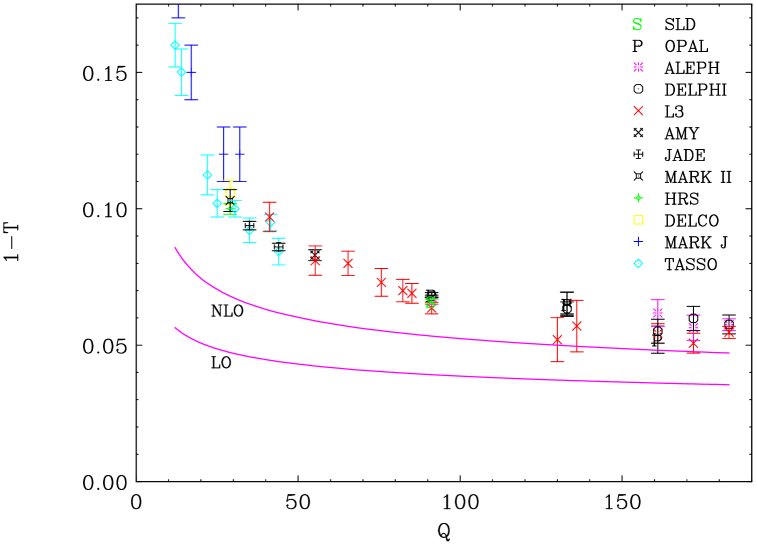
Figure 1: Average of $1-{\rm thrust}$ as a function of the center of mass energy Q, according to the available experimental data [52] and the leading order (LO) and next-to-leading order (NLO) perturbative QCD calculation in the $\overline{\rm MS}$ scheme with $\mu_{R}=Q$, given $\alpha_{s}^{\hbox{$\overline{\hbox{\tiny MS}}\,$}}({\rm M_{Z}})=0.117$.

There are theoretical indications that perturbative corrections at the next-to-next-to-leading order and beyond are large: the next-to-leading order term is quite a significant correction with respect to the leading order and there is a large renormalization scale dependence. However, the usual explanation of the discrepancy between the data and the next-to-leading order calculation is that hadronization related power corrections are important. It is intuitively clear from the definition of the thrust that emission of soft gluons implies a change in the thrust which is linear in the gluon momentum, and thus power like effects that fall as $1/Q$ can appear. Fits to the experimental data [3] confirm the existence of $1/Q$ power corrections. Event shape variables are quite special in having such strong power corrections: other QCD observables, like the ones for which higher twist terms can be analyzed using an operator product expansion, usually have power corrections that fall as $1/Q^{2}$ or faster.

Traditionally, extraction of $\alpha_{s}$ from experimental data is based on Monte-Carlo simulations that effectively generate “hadronization” power corrections, which are added to the next-to-leading order perturbative expression (135). In the last 5 years there have been several theoretical attempts to understand better the subject of power corrections in event shape variables. These includes analysis of the interplay between renormalons and power corrections [4, 5, 6, 9] and renormalon inspired approaches to parametrize power corrections, based on either a universal infrared regular physical coupling [7, 8] or a less restrictive observable-dependent non-perturbative shape function [10].

Since the average thrust is a priori expected to have both large perturbative corrections and significant power-like corrections, we find this observable quite appropriate to serve as an example of our approach.

5.1 The characteristic function for the average thrust

The observable dependent ingredient in the renormalon resummation program is the characteristic function ${\cal F}_{R}(\mu^{2}/Q^{2})$, which is defined by the leading order perturbative result for a gluon of mass $\mu^{2}$. In this section we shall calculate the characteristic function for the average thrust, ${\cal F}_{T}(\mu^{2}/Q^{2})$.

As mentioned in sec. 3, Minkowskian quantities usually have two different analytic functions: ${\cal F}^{(-)}(\epsilon)$ for $\epsilon\equiv\mu^{2}/Q^{2}<1$ and ${\cal F}^{(+)}(\epsilon)$ for $\epsilon>1$. The reason is that the former includes both real and virtual gluon diagrams while the latter includes only virtual gluon diagrams. In case of event shape variables like the thrust, virtual corrections do not contribute at one-loop, and so ${\cal F}_{T}^{(+)}(\epsilon)=0$. What remains to calculate is ${\cal F}_{T}^{(-)}(\epsilon)$ which is entirely due to real gluon emission. Let us simplify the notation and define ${\cal F}(\epsilon)\equiv{\cal F}^{(-)}_{T}(\epsilon)$. The “gluon mass” integral (18) is now performed up to $\mu^{2}=Q^{2}$

$$R_{\hbox{\tiny APT}}(Q^{2})=\int_{0}^{1}{d\epsilon\over\epsilon}\ \bar{a}^{\hbox{\tiny PT}}_{\hbox{\tiny eff}}(\epsilon Q^{2})\ \dot{{\cal F}}(\epsilon)$$ (137)

which implies that there are strictly no ultraviolet renormalons in this case: the large order behavior of $R_{\hbox{\tiny APT}}(Q^{2})$ when expanded in some scheme is determined just by the leading non-analytic terms in the small $\epsilon$ expansion of ${\cal F}(\epsilon)$, which are the leading infrared renormalons. The absence of ultraviolet renormalons is a direct consequence of the absence of virtual corrections at the order considered. Higher terms in the “skeleton expansion” may give rise to ultraviolet renormalons in the full perturbative series of $\left<t\right>$.

The characteristic function ${\cal F}(\epsilon)$ was calculated numerically in [8], and its leading term in the small $\epsilon$ expansion was obtained there analytically, ${\dot{\cal F}}(\epsilon)=4\sqrt{\epsilon}$, which indeed indicates $1/Q$ corrections. We shall repeat the calculation here. We find it important to have, if not an analytic expression for ${\cal F}(\epsilon)$, then at least several leading terms in its asymptotic expansion for small $\epsilon$. The sub-leading terms are required to verify the convergence of the power correction series (we shall see that in practice only $1/Q$ terms are important).

In order to explain how ${\cal F}(\epsilon)$ is computed we first briefly review the kinematics and the calculation of the thrust for three partons in the final state. Let us denote the primary photon 4-momentum by $Q$, the 4-momenta of the quark and anti-quark by $p_{1}$ and $p_{2}$ ($p_{i}^{2}=0$), and the 4-momenta of the “massive gluon” by $p_{3}$ ($p_{3}^{2}=\mu^{2}=\epsilon Q^{2}$). Following [2] we define $y_{ij}\equiv(p_{i}+p_{j})^{2}/Q^{2}$, which implies $y_{ij}>0$, and $x_{i}\equiv{2Q\cdot p_{i}}/{Q^{2}}$.

It follows from energy-momentum conservation that

$$x_{1}+x_{2}+x_{3}=2$$ (138)

and from the assumed virtualities of the particles that

$$y_{12}+x_{3}-\epsilon = 1$$

$$y_{13}+x_{2} = 1$$

$$y_{23}+x_{1} = 1.$$ (139)

In the center of mass frame, where $Q=(Q,0,0,0)$, $x_{i}$ becomes the energy fraction of the $i$ parton, $x_{i}\,=\,\frac{2}{Q}E_{i}$. It then follows that

$$\left|\vec{p}_{i}\right| = \frac{Q}{2}x_{i}\,\,\,\,\,\,\,\,\,\,\,\,\,\,\,\,\,\,\,\,\,\,\,\,\,\,\,i=1,2$$

$$\left|\vec{p}_{3}\right| = \frac{Q}{2}\sqrt{x_{3}^{2}-4\epsilon}.$$ (140)

The phase space limitations are the following:

a) Hard gluon limit,

$$x_{1}+x_{2}\geq 1-\epsilon,$$ (141)

which follows from the condition $y_{12}>0$ together with (138) and (5.1).

b) Soft gluon limit,

$$(1-x_{1})(1-x_{2})\geq\epsilon,$$ (142)

which is obtained in the center of mass frame, using (5.1), from the condition $|\vec{p}_{2}|=|\vec{p}_{1}+\vec{p}_{3}|\leq|\vec{p}_{1}|+|\vec{p}_{3}|$.

The phase space limitations are shown in fig. 2 for the case $\epsilon=0.1$.

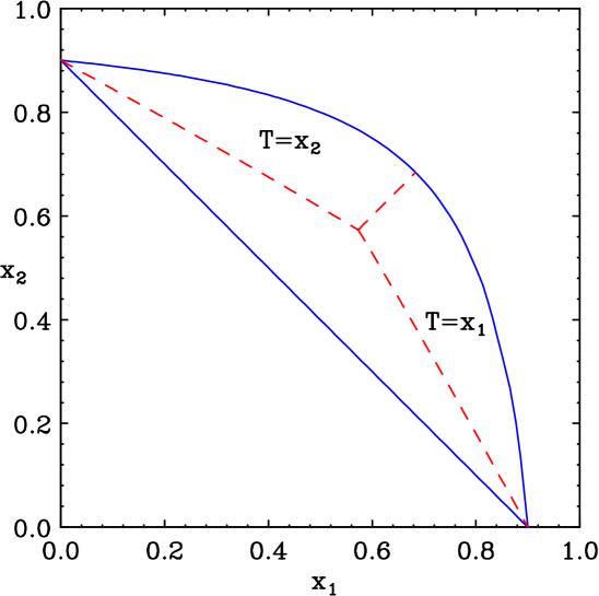
Figure 2: Phase-space for the emission of a virtual gluon with $\mu^{2}\,=\,\epsilon\,Q^{2}\,=\,0.1\,Q^{2}$ in the plane of the quark and anti-quark energy fractions ($x_{1,2}$). Continuous lines represent phase-space limits: the upper (curved) line corresponds to the softest gluons (142) while the lower (linear) line corresponds to the hardest (141). Dashed lines represent the separation of phase-space according to which particle carries the largest momentum and thus determines the thrust axis (cf. eq. (146)): in the upper left region $T=x_{2}$, in the upper right region $T=x_{1}$ and in the lower region $T=\sqrt{x_{3}^{2}-4\epsilon}$.

The region near the outer (curved) line corresponding to (142) represents soft gluons: for a given “gluon mass” $\epsilon Q^{2}$ and quark energy fraction ($x_{1}$), the smallest possible gluon energy is obtained when the inequality (142) is saturated. The region near the inner (linear) line corresponding to (141) represents hard gluons with maximal energy $x_{3}=1+\epsilon$. Note that as $\epsilon$ increases the relevant phase space shrinks and approaches the region of small $x_{1}$ and $x_{2}$ (the lower left corner in fig. 2).

The characteristic function ${\cal F}(\epsilon)$ is obtained from the following integral over phase space [8],

$${\cal F}(\epsilon)=\int_{\rm\tiny{phase\,\,space}}dx_{1}dx_{2}\,{\cal M}(x_{1},x_{2},\epsilon)\,t(x_{1},x_{2},\epsilon),$$ (143)

where $\frac{C_{F}}{2}\,{\cal M}\,a$ is the squared tree level matrix element for the production of a quark, an anti-quark and a gluon of “mass” $\mu^{2}=\epsilon Q^{2}$ and

$${\cal M}(x_{1},x_{2},\epsilon)=\frac{(x_{1}+\epsilon)^{2}+(x_{2}+\epsilon)^{2}}{(1-x_{1})(1-x_{2})}-\frac{\epsilon}{(1-x_{1})^{2}}-\frac{\epsilon}{(1-x_{2})^{2}}.$$ (144)

The last ingredient for the calculation of ${\cal F}(\epsilon)$ is the expression for the thrust. For two particles in the final state, the thrust axis $\vec{n}_{T}$ coincides with the line along which they move and $T=1$. For three particles in the final state, it coincides with the direction of the particle carrying the largest momentum, $|\vec{p}_{i}|$. By momentum conservation in the center of mass frame, the two other particles have the sum of momenta $\vec{p}_{j}+\vec{p}_{k}=-\vec{p}_{i}$. The numerator in (134) then equals $2|\vec{p}_{i}|$. For three massless particles the denominator in (134) equals $|\vec{p}_{1}|+|\vec{p}_{2}|+|\vec{p}_{3}|=E_{1}+E_{2}+E_{3}=Q$. Thus, using (5.1), we have $T=x_{i}$. For a massive gluon, however, the denominator is $\frac{Q}{2}(x_{1}+x_{2}+\sqrt{x_{3}^{2}-4\epsilon})\,\neq\,Q$. On the other hand, since the “massive gluon” dissociates into massless partons one should actually calculate the thrust taking into account the final partons. In this case the denominator is $Q$. Note that the numerator remains the same whether or not one takes into account the gluon dissociation, provided that all the partons produced end up in the same hemisphere as the parent gluon – an assumption to which we return below. In conclusion we find that, due to the change in the denominator of (134), by giving mass to the gluon (in order to represent its dissociation through the dispersive approach) we unwillingly change the calculated value of the thrust. To solve this difficulty it has been suggested [8] to modify the definition of the thrust such that the normalization will be with respect to the sum of energies ($Q$),

$$T=\frac{\sum_{i}\left|\vec{p}_{i}\cdot\vec{n}_{T}\right|}{\sum_{i}E_{i}}=\frac{\sum_{i}\left|\vec{p}_{i}\cdot\vec{n}_{T}\right|}{Q}.$$ (145)

There is no difference between (145) and (134) so long as only massless particles are produced. However, for the theoretical computation with a “massive gluon” it is important to use (145) which guarantees that the same value of the thrust is obtained with a “massive gluon” as with the massless products of its dissociation. The final result for the thrust, using (145), is

$$t(x_{1},x_{2},\epsilon)={\rm min}\left\{1-x_{1}\,,\,1-x_{2}\,,\,1-\sqrt{(2-x_{1}-x_{2})^{2}-4\epsilon}\right\}.$$ (146)

Fig. 2 shows the separation of phase space to regions where each of the three particles has the largest momentum and thus determines the thrust axis.

Let us now return to the more delicate problem, namely the assumption we made concerning the decay products of the gluon. This assumption is absolutely necessary in order to keep the same value of the thrust when referring to the “massive gluon” itself as when referring to the massless products of its dissociation. In the first case the relevant term in the numerator of (145) is $|\vec{p}_{3}\cdot\vec{n}_{T}|$ while in the second it is larger: $|\vec{p_{L}}\cdot\vec{n}_{T}|+|\vec{p_{R}}\cdot\vec{n}_{T}|$, where $\vec{p}_{3}=\vec{p}_{L}+\vec{p}_{R}$ and $\vec{p}_{L}$ ($\vec{p}_{R}$) corresponds to the sum of momenta of the particles that originate in the gluon and end up in the left (right) hemisphere. It is a priori not clear whether this assumption is justified: kinematic considerations alone do not exclude the possibility of dissociation into opposite hemispheres and in fact when the gluon is close to the transverse direction, it is quite plausible that it would dissociate this way. The “massive gluon” approach is justified [24, 25, 8] for completely inclusive quantities: then dressing the gluon or taking into account its dissociation amounts exactly to building up the running coupling. We see that the thrust is not inclusive enough. We can still ask, however, how large is the error we introduce using the inclusive “massive gluon” approach instead of taking into account separately the contribution of the decay products of the gluon. The problem of non-inclusiveness was first raised in [5] in the framework of renormalon resummation in the large $N_{f}$ limit where the terms which prohibit an inclusive treatment were identified and evaluated. We shall return to this issue in the next section.

Let us now proceed with the calculation of ${\cal F}(\epsilon)$ for the thrust, based on the definition (143), the squared matrix element (144) the expression for the thrust (146) and the phase space limitations (141) and (142) which determine the integration range. In order to evaluate the integral (143) one has to treat separately each of the three regions of phase space (see fig. 2): the integrand in each of them is different, as implied by (146). To perform the integrals it is useful to change the integration variables to the following: $z_{1}=x_{1}+x_{2}+\epsilon-1$ and $z_{2}=x_{1}-x_{2}$, which fit better the phase space limitations. Most eventual integrals can be performed analytically but the resulting functions are complicated. Instead, we calculated the integral numerically for any $0<\epsilon<1$ and in addition obtained an asymptotic expansion of ${\cal F}(\epsilon)$ for small $\epsilon$,

$${\cal F}(\epsilon) = -{\frac{1}{18}}+\pi^{2}+8\,\rm{ln}(3)\,\rm{ln}(2)-{\frac{3}{4}}\,\rm{ln}(3)+4\,\rm{dilog}(4)+4\,\rm{dilog}(3)$$

$$- 8\,\epsilon^{\frac{1}{2}}+\left[4+12\,\rm{ln}(3)\right]\,\epsilon-{\frac{160}{9}}\,\epsilon^{\frac{3}{2}}$$

$$+ \left[-3\,\rm{ln}\left({\frac{1}{\epsilon}}\right)+{\frac{17}{6}}-\pi^{2}-8\,\rm{ln}(3)\,\rm{ln}(2)-4\,\rm{dilog}(4)+{\frac{56}{3}}\,\rm{ln}(2)-4\,\rm{dilog}(3)\right]\,\epsilon^{2}$$

$$- 8\,\epsilon^{\frac{5}{2}}+\left[{\frac{28}{15}}\,\rm{ln}(2)-{\frac{8}{5}}+{\frac{16}{3}}\,\rm{ln}\left({\frac{1}{\epsilon}}\right)\right]\,\epsilon^{3}$$

$$+ \left[-11\,\rm{ln}\left({\frac{1}{\epsilon}}\right)+{\frac{2719}{630}}-{\frac{128}{105}}\,\rm{ln}(2)\right]\,\epsilon^{4}+\,\cdots$$

$$= 1.5776-8\,\epsilon^{\frac{1}{2}}+17.1833\,\epsilon-17.7778\,\epsilon^{\frac{3}{2}}+\left[-3\,\rm{ln}\left({\frac{1}{\epsilon}}\right)+13.3149\right]\,\epsilon^{2}$$

$$- 8\,\epsilon^{\frac{5}{2}}+\left[-0.3061+5.3333\,\rm{ln}\left({\frac{1}{\epsilon}}\right)\right]\,\epsilon^{3}+\left[-11\,\rm{ln}\left({\frac{1}{\epsilon}}\right)+3.4709\right]\,\epsilon^{4}+\,\cdots$$

The agreement between the asymptotic expansion (5.1) and the numerical calculation is shown in fig. 3.

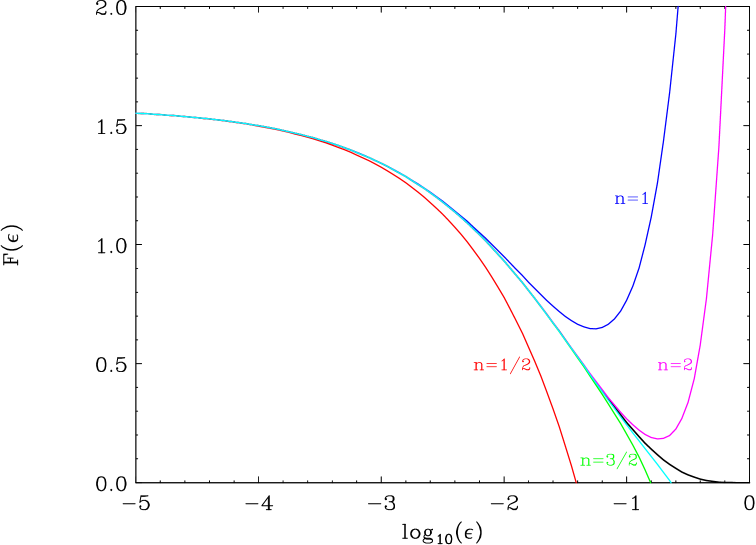
Figure 3: The characteristic function ${\cal F}(\epsilon)$ for the average thrust (143) as a function of $\log_{10}(\epsilon)$, where $\mu^{2}=\epsilon Q^{2}$ is the “gluon mass”. ${\cal F}(\epsilon)$ is represented by a thick black line reaching zero in the limit $\epsilon\longrightarrow 1$. It is compared with its asymptotic expansion at small $\epsilon$ (5.1), for $n=\frac{1}{2},1,\frac{3}{2},2,\frac{5}{2}$, where $n$ is the highest order term ${\cal O}(\epsilon^{n})$ taken into account in each approximating curve.

As we saw in the previous sections, the leading terms in the small $\epsilon$ expansion of ${\cal F}(\epsilon)$ are required for the calculation of the difference between different regularizations of the perturbative sum and eventually for the parametrization of power corrections. Each term in eq. (5.1) has the form of eq. (43) and so the numerical coefficients $B_{T}^{(n)}$ and $C_{T}^{(n)}$ can be immediately identified. The first non-analytic term in (5.1) is a square root one, corresponding to a 1/Q infrared power correction. The coefficient of this term agrees with previous calculations [8]: $\dot{\cal F}(\epsilon)=4\sqrt{\epsilon}$. As explained there, this term arises from the limit of phase space (142) corresponding to the softest gluons.

A new observation is that there are no $1/Q^{2}$ infrared power corrections in this “leading skeleton” approximation. The next non-analytic term in (5.1) is $\epsilon^{\frac{3}{2}}$ associated with $1/Q^{3}$ infrared power corrections. As a result the apparent convergence of the discontinuity function $\Phi(k^{2}/Q^{2})$

$$\Phi(k^{2}/Q^{2})\simeq\,\frac{1}{\pi}\,\left(\frac{k^{2}}{Q^{2}}\right)^{\frac{1}{2}}\left[8-17.7778\left(\frac{k^{2}}{Q^{2}}\right)+\cdots\right]$$ (148)

is better than that of ${\cal F}(\epsilon)$. In (148) the second term becomes about $20\%$ of the first around $k^{2}\,\sim\,0.1\,Q^{2}$. Another observation is that the asymptotic expansion (5.1) does not contain double logarithmic terms up to the order considered.

Finally, taking the logarithmic derivative we obtain $\dot{\cal F}(\epsilon)=-\epsilon\,d{\cal F}/d\epsilon$, which agrees with the numerical results of [8]. In fig. 4 one can see that there is just a small contribution to the characteristic function, and thus also to the value of the average thrust, from the kinematic configurations where the gluon momentum is the largest. Moreover, this contribution to $\dot{\cal F}(\epsilon)$ has some significance only for fairly large “gluon mass” $\epsilon\mathrel{\mathchoice{\vbox{\offinterlineskip\halign{$\m@th\displaystyle\hfil#\hfil$\cr>\crcr\sim\crcr} }}{\vbox{\offinterlineskip\halign{$\m@th\textstyle\hfil#\hfil$\cr>\crcr\sim\crcr} }}{\vbox{\offinterlineskip\halign{$\m@th\scriptstyle\hfil#\hfil$\cr>\crcr\sim\crcr} }}{\vbox{\offinterlineskip\halign{$\m@th\scriptscriptstyle\hfil#\hfil$\cr>\crcr\sim\crcr} }}}10^{-2}$, and so its effect on the large order behavior of the perturbative series and the related power corrections is negligible.

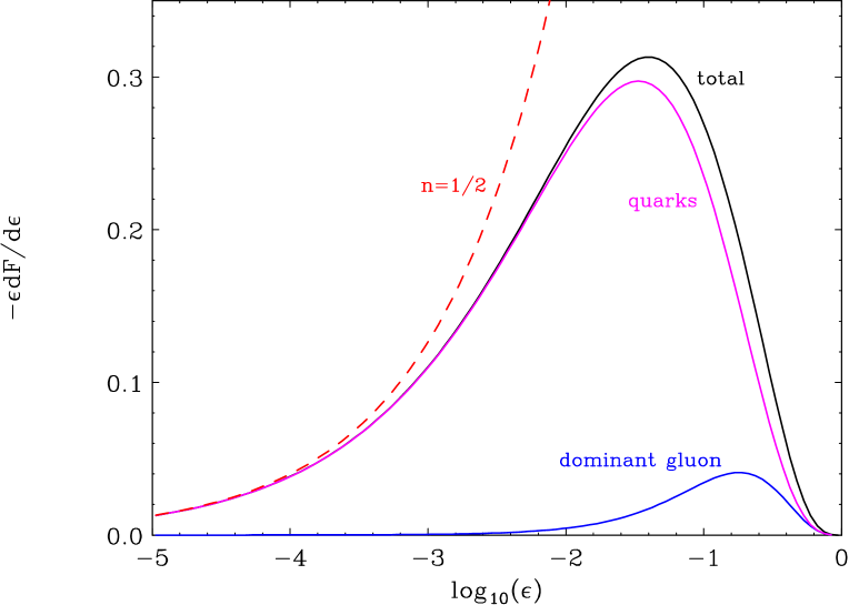
Figure 4: The derivative of the characteristic function for the average thrust $\dot{{\cal F}}(\epsilon)$ as a function of $\log_{10}(\epsilon)$, where $\mu^{2}=\epsilon Q^{2}$ is the “gluon mass”. The separate contributions from kinematic configurations where one of the quarks or the gluon carries the largest momentum are shown as well. The dashed line represents the leading ($n=\frac{1}{2}$) term in the small $\epsilon$ expansion of this function, $\dot{{\cal F}}(\epsilon)\simeq 4\sqrt{\epsilon}$.

5.2 Does the renormalon resummation program apply to non-inclusive quantities?

The “skeleton expansion” approach and thus our renormalon resummation program are based on the assumption that all the higher order diagrams related to the running of the coupling contribute inclusively to the observable. This assumption does not hold in the case of event shape variables like thrust. In the previous section we calculated the thrust characteristic function using a “massive gluon”, which should represent after integration with respect to the discontinuity of the running coupling, the partons to which the gluon dissociates. We encountered and eventually ignored the non-inclusive nature of the thrust: as explained there, if the decay products of the gluon end up in different hemispheres the average thrust value obtained in the “massive gluon” calculation is different (and in fact always lower) than it is in reality. Still, we intuitively expect that most decays are roughly collinear and so for the major part of the phase space decay into opposite hemispheres is not very likely. We therefore conjecture that the inclusive resummation approach can provide a reasonable approximation to the full higher order corrections. In the following we give a quantitative argument at the next-to-leading order level in favor of this conjecture.

In order to estimate the error we are making by the inclusive treatment, let us compare the two type of expansions we have: the ordinary perturbative expansion, e.g. eq. (135) in the ${\rm\overline{MS}}$ scheme, and the conjectured “skeleton expansion”, i.e. the equivalent of (4) and (17) for the average thrust

$$\left<t\right>_{\hbox{\tiny PT}}(Q^{2})\,=\,\frac{C_{F}}{2}\,\left[\left(S_{0}^{\hbox{\tiny PT}}(Q^{2})+S_{1}^{\hbox{\tiny PT}}(Q^{2})+\cdots\right)+{\rm Non-Skeleton}\right]$$ (149)

where similarly to $R_{i}^{\hbox{\tiny PT}}$ in eq. (17) $S_{0}^{\hbox{\tiny PT}}$ is the leading “dressed skeleton” term, normalized as $S_{0}^{\hbox{\tiny PT}}=t_{0}\,a+{\cal O}(a^{2})$, $S_{1}^{\hbox{\tiny PT}}$ is the second “dressed skeleton” term which starts at order $a^{2}$ and so on. The ${\rm Non-Skeleton}$ piece allows for additional perturbative terms of order $a^{2}$ or higher which do not fit into a “skeleton expansion” due to the non-inclusive nature of the observable. The “leading skeleton” term $S_{0}^{\hbox{\tiny PT}}$ is given by $R_{\hbox{\tiny APT}}$ of eq. (18), up to a regularization related power term which we now ignore. Since both $S_{1}^{\hbox{\tiny PT}}$ and the ${\rm Non-Skeleton}$ terms start at order $a^{2}$, we can approximate $\left<t\right>_{\hbox{\tiny PT}}(Q^{2})$ by

$$\left<t\right>_{\hbox{\tiny PT}}(Q^{2})\,\simeq\,\frac{C_{F}}{2}\,\left[S_{0}^{\hbox{\tiny PT}}(Q^{2})+\delta_{\hbox{\tiny NLO}}\right]$$ (150)

with

$$\delta_{\hbox{\tiny NLO}}=\tilde{t}_{1}a^{2}\,+\,\cdots$$ (151)

where in general the coefficient $\tilde{t}_{1}$ contains contributions from both $S_{1}^{\hbox{\tiny PT}}$ and the ${\rm Non-Skeleton}$ terms. To compare the two expansions, let us expand the time-like coupling within the first “skeleton” term $R_{\hbox{\tiny APT}}$ (18) in terms of $a_{\hbox{$\overline{\hbox{\tiny MS}}\,$}}$. Note that at a difference with sec. 2, it is the Minkowskian representation that we start with. Taking the one-loop form (21) of the coupling we obtain from (22) the following expansion in $a_{\hbox{$\overline{\hbox{\tiny MS}}\,$}}(Q^{2})$

$$\bar{a}^{\hbox{\tiny PT}}_{\hbox{\tiny eff}}(\mu^{2})=a_{\hbox{$\overline{\hbox{\tiny MS}}\,$}}(Q^{2})\,+\,\left\{d_{1}-\left(c_{1}+\log\frac{\mu^{2}}{Q^{2}}\right)\beta_{0}\right\}\,a_{\hbox{$\overline{\hbox{\tiny MS}}\,$}}^{2}(Q^{2})\,\,+$$

$$\left\{{d_{1}}^{2}\,-\,2{d_{1}}\,\left({c_{1}}+\log\frac{\mu^{2}}{Q^{2}}\right)\beta_{0}\,+\,\left[\left({c_{1}}+\log\frac{\mu^{2}}{Q^{2}}\right)^{2}-{\frac{1}{3}}\,\pi^{2}\right]\beta_{0}^{2}\right\}a_{\hbox{$\overline{\hbox{\tiny MS}}\,$}}^{3}(Q^{2})+\cdots$$

where the first two terms are actually valid beyond the one-loop approximation of the coupling and also coincide with the corresponding terms in the expansion of the space-like coupling (7). Inserting (5.2) into (18) yields

$$S_{0}^{\hbox{\tiny PT}}(Q^{2})=t_{0}\,a_{\hbox{$\overline{\hbox{\tiny MS}}\,$}}(Q^{2})\,+\,t_{1}^{0}\,a_{\hbox{$\overline{\hbox{\tiny MS}}\,$}}^{2}(Q^{2})\,\,+t_{2}^{0}\,a_{\hbox{$\overline{\hbox{\tiny MS}}\,$}}^{3}(Q^{2})\,+\,\cdots$$

with

$$t_{0} = f_{0}$$ (153)

$$t_{1}^{0} = {d_{1}}\,{f_{0}}-({c_{1}}\,{f_{0}}+{f_{1}})\,\beta_{0}$$

$$t_{2}^{0} = {d_{1}}^{2}\,{f_{0}}\,-\,2\,{d_{1}}\,({c_{1}}\,{f_{0}}+{f_{1}})\,\beta_{0}+\left[\left({c_{1}}^{2}-{\frac{1}{3}}\,\pi^{2}\right)\,{f_{0}}+2\,{c_{1}}\,{f_{1}}+{f_{2}}\right]\,\beta_{0}^{2}$$

and so on. Note that at the next-to-next-to-leading order ($t_{2}^{0}$) we recover the characteristic $\pi^{2}$ terms which appear in perturbative expansions of Minkowskian observables. The constants $f_{i}$ are the log-moments of the characteristic function (compare with (10))

$$f_{i}\equiv\int_{0}^{\infty}{d\mu^{2}\over\mu^{2}}\ \left(\log{\mu^{2}\over Q^{2}}\right)^{i}\ \dot{\cal F}(\mu^{2}/Q^{2}).$$ (154)

Using the numerical result for the characteristic function of the average thrust one can obtain $f_{i}$ to any arbitrary order. The first values are

$$f_{0} = 1.577602558$$

$$f_{1} = -7.176762311$$

$$f_{2} = 42.11235577$$

$$f_{3} = -307.991760$$

$$f_{4} = 2736.14010$$

$$f_{5} = -28923.5429$$

$$f_{6} = 357358.9993$$ (155)

With these coefficients at hand one can construct a power series approximation (5.2) to the first “skeleton” term $S_{0}^{\hbox{\tiny PT}}$ of eq. (18) to any arbitrary order, provided one specifies the “skeleton coupling” $\overline{a}_{\hbox{\tiny PT}}$, namely the parameters $d_{1}$ and $c_{1}$. As discussed at the end of sec. 2, we use in this work several different schemes for the “skeleton coupling” $\overline{a}_{\hbox{\tiny PT}}$. In the Abelian limit, $\overline{a}_{\hbox{\tiny PT}}$ should coincide with the V-scheme coupling and so $c_{1}=-\frac{5}{3}$. We can thus determine the $\beta_{0}$ dependent piece in $t_{1}^{0}$ in eq. (153)

$$-(c_{1}f_{0}+f_{1})\,\beta_{0}=9.8061\,\beta_{0}.$$ (156)

We now have all the ingredients for the comparison up to next-to-leading order between the “skeleton expansion” (150) and the standard expansion (135). For the first we use (5.2) and obtain

$$\left<t\right>_{\hbox{\tiny PT}} = \,\frac{C_{F}}{2}\,\left\{t_{0}\,a_{\hbox{$\overline{\hbox{\tiny MS}}\,$}}(Q^{2})+\left(\tilde{t}_{1}+t_{1}^{0}\right)\,a_{\hbox{$\overline{\hbox{\tiny MS}}\,$}}^{2}(Q^{2})+{\cal O}\left(a_{\hbox{$\overline{\hbox{\tiny MS}}\,$}}^{3}(Q^{2})\right)\right\}$$

$$= \,\frac{C_{F}}{2}\,\left\{{f_{0}\,a_{\hbox{$\overline{\hbox{\tiny MS}}\,$}}(Q^{2})+\left[\tilde{t}_{1}+{d_{1}}\,{f_{0}}-({c_{1}}\,{f_{0}}+{f_{1}})\,\beta_{0}\right]\,a_{\hbox{$\overline{\hbox{\tiny MS}}\,$}}^{2}(Q^{2})}+{\cal O}\left(a_{\hbox{$\overline{\hbox{\tiny MS}}\,$}}^{3}(Q^{2})\right)\right\}$$

By construction the leading order is the same. The comparison at the next-to-leading order gives

$$\tilde{t}_{1}+{d_{1}}\,{f_{0}}+9.8061\,\beta_{0}\,=\,-4.128+10.134\,\beta_{0}$$ (158)

where the l.h.s. corresponds to the “skeleton expansion” coefficients $\tilde{t}_{1}+t_{1}^{0}$ of eq. (5.2) and the r.h.s. to the standard expansion coefficient $t_{1}$ of eq. (136), with the $N_{f}$ dependence expressed in terms of $\beta_{0}$ (3).

For an inclusive quantity, where we assume that the “skeleton expansion” exists (i.e. the ${\rm Non-Skeleton}$ terms in (149) are absent), the $N_{f}$ dependence at the next-to-leading order comes only from diagrams that are related to the running of the coupling. In such a case the entire $\beta_{0}$ dependent piece in the next-to-leading order coefficient is accounted for by the leading term $S_{0}^{\hbox{\tiny PT}}$ in the “skeleton expansion”, and the remaining coefficient $\tilde{t}_{1}$ in (150), which coincides now with the normalization of the sub-leading “skeleton” $S_{1}^{\hbox{\tiny PT}}=\tilde{t}_{1}a^{2}+\cdots$, should be free of $\beta_{0}$. For the thrust, which is non-inclusive with respect to the decay products of the gluon, this does not hold. However, we find that the difference between the term linear in $\beta_{0}$ in (5.2) $9.8061\,\beta_{0}$ (l.h.s. in (158)) and in full next-to-leading QCD coefficient $10.134\,\beta_{0}$ (r.h.s. in (158)) is quite small: it is about 3 percent. This finding gives place to hope that the ${\rm Non-Skeleton}$ terms in (149) are small and thus the inclusive treatment is after all a good approximation for the resummation of a certain class of diagrams.

The observation that for a non-inclusive quantity the $N_{f}$ dependence of the next-to-leading order coefficient cannot be explained in terms of the running coupling also implies that the usual motivation for BLM scale fixing and the Naive Non-Abelianization procedure does not hold. As opposed to the inclusive case discussed in sec. 2, the BLM scale computed from the full next-to-leading order coefficient does not coincide with the one of the “leading skeleton”. As a result, the identification made following eq. (13), between the remaining next-to-leading order coefficient and the BLM coefficient in the “skeleton scheme” fails: the former still contains some $N_{f}$ dependence while the latter does not. Like our resummation program, the BLM procedure becomes relevant once the observation is made that the $\beta_{0}$ dependent terms in the two sides of eq. (158) are numerically very close.

Finally, using (158) we evaluate $\tilde{t}_{1}$. If the coupling $\overline{a}_{\hbox{\tiny eff}}^{\hbox{\tiny PT}}$ in the “leading skeleton” term (18) is the time-like coupling associated (20) with the “gluon bremsstrahlung” coupling [30] (see the end of sec. 2), where $d_{1}^{\hbox{\tiny brem}}=1-{\pi^{2}\over 4}$, then

$$\tilde{t}_{1}^{\hbox{\tiny brem}}=-1.813+0.328\,\beta_{0}.$$ (159)

For the pinch technique coupling [22] $d_{1}^{\hbox{\tiny pinch}}=1$, and so

$$\tilde{t}_{1}^{\hbox{\tiny pinch}}=-5.706+0.328\,\beta_{0}.$$ (160)

For the V-scheme coupling [15], $d_{1}^{\hbox{\tiny V}}=-2$, and then

$$\tilde{t}_{1}^{\hbox{\tiny V}}=-0.973+0.328\,\beta_{0}.$$ (161)

For $N_{f}=5$ the coefficients are $\tilde{t}_{1}^{\hbox{\tiny brem}}=-1.184$, $\tilde{t}_{1}^{\hbox{\tiny pinch}}=-5.077$ and $\tilde{t}_{1}^{\hbox{\tiny V}}=-0.344$. These coefficients can be compared with the standard next-to-leading coefficient in ${\rm{\overline{MS}}}$ (136) which equals $t_{1}\simeq 15.296$. We conclude that at least the apparent convergence of the suggested expansion is better than that of the standard one. The coefficient is extremely small in the “gluon bremsstrahlung” and V schemes. We shall thus choose for our phenomenological analysis two couplings:

a) the “gluon bremsstrahlung” scheme which was used before in the analysis of power corrections to the thrust [7, 8]. This coupling will be quite convenient in practice: having a small next-to-leading coefficient (159), the full result should be close to the first term in the “skeleton expansion”.

b) the pinch technique coupling which may be the correct physical “skeleton coupling” $\bar{a}$. Using this coupling, with its relatively large next-to-leading coefficient (160), in addition to the “gluon bremsstrahlung” coupling, will be useful to measure the sensitivity of our procedure to the value of $d_{1}$.

5.3 The perturbative sum vs. experimental data

The most convenient way to calculate the perturbative sum is to use the APT formula (18). As explained in sec. 3, other regularizations of the perturbative sum, such as the principal value Borel sum can then be obtained from $R_{\hbox{\tiny APT}}$.

The ingredients required for the calculation of $R_{\hbox{\tiny APT}}$ are the numerical function ${\cal F}(\mu^{2}/Q^{2})-{\cal F}(0)$ we obtained in sec. 5.1 and the discontinuity of the perturbative coupling on the time-like axis, $\overline{\rho}_{\hbox{\tiny PT}}(\mu^{2})$. For the latter, we shall use here the one and two loop couplings. In the one-loop case (21), the expression obtained from (19) is simply

$$\overline{\rho}_{\hbox{\tiny 1-loop}}(\mu^{2})=-\frac{1}{\beta_{0}}\,\frac{1}{\pi^{2}+\log{\,{}^{2}}\left(\frac{\mu^{2}}{\Lambda^{2}}\right)}.$$ (162)

In the two-loop case we use the Lambert W function representation of the coupling [37, 38]

$$\begin{array}[]{c}\displaystyle\bar{a}_{\hbox{\tiny 2-loop}}(k^{2})=-\frac{\beta_{0}}{\beta_{1}}\,\,\frac{1}{1+W_{-1}(z)}\\ \phantom{a}\\ \displaystyle z=-\frac{1}{e}\left(\frac{k^{2}}{\Lambda^{2}}\right)^{-\beta_{0}^{2}/\beta_{1}}\end{array}$$

where $W(z)$ is the Lambert W function defined by $W(z)\exp\left[W(z)\right]=z$ and the particular branch $W_{-1}(z)$ is implied by asymptotic freedom: in the ultraviolet $z\longrightarrow 0^{-}$ and $W_{-1}(z)\longrightarrow-\infty$ [38]. Note that in (5.3) the explicit Landau pole and the tip of the branch cut coincide ($W_{-1}(-1/e)=-1$) and so there is only one singularity in the complex momentum plane, at $k^{2}=\Lambda^{2}$, with a cut $-\infty<k^{2}<\Lambda^{2}$. Using the computer algebra program Maple, $W_{-1}(z)$ is readily available at any given complex $z$. It is then straightforward to obtain the time-like discontinuity $\overline{\rho}_{\hbox{\tiny 2-loop}}(\mu^{2})$ (19) corresponding to $\bar{a}_{\hbox{\tiny 2-loop}}(k^{2})$.

As a first trial, let us calculate $R_{\hbox{\tiny APT}}$ based on the world average value of $\alpha_{s}$, $\alpha_{s}^{\hbox{$\overline{\hbox{\tiny MS}}\,$}}({\rm M_{Z}})=0.117$. We choose $\bar{a}_{\hbox{\tiny PT}}$ in the “gluon bremsstrahlung” scheme. Taking $N_{f}=5$ we find $\Lambda_{\hbox{\tiny brem}}^{\hbox{\tiny 1-loop}}=0.130\,{\rm GeV}$ and $\Lambda_{\hbox{\tiny brem}}^{\hbox{\tiny 2-loop}}=0.361\,{\rm GeV}$. We evaluate the perturbative sum $R_{\hbox{\tiny APT}}(Q^{2})$ in (18) by a numerical integration of ${\cal F}(\mu^{2}/Q^{2})-{\cal F}(0)$ times either $\overline{\rho}_{\hbox{\tiny 1-loop}}(\mu^{2})$ or $\overline{\rho}_{\hbox{\tiny 2-loop}}(\mu^{2})$.

Next, we use $R_{\hbox{\tiny APT}}$ to calculate the principal value Borel sum, according to $R_{\hbox{\tiny PT}|\hbox{\tiny PV}}=R_{\hbox{\tiny APT}}-{\rm Re}\left\{\delta R_{\hbox{\tiny APT}}\right\}$, where ${\rm Re}\left\{\delta R_{\hbox{\tiny APT}}\right\}$ is evaluated for a generic term in the small $\epsilon$ expansion of ${\cal F}(\epsilon)$ (5.1) by eq. (90) and (113) in the one and two loop cases, respectively. At order $n$ in the expansion, the contribution to ${\rm Re}\left\{\delta R_{\hbox{\tiny APT}}\right\}$ is ${\cal O}(1/Q^{2n})$. Since ${\rm Re}\left\{\delta R^{\hbox{\tiny APT}}_{\frac{1}{2}}\right\}$ in eq. (90) and (113) vanishes identically, the leading contribution is at order $n=1$. We note that the $n=1$ term in ${\cal F}(\epsilon)$ is analytic, and so this contribution is not of infrared origin. We obtain

$$\left.{\rm Re}\left\{\delta R_{\hbox{\tiny APT}}\right\}\right|_{\hbox{\tiny 1-loop}} = \frac{\Lambda^{2}_{\hbox{\tiny 1-loop}}}{Q^{2}}\,C_{T}^{(1)}\frac{1}{\beta_{0}}=8.96\,\frac{\Lambda^{2}_{\hbox{\tiny 1-loop}}}{Q^{2}}$$

$$\left.{\rm Re}\left\{\delta R_{\hbox{\tiny APT}}\right\}\right|_{\hbox{\tiny 2-loop}} = \frac{\Lambda^{2}_{\hbox{\tiny 2-loop}}}{Q^{2}}\,C_{T}^{(1)}\frac{1}{\beta_{0}}\,\Gamma(1+\delta_{1})\,\delta_{1}^{\delta_{1}}\,e^{-\delta_{1}}=3.18\,\frac{\Lambda^{2}_{\hbox{\tiny 2-loop}}}{Q^{2}}$$ (163)

where the numerical values were obtained using $\delta_{1}=\beta_{1}/\beta_{0}^{2}$ and $C_{T}^{(1)}=17.1833$. We find that ${\rm Re}\left\{\delta R_{\hbox{\tiny APT}}\right\}$ is absolutely negligible, already at the lowest relevant experimental value $Q=12\,{\rm GeV}$, where it is less than one percent of $R_{\hbox{\tiny APT}}$ (see table 5 in sec. 5.5).

The results for the average thrust $\left<t\right>_{\hbox{\tiny PT}}(Q^{2})\simeq\frac{C_{F}}{2}R_{\hbox{\tiny APT}}\simeq\frac{C_{F}}{2}R_{\hbox{\tiny PT}|\hbox{\tiny PV}}$ are shown in fig. 5 (within the resolution of the figure $R_{\hbox{\tiny APT}}$ and $R_{\hbox{\tiny PT}|\hbox{\tiny PV}}$ could hardly be distinguished). The first observation is that the difference between the one-loop and two-loop resummation results is quite small. This stability, which shall be discussed further in sec. 5.6, is reassuring since in our approach $\bar{a}_{\hbox{\tiny PT}}$ should actually be an all-order running coupling, and so its replacement by the one-loop coupling at all scales is not obviously justified, as already noted in sec. 3.3.

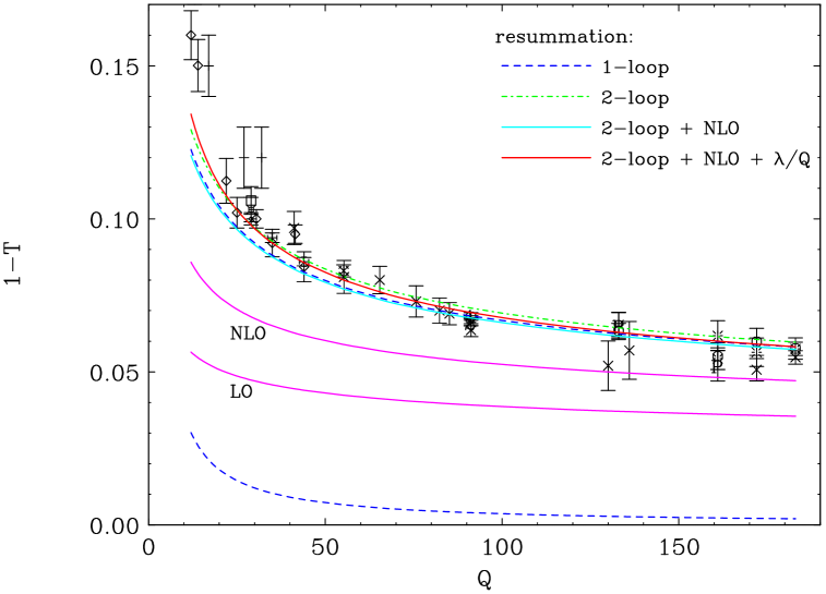
Figure 5: Average of $1-{\rm thrust}$ as a function of Q: experimental data is compared with naive perturbative QCD results (LO and NLO in $\overline{\rm MS}$ with $\mu_{R}=Q$) and with the resummed perturbative series in the APT or principal value Borel sum regularizations (the two coincide). All the theoretical calculations are based on $\alpha_{s}^{\hbox{$\overline{\hbox{\tiny MS}}\,$}}({\rm M_{Z}})=0.117$. Both one-loop (upper dashed) and two-loop (dot-dash) resummation results ($R_{\hbox{\tiny APT}}$) are presented, where the running coupling $\bar{a}_{\hbox{\tiny PT}}$ is in the “gluon bremsstrahlung” scheme. In the two-loop case we also show eq. (165) (lower continuous line; just below the upper dashed line) which includes the full ${\cal O}(\alpha_{s}^{2})$ term and eq. (166) (upper continuous line) which includes in addition a fitted $\lambda/Q$ term. The lower dashed line is the absolute value of the imaginary part of the one-loop Borel sum, which reflects the magnitude of the renormalon ambiguity.

In order to compare our results with experimental data, we should include the estimated contribution of the terms not included in the “leading skeleton” according to eqs. (150) and (151). For a concrete estimate of $\delta_{\hbox{\tiny NLO}}$ we replace the arbitrary scheme coupling $a$ by the natural effective charge at hand, namely the value of the “leading skeleton” with the appropriate normalization

$$\delta_{\hbox{\tiny NLO}}=\tilde{t}_{1}a^{2}\simeq\tilde{t}_{1}\left(\frac{R_{\hbox{\tiny APT}}}{f_{0}}\right)^{2}$$ (164)

and thus

$$\left<t\right>_{\hbox{\tiny PT}}=\frac{C_{F}}{2}\left[R_{\hbox{\tiny APT}}+\tilde{t}_{1}\left(\frac{R_{\hbox{\tiny APT}}}{f_{0}}\right)^{2}\right].$$ (165)

This expression exhausts our knowledge concerning the perturbative contribution to the average thrust, as it includes, in addition to the resummation of the first “skeleton”, the full next-to-leading order coefficient. As seen in the figure, the line representing (165) does not deviate much from the “leading skeleton” results. This is due, of course, to the small $\tilde{t}_{1}$ coefficient (159).

The next crucial observation in fig. 5 is that the resummed results turn out to be quite close to the experimental data, significantly closer than the next-to-leading order result in ${\rm{\overline{MS}}}$ with $\mu_{R}=Q$ given in eq. (135). As implied by the $1/Q$ nature of the leading renormalon term in the expansion (5.1) we introduce a non-perturbative parameter $\lambda$ and add an explicit power correction of the form $\lambda/Q$ to the perturbative prediction (165)

$$\left<t\right>=\frac{C_{F}}{2}\left[R_{\hbox{\tiny APT}}+\delta_{\hbox{\tiny NLO}}\right]+\frac{\lambda}{Q}.$$ (166)

Being unable to compute $\lambda$ from the theory, we determine it by performing a $\chi^{2}$ fit of (166) to the data. The results of such a fit are summarized in table 1, where $R_{\hbox{\tiny APT}}$ is calculated with the “skeleton coupling” (assumed to be the “gluon bremsstrahlung” coupling) at one or two loops.

$$\begin{array}[]{|c|c|c|}\hline\cr\,\bar{a}_{\hbox{\tiny eff}}^{\hbox{\tiny PT}}&\,\lambda\,({\rm GeV})&\,\chi^{2}/{\rm point}\\ \hline\cr\hline\cr{\rm one-loop}&0.36&2.43\\ \hline\cr{\rm two-loop}&0.16&3.46\\ \hline\cr\end{array}$$

Table 1: Power term ($\lambda$) fit results with $\alpha_{s}^{\hbox{$\overline{\hbox{\tiny MS}}\,$}}({\rm M_{z}})=0.117$ based on (166).

The fit results in the two-loop case are presented together with the perturbative sum in fig. 5: they turn out to be quite close. We conclude that a major part of the discrepancy between the next-to-leading order result and the data is due to neglecting higher order perturbative corrections that can be resummed using the suggested program. This finding will be discussed in more detail in the next sections.

A closer look at fig. 5 reveals that our theoretical results undershoot the low $Q$ data points, while they overshoots at least part of the high $Q$ data points. Indeed performing a two parameter fit where both the coupling and the power term are free can lead to better agreement with the data. This is shown in table 2.

$$\begin{array}[]{|c|c|c|c|}\hline\cr\,\bar{a}_{\hbox{\tiny eff}}^{\hbox{\tiny PT}}&\,\alpha_{s}^{\hbox{$\overline{\hbox{\tiny MS}}\,$}}({\rm M_{Z}})&\,\lambda\,({\rm GeV})&\,\chi^{2}/{\rm point}\\ \hline\cr\hline\cr{\rm one-loop}&0.111&0.73&1.33\\ \hline\cr{\rm two-loop}&0.110&0.62&1.35\\ \hline\cr\end{array}$$

Table 2: Fit results for $\alpha_{s}$ and $\lambda$ based on (166).

Fig. 6 shows the perturbative summation results for $\alpha_{s}^{\hbox{$\overline{\hbox{\tiny MS}}\,$}}({\rm M_{Z}})=0.110$ together with the best fit line (166) in the two-loop case.

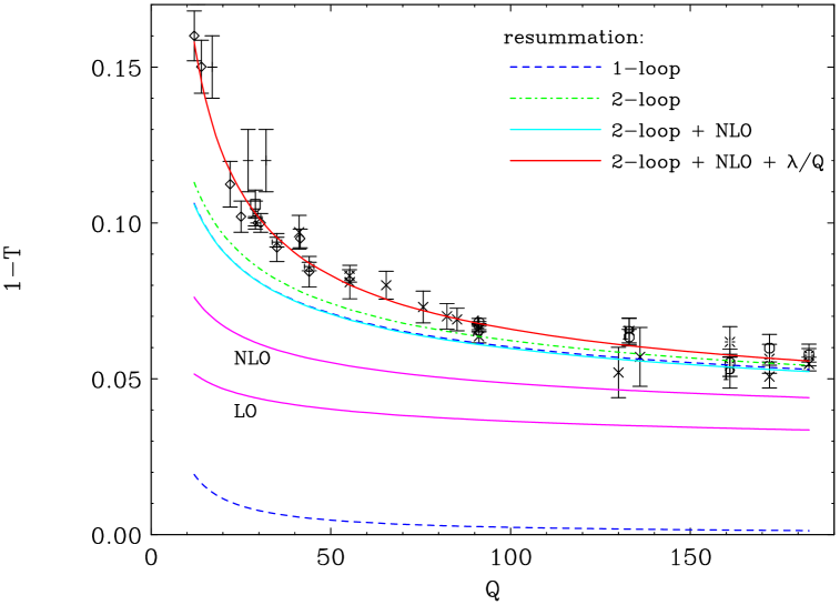
Figure 6: Average of $1-{\rm thrust}$: experimental data vs. naive and resummed QCD predictions, given $\alpha_{s}^{\hbox{$\overline{\hbox{\tiny MS}}\,$}}({\rm M_{Z}})=0.110$ – the value which yields the best fit in eq. (166). The resummation is performed with $\bar{a}_{\hbox{\tiny PT}}$ in the “gluon bremsstrahlung” scheme. See the caption of fig. 5 for further details.

While in fig. 6 the perturbative sum (165) by itself is not as close to the data, it is clear that the main conclusion we drew from fig. 5 concerning the significance of the resummation holds.

The curvature of $\chi^{2}$ as a function of $\alpha_{s}$ and $\lambda$ around the minimum reflects the spread of the experimental results. The two parameter fit of (166), calculated at two-loop, to the entire set of data points yields an experimental error of

$$\alpha_{s}^{\hbox{$\overline{\hbox{\tiny MS}}\,$}}({\rm M_{Z}})=0.110\pm 0.0017,$$ (167)

and

$$\lambda=0.62\pm 0.12\,{\rm GeV}$$ (168)

for a confidence level of $95\%$.

Further statistical analysis shows that the various experiments are quite consistent and that there is no significant difference between small $Q$ and large $Q$ data points as far as our fit is concerned. For instance, if we exclude the lowest data points $Q<22\,{\rm GeV}$, which seem quite spread, we find an improvement in the fit with a minimal $\chi^{2}/{\rm point}=1.15$ but the corresponding values of $\alpha_{s}$ and $\lambda$ change just a little, namely: $\alpha_{s}^{\hbox{$\overline{\hbox{\tiny MS}}\,$}}({\rm M_{Z}})=0.111$ and $\lambda=0.54\,{\rm GeV}$. If we exclude the highest data points $Q\geq 172\,{\rm GeV}$ we find $\chi^{2}/{\rm point}=1.44$ with the same central values as in (167) and (168). The most striking evidence that there is no systematic trend in the data which is missed by our fit is that even if we exclude all the data points above or below ${\rm M_{Z}}=91.2\,{\rm GeV}$, the best fit values are hardly affected: in the former case, having 29 data points, we get $\chi^{2}/{\rm point}=1.61$ with the same central values as in (167) and (168) and in the latter, having 20 data points, we get $\chi^{2}/{\rm point}=1.17$ with $\alpha_{s}^{\hbox{$\overline{\hbox{\tiny MS}}\,$}}({\rm M_{Z}})=0.111$ and $\lambda=0.53\,{\rm GeV}$. Note, however, that the effective experimental error changes significantly, e.g. in the latter case, the error in a two parameter fit with $95\%$ confidence level on the extracted value of $\alpha_{s}$ becomes $\pm 0.011$.

5.4 Truncation of the perturbative expansion

Let us consider now the expansion of the renormalon integral (18) in some renormalization scheme, e.g. the expansion (5.2) in $a_{\hbox{$\overline{\hbox{\tiny MS}}\,$}}(Q^{2})$. As explained in sec. 5.2 this series diverges at large orders due to the factorial increase of the coefficients induced by (infrared) renormalons. A standard procedure dealing with asymptotic expansions is to sum the series up to the minimal term. This can be regarded as an effective regularization of the all order sum.

As an example we analyze here the expansion (5.2) in some detail. Fig. 7 shows the increasing order partial sums at a given center of mass energy $Q={\rm M_{Z}}$ while fig. 8 shows the results obtained when truncating the series at the minimal term as a function of $Q$. In the latter, the relevant curve is made of four distinct pieces according to the number of terms included in the sum: the minimal term is reached between the sixth and the ninth term depending on $Q$. Both figures show that truncation at the minimal term is quite close to the principal value Borel sum regularization.

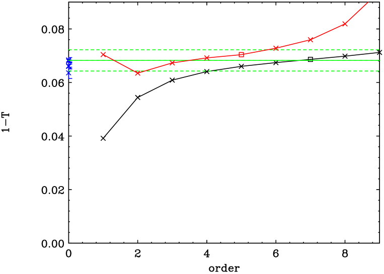
Figure 7: Partial sums corresponding to the expansion of the one-loop renormalon integral (18), with $\bar{a}_{\hbox{\tiny PT}}$ in the “gluon bremsstrahlung” scheme, in terms of $a_{\hbox{$\overline{\hbox{\tiny MS}}\,$}}(\mu_{R}^{2})$ as a function of the truncation order, for $Q={\rm M_{Z}}=91.2\,{\rm GeV}$ with $\alpha_{s}^{\hbox{$\overline{\hbox{\tiny MS}}\,$}}({\rm M_{Z}})=0.117$. The lower line corresponds to $\mu_{R}^{2}=Q^{2}$, eq. (5.2), and the upper line to $\mu_{R}^{2}=\mu_{\hbox{\tiny BLM}}^{2}$, eq. (5.4). The square symbol is the minimal term in each expansion. The horizontal band represents Borel summation, where the middle line is the principal value regularization and the two dashed lines show the estimated renormalon ambiguity based on the imaginary part of the Borel sum. The symbols on the left show the experimental data points. Note that the small next-to-leading order correction of (151) is not included in the theoretical results shown here.

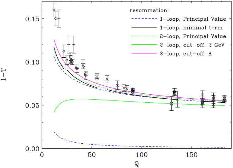
Figure 8: Comparison between different regularizations of the perturbative sum with $\bar{a}_{\hbox{\tiny PT}}$ in the “gluon bremsstrahlung” scheme for $\alpha_{s}^{\hbox{$\overline{\hbox{\tiny MS}}\,$}}({\rm M_{Z}})=0.110$ as a function of the center of mass energy $Q$. The regularizations shown are: one-loop (dashed) and two-loop (dot-dash) principal value Borel sum (or $R_{\hbox{\tiny APT}}$), truncation of the $\overline{\rm MS}$ expansion (5.2) at the minimal term and the two-loop $R_{\hbox{\tiny UV}}^{\hbox{\tiny PT}}$ with the cutoff scales $\mu_{I}=2\,{\rm GeV}$ and $\mu_{I}=\Lambda_{\hbox{\tiny brem}}^{\hbox{\tiny 2-loop}}=0.361\,{\rm GeV}$. Note that the small next-to-leading order correction of (151) is not included in the perturbative sum in this plot.

It is clear from fig. 7 that the contribution of the ${\cal O}(a_{\hbox{$\overline{\hbox{\tiny MS}}\,$}}^{3})$ and ${\cal O}(a_{\hbox{$\overline{\hbox{\tiny MS}}\,$}}^{4})$ terms is significant, as one could already guess based on the largeness of the ${\cal O}(a_{\hbox{$\overline{\hbox{\tiny MS}}\,$}}^{2})$ term in (135). The minimal term, which turns out to be close to the principal value Borel sum, is obtained for this center of mass energy at order ${\cal O}(a_{\hbox{$\overline{\hbox{\tiny MS}}\,$}}^{7})$. In (5.2), a new log-moment $f_{i}$ enters at each order in the perturbative expansion, such that the term ${\cal O}(a_{\hbox{$\overline{\hbox{\tiny MS}}\,$}}^{i})$ depends on all $f_{j}$ with $j<i$. From the definition of the log-moments (154) it follows that the larger the order $i$, the more sensitive $f_{i}$ is to the small $\epsilon$ behavior of ${\cal F}(\epsilon)$. Eventually, when the asymptotic regime is reached, the added terms reflect just the leading term in the small $\mu^{2}$ expansion of the characteristic function, namely the leading renormalon, which is related in our case to a $1/Q$ power correction. Since the value of the added non-perturbative term $\lambda/Q$ is determined by a fit, it may not be important at which order exactly the series is truncated, provided it is close enough to the asymptotic regime. On the other hand, a qualitative difference exists between truncation of the series at the minimal term and truncation much before the asymptotic regime, say at the next-to-leading order. The latter would not differ from a generic regularization of the perturbative sum just by power terms. This also implies that the value of $\alpha_{s}$ obtained by fitting the data with a next-to-leading order series plus a power term would be different than in the current approach.

Next consider, as a pedagogical exercise, a fit to experimental data based on the truncated expansion (5.2) in the $\overline{\rm MS}$ scheme, namely

$$\left<t\right> = \frac{C_{F}}{2}\left[\left.S_{0}^{\hbox{\tiny PT}}\right|_{{\cal O}(a^{k})}+\delta_{\hbox{\tiny NLO}}\right]\,+\,\frac{\lambda_{\rm pert}}{Q}$$

$$= \frac{C_{F}}{2}\left[t_{0}\,a_{\hbox{$\overline{\hbox{\tiny MS}}\,$}}(Q^{2})\,+\,t_{1}\,a_{\hbox{$\overline{\hbox{\tiny MS}}\,$}}^{2}(Q^{2})\,+\,\sum_{i=3}^{k}\,t_{i-1}^{0}\,a_{\hbox{$\overline{\hbox{\tiny MS}}\,$}}^{i}(Q^{2})\,\right]\,+\,\frac{\lambda_{\rm pert}}{Q}$$

where $k$ is the order of truncation. The fit results are listed in table 3 for $k=2$ through $6$. For these values of $k$ the series is still convergent: the diverging part of the expansion is not reached for any $Q$, since the minimal term is between the sixth and the ninth term. The coupling $a_{\hbox{$\overline{\hbox{\tiny MS}}\,$}}(Q^{2})$ in (5.4) is assumed to obey the two-loop renormalization group equation with $N_{f}=5$.

$$\begin{array}[]{|c|c|c|}\hline\cr\,k&\,\alpha_{s}^{\hbox{$\overline{\hbox{\tiny MS}}\,$}}({\rm M_{Z}})&\,\lambda_{\rm pert}\,({\rm GeV})\\ \hline\cr\hline\cr 2&0.128&0.72\\ \hline\cr 3&0.118&0.65\\ \hline\cr 4&0.115&0.58\\ \hline\cr 5&0.114&0.50\\ \hline\cr 6&0.114&0.40\\ \hline\cr\end{array}$$

Table 3: Fit results based on (5.4) using the expansion (5.2) up to order $k$.

Note that nothing can be learned from the quality of the fit: it is roughly the same in all cases, $\chi^{2}/{\rm point}\simeq 1.3$, and it is also very close to the resummation based fit of the previous section, $\chi^{2}/{\rm point}\simeq 1.33$. The corresponding experimental error in the extracted value of $\alpha_{s}$ in table 3 based on a two parameter fit with $95\%$ confidence level is $\pm 0.0024$.

Care should be taken comparing the results for $k=2$ in table 3 with the fit in [7] as well as with recent experimental fits [3]. In the latter, the finite infrared coupling formula of refs. [7, 8, 45] is used, namely the coefficient in front of the $1/Q$ term is modified, $\lambda\longrightarrow\lambda-\lambda_{\hbox{\tiny PT}}$ to avoid double counting in the perturbative and power correction pieces. Since $\lambda_{\hbox{\tiny PT}}$ depends on the coupling this change has an effect on the central values of the fit. For example, using the formula of [7, 8, 45] with the current data set one obtains at the next-to-leading order ($k=2$) a central value of $\alpha_{s}^{\hbox{$\overline{\hbox{\tiny MS}}\,$}}({\rm M_{Z}})=0.124$ (the Milan factor [45] is not included) rather than $\alpha_{s}^{\hbox{$\overline{\hbox{\tiny MS}}\,$}}({\rm M_{Z}})=0.128$.

Comparing table 3 with the resummation results of table 2 we find that the truncation leads to an overestimated value of $\alpha_{s}$. This comparison invalidates the next-to-leading order procedure of ref. [7, 8, 45]. As more terms are included, the value of $\alpha_{s}$ becomes closer to the resummation result, $\alpha_{s}^{\hbox{$\overline{\hbox{\tiny MS}}\,$}}({\rm M_{Z}})=0.111$. This value is not reached even for $k=6$: indeed there is a difference between a fixed order calculation and a regularized sum, e.g. in the principal value regularization. The latter is close, as we saw, to truncation of the series at the minimal term, but then the order of truncation is not fixed but rather depends on $Q$.

The most drastic change in table 3 is, of course, between the next-to-leading order based fit ($k=2$) and the $k=3$ fit which includes an estimated (153) next-to-next-to-leading order contribution from the “leading skeleton”, $t_{2}^{0}\,a_{\hbox{$\overline{\hbox{\tiny MS}}\,$}}^{3}$ with $t_{2}^{0}\simeq 188$. There is some uncertainty in the estimated coefficient $t_{2}^{0}$ so long as the identity of the “skeleton coupling” is not known. Here we assumed that $\bar{a}_{\hbox{\tiny PT}}$ is in the “gluon bremsstrahlung” scheme, and so we used $d_{1}=1-\frac{\pi^{2}}{4}$ in eq. (153). If we assume instead the pinch technique scheme, with $d_{1}=1$, we obtain $t_{2}^{0}\simeq 279$, which yields a best fit for $k=3$ at $\alpha_{s}^{\hbox{$\overline{\hbox{\tiny MS}}\,$}}({\rm M_{Z}})=0.114$ with $\lambda_{\rm pert}=0.66$ (cf. $k=3$ in table 3). Note that if $d_{1}$ (which characterizes the relation between the “skeleton scheme” and $\overline{\rm MS}$) is not large, it is the “large $\beta_{0}$” term (which is proportional to $\beta_{0}^{2}$ and independent of $d_{1}$) that dominates $t_{2}^{0}$ in eq. (153): $t_{2}^{0}\,=\,1.5776\,d_{1}^{2}\,+\,37.59\,d_{1}\,+\,239.62$.

We stress that the choice we made in (5.2) to expand $\overline{a}_{\hbox{\tiny eff}}^{\hbox{\tiny PT}}(\mu^{2})$ in terms of $a_{\hbox{$\overline{\hbox{\tiny MS}}\,$}}(Q^{2})$ is arbitrary. We could in principle pick any renormalization scale and scheme. A particularly good choice, using still the ${\overline{\rm MS}}$ scheme, is to set the scale equal to the BLM scale, namely to eliminate the term proportional to $\beta_{0}$ from the next-to-leading order coefficient

$$\mu^{2}_{\hbox{\tiny BLM}}=Q^{2}\exp\left(\frac{f_{1}}{f_{0}}+c_{1}\right)$$ (170)

yielding $\mu_{\hbox{\tiny BLM}}^{\hbox{$\overline{\hbox{\tiny MS}}\,$}}\simeq 0.0447\,Q$. We then obtain from (5.2) the following series

$$S_{0}^{\hbox{\tiny PT}}={f_{0}}\,a_{\hbox{$\overline{\hbox{\tiny MS}}\,$}}(\mu^{2}_{\hbox{\tiny BLM}}) + {d_{1}}\,{f_{0}}\,a_{\hbox{$\overline{\hbox{\tiny MS}}\,$}}^{2}(\mu^{2}_{\hbox{\tiny BLM}})$$

$$+ \left\{{d_{1}}^{2}\,{f_{0}}-{\frac{1}{3}}\,{\frac{3\,{f_{1}}^{2}+\pi^{2}\,{f_{0}}^{2}-3\,{f_{2}}\,{f_{0}}}{{f_{0}}}}\,\beta_{0}^{2}\right\}\,a_{\hbox{$\overline{\hbox{\tiny MS}}\,$}}^{3}(\mu^{2}_{\hbox{\tiny BLM}})+\cdots$$

which provides a good approximation to $R_{\hbox{\tiny APT}}\simeq R_{\hbox{\tiny PT}|\hbox{\tiny PV}}$ already at the leading order, as shown in fig. 7. We mention that a particularly low renormalization scale was suggested for this observable in [12, 13]. Such a choice can now be justified from another view point, noting that the BLM scale approximates well the resummed perturbative series.

The proximity of the leading order BLM result to the Borel sum in fig. 7 suggests that performing the fit based on a next-to-leading order partial sum in $\overline{\rm MS}$ with $\mu_{R}=\mu_{\hbox{\tiny BLM}}$ would be much better than with $\mu_{R}=Q$ corresponding to $k=2$ in table 3. Indeed, performing such a fit (with a power term of the form $\lambda_{\rm pert}/Q$), we find a significant change in the extracted parameters. The central value is $\alpha_{s}^{\hbox{$\overline{\hbox{\tiny MS}}\,$}}({\rm M_{Z}})=0.116$ (with $\lambda_{\rm pert}=0.55\,{\rm GeV}$), which is much closer to the best fit result of our resummation, $\alpha_{s}^{\hbox{$\overline{\hbox{\tiny MS}}\,$}}({\rm M_{Z}})=0.111$. It should be noted that the results do not coincide: leading order BLM scale-setting is not a substitute to actually performing the resummation (see related observations in [25]).

Note that the success of BLM in ${\overline{\rm MS}}$ is not guaranteed a priori. It is the smallness of $d_{1}$ in the relation (7) between the scheme coupling (chosen as ${\overline{\rm MS}}$) and the “skeleton coupling” (assumed to be the “gluon bremsstrahlung”coupling) which plays a role here. The most natural scheme to apply BLM is the “skeleton scheme” $\bar{a}_{\hbox{\tiny PT}}$, where $c_{1}=d_{1}=0$. Then, similarly to the Euclidean case (15), there is a scheme invariant interpretation to the BLM scale

$$\mu^{2}_{\hbox{\tiny BLM}}=Q^{2}\exp\left(\frac{f_{1}}{f_{0}}\right)$$ (172)

as the center of $\dot{\cal F}(\epsilon)$. In the case of the average thrust it is

$$\mu_{\hbox{\tiny BLM}}=0.1028\,Q,$$ (173)

as can be verified directly in fig. 4. Now the leading term in the BLM expansion (5.4) is $f_{0}\,\bar{a}_{\hbox{\tiny PT}}(\mu_{\hbox{\tiny BLM}}^{2})$ and the next-to-leading order correction vanishes. Higher order corrections have a simple interpretation [26, 29] in terms of the properties for the function $\dot{\cal F}(\epsilon)$. For instance, the next-to-next-to-leading order is related to the width of $\dot{\cal F}(\epsilon)$ through its second moment $f_{2}$.

5.5 Cutoff regularization and the infrared finite coupling approach

As explained in sec. 3.3 the cutoff regularized perturbative sum $R_{\hbox{\tiny UV}}^{\hbox{\tiny PT}}$ of eq. (55) is of special interest because it is fully under control in perturbation theory. In particular, in this regularization the replacement of the all order coupling $\bar{a}_{\hbox{\tiny PT}}$ by a one-loop or two-loop coupling is justified provided $\mu_{I}/\Lambda$ is large enough. In addition, as we saw in sec. 4, the infrared cutoff regularization appears naturally in the framework of the infrared finite coupling [7, 8]. Let us therefore repeat the analysis of the average thrust in terms of this regularization.

In general, $R_{\hbox{\tiny UV}}^{\hbox{\tiny PT}}$ can be obtained from $R_{\hbox{\tiny APT}}$ by $R_{\hbox{\tiny UV}}^{\hbox{\tiny PT}}=R_{\hbox{\tiny APT}}-\Delta R$. Since in our case ${\rm Re}\left\{\delta R_{\hbox{\tiny APT}}\right\}$ is negligibly small, we simply have $\Delta R\simeq{\rm Re}\left\{R^{\hbox{\tiny PT}}_{\hbox{\tiny IR}}\right\}$. The ${\cal O}(1/Q^{2n})$ contribution corresponding to the $n$-th order term in (5.1) is given by eq. (3.3) and eq. (114) with (101) (or equivalently eq. (118)) in the one and two loop cases, respectively. The leading $n=\frac{1}{2}$ term is given in the one-loop case by

$$\left.{\rm Re}\left\{R^{\hbox{\tiny PT}}_{\hbox{\tiny IR},\frac{1}{2}}\right\}\right|_{\hbox{\tiny 1-loop}}=\left(\frac{\mu_{I}}{Q}\right)\frac{-C_{T}^{\left(\frac{1}{2}\right)}}{\beta_{0}\pi}\,e^{-\frac{t_{I}}{2}}\,{\rm Ei}\left(\frac{t_{I}}{2}\right)$$ (174)

with $t_{I}\equiv\ln\left(\mu_{I}^{2}/\Lambda^{2}\right)$ and in the two-loop case by

$$\left.{\rm Re}\left\{R^{\hbox{\tiny PT}}_{\hbox{\tiny IR},\frac{1}{2}}\right\}\right|_{\hbox{\tiny 2-loop}}=\left(\frac{\mu_{I}}{Q}\right)\frac{-C_{T}^{\left(\frac{1}{2}\right)}}{\beta_{0}\pi}\,e^{-\frac{\tilde{t}_{I}}{2}}\,{\rm Re}\left\{-\left(-\frac{\tilde{t}_{I}}{2}\right)^{\delta}\,\Gamma\left(-\delta,-\frac{\tilde{t}_{I}}{2}\right)\right\}$$ (175)

with $\tilde{t}_{I}\equiv 1/(\beta_{0}\tilde{a}_{I})$ where $\tilde{a}_{I}$ is defined in (100) and $\delta=\delta_{\frac{1}{2}}=\frac{1}{2}\left(\beta_{1}/\beta_{0}^{2}\right)$ according to eq. (99).

Choosing $\mu_{I}=2\,{\rm GeV}$, with the same value of $\alpha_{s}$ as in fig. 5, we obtain the cutoff regularized sum $\left<t\right>_{\hbox{\tiny PT}}=\frac{Cf}{2}R_{\hbox{\tiny UV}}^{\hbox{\tiny PT}}$ which is presented in fig. 9.

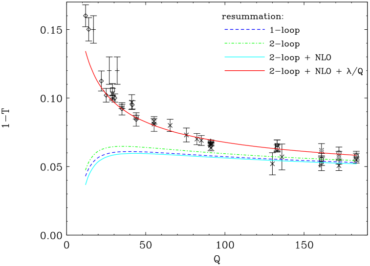
Figure 9: Cutoff regularized perturbative sum with $\mu_{I}=2\,{\rm GeV}$, given $\alpha_{s}^{\hbox{$\overline{\hbox{\tiny MS}}\,$}}({\rm M_{Z}})=0.117$. As in fig. 5, the resummation is calculated with $\bar{a}_{\hbox{\tiny PT}}$ as a one or two loop coupling in the “gluon bremsstrahlung” scheme. In the two-loop case we show also a curve that includes the full ${\cal O}(\alpha_{s}^{2})$ term, as well as a best fit curve that includes in addition a fitted $\lambda/Q$ correction (176).

Comparing fig. 9 with fig. 5, the first observation is that $R_{\hbox{\tiny UV}}^{\hbox{\tiny PT}}(Q^{2})$ is significantly lower than $R_{\hbox{\tiny APT}}(Q^{2})$ (or $R_{\hbox{\tiny PT}|\hbox{\tiny PV}}(Q^{2})$), especially for low $Q$. This means that a major contribution to the resummation (18) is from space-like momentum scales below the cutoff $\mu_{I}=2\,{\rm GeV}$, i.e. from large distance scales in which the perturbative treatment does not apply. This point will be elaborated in the conclusion section.

As discussed in sec. 3.3, the replacement of the all order coupling by some approximation like the one or two loop coupling is best justified in terms of the cutoff regularization. It is thus important to verify that $R^{\hbox{\tiny PT}}_{\hbox{\tiny UV}}$ remains stable going from one to two loops. Fig. 9 shows that indeed even at low $Q$ the difference between the one and two loop $R_{\hbox{\tiny UV}}^{\hbox{\tiny PT}}(Q^{2})$ is rather small. We conclude that $R_{\hbox{\tiny UV}}^{\hbox{\tiny PT}}(Q^{2})$ is under perturbative control for $\mu_{I}=2\,{\rm GeV}$. To improve further the accuracy at which $R_{\hbox{\tiny UV}}^{\hbox{\tiny PT}}(Q^{2})$ is determined one can, in principle, either go to higher orders in the $\beta$ function of $\bar{a}_{\hbox{\tiny PT}}$ or increase $\mu_{I}$. In the latter case, however, one should be careful not to invalidate the expansion of $\dot{\cal F}(\mu^{2}/Q^{2})$ in $\Delta R$ (or $\Phi(k^{2}/Q^{2})$ in $R^{\hbox{\tiny PT}}_{\hbox{\tiny IR}}$) which holds only for small enough $\mu_{I}^{2}/Q^{2}$. The physical value of $\mu_{I}$, separating at once short distance physics from large distance physics and the perturbative domain from the non-perturbative one, should be set satisfying these two constraints.

Next, we fit the data with

$$\left<t\right>=\frac{C_{F}}{2}\left[R_{\hbox{\tiny UV}}^{\hbox{\tiny PT}}+\delta_{\hbox{\tiny NLO}}\right]+\frac{\lambda_{\mu_{I}}}{Q}.$$ (176)

The best fit values of $\lambda_{2\,{\rm GeV}}$ for $a_{\hbox{$\overline{\hbox{\tiny MS}}\,$}}({\rm M_{Z}})=0.117$ (fig. 9) are listed in table 4 below. Note that the fit (176) in fig. 9, and the fit (166) in fig. 5 are almost identical. This is reflected also in the similar $\chi^{2}$ values quoted in tables 4 and 1. The reason is that the two regularizations, $R_{\hbox{\tiny APT}}$ (or $R_{\hbox{\tiny PT}|\hbox{\tiny PV}}$) and $R_{\hbox{\tiny UV}}^{\hbox{\tiny PT}}(Q^{2})$ differ, to a very good approximation, just by the $1/Q$ power correction of the type we add as a free parameter in the fit (see sec. 4). One can thus check that the difference between the fitted parameters in the two regularizations is as implied by the calculation. For instance, in the one-loop case, the difference is calculable from eq. (174), namely

$$\lambda_{\mu_{I}}-\lambda\simeq\mu_{I}\,\frac{C_{F}}{2}\,\frac{-C_{T}^{\left(\frac{1}{2}\right)}}{\beta_{0}\pi}e^{-\frac{t_{I}}{2}}{\rm Ei}\left(\frac{t_{I}}{2}\right).$$ (177)

$$\begin{array}[]{|c|c|c|}\hline\cr\,\bar{a}_{\hbox{\tiny eff}}^{\hbox{\tiny PT}}&\,\lambda_{2\,{\rm GeV}}\,({\rm GeV})&\,\chi^{2}/{\rm point}\\ \hline\cr\hline\cr{\rm one-loop}&1.32&2.43\\ \hline\cr{\rm two-loop}&1.14&3.46\\ \hline\cr\end{array}$$

Table 4: Power term ($\lambda_{2\,{\rm GeV}}$) fit results with $\alpha_{s}^{\hbox{$\overline{\hbox{\tiny MS}}\,$}}({\rm M_{z}})=0.117$ based on (176).

The sub-leading power term making $R_{\hbox{\tiny PT}|\hbox{\tiny PV}}$ and $R_{\hbox{\tiny UV}}^{\hbox{\tiny PT}}$ different is related to the next non-analytic term in the expansion of ${\cal F}(\epsilon)$, $n=\frac{3}{2}$, which leads to negligibly small $1/Q^{3}$ power corrections. As mentioned above, the latter are calculable using eq. (3.3) and (118) in the one and two loop cases, respectively.

The effect of leading and sub-leading power terms in the expansion of ${\cal F}(\epsilon)$ in (5.1) is summarized in table 5 for the lowest experimentally relevant energy $Q=12\,{\rm GeV}$.

$$\begin{array}[]{|c||c|c||c||c|c|}\hline\cr&&&&&\\ \,n^{\,}&{{C_{F}}\over{2}}{\rm Re}\left\{R_{\hbox{\tiny IR}}^{\hbox{\tiny PT}}\right\}&\frac{C_{F}}{2}{\rm Re}\left\{\delta R_{\hbox{\tiny APT}}\right\}&\frac{C_{F}}{2}\Delta R&\frac{C_{F}}{2}\left(R_{\hbox{\tiny IR}}^{\hbox{\tiny PT}}-R_{<}^{\hbox{\tiny PT}}\right)&\frac{C_{F}}{2}R_{<}^{\hbox{\tiny APT}}\\ \hline\cr\,\frac{1}{2}_{\,}&0.0796&0&0.0796&-0.0401&0.1197\\ \hline\cr\,1_{\,}&0&\,0.701\,\,10^{-3}&0.701\,\,10^{-3}&0.0341&-0.0334\\ \hline\cr\,\frac{3}{2}_{\,}&-0.131\,\,10^{-2}&0&-0.131\,\,10^{-2}&-0.666\,\,10^{-2}&\,0.535\,\,10^{-2}\\ \hline\cr\,2_{\,}&-0.822\,\,10^{-4}&\,0.663\,\,10^{-7}&-0.821\,\,10^{-4}&\,0.353\,\,10^{-4}&-0.117\,\,10^{-3}\\ \hline\cr\end{array}$$

Table 5: Contributions ${\cal O}(1/Q^{2n})$ from increasing order terms in the expansion of ${\cal F}(\epsilon)$ to the difference between different regularizations of the perturbative sum with the one-loop running coupling in the “gluon bremsstrahlung” scheme, at $Q=12\,{\rm GeV}$. The infrared cutoff is set to $\mu_{I}=2\,{\rm GeV}$. For comparison, at this energy $\left<t\right>\simeq\frac{C_{F}}{2}R_{\hbox{\tiny APT}}=0.1233$.

Table 5 contains contributions of both analytic and non-analytic terms in ${\cal F}(\epsilon)$. It presents the two possible separations of $\Delta R$ discussed in sec. 3.3 – the separation into ${\rm Re}\left\{R_{\hbox{\tiny IR}}^{\hbox{\tiny PT}}\right\}$ and ${\rm Re}\left\{\delta R_{\hbox{\tiny APT}}\right\}$, corresponding to eq. (85), on the left side of the table, and the separation into $R_{\hbox{\tiny IR}}^{\hbox{\tiny PT}}-R_{<}^{\hbox{\tiny PT}}$ and $R_{<}^{\hbox{\tiny APT}}$, corresponding to eq. (83) on the right. We find that in the separate pieces on the right the sub-leading terms (e.g. $n=1$) are relatively important, while not so on the left, where the total $\Delta R$ can be approximated by the leading ${\rm Re}\left\{R_{\hbox{\tiny IR}}^{\hbox{\tiny PT}}\right\}$ piece

$$\Delta R\simeq{\rm Re}\left\{R_{\hbox{\tiny IR},\frac{1}{2}}^{\hbox{\tiny PT}}\right\}.$$ (178)

Next, consider the dependence of the cutoff regulated perturbative sum $R^{\hbox{\tiny PT}}_{\hbox{\tiny UV}}(Q^{2})$ on the cutoff scale $\mu_{I}$. Any two cutoff regularizations differ, in general, by renormalon related infrared power corrections. In our case, they differ to a very good approximation by a $1/Q$ term which can be calculated using eq. (174) and (175) in the one and two loop cases, respectively. As a result, one would practically obtain the same best fit in (176) for any arbitrary $\Lambda\leq\mu_{I}\ll Q$. In the two-loop case, $R^{\hbox{\tiny PT}}_{\hbox{\tiny UV}}(Q^{2})$ is well defined even for the extreme choice $\mu_{I}=\Lambda$. The resulting regularization is shown in fig. 8 together with the standard $\mu_{I}=2\,{\rm GeV}$ choice. The $\mu_{I}=\Lambda$ regularization turns out to be close to the best fit in this case. This regularization is, of course, unacceptable in the infrared finite coupling approach [7, 8], where one requires that the non-perturbative coupling $\bar{a}$ is well approximated by $\bar{a}_{\hbox{\tiny PT}}$ above $\mu_{I}$. As explained in sec. 4, within the infrared finite coupling approach, the non-perturbative parameter $\lambda_{\mu_{I}}$ acquires a physical interpretation as the small gluon virtuality moment of the “skeleton coupling”. Using (133) with (5.1), we have

$$R_{\hbox{\tiny IR}}=\int_{0}^{\mu_{I}^{2}}\bar{a}(k^{2})\,\Phi\left(k^{2}/Q^{2}\right)\,\frac{dk^{2}}{k^{2}}\simeq-\left(\frac{\mu_{I}}{Q}\right)C_{T}^{\left(\frac{1}{2}\right)}\,\frac{2}{\pi}\,\frac{1}{\mu_{I}}\int_{0}^{\mu_{I}}\bar{a}(k)dk$$ (179)

which implies

$$\lambda_{\mu_{I}}=-\mu_{I}\frac{C_{F}}{2}C_{T}^{\left(\frac{1}{2}\right)}\,\frac{2}{\pi}\,\frac{1}{\mu_{I}}\int_{0}^{\mu_{I}}\bar{a}(k)dk.$$ (180)

We stress that the identification of the fit parameter $\lambda_{\mu_{I}}$ with a small virtuality moment of the coupling is meaningful only under the strong assumption of universality: it is the same “skeleton coupling” for any observable. Eq. (180) as written implies that the coefficient in front of the “skeleton coupling” average is simply related to the small $\mu^{2}$ behavior of the characteristic function, in spite of the non-inclusive nature of the thrust. In ref. [45] it is argued that this coefficient is in fact modified by the so called “Milan factor” arising at the next-to-leading order level, taking into account the emission of two gluons. We ignore these corrections here (see sec. 5.6).

Let us now extract $\lambda_{2\,{\rm GeV}}$ based on the best fit of (176). As we know already from sec. 5.3 (see table 2), the best fit is obtained in the one-loop case at $\alpha_{s}^{\hbox{$\overline{\hbox{\tiny MS}}\,$}}({\rm M_{Z}})=0.111$. The corresponding power correction coefficient in the cutoff regularization is $\lambda_{2\,{\rm GeV}}=1.57\pm 0.12\,{\rm GeV}$, where the error corresponds to the combined systematic and statistical experimental uncertainties. In the two-loop case, the best fit is at $\alpha_{s}^{\hbox{$\overline{\hbox{\tiny MS}}\,$}}({\rm M_{Z}})=0.110$ with $\lambda_{2\,{\rm GeV}}=1.49\pm 0.12\,{\rm GeV}$. In the latter case the cutoff regularized sum and the best fit are shown in fig. 10.

According to eq. (180) we have for $\mu_{I}=2\,{\rm GeV}$

$$\frac{1}{\mu_{I}}\int_{0}^{\mu_{I}}\bar{a}(k)dk=-\frac{\lambda_{\mu_{I}}}{\mu_{I}}\frac{\pi}{C_{F}}\frac{1}{C_{T}^{\left(\frac{1}{2}\right)}}=\left\{\begin{array}[]{ll}0.231\pm 0.017&\,\,\,\,\,\,\,\,\,\,\,{\rm one-loop}\\ 0.219\pm 0.017&\,\,\,\,\,\,\,\,\,\,\,{\rm two-loop}\\ \end{array}\right.$$ (181)

where $\bar{a}$ is the “gluon bremsstrahlung” coupling.

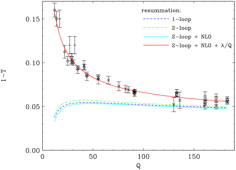
Figure 10: Cutoff regularized perturbative sum with $\mu_{I}=2\,{\rm GeV}$, for the best fit value $\alpha_{s}^{\hbox{$\overline{\hbox{\tiny MS}}\,$}}({\rm M_{Z}})=0.110$. As in fig. 6, the resummation is calculated with $\bar{a}_{\hbox{\tiny PT}}$ as a one or two loop coupling in the “gluon bremsstrahlung” scheme. In the two-loop case we show also a curve that includes the full ${\cal O}(\alpha_{s}^{2})$ term, as well as a best fit curve that includes in addition a fitted $\lambda/Q$ correction (176).

5.6 Sources of theoretical uncertainty

The experimental error on the value of $\alpha_{s}$ and $\lambda$ was discussed in sec. 5.3. The theoretical error, which is harder to determine, will be briefly discussed here.

A primary source of uncertainty is the unknown identity of the running coupling used in the calculation of $R_{\hbox{\tiny APT}}$. In sec. 5.3 we approximated this coupling by the one or two loop coupling in the “gluon bremsstrahlung” scheme with $\beta_{0}$ and $\beta_{1}$ calculated for $N_{f}=5$. In principle, this coupling should be an “all-order” coupling in the “skeleton scheme” (yet unknown), where the number of active flavors depends on the scale. Let us try to quantify the errors.

Five active flavors: Considering the center of mass energy of most relevant experiments, using the running coupling with $N_{f}=5$ is known to be a reasonable approximation in the standard perturbative approach. However, in the resummation performed here the coupling runs over small gluon virtualities as well, and then there are only four or three active flavors. The significance of the $N_{f}=5$ approximation in our approach can be checked by calculating the difference between the contribution to perturbative sum $R_{\hbox{\tiny APT}}$ from small space-like momentum scales with $N_{f}=3$ or $4$ and the corresponding contribution with $N_{f}=5$. We use for this calculation the formula for $R_{\hbox{\tiny IR},\frac{1}{2}}^{\hbox{\tiny APT}}$ at the one-loop order, which is obtained in the Appendix, eq. (187) and (188). The relative difference between $R_{\hbox{\tiny IR},\frac{1}{2}}^{\hbox{\tiny APT}}(N_{f}=3)$ and $R_{\hbox{\tiny IR},\frac{1}{2}}^{\hbox{\tiny APT}}(N_{f}=5)$ for the lowest experimental data point $Q=12\,{\rm GeV}$, where the effect is the largest, is just $1.9$ percent. This is negligible compared to other sources of error.

Two-loop coupling: In the phenomenological analysis we used the one or two loop coupling to evaluate the perturbative sum, instead of the “all order skeleton coupling”. As explained in sec. 3.3 this replacement is justified in the cutoff regularization provided $\mu_{I}/\Lambda$ is large enough. Indeed we saw in sec. 5.5 (see figs. 9 and 10) that the cutoff regularized sum $R^{\hbox{\tiny PT}}_{\hbox{\tiny UV}}$ with $\mu_{I}=2\,{\rm GeV}$ does not change much going from one to two loops. This stability suggests that the replacement of the all order coupling by some low order coupling is a reasonable approximation for this value of the cutoff. To go further one would like to examine the effect of a three-loop correction $\beta_{2}$ in the $\beta$ function of the “skeleton coupling” on $R^{\hbox{\tiny PT}}_{\hbox{\tiny UV}}$. However, technically, this is a complicated task. Below, we shall examine instead the effect on $R_{\hbox{\tiny APT}}$. At the one and two loop level $R_{\hbox{\tiny APT}}$ is rather stable, as shown in figs. 5 and 6. A priori, the stability of $R_{\hbox{\tiny APT}}$ or the principal value Borel sum may be less intuitive because these regularizations do involve the coupling in the infrared. The stability of $R_{\hbox{\tiny APT}}$ may be explained in terms of the infrared stability of the APT coupling itself, which is discussed in [32, 40, 38], and goes beyond the two-loop level. Returning to our case, the effect of a three-loop correction in $\beta(\bar{a})$ on $R_{\hbox{\tiny APT}}$ can be examined explicitly. Since we do not know the identity of the “skeleton coupling”, we just try various choices of $\beta_{2}$ where for simplicity we use the Padé improved form of the three-loop $\beta$ function which can be solved analytically using the Lambert W function [38]. As an example consider the case where the $\beta$ function is modified to include a large three-loop term, $\beta_{2}/\beta_{0}=-45$ (both positive and negative values were studied). Taking the world average value of $\alpha_{s}$ ($\alpha_{s}^{\hbox{$\overline{\hbox{\tiny MS}}\,$}}({\rm M}_{Z})=0.117$) we obtain at the lowest experimental data point $Q=12\,{\rm GeV}$, where the effect is the largest, the following results for $\left<t\right>\simeq\frac{C_{F}}{2}R_{\hbox{\tiny APT}}$: at one-loop $\left<t\right>\simeq 0.123$, at two-loop $\left<t\right>\simeq 0.131$, and at three-loop $\left<t\right>\simeq 0.116$. These differences are small compared to the experimental error bars. The conclusion remains the same: the perturbative sum is quite stable with respect to including higher orders in the $\beta$ function. Whichever regularization is chosen, what counts at the end is to what extent the extracted parameters depend on the approximation used for the perturbative coupling. It is clear from table 2 that the resummation procedure is quite stable going from one to two loops concerning the determination of $\alpha_{s}$. In particular, the resulting uncertainty in the extracted value of $\alpha_{s}$ is smaller than the experimental error (167). Moreover, as we saw, one can use either $R_{\hbox{\tiny APT}}$ or $R^{\hbox{\tiny PT}}_{\hbox{\tiny UV}}$ obtaining the same value of $\alpha_{s}$. Thus, based on the stability of $R_{\hbox{\tiny APT}}$ at three-loop we conclude that the extracted value of $\alpha_{s}$ will remain stable, despite our lack of knowledge concerning the stability of $R^{\hbox{\tiny PT}}_{\hbox{\tiny UV}}$ at this level. On the other hand, for the determination of the power correction or the low momentum average of the coupling, the relevant theoretical uncertainty is comparable to the experimental error. This is reflected for example in the difference between the one and two loop results in tables 1 and 4. Similarly we have for $\alpha_{s}=0.110$,

$$\begin{array}[]{|c|c|c|}\hline\cr&{\rm APT\,/\,PV}&{\rm cutoff}\\ \,\bar{a}_{\hbox{\tiny eff}}^{\hbox{\tiny PT}}&\,\,\,\,\,\,\lambda\,({\rm GeV})&\,\lambda_{2\,{\rm GeV}}\,({\rm GeV})\\ \hline\cr\hline\cr{\rm one-loop}&0.79&1.62\\ \hline\cr{\rm two-loop}&0.62&1.49\\ \hline\cr\end{array}$$

Table 6: Power term fit results with $\alpha_{s}^{\hbox{$\overline{\hbox{\tiny MS}}\,$}}({\rm M_{z}})=0.110$.

Here it is important, in principle, which regularization is used. In our case, as shown in table 6, the cutoff regularization with $\mu_{I}=2\,{\rm GeV}$ yields slightly more stable values of the power correction coefficient than the principal value Borel sum (or APT) regularization. Nevertheless, this uncertainty in $\lambda_{\mu_{I}}$ is significant and should be taken into account when discussing the universality of the infrared finite coupling.

“gluon bremsstrahlung” scheme: In the phenomenological analysis above we used the “gluon bremsstrahlung” renormalization scheme as the scheme of the “skeleton coupling” $\bar{a}_{\hbox{\tiny PT}}$. As explained in sec. 2, the “skeleton coupling” should actually be defined diagrammatically in a unique way and the only thing we know about it, is that it coincides with the V-scheme in the Abelian limit. Alternative schemes were discussed in sec. 2 and 5.2. Of particular interest is the pinch technique coupling which has some systematic justification [22] and which differs from the “gluon bremsstrahlung” scheme by having a relatively large next-to-leading order correction (160) on top of the terms included in the resummation. The leading ${\cal O}(a^{2})$ “scheme dependence” effects corresponding to taking $\bar{a}_{\hbox{\tiny PT}}$ in different schemes cancel between $R_{\hbox{\tiny APT}}$ and remaining next-to-leading order correction in eq. (165). The residual dependence is thus formally of order $a^{3}$. In order to check the sensitivity of our procedure to the choice of $\bar{a}_{\hbox{\tiny PT}}$, we repeated the whole analysis with $\bar{a}_{\hbox{\tiny PT}}$ as $a_{\hbox{\tiny pinch}}$. Starting as in sec. 5.3 with the world average value of $\alpha_{s}$, $\alpha_{s}^{\hbox{$\overline{\hbox{\tiny MS}}\,$}}({\rm M_{Z}})=0.117$ which corresponds to $\Lambda_{\hbox{\tiny pinch}}^{\hbox{\tiny 1-loop}}=0.274\,{\rm GeV}$ and $\Lambda_{\hbox{\tiny pinch}}^{\hbox{\tiny 2-loop}}=0.686\,{\rm GeV}$, we obtain the results shown in fig. 11.

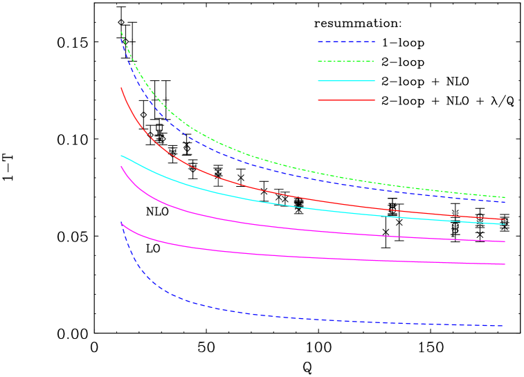
Figure 11: Principal value Borel sum (or $R_{\hbox{\tiny APT}}$) regularization of the perturbative sum (18) with the “skeleton coupling” $\bar{a}_{\hbox{\tiny PT}}$ in the pinch technique scheme [22], given $\alpha_{s}^{\hbox{$\overline{\hbox{\tiny MS}}\,$}}({\rm M_{Z}})=0.117$. For more details, see the caption in fig. 5.

Here the resummation result, namely $R_{\hbox{\tiny APT}}$ or principal value Borel sum with $\bar{a}_{\hbox{\tiny PT}}$ at one-loop or two-loops, overshoots most data points and especially the large $Q$ ones. However, after including the next-to-leading order correction (165) with the appropriate negative coefficient (160), the perturbative result becomes again quite close to the large $Q$ data points. Adding a power correction (166) the best fit (with $\bar{a}_{\hbox{\tiny PT}}$ at two-loop) is obtained for $\lambda=0.44\,{\rm GeV}$, with $\chi^{2}/{\rm point}=4.35$. In the infrared cutoff regularization with $\mu_{I}=2\,{\rm GeV}$ the same fit is obtained with $\lambda_{2\,{\rm GeV}}=1.53\,{\rm GeV}$. Finally, we fit also $\alpha_{s}$ using $\bar{a}_{\hbox{\tiny PT}}$ in the pinch scheme. The results of the best fit are shown in fig. 12.

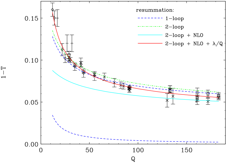
Figure 12: Principal value Borel sum (or $R_{\hbox{\tiny APT}}$) regularization of the perturbative sum (18) with the “skeleton coupling” $\bar{a}_{\hbox{\tiny PT}}$ in the pinch technique scheme [22], for the best fit value of $\alpha_{s}^{\hbox{$\overline{\hbox{\tiny MS}}\,$}}({\rm M_{Z}})=0.109$. For more details, see the caption in fig. 5.

The best fit with the two-loop running coupling in this scheme is obtained for $\alpha_{s}^{\hbox{$\overline{\hbox{\tiny MS}}\,$}}({\rm M_{Z}})=0.109$, with a power correction $\lambda=0.83\,{\rm GeV}$ in the principal value regularization and $\lambda_{2\,{\rm GeV}}=1.85\,{\rm GeV}$ in the cutoff regularization. In this fit $\chi^{2}/{\rm point}=1.37$. The comparison of these results with eqs. (167) and (168) suggests that precise identification of the “skeleton coupling” $\bar{a}_{\hbox{\tiny PT}}$ is not crucial in this case for the determination of $\alpha_{s}$.

Another possible source of uncertainty are ${\cal O}(a^{3})$ terms which are not related to the “leading skeleton”. At the single dressed gluon approximation level, such effects can be taken into account by calculating

$$\left<t\right>_{\hbox{\tiny PT}}(Q^{2})\,\simeq\,\frac{C_{F}}{2}\,\left[S_{0}^{\hbox{\tiny PT}}(Q^{2})\,+\,\tilde{t}_{1}\,a^{2}\,+\,\tilde{t}_{2}\,a^{3}\right]$$ (182)

instead of (150) where only the next-to-leading term was included. The coefficient $\tilde{t}_{2}$ can be determined from the full next-to-next-to-leading order perturbative coefficient $t_{2}$, $\tilde{t}_{2}=t_{2}-t_{2}^{0}$, once the time-like “skeleton coupling” $\bar{a}_{\hbox{\tiny eff}}^{\hbox{\tiny PT}}$ in (18) and the scheme coupling $a$ are specified. Unfortunately, $t_{2}$ is not known yet. Since the running coupling effects we resum here are understood to be the major source of growth of the standard coefficients $t_{i}$, the general expectation is that the remaining coefficients $\tilde{t}_{i}$ are small. Nevertheless, let us see what are the consequences if this assumption does not hold. We proceed as before using the coupling $a=R_{\hbox{\tiny APT}}(Q^{2})/f_{0}$

$$\left<t\right>_{\hbox{\tiny PT}}(Q^{2})\,\simeq\,\frac{C_{F}}{2}\,R_{\hbox{\tiny APT}}\left[1\,+\,\frac{\tilde{t}_{1}}{f_{0}}\,a\,+\,\frac{\tilde{t}_{2}}{f_{0}}\,a^{2}\right].$$ (183)

For the perturbative expansion to make sense one should require that the next-to-next-to-leading order term would be smaller than the leading term, i.e. $\tilde{t}_{2}/f_{0}<1/a^{2}$ or $\tilde{t}_{2}/f_{0}<f_{0}^{2}/R_{\hbox{\tiny APT}}^{2}$. For the lowest data points $Q=12\,{\rm GeV}$ the r.h.s. equals roughly $64$ so we shall consider possible next-to-next-to-leading corrections with $\left|\tilde{t}_{2}/f_{0}\right|\mathrel{\mathchoice{\vbox{\offinterlineskip\halign{$\m@th\displaystyle\hfil#\hfil$\cr<\crcr\sim\crcr} }}{\vbox{\offinterlineskip\halign{$\m@th\textstyle\hfil#\hfil$\cr<\crcr\sim\crcr} }}{\vbox{\offinterlineskip\halign{$\m@th\scriptstyle\hfil#\hfil$\cr<\crcr\sim\crcr} }}{\vbox{\offinterlineskip\halign{$\m@th\scriptscriptstyle\hfil#\hfil$\cr<\crcr\sim\crcr} }}}64$. Once $\tilde{t}_{2}$ is fixed we can fit the thrust data with (183) plus a $\lambda/Q$ power term. The results of such a fit turn out to depend significantly on the value of $\tilde{t}_{2}$. For instance, with $\tilde{t}_{2}/f_{0}=-63$, the best fit is obtained for $\alpha_{s}^{\hbox{$\overline{\hbox{\tiny MS}}\,$}}({\rm M_{Z}})=0.117$ with $\lambda=2.4\,{\rm GeV}$ and $\chi^{2}/{\rm point}=1.478$ while for $\tilde{t}_{2}/f_{0}=56$ the best fit is $\alpha_{s}^{\hbox{$\overline{\hbox{\tiny MS}}\,$}}({\rm M_{Z}})=0.104$ with $\lambda=0.96\,{\rm GeV}$ and $\chi^{2}/{\rm point}=1.313$. Note that one could gain nothing by performing a three parameter fit, varying $\tilde{t}_{2}$ in addition to $\alpha_{s}$ and $\lambda$, since the $\chi^{2}$ curve becomes almost flat. The conclusion is that existence of a large next-to-next-to-leading coefficient on top of the resummation performed would indeed modify the fit results significantly.

Finally, we relied heavily on the assumption that the inclusive resummation program based on the “skeleton expansion” applies to the case of the average thrust. The physical intuition behind this assumption is that most gluon splittings are roughly collinear, and thus one can ignore the cases where the split is to opposite hemispheres. This was further justified in sec. 5.2 by showing that the magnitude of the non-inclusive correction at the next-to-leading order is small, at least as far as the “Abelian” ($\beta_{0}$ dependent) part is concerned. On these grounds we assumed that the non-inclusive effect is small also at higher orders. In the large $N_{f}$ calculation [5] it was found that non-inclusive corrections do affect the asymptotic factorial growth of the perturbative coefficients, and therefore also the $1/Q$ power correction. However, if such corrections are small before the asymptotic regime it reached (like they are at the next-to-leading order) they would not change the extracted value of $\alpha_{s}$. Further, concentrating on the single gluon emission approximation, we did not take into account perturbative and non-perturbative effects which are related to emission of more than one gluon. Such effects were analyzed in [45] at the next-to-leading order level, and were argued to give a significant contribution to the $1/Q$ power term. To understand how to incorporate this type of corrections into the present approach requires further work.

6 Conclusions

In this paper we suggest a calculation method for inclusive enough observables in QCD, which is based on the conjecture that the Abelian skeleton expansion can be extended to the non-Abelian case. We did not make here an attempt to establish the existence of such an expansion in QCD, but rather took a practical approach to use it at the single dressed gluon level based on the analogy with the Abelian case. Clearly, to go beyond this approximation, a more rigorous treatment is required, which would hopefully establish a diagrammatic interpretation to the sub-leading terms in the “skeleton expansion” and an all order identification of the “skeleton coupling”. Such a program was initiated by Watson in [22] based on the pinch technique. It certainly deserves more attention.

The assumption of a “skeleton expansion” leads to the following crucial consequences already at the single dressed gluon approximation:

a) resummation of all order perturbative corrections that are related to the running coupling (renormalons) and parametrization of power corrections must be performed together.

b) the resummation yields a renormalization scheme invariant result.

The idea that a certain type of infrared power corrections can be related to a universal infrared finite coupling [7, 8] fits very well into the “skeleton expansion” approach. If the “skeleton coupling” is well defined on the non-perturbative level down to the infrared, there is no renormalon ambiguity and the perturbative sum plus the power corrections are obtained at once by performing the renormalon integral.

In this work we considered the specific example of the average thrust in $e^{+}e^{-}$ annihilation, which is just appropriate to demonstrate the advantages of the suggested procedure over the standard perturbative treatment. For this observable the available next-to-leading order perturbative calculation with a standard choice of renormalization scheme and scale turns out to be far from the experimental data (fig. 1). The perturbative series suffers from large renormalization scale dependence. We assume that the most important higher order corrections are related to running coupling effects which have a precise meaning and can be resummed in the “dressed skeleton expansion” framework. Assuming a “skeleton expansion” with a uniqely identified “skeleton coupling”, once the resummation is performed there is no more scale or scheme dependence. The resummation itself, however, is ambiguous due to infrared renormalons. The ambiguity is resolved only when the regularized perturbative sum is combined with the appropriate power correction. Since for this observable the leading renormalon is so pronounced ($n=\frac{1}{2}$) one cannot ignore the resummation ambiguity and the related $1/Q$ power corrections.

At the first stage we perform the “leading skeleton” resummation in a standard regularization such as the principal value Borel sum (sec. 5.3) or truncation of the series at the minimal term (sec. 5.4). We find (figs. 5 and 6) that a major part of the discrepancy between the next-to-leading order result and experimental data can be explained in terms of the resummation. The most important consequence is that the extracted value of $\alpha_{s}$ is different than in a standard next-to-leading order based fit. We obtain $\alpha_{s}^{\hbox{$\overline{\hbox{\tiny MS}}\,$}}({\rm M_{Z}})=0.110\pm 0.002$, where the error reflects the combined statistical and systematic experimental uncertainties. The discrepancy between this result and the world average value of $\alpha_{s}$ is interesting and calls for further study. It is necessary to apply a similar resummation program to other QCD observables that are prone to having large higher order corrections of the same type, e.g. other average event shapes, in order to extract a reliable value for $\alpha_{s}$ from experimental data.

At the next stage (sec. 5.5) we specify to the infrared finite coupling approach and reinterpret the resummation plus power corrections as originating together in the renormalon integral performed down to zero momentum. The regularization we use in this case is an infrared cutoff $\mu_{I}=2\,{\rm GeV}$ on the space-like momentum. We assume that the full “non-perturbative” coupling coincides with the perturbative one above this scale. Thus the cutoff separates short and long distance physics as well as perturbative and “non-perturbative” physics. Using the cutoff regularization, the perturbative sum ($R_{\hbox{\tiny UV}}^{\hbox{\tiny PT}}$) includes only short distance contributions related to scales where the “skeleton coupling” is controlled by the leading terms in the perturbative $\beta$ function. The “non-perturbative” long distance contribution is expressed in terms of moments of the assumed universal “skeleton coupling” $\bar{a}(k^{2})$ in the infrared region: $0<k^{2}<\mu_{I}^{2}$. Comparing fig. 9 and 10 with fig. 5 and 6, we find that the gap between the cutoff regularized sum $R^{\hbox{\tiny PT}}_{\hbox{\tiny UV}}$ and the standard regularizations discussed previously (e.g. principal value Borel sum) is quite large, especially for low $Q$ values (see also fig. 8). This means that an important part of the contribution to what is called perturbative sum in the standard regularization actually originates in small momentum scales where the coupling is non-perturbative. On the other hand, this does not imply that the resummation is entirely related to long distance contribution: at large $Q$, $R^{\hbox{\tiny PT}}_{\hbox{\tiny UV}}$ becomes quite close to the standard principal value Borel sum regularization.

It is useful to examine the physical scales which contribute to the perturbative sum by applying the BLM scale-setting method to the “leading skeleton” term. For Euclidean quantities, the momentum scales from which the major contribution to the perturbative sum (say, in the principal value regularization) originates, is the BLM scale in the “skeleton scheme” (15). This characteristic scale corresponds to the average virtuality of the exchanged gluon. It is natural to compare it with a typical hadronic scale, e.g. in our context with the cutoff $\mu_{I}$. If $\mu_{\hbox{\tiny BLM}}\gg\mu_{I}$ the resummation program is purely perturbative in the sense that it does not depend on the coupling at infrared scales. If $\mu_{\hbox{\tiny BLM}}\mathrel{\mathchoice{\vbox{\offinterlineskip\halign{$\m@th\displaystyle\hfil#\hfil$\cr<\crcr\sim\crcr} }}{\vbox{\offinterlineskip\halign{$\m@th\textstyle\hfil#\hfil$\cr<\crcr\sim\crcr} }}{\vbox{\offinterlineskip\halign{$\m@th\scriptstyle\hfil#\hfil$\cr<\crcr\sim\crcr} }}{\vbox{\offinterlineskip\halign{$\m@th\scriptscriptstyle\hfil#\hfil$\cr<\crcr\sim\crcr} }}}\mu_{I}$, the most important contribution to the “perturbative sum” comes from long distances and then the role of power corrections will be crucial. Applying the same considerations to the Minkowskian representation (18) we find that it is the center of $\dot{\cal F}(\mu^{2}/Q^{2})$ which determines the BLM scale in the “skeleton scheme” (172), the scale where the most significant contribution to the perturbative sum comes from. Comparing $\mu_{\hbox{\tiny BLM}}$ of (172) with the (space-like) cutoff $\mu_{I}$ we can learn to what extent the corrections are controlled by perturbation theory. In the case of thrust, $\mu_{\hbox{\tiny BLM}}$ in the “skeleton scheme” (173) is $0.1028\,Q$, which is above the $\mu_{I}=2\,{\rm GeV}$ cutoff for most of the relevant experimental data. For the low $Q$ data points, the proximity of the two scales implies that an important part of the contribution comes from the non-perturbative large distance regime, as we learned already based on fig. 9 and 10.

A crucial assumption we made in this work is that the inclusive “skeleton expansion” approach is useful also for not-completely-inclusive quantities like the average thrust. As explained in sec. 5.1, the non-inclusive nature of the thrust appears first in perturbation theory due to a split of a gluon into the two opposite hemispheres defined by the thrust axis. This possibility is ignored in the resummation we perform: non-inclusive corrections do not fit into a “skeleton expansion”. Physically, the assumption that the non-inclusive corrections are small seems reasonable since in QCD one expects most parton splittings to be roughly collinear. We further justified it in sec. 5.2 by showing that the “Abelian” ($\beta_{0}$ dependent) part of the next-to-leading order term that emerges from the inclusive gluon dressing almost coincides with the corresponding term in the full next-to-leading QCD calculation – the two would coincide exactly for an inclusive quantity. It would be interesting to examine how well this approximation works at higher order, i.e. what is the error due to neglecting the “${\rm Non-Skeleton}$” terms in eq. (149) beyond the next-to-leading order. The Abelian case can be studied to all orders in perturbation theory comparing the present inclusive “massive gluon” calculation with that of the non-inclusive large $N_{f}$ renormalon calculation [5], similarly to the comparison made in [48] for the longitudinal cross section. Further contributions relevant to the $1/Q$ power term which are specific to the non-Abelian theory were analyzed in ref. [45] at the next-to-leading order level. The connection of this type of corrections with the “skeleton expansion” and renormalons should be clarified.

It is tempting to speculate about the perturbative nature of the “non perturbative” infrared “skeleton coupling”, namely that the infrared part of the “skeleton coupling” could itself be determined from information contained in perturbation theory. It could be, for instance, that the all order Borel resummed “skeleton coupling” is infrared regular, i.e. free of Landau singularities. This last possibility seems natural as a continuation of the perturbative fixed point scenario which presumably holds within the conformal window [49]: for $10\leq N_{f}\leq 16$ there is a fixed point in the perturbative $\beta$ function and the perturbative coupling appears to be causal. One might then speculate that analytic continuation in $N_{f}$ below the conformal window might yield the correct infrared finite “skeleton coupling”. In this sense the physics of the universal infrared finite “skeleton coupling”, and in particular that of the gluon condensate, would be entirely perturbative.

Finally we recall that the BLM scale-setting procedure is aimed to approximate the “leading skeleton” integral. In the case of the average thrust we saw that choosing the BLM scale leads to a significant improvement of the next-to-leading order partial sum compared to the naive choice of scale $\mu_{R}=Q$. However, a fit based on the next-to-leading order series with $\mu_{R}=\mu_{\hbox{\tiny BLM}}$, gives $\alpha_{s}^{\hbox{$\overline{\hbox{\tiny MS}}\,$}}({\rm M_{Z}})=0.116$, which is still appreciably different from the resummation based fit.

Appendix A Cutoff regularization in terms of APT coupling

One can give a useful alternative expression for $\Delta R$, based on the general formula eq. (129) in sec. 4 specialized to the APT coupling

$$\Delta R=R_{\hbox{\tiny IR}}^{\hbox{\tiny APT}}+\delta R_{\hbox{\tiny UV}}^{\hbox{\tiny APT}}$$ (184)

where each of the terms is separately unambiguous.

The first term

$$R^{\hbox{\tiny APT}}_{\hbox{\tiny IR}}(Q^{2})\equiv\int_{0}^{\mu_{I}^{2}}{dk^{2}\over k^{2}}\ \bar{a}_{\hbox{\tiny APT}}(k^{2})\ \Phi_{R}(k^{2}/Q^{2})$$ (185)

can be evaluated explicitly in the one-loop case (30)

$$\bar{a}_{\hbox{\tiny APT}}=\frac{1}{\beta_{0}}\left(\frac{1}{\log\frac{k^{2}}{\Lambda^{2}}}+\frac{1}{1-\frac{k^{2}}{\Lambda^{2}}}\right).$$ (186)

Consider a generic term in the small $\epsilon$ expansion of ${\cal F}(\epsilon)$, as in (43). Similarly to eq. (64) we have

$$R {}_{\hbox{\tiny IR},n}^{\hbox{\tiny APT}}(Q^{2})=$$ (187)

$$- \left({\mu_{I}^{2}\over Q^{2}}\right)^{n}\left[\left(B^{(n)}_{R}\log{Q^{2}\over\mu_{I}^{2}}+C^{(n)}_{R}\right)\,{\rm sinc}\ \pi n-{B^{(n)}_{R}\over n}\cos\,\pi n\right]\,J_{n}\left(\mu_{I}^{2}/\Lambda^{2}\right)$$

$$- \left({\mu_{I}^{2}\over Q^{2}}\right)^{n}{B^{(n)}_{R}\over n}\ {\rm sinc}\ \pi n\,\,J^{1}_{n}\left(\mu_{I}^{2}/\Lambda^{2}\right)$$

with

$$J_{n}\left(\mu_{I}^{2}/\Lambda^{2}\right)\equiv\int_{0}^{\mu_{I}^{2}}\,n\,{dk^{2}\over k^{2}}\left({k^{2}\over\mu_{I}^{2}}\right)^{n}\bar{a}_{\hbox{\tiny APT}}(k^{2})$$ (188)

and

$$J^{1}_{n}\left(\mu_{I}^{2}/\Lambda^{2}\right)\equiv\int_{0}^{\mu_{I}^{2}}\,n^{2}\,{dk^{2}\over k^{2}}\left({k^{2}\over\mu_{I}^{2}}\right)^{n}\log{\mu_{I}^{2}\over k^{2}}\,\,\bar{a}_{\hbox{\tiny APT}}(k^{2}).$$ (189)

In the one-loop case these integrals give

$$J_{n}|_{\hbox{\tiny 1-loop}}=\,-\,{n\over\beta_{0}}\left[e^{-nt_{I}}\,{\rm Ei}_{1}\left(-nt_{I}\right)-{\rm Lerch}\Phi\left(e^{t_{I}},1,n\right)\right]$$ (190)

and

$$\left.J^{1}_{n}\right|_{\hbox{\tiny 1-loop}}=\,-\,{n\over\beta_{0}}\left[nt_{I}\,e^{-nt_{I}}\,{\rm Ei}_{1}\left(-nt_{I}\right)+1-n\,{\rm Lerch}\Phi(e^{t_{I}},2,n)\right]$$ (191)

where as before $t_{I}\equiv\log\left(\mu_{I}^{2}/\Lambda^{2}\right)$, ${\rm Ei}_{k}$ is defined in (71) and ${\rm Lerch}\Phi$ is defined by analytic continuation of

$${\rm Lerch}\Phi(z,k,n)\equiv\sum_{i=0}^{\infty}\frac{z^{i}}{(n+i)^{k}}$$ (192)

from $|z|<1$ to the whole complex $z$ plane. We have used the property that for a positive $n$,

$$\int_{0}^{z_{I}}\frac{z^{n}}{1-z}\frac{dz}{z}=z_{I}^{n}\,{\rm Lerch}\Phi(z_{I},1,n)$$ (193)

(here $z_{I}=\mu_{I}^{2}/\Lambda^{2}$) and taking the derivative with respect to $n$,

$$\int_{0}^{z_{I}}\log(z)\frac{z^{n}}{1-z}\frac{dz}{z}=\log(z_{I})\,z_{I}^{n}\,{\rm Lerch}\Phi(z_{I},1,n)-z_{I}^{n}\,{\rm Lerch}\Phi(z_{I},2,n).$$ (194)

In (190) and (191), as opposed to $I_{n}$ and $I_{n}^{1}$ in (69) and (70), there is no cut for $\mu_{I}>\Lambda$ since the imaginary part from the ${\rm Ei}$ function is cancelled by the one from the ${\rm Lerch}\Phi$ function. This is easy to understand, since the ${\rm Lerch}\Phi$ part originates in the integration over $\delta{\bar{a}}_{\hbox{\tiny APT}}$ of eq. (30). The simple pole in $\delta{\bar{a}}_{\hbox{\tiny APT}}$ cancels by construction the simple Landau pole in the perturbative one-loop coupling, and thus also the related ambiguity in $I_{n}$ and $I_{n}^{1}$ should cancel.

One can write explicit formulae for the integral of eq. (193) in terms of elementary functions for simple cases such as integer $n$ values

$${\rm Lerch}\Phi(z_{I},1,n)=-{\sum_{j=1}^{n-1}}\,{\frac{{z_{I}}^{-j}}{n-j}}-{z_{I}}^{-n}\,\ln(1-{z_{I}})$$ (195)

or $n=\frac{1}{2}$

$${\rm Lerch}\Phi(z_{I},1,\small{\frac{1}{2}})=-\frac{1}{\sqrt{z_{I}}}\,\ln{\frac{1-\sqrt{z_{I}}}{1+\sqrt{z_{I}}}}.$$ (196)

An interesting empirical observation is that $J_{n}\simeq{\rm Re}\left\{I_{n}\right\}$ and $J_{n}^{1}\simeq{\rm Re}\left\{I_{n}^{1}\right\}$. The ratios $J_{n}/{\rm Re}\left\{I_{n}\right\}$ and $J_{n}^{1}/{\rm Re}\left\{I_{n}^{1}\right\}$ approach $1$ as $\mu_{I}/\Lambda$ increases, due to the smallness of the ${\rm Lerch}\Phi$ piece in $J_{n}$ and $J_{n}^{1}$. Already at $\mu_{I}/\Lambda\mathrel{\mathchoice{\vbox{\offinterlineskip\halign{$\m@th\displaystyle\hfil#\hfil$\cr<\crcr\sim\crcr} }}{\vbox{\offinterlineskip\halign{$\m@th\textstyle\hfil#\hfil$\cr<\crcr\sim\crcr} }}{\vbox{\offinterlineskip\halign{$\m@th\scriptstyle\hfil#\hfil$\cr<\crcr\sim\crcr} }}{\vbox{\offinterlineskip\halign{$\m@th\scriptscriptstyle\hfil#\hfil$\cr<\crcr\sim\crcr} }}}10$ these ratios are not too far from $1$, as shown in table 7.

$$\begin{array}[]{|c|c|c|c|}\hline\cr n&\mu_{I}/\Lambda&J_{n}/{\rm Re}\left\{I_{n}\right\}&J_{n}^{1}/{\rm Re}\left\{I_{n}^{1}\right\}\\ \hline\cr\hline\cr\frac{1}{2}&5&1.11&6.33\\ \hline\cr\frac{1}{2}&8&1.05&2.60\\ \hline\cr\hline\cr 1&5&0.72&0.84\\ \hline\cr 1&8&0.81&0.80\\ \hline\cr\hline\cr\frac{3}{2}&5&0.73&0.64\\ \hline\cr\frac{3}{2}&8&0.85&0.75\\ \hline\cr\hline\cr 2&5&0.77&0.66\\ \hline\cr 2&8&0.88&0.80\\ \hline\cr\end{array}$$

Table 7: Comparison between $J_{n}$ and ${\rm Re}\left\{I_{n}\right\}$ and between $J_{n}^{1}$ and ${\rm Re}\left\{I_{n}^{1}\right\}$ for $\mu_{I}/\Lambda<10$.

This implies that even for not too large $\mu_{I}/\Lambda$ the contribution of a generic non-analytic term in the small $\epsilon$ expansion of ${\cal F}_{R}$ admits

$${\rm Re}\left\{R^{\hbox{\tiny PT}}_{\hbox{\tiny IR},n}\right\}\simeq R_{\hbox{\tiny IR},n}^{\hbox{\tiny APT}}.$$ (197)

If we assume in addition that (91) holds, i.e. that ${\rm Re}\left\{\delta R^{\hbox{\tiny APT}}_{n}\right\}$ is negligible compared to ${\rm Re}\left\{R^{\hbox{\tiny PT}}_{\hbox{\tiny IR},n}\right\}$ then in eq. (85) $\Delta R_{n}\simeq{\rm Re}\left\{R^{\hbox{\tiny PT}}_{\hbox{\tiny IR},n}\right\}$, which implies

$$\Delta R_{n}\simeq R_{\hbox{\tiny IR},n}^{\hbox{\tiny APT}}.$$ (198)

By comparison with eq. (184) it follows that already for not too large $\mu_{I}/\Lambda$, the corresponding ultraviolet contribution in $\delta R_{\hbox{\tiny UV},n}^{\hbox{\tiny APT}}$ is small. For analytic terms, the infrared contributions ${\rm Re}\left\{R^{\hbox{\tiny PT}}_{\hbox{\tiny IR},n}\right\}$ and $R_{\hbox{\tiny IR},n}^{\hbox{\tiny APT}}$ vanishes identically.

Note that eq. (198) is equivalent to the statement that the $\mu_{I}$ cutoffs in the Euclidean and in the Minkowskian representations are practically equivalent for the APT coupling, in the sense that

$$R_{\hbox{\tiny IR},n}^{\hbox{\tiny APT}}-R_{\hbox{\tiny IR},n}^{\hbox{\tiny PT}}\simeq R_{<,n}^{\hbox{\tiny APT}}-R_{<,n}^{\hbox{\tiny PT}}$$ (199)

One can also compute the Minkowskian “ultraviolet correction” $\delta R_{\hbox{\tiny UV}}^{\hbox{\tiny APT}}$ in terms of the associated Euclidean one $\delta D_{\hbox{\tiny UV}}^{\hbox{\tiny APT}}$ using the Minkowskian-Euclidean connection pointed out in [16]. We have

$$\delta R_{\hbox{\tiny UV}}^{\hbox{\tiny APT}}(Q^{2})={1\over 2\pi i}\oint_{|Q^{\prime 2}|=Q^{2}}{dQ^{\prime 2}\over Q^{\prime 2}}\ \delta D_{\hbox{\tiny UV}}^{\hbox{\tiny APT}}(Q^{\prime 2})$$ (200)

with

$$\delta D_{\hbox{\tiny UV}}^{\hbox{\tiny APT}}(Q^{2})=\int_{\mu_{I}^{2}}^{\infty}{dk^{2}\over k^{2}}\ \delta\bar{a}_{\hbox{\tiny APT}}(k^{2})\ \dot{{\cal F}}_{R}(k^{2}/Q^{2})$$ (201)

This observation allows to express $\delta R_{\hbox{\tiny UV}}^{\hbox{\tiny APT}}$ in terms of integrals over $\delta{\bar{a}}_{\hbox{\tiny APT}}$. Indeed one can derive [16] from eq. (201) the large $Q^{2}$ behavior of $\delta D_{\hbox{\tiny UV}}^{\hbox{\tiny APT}}(Q^{2})$. Assuming e.g. the leading term in the small gluon mass expansion of ${\cal F}_{R}$ is a $n=\frac{1}{2}$ pure power term (this example is relevant to the thrust case), one finds

$$\delta D_{\hbox{\tiny UV}}^{\hbox{\tiny APT}}(Q^{2})\simeq-{1\over 2}C^{\left(\frac{1}{2}\right)}_{R}K(\mu_{I}){\Lambda\over Q}+\cdots$$ (202)

where

$$K(\mu_{I})\equiv\int_{\mu_{I}^{2}}^{\infty}{dk^{2}\over k^{2}}\ \delta\bar{a}_{\hbox{\tiny APT}}(k^{2})\ \left({k^{2}\over\Lambda^{2}}\right)^{1/2}$$ (203)

is ultraviolet convergent, since $\delta\bar{a}_{\hbox{\tiny APT}}(k^{2})$ is ${\cal O}(1/k^{2})$ at large $k^{2}$, and may eventually be computed analytically for the one and two loop couplings. Eq. (200) then gives

$$\delta R_{\hbox{\tiny UV}}^{\hbox{\tiny APT}}(Q^{2})\simeq-{1\over 2}C^{\left(\frac{1}{2}\right)}_{R}K(\mu_{I})\,\frac{2}{\pi}\ {\Lambda\over Q}+\cdots$$ (204)

References

- [1] For recent reviews see M. Beneke, CERN-TH-98-233, [hep-ph/9807443]; V.I. Zakharov Nucl. Phys. Proc. Suppl. 74 (1999) 392, [hep-ph/9811294].
- [2] R.K. Ellis, D.A. Ross and A.E. Terrano, Nucl. Phys. B178 (1981) 421.
- [3] See for instance H. Stenzel, Recontres de Moriond, Les-Arcs, Savoie, France, March 1999, Power law corrections to event shape variables; P.A. Movilla Fernandez, O. Biebel, S. Bethke and the JADE Collaboration, PITHA-98-21, 29th International Conference on High-Energy Physics (ICHEP 98), Vancouver, Canada, July 1998, [hep-ex/9807007]; U. Flagmeyer, QCD99, Montpellier, France, July 1999, Measurements of with the DELPHI detector at LEP; S. Banerjee, QCD99, Montpellier, France, July 1999, Study of the structure of hadronic events at LEP with L3.
- [4] A.V. Manohar and M.B. Wise, Phys. Lett. B344 (1995) 407.
- [5] P. Nason and M.H. Seymour, Nucl. Phys. B454 (1995) 291.
- [6] B.R. Webber, Phys. Lett. B339 (1994) 148.
- [7] Yu.L. Dokshitzer and B.R. Webber, Phys. Lett. B352 (1995) 451.
- [8] Yu.L. Dokshitzer, G. Marchesini and B.R. Webber, Nucl. Phys. B469 (1996) 93.
- [9] G.P. Korchemsky and G. Sterman, Nucl. Phys. B437 (1995) 415; 30th Recontres de Moriond, QCD and high energy hadronic interactions, Les-Arcs, Savoie, France, 18-25 March, 1995. ed. J. Tran Thanh Van (Editions Frontieres, Gif-sur-Yvette, 1995), p.383, [hep-ph/9505391].
- [10] G.P. Korchemsky and G. Sterman, ITP-SB-98-73, Feb 1999, [hep-ph/9902341], Power corrections to event shapes and factorization.
- [11] Yu.L. Dokshitzer, G. Marchesini and B.R. Webber, JHEP 07 (1999) 012; Yu.L. Dokshitzer, G. Marchesini and G.P. Salam, [hep-ph/9812487].
- [12] M. Beneke and V.M. Braun, Nucl. Phys. Proc. Suppl. 51C (1996) 217.
- [13] J.M. Campbell, E.W.N. Glover and C.J. Maxwell, Phys. Rev. Lett. 81 (1998) 1568.
- [14] S. Catani, L. Trentadue, G. Turnock and B.R. Webber, Nucl. Phys. B407 (1993) 3; Phys. Lett. B263 (1991) 491.
- [15] S.J. Brodsky, G.P. Lepage and P.B. Mackenzie, Phys. Rev. D28 (1983) 228; G.P. Lepage and P.B. Mackenzie, Phys. Rev. D48 (1993) 2250.
- [16] G. Grunberg, JHEP 11 (1998) 006; [hep-ph/9807494].
- [17] H.J. Lu and C.A.R. Sa de Melo, Phys. Lett. B273 (1991) 260 (Erratum: ibid. B285 (1992) 399); H.J.Lu, Phys. Rev. D45 (1992) 1217; SLAC-0406 (Ph.D. Thesis) (1992).
- [18] G. ’t Hooft, in “The ways of subnuclear physics”, Erice 1977, Ed. Zichichi, Plenum (1977), p. 94.
- [19] B. Lautrup, Phys. Lett. B69 (1977) 109.
- [20] A.H. Mueller, Nucl.Phys. B250 (1985) 327.
- [21] V.I. Zakharov, Nucl.Phys. B385 (1992) 452.
- [22] N.J. Watson Nucl. Phys. B494 (1997) 388; Nucl. Phys. B552 (1999) 461.
- [23] D.J. Broadhurst and A.G. Grozin, Phys. Rev. D52 (1995) 4082.
- [24] M. Beneke and V.M. Braun, Phys. Lett. B348 (1995) 513.
- [25] P. Ball, M. Beneke and V.M. Braun, Nucl. Phys. B452 (1995) 563.
- [26] M. Neubert, Phys. Rev. D51 (1995) 5924; [hep-ph/9502264]; I. Caprini and M. Neubert [hep-ph/9902244].
- [27] C.J. Maxwell and D.G. Tonge, Nucl. Phys. B481 (1996) 681; C.N. Lovett-Turner and C.J. Maxwell, Nucl. Phys. B452 (1995) 188.
- [28] G. Grunberg, Phys. Lett. 135B (1984) 455.
- [29] S. J. Brodsky, J. Ellis, E. Gardi, M. Karliner, M.A. Samuel. Phys. Rev. D56 (1997) 6980.
- [30] S. Catani, G. Marchesini and B.R. Webber, Nucl. Phys. B349 (1991) 635.
- [31] P. Ball, M. Beneke and V.M. Braun Phys. Rev. D52 (1995) 3929.
- [32] I.L. Solovtsov and D.V. Shirkov, Phys. Rev. Lett. 79 (1997) 1209.
- [33] L.S. Brown and L.G. Yaffe, Phys. Rev. D45 (1992) 398; L.S. Brown, L.G. Yaffe and C. Zhai, Phys. Rev. D46 (1992) 4712.
- [34] M. Beneke, Nucl.Phys. B405 (1993) 424.
- [35] G. Grunberg, Phys. Lett. B304 (1993) 183; see also Quantum Field Theoretic Aspects of High Energy Physics, Kyffhauser, Germany, September 1993.
- [36] M. Dasgupta, G.E. Smye and B.R. Webber, JHEP 04 (1998) 017.
- [37] E. Gardi and M. Karliner, Nucl. Phys. B529 (1998) 383.
- [38] E. Gardi, G. Grunberg and M. Karliner, JHEP 07 (1998) 007.
- [39] G. Grunberg, Phys. Lett. B372 (1996) 121.
- [40] G. Grunberg, Power corrections and Landau singularity, [hep-ph/9705290].
- [41] G. Grunberg, Phys. Lett. B325 (1994) 441.
- [42] Yu.L. Dokshitzer and N.G. Uraltsev, Phys. Lett. B380 (1996) 141.
- [43] F. David, Nucl. Phys. B209 (1982) 433; Nucl. Phys. B234 (1982) (1984) 237; Nucl. Phys. B263 (1986) 637.
- [44] M. Beneke, V.M. Braun and N. Kivel, Phys. Lett. B443 (1998) 308.
- [45] Yu.L. Dokshitzer, A. Lucenti, G. Marchesini and G.P. Salam, Nucl. Phys. B511 (1998) 396; JHEP 05 (1998) 003.
- [46] M. Beneke, V.M. Braun and V.I. Zakharov, Phys. Rev. Lett. 73 (1994) 3058.
- [47] M. Beneke and V.M. Braun, Nucl. Phys. B454 (1995) 253.
- [48] M. Beneke, V.M. Braun and L. Magnea, Nucl. Phys. B497 (1997) 297.
- [49] E. Gardi and G. Grunberg, JHEP 03 (1999) 024.
- [50] G. Sterman and S. Weinberg, Phys. Rev. Lett. 39 (1977) 1436.
- [51] S. Kluth, analysis of and dependence based on a modification of the program EVENT of Z. Kunszt and P. Nason, private communication from O. Biebel; see also Z. Kunszt, P. Nason, QCD, in Z physics at LEP 1 vol. 1, G. Altarelli, R. Kleiss, and G. Verzegnassi eds.; alternatively one could use the program EVENT2, S. Catani and M.H. Seymour Phys. Lett. B378 (1996) 287; http://hepwww.rl.ac.uk/theory/seymour/nlo/
-
[52]
MARK-J Collaboration, D.P. Barber et al, Phys. Lett. 85B (1979) 463;
MARK-J Collaboration, D.P. Barber et al, Phys. Rev. Lett. 43 (1979) 901;
DELCO Collaboration, M. Sakuda et al, Phys. Lett. 152B (1985) 399;
MARK-II Collaboration, A. Petersen et al, Phys. Rev. D37 (1988) 1;
TASSO Collaboration, W. Braunschweig et al, Z. Phys. C41 (1988) 359;
TASSO Collaboration, W. Braunschweig et al, Z. Phys. C45 (989) 11;
MARK-II Collaboration, G.S. Abrams et al, Phys. Rev. Lett. 63 (1989) 1558;
AMY Collaboration, Y.K. Li et al, Phys. Rev. D41 (1990) 2675;
TASSO Collaboration, W. Braunschweig et al, Z. Phys. C47 (1990) 187;
OPAL Collaboration, M.Z. Akrawy at al, Z. Phys. C47 (1990) 505;
OPAL Collaboration, P.D. Acton at al, Z. Phys. C55 (1992) 1;
L3 Collaboration, B. Adeva at al, Z. Phys. C55 (1992) 39;
ALEPH Collaboration, D. Buskulic at al, Z. Phys. C55 (1992) 209;
OPAL Collaboration, P.D. Acton at al, Z. Phys. C59 (1993) 1;
SLD Collaboration, K. Abe at al, Phys. Rev. D51 (1995) 962;
L3 Collaboration, M. Acciarri at al, Phys. Lett. B371 (1996) 137;
OPAL Collaboration, G. Alexander at al, Z. Phys. C72 (1996) 191;
DELPHI Collaboration, P. Abreu at al, Z. Phys. C73 (1996) 11;
DELPHI Collaboration, P. Abreu at al, Z. Phys. C73 (1997) 229;
ALEPH Collaboration, D. Buskulic at al, Z. Phys. C73 (1997) 409;
L3 Collaboration, M. Acciarri at al, Phys. Lett. B404 (1997) 390;
L3 Collaboration, M. Acciarri at al, Phys Lett B411, 1997, 339;
OPAL Collaboration, K. Ackerstaff at al, Z. Phys. C75 (1997) 193;
ALEPH Collaboration, P. Abreu at al, preliminary data, ICHEP98 945;
DELPHI Collaboration, P. Abreu at al, preliminary data, ICHEP98 137;
JADE Collaboration, P.A. Movilla Fernández et al, Eur. Phys. J C1 (1998) 461.