TURKU-FL-P33-99
Analytical and numerical properties of Q-balls

Abstract

Stable non-topological solitons, Q-balls, are studied using analytical and numerical methods. Three different physically interesting potentials that support Q-ball solutions are considered: two typical polynomial potentials and a logarithmic potential inspired by supersymmetry. It is shown that Q-balls in these potentials exhibit different properties in the thick-wall limit where the charge of a Q-ball is typically considerably smaller than in the thin-wall limit. Analytical criteria are derived to check whether stable Q-balls exists in the thick-wall limit for typical potentials. Q-ball charge, energy and profiles are presented for each potential studied. Evaporation rates are calculated in the perfect thin-wall limit and for realistic Q-ball profiles. It is shown that in each case the evaporation rate increases with decreasing charge.

¹tuomas@maxwell.tfy.utu.fi, ²vilja@newton.tfy.utu.fi

1 Introduction

A scalar field theory with a spontaneously broken $U(1)$-symmetry may contain stable non-topological solitons [1], Q-balls [2]. A Q-ball is a coherent state of a complex scalar field that carries a global $U(1)$ charge. (One should be careful not to use the word soliton by itself to describe these objects since Q-balls are not solitons in the strict sense of the word). In the sector of fixed charge the Q-ball solution is the ground state so that its stability and existence are due to the conservation of the $U(1)$ charge. Q-balls associated with a local $U(1)$ charge have also been constructed [3] but these will not be discussed in this paper.

In realistic theories Q-balls are generally allowed in supersymmetric generalizations of the standard model with flat directions in their scalar potentials. Q-balls can be formed from scalars carrying a conserved $U(1)$ charge. Flat directions in the Minimally Supersymmetric Standard Model (MSSM) [4] have been shown to exist and they have been classified in [5]. In particular Q-balls have been shown to be present in the MSSM [6, 7] where leptonic and baryonic balls may exist. For a Q-ball solution to be possible in the scalar sector of the theory with potential $U(\phi)$, $U(\phi)/\phi^{2}$ should have a global minimum at a non zero value of $\phi$ [2]. Such renormalizable $F$- and $D$-flat directions where this is possible in the MSSM are for example the $H_{u}^{0}L$-direction (where the expectation values $H_{u}^{0}$ and $\nu_{L}$ are non-zero and equal) and the $u^{c}d^{c}d^{c}$-direction (along which $u_{c}$, $d_{c}$ and $d^{\prime}_{c}$ VEVs are non-zero) [7]. For a large $\phi$ a D-flat direction in the potential (suppressed at the Planck scale) is of the form [7]

$$\mbox{$$}U(\phi)=m_{S}^{2}|\phi|^{2}+{\lambda^{2}|\phi|^{2(d-1)}\over M_{Pl}^{2(d-3)}}+({A_{\lambda}\lambda\phi^{d}\over M_{Pl}^{d-3}}+\mbox{$h.c.$ }),\vspace{\undereqskip}$$ (1)

where $m_{S}$ is the soft SUSY breaking mass parameter, $A_{\lambda}$ the $A$-term and $d$ is the dimension of the non-renormalizable term in the superpotential. For Q-balls to exist in the theory, $m_{S}$ must be $\phi$ dependent and furthermore be such that $U(\phi)/|\phi|^{2}$ has a global minimum at a non-zero $\phi$.

Q-balls may be formed in the early universe by a mechanism [7, 8] that is closely related to the Affleck-Dine baryogenesis [9]. A scalar condensate first forms along a flat direction in the potential. In the MSSM this is a D-flat direction composed of squark and possibly slepton fields. The spatially homogeneous condensate then develops an instability that leads to the formation of areas of different charge densities. This charge pattern can then lead to the creation of Q-balls (recent work [10] shows that initially the objects formed from the AD-condensate are not in general Q-balls, but Q-axitons). In the MSSM Q-balls formed in such a way are baryon (and lepton) number carrying balls with charges typically larger than $10^{14}$ [7]. The subsequent evolution of the Q-balls then critically depends upon the mechanism how supersymmetry is broken in the theory [11]. If SUSY breaking occurs via a gauge mediated mechanism [12] the potential for the scalar condensate is completely flat ($m_{S}$ behaves as $\phi^{-2}$ for large enough $\phi$ in this scenario) and the resulting Q-balls can have huge charges [8, 13]. For a large enough Q-ball with no lepton number, all decay modes can be excluded and the Q-ball can be completely stable. If, however, the SUSY breaking mechanism is via a supergravity hidden sector [4] the scalar potential is not completely flat but radiative corrections allow for Q-ball solutions to exist in the potential. The mass parameter $m_{S}$ is in this case given by [7]

$$\mbox{$$}m_{S}^{2}\approx m_{o}^{2}(1+K\log({|\phi|^{2}\over M_{X}^{2}})),\vspace{\undereqskip}$$ (2)

where $K$ is typically $-0.01$ - $-0.1$ and $M_{X}$ is a large mass scale ($m_{S}^{2}(M_{X})=m_{o}$). In this case the Q-balls are generally unstable and can typically decay to quarks and nucleons [11].

The possible existence of Q-balls has inspired new ideas and particularly their cosmological significance has been discussed recently. The question of Q-ball stability plays an important role in their importance to cosmology. If stable Q-balls are formed in the early universe they can contribute to the dark matter content of the universe [8, 14]. These can be huge balls with charges of the order of $10^{20}$ [8] but also very small Q-balls can be considered as dark matter [14]. Stable Q-balls can also catalyze explosions of neutron stars by accumulating inside the stars and decreasing the mass of the star by absorbing baryons [15]. Decaying Q-balls can also be of crucial cosmological significance. If Q-balls decay after the electroweak phase transition, they can protect baryons from the erasure of baryon number due to sphaleron transitions [11]. Possibly they can also create the asymmetry from a $B-L$ conserving condensate [7]. Furthermore the Q-ball decay may result in the production of dark matter in the form of the lightest supersymmetric particle (LSPs). This process can then naturally explain the baryon to dark matter ratio of the universe [11]. Small Q-balls produced in a collider would also have interesting experimental properties [14]. It has even been suggested that Q-ball catalyzed processes may provide us with an inexhaustible source of energy [13].

The detection of Q-balls was discussed in [16] where detection was considered for two types of Q-balls, Supersymmetric Electrically Neutral Solitons (SENS) and Supersymmetric Electrically Charged Solitons (SECS). The mode of detection depends crucially on the possible electric charge carried by the Q-ball. Assuming that all or most of dark matter is in Q-balls, the number density of stable Q-balls was estimated to be [16]

$$\mbox{$$}n_{Q}\sim 5\times 10^{-5}Q_{B}^{-3/4}({1\ \textrm{TeV}\over m})\ \textrm{cm}^{-3},\vspace{\undereqskip}$$ (3)

where $Q_{B}$ is the charge of the baryonic ball and $m$ is the mass of the baryon number carrying scalar. Further assuming that the average velocity of Q-balls is $\sim 10^{-3}c$, experimental limits can then be calculated. From the MACRO search [17] a lower bound on SECS charge is $\sim 10^{21}$. From monopole searches [18] the lower bound for SENS charge is $\sim 10^{22}$. In considering these limits one must bear in mind that here it has been assumed that dark matter consist mostly of Q-balls. If there are far fewer Q-balls in the universe, however, then this bounds can become significantly lower. Also if Q-balls are unstable and evaporate there may be only indirect evidence of their existence present in the universe today.

In this paper some of the analytical and numerical properties of Q-balls are studied. We first derive some simple analytical results for Q-balls in generic scalar potentials. Q-balls are then studied numerically in these typical potentials. In the last part of this paper we consider Q-ball evaporation for realistic Q-ball profiles and present numerical results.

2 Q-ball solutions

We consider a field theory with a $U(1)$ symmetric scalar potential. $U(\phi)$ has a global minimum $U(0)=0$ at $\phi=0$ and the scalar field $\phi$ has a unit charge with respect to the $U(1)$. The Lagrangian density for the theory is given by

$$\mbox{$$}{\cal L}=\partial_{\mu}\phi^{*}\partial^{\mu}\phi-U(\phi).\vspace{\undereqskip}$$ (4)

The charge and energy of a given field configuration $\phi$ are [6]

$$\mbox{$$}Q={1\over 2i}\int(\phi^{*}\partial_{t}\phi-\phi\partial_{t}\phi^{*})d^{3}x\vspace{\undereqskip}$$ (5)

$$\mbox{$$}E=\int d^{3}x[{1\over 2}\left|\dot{\phi}\right|^{2}+{1\over 2}\left|\nabla\phi\right|^{2}+U(\phi)].\vspace{\undereqskip}$$ (6)

We wish to find the minimum energy configuration at a fixed charge, i.e.the Q-ball solution. If it is energetically favourable to store charge in a Q-ball compared to free particles, the Q-ball will be stable (in realistic theories, however, additional couplings may lead to evaporation in a different sector of the theory). Hence for a stable Q-ball, condition $E<mQ$, where $m$ is the mass of the $\phi$-scalar, must hold. Minimizing the energy is done by using Lagrange multipliers [6] i.e.we wish to minimize

$$\mbox{$$}\epsilon_{\omega}=E+\omega\big{[}Q-{1\over 2i}\int(\phi^{*}\partial_{t}\phi-\phi\partial_{t}\phi^{*})d^{3}x\big{]},\vspace{\undereqskip}$$ (7)

where $\omega$ is a Lagrange multiplier. Separating (7) into time and space dependent parts we get

$$\mbox{$$}\epsilon_{\omega}=\int d^{3}x{1\over 2}\left|\partial_{t}\phi-i\omega\phi\right|^{2}+\int d^{3}x\big{[}{1\over 2}\left|\nabla\phi\right|^{2}+U_{\omega}(\phi)\big{]}+\omega Q,\vspace{\undereqskip}$$ (8)

where

$$\mbox{$$}U_{\omega}(\phi)=U(\phi)-{1\over 2}\omega^{2}\phi^{2}.\vspace{\undereqskip}$$ (9)

To minimize (7) we first choose

$$\mbox{$$}\phi(x,t)=e^{i\omega t}\phi(x),\vspace{\undereqskip}$$ (10)

where $\phi(x)$ is now time independent and real. Charge and energy are now given by

$$\mbox{$$}Q=\omega\int\phi(x)^{2}d^{3}x\vspace{\undereqskip}$$ (11)

and

$$\mbox{$$}E=\int d^{3}x\big{[}{1\over 2}\left|\nabla\phi(x)\right|^{2}+U_{\omega}(\phi(x))\big{]}+\omega Q.\vspace{\undereqskip}$$ (12)

The problem of minimizing the energy for a fixed $\omega$ in four dimensions is then equivalent to the problem of finding the bounce for tunneling in $D=3$ [6]. If a bounce solution exists it is spherically symmetric [19]. Hence the Q-ball solution also has a spherical symmetry,

$$\mbox{$$}\phi(x)=\phi(r).\vspace{\undereqskip}$$ (13)

The charge and energy expressions for a spherically symmetric Q-ball are given by

$$\mbox{$$}Q=4\pi\omega\int_{0}^{\infty}r^{2}\phi(r)^{2}dr\vspace{\undereqskip}$$ (14)

and

$$\mbox{$$}E=4\pi\int_{0}^{\infty}\big{[}{1\over 2}({{\partial\phi}\over{\partial r}})^{2}+U_{\omega}(\phi(r))\big{]}r^{2}dr+\omega Q.\vspace{\undereqskip}$$ (15)

The equation of motion at a fixed $\omega$ is

$$\mbox{$$}{{d^{2}\phi}\over{d{r}^{2}}}+{2\over r}{{d\phi}\over{dr}}={{\partial U(\phi)}\over{\partial\phi}}-\omega^{2}\phi.\vspace{\undereqskip}$$ (16)

To obtain the Q-ball profiles we must solve (16) with boundary conditions $\phi^{\prime}(0)=0,\ \phi(\infty)=0$. The initial value of the field, $\phi(0)$, is left as a free parameter. This is, in general, a numerical problem that is discussed later in this paper.

Some properties of Q-ball solutions in general potentials can be studied analytically. These are discussed in the following.

2.1 Behaviour of Q-ball charge as $\omega\rightarrow m$

We examine a general potential of the following form in $D$ dimensions,

$$\mbox{$$}U(\phi)={1\over 2}(m^{2}-\omega^{2})\phi^{2}-\lambda\phi^{A}+{\cal O}(\phi^{A+1}),\vspace{\undereqskip}$$ (17)

where $A>2$ and $\lambda$ is positive. When $r$ is large the ’friction’ term ${2\over r}\phi^{\prime}$ is small so that the equation of motion can be approximated by

$$\mbox{$$}\phi^{\prime\prime}\approx\partial_{\phi}U_{\omega}(\phi).\vspace{\undereqskip}$$ (18)

As $r\rightarrow\infty$, $\phi$ tends to zero and we can neglect all but the effective mass term in the potential $U_{\omega}(\phi)$ so that from (18) we get

$$\mbox{$$}\phi(r)\sim e^{-\sqrt{m^{2}-\omega^{2}}r}.\vspace{\undereqskip}$$ (19)

Furthermore, since when $\omega\rightarrow m$ the position of the zero of $U_{\omega}(\phi)$ must be near the origin [1], we can improve the approximation (19) to

$$\mbox{$$}\phi\sim(m^{2}-\omega^{2})^{1\over A-2}e^{-\sqrt{m^{2}-\omega^{2}}r}.\vspace{\undereqskip}$$ (20)

We can now calculate the charge at this limit,

$$\mbox{$$}Q\sim\lim_{\omega\rightarrow m}\int d^{D}x\phi^{2}\sim(m^{2}-\omega^{2})^{2\over A-2}\int_{0}^{\infty}drr^{D-1}e^{-2\sqrt{m^{2}-\omega^{2}}}\sim(m^{2}-\omega^{2})^{({2\over A-2}-{D\over 2})}.\vspace{\undereqskip}$$ (21)

Clearly the value of $\eta\equiv({2\over A-2}-{D\over 2})$ now determines the behaviour of the Q-ball charge as $\omega\rightarrow m$;

$$\mbox{$$}\left\{\begin{array}[]{lll}\eta>0&\Rightarrow&Q\rightarrow 0\\ \eta=0&\Rightarrow&Q\rightarrow\textrm{const.}\\ \eta<0&\Rightarrow&Q\rightarrow\infty.\end{array}\right.\vspace{\undereqskip}$$ (22)

This result agrees with the results for $A=4$ presented in [1].

Even though solving the Q-ball equation of motion is generally a numerical problem, in certain cases analytical approximations can be useful. Two limiting cases are discussed in the following, the thin-wall and thick-wall approximations.

2.2 Thin-wall approximation

In a flat potential a Q-ball may have a large charge and the effect of its surface can be ignored compared to the bulk of the ball. Such a thin-walled Q-ball [2] may be approximated by an ansatz

$$\mbox{$$}\phi(r)=\left\{\begin{array}[]{ll}\phi_{0},&r<R\\ 0,&r\geq R,\end{array}\right.\vspace{\undereqskip}$$ (23)

so that all surface effects are ignored. $\phi_{0}$ is defined such that $U(\phi)/\phi^{2}$ is minimum for $\phi=\phi_{0}$. The charge is given by

$$\mbox{$$}Q={4\pi\over 3}\omega R^{3}\phi_{0}^{3}=V\omega\phi_{0}^{3}\vspace{\undereqskip}$$ (24)

and the energy is

$$\mbox{$$}E=Q\sqrt{2U(\phi_{0})\over\phi_{0}^{2}}.\vspace{\undereqskip}$$ (25)

In a flat potential ratio $E/Q$ then decreases for increasing $\phi$ so that it becomes more and more energetically favourable to store quanta in the Q-ball. This approximation is accurate for very large, thin-walled Q-balls. For the types of potentials studied in this paper, a thin-wall approximation is valid for small $\omega$ and it generally deteriorates as $\omega$ tends to $m$. Generally the existence of a thin-walled Q-balls is associated with completely flat directions in the scalar potential of the theory. These can lead to the formation of Q-balls with very large charges [8, 7].

2.3 Thick-wall approximation

As $\omega$ tends to $m$, the Q-ball configuration becomes more and more thick-walled so that at some point the thin-wall approximation is no longer valid. When $\omega$ is close to $m$ another approximation, the thick-wall approximation, can be used.

Kusenko [6] considered a thick-wall approximation in the potential

$$\mbox{$$}U(\phi)={1\over 2}m^{2}\phi^{2}-\lambda\phi^{3}+\lambda^{\prime}\phi^{4},\vspace{\undereqskip}$$ (26)

so that

$$\mbox{$$}U_{\omega}(\phi)={1\over 2}(m^{2}-\omega^{2})\phi^{2}-\lambda\phi^{3}+\lambda^{\prime}\phi^{4}.\vspace{\undereqskip}$$ (27)

We generalize the potential to

$$\mbox{$$}U(\phi)={1\over 2}m^{2}\phi^{2}-\lambda\phi^{A}+{\cal O}(\phi^{A+1}),\vspace{\undereqskip}$$ (28)

where $A>2$ and $\lambda>0$ and consider the possibility of Q-balls in $D$ dimensions. In the thick-wall limit, i.e.when the higher terms are negligible, ${\cal O}(\phi^{A+1})\sim 0$,

$$\mbox{$$}U_{\omega}(\phi)\approx{1\over 2}(m^{2}-\omega^{2})\phi^{2}-\lambda\phi^{A}.\vspace{\undereqskip}$$ (29)

Introducing dimensionless space-time coordinates, $\xi_{i}=(M^{2}-\omega^{2})^{1\over 2}x_{i}$, and a dimensionless field, $\psi=({\lambda\over M^{2}-\omega^{2}})^{1\over A-2}\phi$, the expression for energy (12) can be written as

$$\mbox{$$}\epsilon_{\omega}=\lambda^{2\over 2-A}S_{\psi}^{A}(m^{2}-\omega^{2})^{2A-AD+2D\over 2(A-2)}+\omega Q,\vspace{\undereqskip}$$ (30)

where $S_{\psi}^{A}$ is the action of the bounce in the dimensionless potential ${1\over 2}\psi^{2}-\psi^{A}$. The exact value of the action is not essential to our argument provided that it is well behaved as $D$ and $A$ grow. $S_{\psi}^{A}$ is plotted in Fig. 1. for $D=3$. We have also checked that $S_{\psi}^{A}$ is well behaved for higher dimensions.

Figure 1: The three dimensional bounce for different values of $A$

Q-balls may exist provided that $\epsilon_{\omega}$ has a minimum for some $0<\omega_{c}<m$ such that $\epsilon_{\omega_{c}}<mQ$. Furthermore for the thick wall-approximation to be valid $\omega_{c}$ must be close to $m$.

The expression for energy (30) and its derivative

$$\mbox{$$}{{\partial\epsilon_{\omega}}\over{\partial\omega}}=Q-\lambda^{2\over 2-A}2\omega(m^{2}-\omega^{2})^{\zeta}S_{\psi}^{A}(\zeta+1),\vspace{\undereqskip}$$ (31)

where $\zeta\equiv{4+2D-AD\over 2(A-2)}$, exhibit different behaviour as $\omega\rightarrow m$, depending on the value of $\zeta$:

If $\zeta>0$, $\epsilon_{\omega}\rightarrow mQ$ and ${{\partial\epsilon_{\omega}}\over{\partial\omega}}\rightarrow Q$. In this case Q-balls exist in the thick-wall limit provided that the condition

$$\mbox{$$}Q<2\lambda^{2\over 2-A}m^{2\zeta+1}(2\zeta)^{\zeta}(1+2\zeta)^{-\zeta-{1\over 2}}S_{\psi}^{A}(\zeta+1)\vspace{\undereqskip}$$ (32)

holds.

If $\zeta=0$ no local minimum exists in the interval $0<\omega<m$ and hence no stable Q-balls exist in the thick-wall limit.

If $-1<\zeta<0$, $\epsilon_{\omega}\rightarrow mQ$ but now ${{\partial\epsilon_{\omega}}\over{\partial\omega}}\rightarrow-\infty$ so that there are no stable Q-ball solutions in the thick-wall limit.

If $\zeta=-1$ no local minimum exists and hence there are no stable Q-ball solutions in the thick-wall limit.

If $\zeta<-1$, $\epsilon_{\omega}\rightarrow\infty$ and ${{\partial\epsilon_{\omega}}\over{\partial\omega}}\rightarrow\infty$. Again, there are no stable Q-balls in the thick-wall limit.

To summarize, for stable Q-balls to exist in the thick-wall limit, conditions

$$\mbox{$$}\begin{array}[]{l}0<4+2D-AD\\ Q<2\lambda^{2\over 2-A}m^{2\zeta+1}(2\zeta)^{\zeta}(1+2\zeta)^{-\zeta-{1\over 2}}S_{\psi}^{A}(\zeta+1),\end{array}\vspace{\undereqskip}$$ (35)

must hold.

For example, when $D=3$, $A$ must be less than ${10\over 3}$. In [6] it was shown that Q-balls exist at the thick-wall limit when $D=3,\ A=3$. When $D=3$, $A=4$ one can easily show that

$$\mbox{$$}E=mQ\sqrt{1+\beta^{-2}},\vspace{\undereqskip}$$ (36)

where $\beta={\lambda Q\over S_{\psi}^{4}}$. Since $\beta>0$, $E>mQ$ and hence there are no stable Q-ball solutions. This is also demonstrated numerically in the following section.

3 Numerical results

We have examined three different types of potentials numerically, namely

$$\mbox{$$}U_{1}(\phi) = {1\over 2}m_{1}^{2}\phi^{2}-\alpha_{1}\phi^{4}+\lambda_{1}\phi^{6}$$ (37)

$$U_{2}(\phi) = {1\over 2}m_{2}^{2}\phi^{2}-{\alpha_{2}\over 3}\phi^{3}+{\lambda_{2}\over 4}\phi^{4}$$ (38)

$$U_{3}(\phi) = m_{3}^{2}\phi^{2}(1-K\log({\phi^{2}\over M^{2}}))+\lambda_{3}\phi^{10}.\vspace{\undereqskip}$$ (39)

This choice of potentials is motivated by physical arguments. $U_{1}(\phi)$ is a typical simple potential in field theories that can contain extended objects of the Q-ball type. $U_{2}(\phi)$ is a typical potential in finite temperature field theories as the the presence of the $\phi^{3}$ term indicates. $U_{3}(\phi)$ corresponds to a D-flat direction in the MSSM with SUSY broken via a conventional supergravity hidden sector. The parameters are chosen for each potential such that when $\omega=0$ there is a degenerate global minimum, $U(\phi=0)=0$ and there exists a value $\phi_{0}>0$ such that $U(\phi_{0})$=0, which sets $\alpha_{1}=\sqrt{2m_{1}^{2}\lambda_{1}}$, $\alpha_{2}=\sqrt{{9\over 2}m_{2}^{2}\lambda_{2}}$ and $M=({1\over 4}Km_{3}^{2}\lambda_{3}^{-1}\exp(-1-{4\over K}))^{1\over 8}$. This choice ensures that there is no spontaneous breakdown of $U(1)$-symmetry at $\omega=0$. Furthermore the parameters must chosen appropriately to ensure the existence of Q-balls as $\omega$ increases i.e.the coefficient of the highest power should be small enough compared to $m$. We also need to ensure the correct behaviour at large $\phi$ i.e.$U(\phi)\rightarrow\infty$ as $\phi\rightarrow\infty$.

The parameter values we have chosen to plot the figures are:

$$\mbox{$$}\begin{array}[]{lll}m_{1}=1&m_{2}=1&m_{3}=100\ \textrm{GeV}\\ \lambda_{1}=0.001&\lambda_{2}=0.01&\lambda_{3}={1\over M_{Pl}^{6}}\\ K=0.1.\end{array}\vspace{\undereqskip}$$ (43)

Note that only in potential $U_{3}(\phi)$ we need to introduce dimensional units due to the presence of the Planck mass parameter. The choice of parameters is not special for $U_{1}(\phi)$ and $U_{2}(\phi)$, the value of $m$ simply sets the scale of the units, $\lambda_{1}$ and $\lambda_{2}$ set the profile of the potential. The parameter values for $U_{3}(\phi)$ are typical values for a realistic potential. Solving for the place of the local minimum $\phi_{1}$ and maximum $\phi_{2}$, we get

$$\mbox{$$}\begin{array}[]{lll}\phi_{1}^{(1)}=m^{1\over 2}(2\lambda)^{-{1\over 4}}&&\phi_{1}^{(2)}=m\sqrt{2\over\lambda}\\ \phi_{2}^{(1)}={1\over 3}\phi_{1}^{(1)}&&\phi_{2}^{(2)}={1\over 2}\phi_{1}^{(2)},\end{array}\vspace{\undereqskip}$$ (46)

where superscripts $(1,2)$ refer to different potentials $U_{1,2}(\phi)$. From these the height of the potential barrier can be calculated $U(\phi_{2}^{(1,2)})={2m^{3}\over 27\sqrt{2\lambda}},{m^{4}\over 16\lambda}$. The effect of changing $\lambda$ in $U_{1}$ and $U_{2}$ can be seen by considering the associated Lagrangian (4) with a potential of the form

$$\mbox{$$}U(\phi)=b\phi^{2}(\phi^{A}-\sqrt{m^{2}\over 2b})^{2},\vspace{\undereqskip}$$ (47)

where $b$ is a constant. Clearly this potential is of the same form as $U_{1}$ and $U_{2}$ with the assumption that at $\omega=0$ there is a degenerate minimum. Under the scaling $\phi\rightarrow s\phi,\ b\rightarrow s^{-2A}b$ the Lagrangian transforms as ${\cal L}\rightarrow s^{2}{\cal L}$. Charge and energy scale as $Q\rightarrow b^{2}Q\ E\rightarrow b^{2}E$ while the radius of the Q-ball is invariant as can be seen from the equation of motion (16). From this we can see the effect of changing $\lambda_{i}\rightarrow\lambda_{i}^{\prime}$ ($i=1,2$) in $U_{1}$ and $U_{2}$ while keeping $m$ constant; charge and energy scale as

$$\mbox{$$}Q \rightarrow ({\lambda_{i}\over\lambda_{i}^{\prime}})^{1/A}Q$$

$$E \rightarrow ({\lambda_{i}\over\lambda_{i}^{\prime}})^{1/A}E,\vspace{\undereqskip}$$ (48)

where $A=2,1$ for $U_{1,2}(\phi)$, respectively. The plotted figures therefore represent typical Q-ball solutions, changing $\lambda$ simply scales the field $\phi$.

We will now consider some general properties of Q-ball solutions. As $\omega$ increases from zero, a new global minimum $\phi_{0}$ with $U(\phi_{0})<0$ develops. This does not, however, automatically imply the existence of Q-balls as can be seen from the equation of motion (16). If we consider the problem of solving the equation of motion in terms of a mechanical analogy, where a Q-ball solution is analogous to the motion of a particle in the potential $-U(\phi)$ with $r$ playing the role of time, we can easily see that the presence of the ’friction’ term ${2\over r}{{d\phi}\over{dr}}$ requires that $\omega$ must be large enough to ensure that the initial ’potential energy’ of the particle is large enough for the particle to reach $\phi=0$. Put more mathematically, integrating (16) with respect to $r$ and using the fact that $U_{\omega}(\phi(\infty))=0$ one gets

$$\mbox{$$}U_{\omega}(\phi(0))+2\int_{0}^{\infty}dr{1\over r}(\phi^{\prime}(r))^{2}=0,\vspace{\undereqskip}$$ (49)

from which it is clear that $U_{\omega}(\phi(0))$ must be large enough to overcome the contribution from ’friction’. As $\omega$ tends to $m$ the potential barrier diminishes until at $\omega=m$ it disappears. As the barrier disappears Q-ball solutions no longer exist since the field now cannot stop at $\phi=0$ but will continue rolling and acquire a negative value.

Numerically the solution can be found by taking into account the boundary conditions $\phi^{\prime}(0)=0$ and $\phi(\infty)=0$. The initial value of the field, $\phi(0)$, is then varied until a satisfactory solution is found. Depending on the value of $\omega$ and the form of the potential, different types solutions can be found. The solutions vary from a thin-walled Q-ball to a thick-walled type as $\omega$ tends to $m$ in each case. This is as expected since as $\omega$ starts to increase a global minimum develops and $\phi(0)$ lies near the minimum leading to a thin-walled solution. As $\omega$ increases further $\phi(0)$ moves further away from the global minimum leading to thick-walled Q-balls.

We have plotted the solutions for different values of $\omega$ for each potential for a typical choice of parameters in Figures 2, 3 and 4. From the Figures 2 and 3 the transformation from a thin-walled ball to a thick-walled one can clearly be seen.

Figure 2: $\phi$ as a function of $r$, $U=U_{1}(\phi)$ ($m_{1}=1$)

Figure 3: $\phi$ as a function of $r$, $U=U_{2}(\phi)$ ($m_{2}=1$)

Figure 4: $\phi$ as a function of $r$, $U=U_{3}(\phi)$

The charge and energy of a Q-ball are given by (14,15). We have plotted the charge and energy versus $\omega$, $E$ as a function of $Q$ and $E/Q$ versus $\omega$ for the different types of potentials in Figures 5-13. In the figures where $E$ is plotted versus $Q$, Figures 7, 10 and 13, a straight line $E=mQ$ indicating stability is drawn, Q-balls are stable (with respect to decays into $\phi$ scalars) under this line. In all the cases there is a different behaviour as $\omega$ tends to $m$.

For $U_{1}(\phi)$ there exists a region of small $\omega$ where stable thin-walled Q-balls exist. As $\omega$ increases charge decreases and Q-balls become thick-walled. As charge continues to decrease Q-balls first become unstable. Charge and energy then reach a minimum and start to grow again, while still in the region of instability. As $\omega$ tends to one, $E$ tends asymptotically to $mQ$. This behaviour is also clear from the $E/Q$ versus $\omega$ figure, Fig. 6, where a horizontal line at $E/Q=m$ represents the stability line.

Figure 5: Energy and charge versus $\omega$, $U=U_{1}(\phi)$ ($m_{1}=1$)

Figure 6: Energy-charge ratio versus $\omega$, $U=U_{1}(\phi)$ ($m_{1}=1$)

Figure 7: Energy versus charge, $U=U_{1}(\phi)$ ($m_{1}=1$)

Even though the Q-ball profiles in the second case, $U=U_{2}(\phi)$, look quite similar to those of the previous case, the charge and energy have a different behaviour as $\omega$ increases. The profile still mutates from a thin-walled ball to a thick-walled one like before but now the energy versus charge plot, Fig. 10, shows a new type of behaviour. Clearly $E/Q<m$ for all $\omega$ indicating that Q-balls are stable in this potential. The difference in Q-ball stability at the thick-wall limit in the two potentials $U_{1}(\phi)$ and $U_{2}(\phi)$ is in accordance with the previous analytical reasoning (35).

Figure 8: Energy and charge versus $\omega$, $U=U_{2}(\phi)$ ($m_{2}=1$)

Figure 9: Energy-charge ratio versus $\omega$, $U=U_{2}(\phi)$ ($m_{2}=1$)

Figure 10: Energy versus charge, $U=U_{2}(\phi)$ ($m_{2}=1$)

The third case is, again, different from the two previous ones. The stability curve, Fig. 13, is now such that as $\omega$ increases, Q-balls become unstable like in the first case but here the charge and energy simply decrease with increasing $\omega$ for the whole range of parameter values.

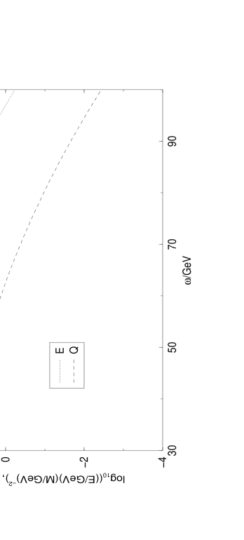
Figure 11: Energy and charge versus $\omega$, $U=U_{3}(\phi)$

Figure 12: Energy-charge ratio versus $\omega$, $U=U_{3}(\phi)$

Figure 13: Energy versus charge, $U=U_{3}(\phi)$

The numerical studies of these three types of potentials show different behaviour of charge and energy with changing $\omega$ for each type. As analytical results in the previous section showed the behaviour in the thick-wall limit depends critically on the power of the next to leading term. The logarithmic potential also shows a different kind of behaviour in the thick-wall limit. The question of stability of Q-balls in the thick wall-limit is hence strongly dependent on the exact form of the potential.

4 Q-ball evaporation

In realistic theories where the $\phi$-field couples to other fields the simple criterion for absolute stability $E<mQ$ no longer holds (it is still obviously true for $\phi$ decays). Here we discuss a decay mode to massless fermions. The evaporation of Q-balls to neutrinos was discussed in detail in [21]. It was shown that for a large Q-ball with a step-function boundary there exists an upper bound of the evaporation rate per unit area.

We follow closely the approach described in [21]. This is a leading order semi classical approximation where massless fermions are considered in the presence of a classical field, the Q-ball background. Since the Dirac sea is filled inside the Q-ball, evaporation can only progress through the Q-ball surface and is hence proportional to the area of the Q-ball. Evaporation progresses through pair-production at the Q-ball surface so that each pair produced decreases the charge of the Q-ball by two (e.g. a lepton number carrying ball could evaporate into neutrinos so that $\Delta L=2$ for each pair of neutrinos produced).

The Lagrangian density is given by

$$\mbox{$$}{\cal L}=\partial_{\mu}\phi^{*}\partial^{\mu}\phi-U(\left|\phi\right|)+\psi^{\dagger}(i\partial_{0}+i\sigma\cdot\nabla)\psi-ig\phi\psi^{\dagger}\sigma_{2}\psi^{*}+ig\phi^{*}\psi^{T}\sigma_{2}\psi,\vspace{\undereqskip}$$ (50)

where $\psi$ is a two component Weyl spinor corresponding to the fermion field, $\phi$ is the Q-ball scalar field and $\sigma$ are the Pauli matrices. The equations of motion are

$$\mbox{$$}(i\partial_{0}+i\sigma\cdot\nabla)\psi-g\phi\chi = 0$$

$$(i\partial_{0}-i\sigma\cdot\nabla)\chi-g\phi^{*}\psi = 0,\vspace{\undereqskip}$$ (51)

where $\chi=i\sigma_{2}\psi^{*}$ is a Weyl spinor. As in [21] we choose normal modes such that $\psi\sim e^{[-({\omega\over 2}+\omega^{\prime})it]}$ and $\chi\sim e^{[-(-{\omega\over 2}+\omega^{\prime})it]}$. With this choice the field equations become

$$\mbox{$$}({\omega\over 2}+\omega^{\prime}+i\sigma\cdot\nabla)\psi-g\phi\chi = 0$$

$$(-{\omega\over 2}+\omega^{\prime}-i\sigma\cdot\nabla)\chi-g\phi\psi = 0.\vspace{\undereqskip}$$ (52)

The eigensolutions to these equations can be found using spherical spinors. We make the ansatz

$$\mbox{$$}\psi = g_{1}(r)\Omega_{jlm}+if_{1}(r)\Omega_{jl^{\prime}m}$$

$$\chi = g_{2}(r)\Omega_{jlm}+if_{2}(r)\Omega_{jl^{\prime}m},\vspace{\undereqskip}$$ (53)

where $\Omega_{jlm},\ \Omega_{jl^{\prime}m}$ are spherical spinors [22],

$$\mbox{$$}\Omega_{j,\underbrace{\scriptstyle{j-1/2}}_{l},m} = {\sqrt{j+m\over 2j}Y_{l,m-1/2}\choose\sqrt{j-m\over 2j}Y_{l,m+1/2}}$$

$$\Omega_{j,\underbrace{\scriptstyle{j+1/2}}_{l},m} = {-\sqrt{j-m+1\over 2j}Y_{l,m-1/2}\choose\sqrt{j+m+1\over 2j+2}Y_{l,m+1/2}},\vspace{\undereqskip}$$ (54)

$Y_{lm}$ are spherical harmonics, $j$ and $m$ are the angular momentum quantum numbers and $l^{\prime}=2j-l$ and $j=l\pm{1\over 2}$.

Substituting the ansatz into the field equations (4) the radial equations are easily found (we set $g=1$):

$$\mbox{$$}({\omega\over 2}+\omega^{\prime})g_{1}(r)+f_{1}^{\prime}(r)-f_{1}(r){{3\over 2}+j\over r} = \phi(r)g_{2}(r)$$

$$({\omega\over 2}+\omega^{\prime})f_{1}(r)-g_{1}^{\prime}(r)-g_{1}(r){{1\over 2}-j\over r} = \phi(r)f_{2}(r)$$ (55)

$$(-{\omega\over 2}+\omega^{\prime})g_{2}(r)+f_{2}^{\prime}(r)+f_{2}(r){{3\over 2}+j\over r} = \phi(r)g_{1}(r)$$

$$(-{\omega\over 2}+\omega^{\prime})f_{2}(r)+g_{2}^{\prime}(r)+g_{2}(r){{1\over 2}-j\over r} = \phi(r)f_{1}(r).\vspace{\undereqskip}$$

We must now solve these equations with appropriate boundary conditions. Near the origin $r=0$ we can approximate the Q-ball potential with a constant, $\phi(r)=\phi_{0}$. In a suitable basis the radial equations decouple and an analytical solution can be found:

$$\mbox{$$}g_{1}^{0}(r) = A_{1}(\eta+\alpha)\eta_{1}j_{l_{-}}(\eta_{1}r)+A_{2}(\eta-\alpha)\eta_{2}j_{l_{-}}(\eta_{2}r)$$

$$f_{1}^{0}(r) = A_{1}(\omega+\alpha)\eta_{1}j_{l_{+}}(\eta_{1}r)+A_{2}(\omega-\alpha)j_{l_{+}}(\eta_{2}r)$$ (56)

$$g_{2}^{0}(r) = A_{1}g\phi_{0}\eta_{1}j_{l_{-}}(\eta_{1}r)+A_{2}g\phi_{0}\eta_{2}j_{l_{-}}(\eta_{2}r)$$

$$f_{2}^{0}(r) = A_{1}g\phi_{0}\eta_{1}j_{l_{+}}(\eta_{1}r)+A_{2}g\phi_{0}\eta_{2}j_{l_{+}}(\eta_{2}r),\vspace{\undereqskip}$$

where $l_{\pm}=j\pm{1\over 2}$, $\alpha=\sqrt{\omega^{\prime 2}-g^{2}\phi_{0}^{2}}$ and $\eta_{1,2}={\omega^{\prime}\over 2}\pm\alpha$. Here the divergent part (at the origin) of the general solutions has been omitted to keep the wave functions normalizable at $r=0$. Far away from the Q-ball surface $\phi=0$ and the equations of motion decouple into two pairs. An analytical solution can again be found:

$$\mbox{$$}g_{i}^{\infty}(r) = A_{i}k_{i}h^{(1)}_{l_{-}}(k_{i}r)+B_{i}k_{i}h^{(2)}_{l_{-}}(k_{i}r)$$

$$f_{i}^{\infty}(r) = A_{i}k_{i}h^{(1)}_{l_{+}}(k_{i}r)+B_{i}k_{i}h^{(2)}_{l_{+}}(k_{i}r),\vspace{\undereqskip}$$ (57)

where $i=1,2$, $h^{(i)}$ are the spherical Hankel functions and $k_{1,2}={\omega\over 2}\pm\omega^{\prime}$. From these we can identify the in- and out-moving waves since $h^{(1)}\sim e^{ir}$ and $h^{(2)}\sim e^{-ir}$. Solving for the coefficients $A_{i}$ and $B_{i}$ we get

$$\mbox{$$}A_{i} = {1\over k_{i}}{g_{i}^{\infty}(r)h^{(2)}_{l_{+}}(k_{i}r)-f_{i}^{\infty}(r)h^{(2)}_{l_{-}}(k_{i}r)\over h^{(1)}_{l_{-}}(k_{i}r)h^{(2)}_{l_{+}}(k_{i}r)-h^{(1)}_{l_{+}}(k_{i}r)h^{(2)}_{l_{-}}(k_{i}r)}$$

$$B_{i} = {1\over k_{i}}{g_{i}^{\infty}(r)h^{(1)}_{l_{+}}(k_{i}r)-f_{i}^{\infty}(r)h^{(1)}_{l_{-}}(k_{i}r)\over h^{(2)}_{l_{-}}(k_{i}r)h^{(1)}_{l_{+}}(k_{i}r)-h^{(2)}_{l_{+}}(k_{i}r)h^{(1)}_{l_{-}}(k_{i}r)}.\vspace{\undereqskip}$$ (58)

The evaporation rate can be calculated assuming that there is no incoming $\chi$ wave since then all the reflected $\chi$ flux must have been transmutated. From the transmutation coefficient $T$ the evaporation rate can be calculated [21]:

$$\mbox{$$}{dQ\over dt}=\sum_{j}\int_{0}^{\omega/2}{dk\over 2\pi}(2j+1)|T(k,j)|^{2}.\vspace{\undereqskip}$$ (59)

Here it is worth noting another result obtained in [21],

$$\mbox{$$}|T(k_{+},j)|=|T(k_{-},j)|\leq 1.\vspace{\undereqskip}$$ (60)

Assuming that the potential $U(\phi)$ scales as $U(s\phi)=s^{2}U(\phi)$, we note that under the transformation $\phi\rightarrow s\phi$, $\psi\rightarrow s\psi$, $g\rightarrow s^{-1}g$ the Lagrangian (50) transforms as ${\cal L}\rightarrow s^{2}{\cal L}$ so that the evaporation rate is invariant. Assuming as before a potential of the form (47) we note that the evaporation rate is invariant if $b$ scales as $b\rightarrow s^{-2A}b$.

In [21] the step-function boundary was considered in the large R limit. The calculation for any R is easily done by matching the in and out solutions (4,4). Assuming that there is no incoming $\chi$ flux, all the reflected $\chi$ waves must have then been transmutated. Identifying the coefficients $A_{i},\ B_{i}$ with the incoming, reflected and transmutated waves, the transmutation rate can be calculated in a straightforward way. The resulting expression is quite lengthy and is not presented here.

The maximum evaporation rate per unit area in the $R\rightarrow\infty$ limit was calculated in [21] by trading the angular momentum variable $j$ for a linear momentum variable and using relation (60). The maximum evaporation rate in this limit is given by

$$\mbox{$$}({dQ\over dAdt})_{\rm{max}}={\omega^{3}\over 192\pi^{2}}.\vspace{\undereqskip}$$ (61)

We have plotted the evaporation rates per unit area as a fraction of $({dQ\over dAdt})_{\rm{max}}$ for a number of $R$’s in Fig. 14.

Figure 14: Evaporation rates for a step-function boundary

Obviously the evaporation rate is strongly dependent on R and it approaches the limiting profile given in [21]. From the Fig. 14 it can be seen that the evaporation rate per unit area first increases with $R$ for all $g\phi_{0}/\omega$ until it reaches a maximum. Then the maximum value slowly starts to decrease and shift towards smaller $g\phi_{0}/\omega$ while a “bump” develops around $\log(g\phi_{0}/\omega)\sim-0.5$. The different types of behaviour at small and large $g\phi_{0}/\omega$ is due to the presence of the $\exp(i\sqrt{\omega^{\prime 2}-g^{2}\phi_{0}^{2}}R)$-term in the matching process of the wave functions in- and outside the Q-ball. When $\omega^{\prime}>g\phi_{0}$ the wave-function consists of oscillatory functions compared to $\omega^{\prime}<g\phi_{0}$ when exponentially growing and decaying parts are present. As $R$ increases this effect becomes more pronounced and the evaporation rate tends to a constant more quickly as $g\phi_{0}/\omega$ increase. The slightly rough features at small $g\phi_{0}/\omega$ are also due to the strong oscillatory $R$ dependence.

In a realistic case a step-function is not always a good approximation. It approximates a thin-walled Q-ball well but for a thick-walled Q-ball its accuracy may be questioned. The profile a thick-walled Q-ball is significantly different from a step-function and furthermore its radius is not well defined. To model a thick-walled Q-ball with a step-function Q-ball one could for example choose the charges to be equal. This would still leave the radius and the value of the field inside the ball arbitrary. One should then define the Q-ball boundary to obtain a radius and hence obtain $\phi_{0}$. The accuracy of such an approximation can be questioned especially in the case of very thick-walled Q-balls.

We have examined the evaporation rates numerically for realistic Q-balls profiles (in addition to checking that the purely numerical calculation recovers the results for a step-function boundary). This is done by solving the equations (4) numerically for a given profile. The profiles have been calculated from the different types of potentials, $U_{i}(\phi),\ i=1,2,3$.

The numerical solution is found using the fact that asymptotically the Q-ball profile at the origin is flat and can be approximated with a constant. The analytical solution is then given by (4). Far away from the Q-ball surface the potential is zero and the solution there is given by (4). The problem then reduces to finding the right initial conditions to obtain a solution from which we can deduce the transmutation coefficient i.e.we must choose $A_{1}$ and $A_{2}$ in (4) such that far away from the Q-ball there is no incoming $\chi$-wave. The coefficients for the incoming and reflected $\psi$-wave and for the transmutated $\chi$-wave can then be found by using (4).

We have calculated the evaporation rate (59) for a number of $\omega$:s in the three different potentials. These are presented in Figures 15, 16 and 17 as a function of charge. Note that here the evaporation rate is not given as a fraction of the maximum rate and is the total evaporation rate (instead of the evaporation rate per unit area). We have only plotted the evaporation rates for a parameter range where Q-balls are stable with respect to decay into $\phi$-scalars.

Figure 15: Evaporation rate ${dQ\over dt}$ versus $\log Q$, $U=U_{1}(\phi)$ ($m_{1}=1$)

Figure 16: Evaporation rate ${dQ\over dt}$ versus $\log Q$, $U=U_{2}(\phi)$ ($m_{1}=1$)

Figure 17: Evaporation rate ${dQ\over dt}$ versus $\log Q$, $U=U_{3}(\phi)$

From the figures we see that at large Q the evaporation rate decreases with increasing Q. This holds for the whole of the studied parameter range for all the potentials so that a Q-ball will evaporate faster as it decreases in size. The calculation is quite time consuming and requires high numerical accuracy in choosing $A_{1}$ and $A_{2}$ correctly. This fact is evident in the slight non-smoothness present in the figures due to numerical inaccuracies during the computation.

We have fitted a curve ${dQ\over dt}=\alpha(\log Q)^{\beta}+\gamma$ through the points in each case. These fits are presented in the corresponding figures.

It is cosmologically interesting to estimate the evaporation times, especially for the realistic potential $U_{3}(\phi)$. Let us consider a typical Q-ball in the logarithmic potential that is stable with respect to scalar decays. For a Q-ball to survive past the electroweak (EW) phase transition we can estimate that its lifetime must be $\sim 10^{-12}\ \textrm{s}\sim 10^{12}\ \textrm{(GeV)}^{-1}$. From the Fig. 17 we can estimate that the evaporation rate is $\sim 10\ \textrm{GeV}$ so that its charge must be at least $10^{13}$ for it to evaporate for $10^{-12}$ s. However, from Fig. 13 we see that scalar decays begin at about $Q\sim 10^{24}$. The lifetime of a typical Q-ball with charge of the order of $\sim(M/\textrm{(GeV)})^{2}$ is then sufficiently long for it to survive past the EW phase transition. On the other hand a Q-ball with charge $\sim 10^{24}$ will evaporate in $\sim 10^{23}\ \textrm{(GeV)}^{-1}\sim 10^{-2}$ s so that Q-balls are no longer present in the universe.

We can now estimate the emitted power in Q-ball evaporation. Writing

$$\mbox{$$}W={{dE}\over{dt}}={{\partial E}\over{\partial Q}}{{dQ}\over{dt}}\vspace{\undereqskip}$$ (62)

so that we see that ${{\partial E}\over{\partial Q}}$ must be considered as $E$ decreases. From the Figures 7, 10 and 13 we can see that in the stable regime, ${{\partial E}\over{\partial Q}}<m$ in all the three cases. The emitted power then increases until scalar decays begin. Especially in the case of potential $U_{2}(\phi)$ the emitted power can be quite large. However, it must be kept in mind that this calculation is based on a semi classical analysis and very small Q-balls should be analyzed quantum mechanically.

In analyzing the decay of Q-balls in the early universe one should also consider dissociation and dissolution [11]. These are due to the presence of a thermal background in the early universe. To evade the dissociation and dissolution of typical Q-balls produced from an AD-condensate, an upper bound for the reheating temperature of $\sim 10^{3-5}$ GeV has been derived [11].

5 Conclusions

Q-ball properties have been studied using both analytical and numerical methods. Analytically we have examined the stability and charge of Q-balls in the limit where $\omega\rightarrow m$. In this thick wall limit we have derived conditions for stable Q-balls to exist in a potential that can be expressed as powers of $\phi$ in the limit of small $\phi$. It was shown that stability depends on the dimension of the theory as well as on the power of the next to leading term in the small $\phi$ limit. These results confirm previous results and present a method of analyzing the stability of Q-balls when $\omega\rightarrow m$.

Three different types of potentials have been studied numerically. These calculations show how stability in the thick-wall limit is strongly dependent on the exact form of the scalar potential. Numerical examinations show different types of behaviour in the charge versus energy plot for all of the three potentials. Furthermore, numerical work agrees with the analytical results. In studying the potential resulting from a MSSM D-flat direction with supergravity induced SUSY breaking we note that at least for the studied parameter values, the stability of Q-balls requires that $Q\sim 10^{24}$. This quite a large number shows that one should be careful to check whether the Q-balls formed in the early universe will survive scalar decays for a given set of parameters if Q-balls are to be cosmologically significant.

The evaporation of Q-balls was considered for a thin-walled Q-ball and for realistic Q-ball profiles. We have recreated a previous result calculated for a semi-infinite ball. For realistic Q-ball profiles it was shown that as Q-balls lose their charge due to evaporation they evaporate at a faster rate. Evaporation then progresses at an accelerating rate until scalar decays begin. The emitted power also increases with decreasing charge so that Q-balls disappear in a burst of particles. Cosmologically this means that if the universe was dominated by Q-balls at some point in its evolution, there will be some inhomogeneity introduced by the evaporation process. For example, if the baryon asymmetry or dark matter was stored in Q-balls, inhomogeneity will be introduced as the Q-balls evaporate. This inhomogeneity could be cosmologically significant and possibly observable.

References

• [1] T. Lee and Y. Pang, Phys.Β Rev.Β 221 (1992) 251.
• [2] S. Coleman, Nucl.Β Phys.Β B262 (1985) 263.
• [3] K. Lee et al., Phys.Β Rev.Β D39 (1989) 1665.
• [4] H. P. Nilles, Phys.Β Rev.Β 110 (1984) 1.
• [5] M. Dine, L. Randall and S. Thomas, Nucl.Β Phys.Β B458 (1996) 291.
• [6] A. Kusenko, Phys.Β Lett.Β B404 (1997) 285.
• [7] K. Enqvist and J. McDonald, Phys.Β Lett.Β B425 (1998) 309.
• [8] A. Kusenko and M. Shaposhnikov, Phys.Β Lett.Β B418 (1998) 46.
• [9] I. Affleck and M. Dine, Nucl.Β Phys.Β B249 (1985) 361.
• [10] K. Enqvist and J. McDonald, hep-ph/9908316.
• [11] K. Enqvist and J. McDonald, Nucl.Β Phys.Β B538 (1999) 321.
• [12] S. Dimopoulos et al., Nucl. Phys. Proc. Suppl. A52 (1997) 38.
• [13] G. Dvali, A. Kusenko and M. Shaposhnikov, Phys.Β Lett.Β B417 (1998) 99.
• [14] A. Kusenko, Phys.Β Lett.Β B405 (1997) 108.
• [15] A. Kusenko et al., Phys.Β Lett.Β B423 (1998) 104.
• [16] A. Kusenko et al., PhysΒ Rev.Β Lett.Β 80 (1998) 3185.
• [17] S. Ahlen et al., PhysΒ Rev.Β Lett.Β 69 (1992) 1860.
• [18] I. Belolaptikov et al., astro-ph/9802223.
• [19] S. Coleman, V. Glaser and A. Martin, Comm. Math. Phys. 58 (1978) 211.
• [20] K. Enqvist and J. McDonald, Phys.Β Lett.Β B440 (1998) 59.
• [21] A. Cohen et al., Nucl.Β Phys.Β B272 (1986) 301.
• [22] W. Greiner, Relativistic Quantum Mechanics, Springer-Verlag 1990.