Color Screening Effects on Hadronization in Relativistic Heavy Ion Collisions

Abstract

The effects of color screening on the hadronization of a parton plasma into a hadron gas are examined at the energies of the relativistic heavy ion collider. It is found to have the tendency to prevent hadronization and therefore delaying the conversion of the partons into a hadron gas. Because of the continual expansion, the resulting hadron gas number densities are lower when screening is included. This should reduce the hadronic noise to genuine signals of the quark-gluon plasma. In this sense, color screening is favorable and should be included in numerical models. In any case, we advocate that numerical models should allow the confining forces and color screening to act on each other so as to undergo the phase transition in a natural way. Hadronization is also shown to seriously disrupt parton equilibration and is yet another reason why full parton chemical equilibration should not be expected.

PACS: 25.75.-q, 24.85.+p, 12.38.Mh, 12.38.Bx NUC-MINN-99/11-T

I Introduction

The Relativistic Heavy Ion Collider (RHIC) at Brookhaven will be put into operation in the imminent future. The primary aims of the experiments to be conducted at the new collider are to show that deconfined matter can indeed exist under extreme conditions and also to uncover its properties. These are no easy tasks since the high energy per nucleon combined with the multi-particle initial states lead to the possibility of the many particles to undergo multiple interactions. The resulting interactions are far more complicated than what have been studied so far, not to mention the complex interactions that will take place in a region of sizable spatial extent and temporal duration. These are novel aspects for scattering experiments. This is especially true of the time evolution, which is usually not even under consideration in $e^{+}e^{-}$ annihilations or proton-antiproton collision experiments due to the short duration of these processes. The final states or the end products are therefore the main concerns in these cases. When facing many-body processes, numerical models are very essential. This is even more so in heavy ion collisions than in $e^{+}e^{-}$ annihilations or proton-antiproton collisions when the actual time evolution of the collisions becomes important. When modeling high energy nuclear interactions, it is necessary therefore to follow the partons through into the hadron phase till the very end. The transition from partons into hadrons is a considerable challenge. This is so because exactly how quarks and gluons are bounded into hadrons is not well understood. If one is only interested in the final states, one can proceed as in [1, 2] for $e^{+}e^{-}$ annihilation into hadrons since the hadronization takes place after the primary jet partons have a chance to evolve into parton showers through time-like parton branching. So this is to a certain extent similar to the situation of that in a gas of partons. The major difference is the latter exist in a much denser medium and there is color screening whereas the former is essentially hadronization in a vacuum. So one should keep well in mind of these differences and include as much of these in any attempts at modeling parton to hadron transitions in a QCD medium. As far as we can tell, there is no attempt in this direction in any realistic model. In [3], attempt was made to incorporate hadronization in the parton cascade model (PCM) [4, 5, 6] but the hadronization process was essentially the same as that used in $e^{+}e^{-}$ in [2] and therefore medium effects on hadron formation have been totally neglected. Note that one could also study the transition to hadrons by using textbook type approaches [7] or by concentrating entirely on the macroscopic properties such as bubble formation and growth [8, 9, 10], but by doing so most details that we are interested in will be hidden from view in such coarse-grain approaches.

In our previous investigations in [11], we found that the average interaction strength in a parton plasma created in the wake of the initial hard collisions at RHIC or at the Large Hadron Collider at CERN tended to increase monotonically in time or the interactions tended to become stronger and stronger with time. One of the consequences of this is that the screening mass, or more generally, the medium generated masses calculated at leading order also increases monotonically in time at least at RHIC and within the duration that we investigated, the screening length therefore decreases. In Fig. 1, we plotted the time development of the square of the screening mass $m_{D}$ and medium generated quark mass $m_{q}$ and also the screening length $l_{D}$, all at leading order at RHIC which was calculated from the time evolution of the parton plasma in [11]. They clearly show the above mentioned behavior. The actual screening length at the end of the run when the temperature estimates fell to about 200 MeV was about 0.4 fm. This is comparable to the size of the most common hadrons. If the leading order results are anything to go by, this is not particularly good for hadronization if it really does occur at this time. To see what are the implications beyond leading order, we must turn to lattice calculations since perturbative calculation at the next-to-leading order required the introduction of the non-perturbative color magnetic mass as an infrared cutoff [12]. In ref. [13] the Debye screening mass $m_{D}$ was calculated for SU(N=3) on the lattice up to the term at ${\cal O}(g^{3})$ in the linear power dependence on $g$ but each term had a non-perturbative coefficient which may or may not have logarithmic, non-analytic $g$-dependence. It was found that in a large range of temperatures near and above the phase transition temperature $T_{c}$, it was several times larger than the leading order result $m_{D}^{\text{LO}}$. To be more precise,

$$m_{D}\;\simeq 3.3\;m_{D}^{\text{LO}}\;.$$ (1)

             

FIG. 1.: The time variation of (a) the medium masses at leading order and (b) the corresponding screening length from graph (a) at RHIC. The dashed line in graph (b) is if we used a factor of 3.3 to get the $m_{D}$ result evaluated up to ${\cal O}(g^{3})$ from lattice as discussed in the text.

From the equations

$$m_{D}^{\text{LO}} = (N/3+n_{f}/6)^{1/2}\,g\,T$$ (2)

$$g^{2}(\mu) = {{24\pi^{2}}\over{(11N-2n_{f})\ln\mu/{\Lambda_{\overline{\text{MS}}}}}}$$ (3)

$$\mu\;\; = 4\pi\;e^{-\gamma_{E}}\;T\;\mbox{\rm exp}\left({{-3c_{m}+4n_{f}\log 4}\over{22N-4n_{f}}}\right)$$ (4)

$$c_{m}\; = {{10N^{2}+2n_{f}^{2}+9n_{f}/N}\over{6N+3n_{f}}}$$ (5)

given in [13, 14], we can estimate the screening length at various temperatures. Using two flavors of quarks $n_{f}=2$ and $\Lambda_{\overline{\text{MS}}}=234$ MeV, $m_{D}^{\text{LO}}=487.94$ MeV at $T=200$ MeV and $m_{D}^{\text{LO}}=398.63$ MeV at $T=150$ MeV. The screening length derived from the value of the non-perturbative $m_{D}$ up to ${\cal O}(g^{3})$ would then be $l_{D}=0.123$ fm at $T=200$ MeV and $l_{D}=0.150$ fm at $T=150$ MeV. These are really small values when compared to even the smallest of hadrons. We must emphasize here once again that although these results are up to ${\cal O}(g^{3})$, they are not perturbative because as we mentioned above already, the coefficient at each power of $g$ is non-perturbative. In Fig. 1 (b), the leading order $m_{D}^{LO}$ in (a) was given a factor of 3.3 to arrive at the dashed curve to show the approximate small size of the would-be actual screening length if the screening mass was properly calculated non-perturbatively to beyond the leading order. Remember that the color screening property of a high energy and dense system of color charges is to reduce the color field exponentially within a distance of the screening length $l_{D}$. Thus color binding forces responsible for hadronizing, for example, the parton shower in $e^{+}e^{-}$ annihilation would be weakened in a dense QCD parton medium. The conversion of partons into hadrons therefore cannot occur freely in heavy ion collisions. In fact, most hadrons cannot survive in an environment with the range of values of $l_{D}$ that were shown above. So if we impose by force the hadronization time to be at any moment with $\tau<3.5$ fm without any regard to color screening, it would not make any sense physically. The best way to simulate hadronization, in our opinion, seems to be to let screening and the confining forces act against each other and not to impose a priori a specific temperature or density at which hadronization must occur. The worse is of course to neglect color screening entirely. In this paper, we attempt to show the effects of color screened QCD medium has on hadronization and compare and contrast it with that without color screening or that occurring essentially in a vacuum. We will do this by letting the system decide by itself when to hadronize.

II Time evolution equations with hadronization

A Basic Assumptions, Simplifications and Hadronization Mechanism

Based on our time-evolution scheme developed in [11, 15, 16] for a parton plasma which we reported in [17] and applied to study several particle productions in [18], we now try to incorporate hadronization into the time evolution equations. In order to do this, we introduce the following simplifications.

• The focus is in a region within a thin slice perpendicular to the beam direction in the central region.

• This region is spatially homogeneous.

• There is only longitudinal Bjorken-like expansion within this region.

• There is boost invariance in the longitudinal or beam direction.

• Surface effects will not be considered or the region of interest will be the central core well away from the surface.

• Hadrons and resonances are formed by $q\,\bar{q}^{\prime}$ only, where $q,q^{\prime}=u,d$ or $s$.

• Resonances only undergo two-body decay.

• For hadrons, only $\pi$’s and $K$’s are considered.

• Only orbital angular momentum $L\leq 1$ are allowed.

The first four simplifications, i)–iv), are quite common and were used extensively in equilibration or hydrodynamics studies of the quark-gluon plasma and hydrodynamics studies of a hadron gas. Indeed, we relied heavily on them in our previous investigations of the time evolution of the parton plasma [11, 15, 16]. The v) is there because the surface regions are less interesting since color screening will be most important in the center where the parton density is highest. Near the surface hadrons will be evaporating away from the system, whereas at the center hadronic bubbles will form instead. Although we do not explicitly use this type of macroscopic language, our focus in this paper will be on the latter because color screening is less relevant near the surface. The vi) and the vii) were used in the studies of $e^{+}e^{-}$ annihilations [1, 2] and we introduce viii) for reasons to be discussed below and also for the practical reason to reduce the time for computation. The last is purely there to avoid having to consider too many possibilities.

Recalling that the main ingredients of our scheme consist of using a reduced form of the Boltzmann equation introduced by Baym [19] for the particle distribution $f_{i}$ and for the collision terms $C_{i}$, we used the relaxation time approximation as well as constructing them explicitly from parton interactions. The main time evolution equations for the partons thus appeared as

$${{\mbox{d}f_{i}^{\text{p}}}\over{\mbox{d}\tau}}\,\Big{|}_{p_{z}\tau=\text{constant}}\;=-\;{{f_{i}^{\text{p}}-f^{\text{p}}_{i\;eq}}\over{\theta_{i}^{\text{p}}}}\;=\;C_{i}^{\text{p}}$$ (6)

where $i=g,q,\bar{q}$. The double construction of $C_{i}^{\text{p}}$ for the parton collisions, hence the superscript p, is necessary to close the equations in order to be able to solve for the time-dependent parameters of the model. These will give us several time-dependent particle distributions $f^{\text{p}}_{i}$ which completely describe the time evolution of our partonic system.

Here we very briefly recall the steps to arrive at the solution of Eq. (6). This reduced Boltzmann equation has the advantage that a partial solution in analytic form can be readily written down. That is

$$f^{\text{p}}_{i}(p,\tau)=f^{\text{p}}_{0\;i}(p,\tau)\;\mbox{\rm exp}{(-x^{\text{p}})}+\int^{x^{\text{p}}}_{0}d{x^{\text{p}}}^{\prime}\;\mbox{\rm exp}{({x^{\text{p}}}^{\prime}-x^{\text{p}})}\;f^{\text{p}}_{\text{eq}\;i}(p,T^{\text{p}}_{\text{eq}\;i}(\tau^{\prime}),\tau^{\prime},\tau)$$ (7)

where

$$x^{\text{p}}(\tau)=\int^{\tau}_{\tau_{0}}d\tau^{\prime}/\theta^{\text{p}}_{i}(\tau^{\prime})$$ (8)

and $f^{\text{p}}_{0\;i}$ is the initial distribution for parton species $i$ at $\tau_{0}$. All there remains is to determine the parameters $T^{\text{p}}_{\text{eq}}(\tau)$ and $\theta^{\text{p}}(\tau)$ for a complete solution. For this purpose, the perturbative construction of the collision terms was made. The two parameters were solved by converting any integral over $\tau$ into a discrete sum as discussed in [15]. For example, an integral function $G(\tau)$ would be discretized as

$$G(\tau)=\int^{\tau}_{\tau_{0}}d\tau^{\prime}\tilde{G}(\tau,\tau^{\prime})\;\;\Longrightarrow\;\;G(\tau_{n})=\sum^{n-1}_{i=0}\Delta\tau\;\tilde{G}(\tau_{n},\tau_{i})\;.$$ (9)

Therefore provided that $\tilde{G}$ and any time-dependent parameters that it might have are known at all $\tau<\tau_{n}$, $G(\tau_{n})$ is determined completely. When this method is applied to the distribution functions $f^{\text{p}}_{i}$, they are determined at time $\tau$ if the parameters $\theta$ and $T_{\text{eq}}$ are known at all moments before $\tau$. As a consequence, the medium masses, energy densities, number densities, perturbatively constructed collision terms etc. at any moment can be calculated by knowing the parameters of all earlier time-steps. The parameters of the next time-step are found by equating the relaxation time approximation and the perturbatively constructed collision terms and solving the resulting fourth degree polynomials. These steps are for solving Eq. (6) for partons. When hadrons are introduced in the later sections and given their own transport equations, only the last step will be different. Instead of finding solutions to polynomials, we will be doing that to equations involving Bessel functions.

To include hadronization in our model, one has to have a scheme. There are at least three different schemes that are being used in the studies of $e^{+}e^{-}$ annihilations [20], namely string fragmentation, independent parton fragmentation and parton clustering. Since we prefer the parton language, we will not choose the first scheme. Of the remaining two, independent parton fragmentation [21, 22] tends to always end with a parton so this scheme by itself cannot convert a parton gas completely into hadrons. The more suitable scheme therefore is the third scheme of parton clustering into hadrons [1, 2]. It may be that the combination of the second and the third is the more correct parton based picture but we will use only one scheme for simplicity.

To form hadrons via clustering, any number of partons can in principle participate in any one single cluster provided that they form a color singlet. It has to be said that the binding of a number of partons into a color singlet cluster does not directly result in the observed hadrons, rather they will appear as the decay products of the first formed cluster. For hadrons at least and it is reasonable to assume the same to be true for the first formed resonance cluster, the probability of a hadron in a state with many constituents is much less than if it is in the valence state. So instead of allowing any number of partons to form any one cluster, we will only allow two, that is a quark and an antiquark to keep the scheme simple. This is the reasoning behind simplification vi) above. There is, however, an obvious obstacle to this simple scheme. The parton plasma is well known to be gluon dominated because of the small $x$ growth of the gluon distribution in the nucleon. Barring the possibility of forming any glueball mesons, the gluons must be converted into fermions somehow to fit in with our simple hadronization scheme. Of course there is always the perturbative conversion of gluons into quark-antiquark pairs but it is a too inefficient process. Quite similarly in the studies or modeling of $e^{+}e^{-}$ annihilations, it was also found that the time-like branching of gluon into quark-antiquark was much less probable than that of branching into gluon, so it was necessary to resort to some non-perturbative mechanism to ensure that the parton branching always ends in a quark-antiquark pair. A non-perturbative gluon splitting mechanism into quark-antiquark was introduced in [1] for this purpose. Here we will therefore also introduce such a process. However, the conversion mechanism that we will use below in the next section can only be similar in essence, but not in detail to that used in $e^{+}e^{-}$ annihilation. This is so because the parton shower created from the parton branching consists entirely of off-shell time-like partons whereas the partons in the parton plasma are essentially massless and on-shell. We will discuss this further below.

B Parton-Hadron Conversion

By bringing in all the afore-mentioned mechanisms to complete our simple hadronization scheme, our time evolution equations for partons given in Eq. (6) become

$${{\mbox{d}f_{i}^{\text{p}}}\over{\mbox{d}\tau}}\,\Big{|}_{p_{z}\tau=\text{constant}}\;=-\;{{f_{i}^{\text{p}}-f^{\text{p}}_{i\;eq}}\over{\theta_{i}^{\text{p}}}}\;=\;C_{i}^{\text{p}}+C^{\text{p}}_{i\;g\rightarrow q}+C^{\text{p}}_{i\;p\rightarrow h}\;.$$ (10)

We have not included the possibility of parton-hadron interactions and will not do so in this paper. By introducing hadrons into the system, one time evolution equation must be included for each hadron type. Using the same relaxation time approximation for the partons as for hadrons, we have the following time evolution equations for the hadrons

$${{\mbox{d}f_{i}^{\text{h}}}\over{\mbox{d}\tau}}\,\Big{|}_{p_{z}\tau=\text{constant}}\;=-\;{{f_{i}^{\text{h}}-f^{\text{h}}_{i\;eq}}\over{\theta_{i}^{\text{h}}}}\;=\;C^{\text{h}}_{i\;p\rightarrow h}\;,$$ (11)

where $i=\pi,K$ since we only include pions and kaons, and the interactions amongst hadrons are also not considered because they are not our main focus here. The form of the parton collision terms $C_{i}^{\text{p}}$ can be found in [15, 16]. The new terms $C^{\text{p}}_{i\;g\rightarrow q}$, $C^{\text{p}}_{i\;p\rightarrow h}$ and $C^{\text{h}}_{i\;p\rightarrow h}$ introduced here will be given and explained below.

Considering only three flavors and allowing only $q\bar{q}^{\prime}$ to form color singlet resonance clusters, the resulting clusters can have their constituents in different spin and angular momentum combinations. This together with the flavor of the fermion constituents put them into definite parity, C-parity, angular momentum and isospin state. These must be conserved in the subsequent strong decay into observable hadrons. Because of simplification vii) and viii) and the conservation laws, with only two pseudo-scalars in the decay products means that not all possibilities of parity ${\cal P}$, C-parity, spin $S$ and orbital $L$ or total $J$ angular momentum of the resonances are possible. Using the $J^{{\cal P}(C)}$ notation, where the $C$ only applies when we have flavor neutrality or equivalently when the resonance is an eigenstate of charge conjugation operator $C$, resonance clusters can only be found in any of the $1^{-(-)}$, $0^{+(+)}$ or $2^{+(+)}$ under the restrictions that we imposed.

For any given $q\bar{q}^{\prime}$, if the kinematics allows it, we will assume that there are no preferences in the binding of the pair into each of the three possible cluster states given above. Thus for a number of $q\bar{q}^{\prime}$ at any moment, an equal portion of them at that moment will choose to form each of the possible resonances. Likewise, we use the same assumption for the subsequent decays of these resonances into each possible channel. For all kinematically allowed channels, equal number of any given kind of resonances at any moment will choose to go into each of the possible hadron pairs, although the conversion rate for different channels may not be the same due to other factors such as mass differences and the available phase space.

In the decay process, because we have assumed that both the resonance clusters and the mesons are formed of $q\bar{q}^{\prime}$, a pair of quark-antiquark has to be created. We allow $u,d$ or $s$ flavor to have equal chance to be created. One may object to this equal probability even for the $s$ quark because it is so much heavier than the light quarks. The reason that the same probability is assigned even to the strange flavor is because we prefer to let phase space takes over so that the smaller number of kaons in the final hadron abundance would be due entirely to the available phase space. The latter has a major role to play in the final particle abundances as was discovered by Hagedorn in the studies of large angle p-p collision in the 50’s. This has, following various events, led to the construction of the statistical bootstrap model [23, 24]. This is the basic reason why we choose to let phase space decide the hadron yields rather than introducing some ad hoc, uneven probability for any flavor of $q\bar{q}$ pair creation in the decay process. As to the rate of conversion of the partons into hadrons, it is controlled to a definite extent by isospin constraint. In Table I, Table IV and Table IV, we give the relative probabilities ${\cal F}_{q\bar{q}^{\prime}}^{hh^{\prime}}$ of any given $q\bar{q}^{\prime}$ with invariant mass $M$ to go through the three possible resonance cluster states and to end up as any of the possible final hadron pairs $hh^{\prime}$. Not all possibilities of fermion pairs are given, those not given have the same relative probabilities as their charge conjugated pairs.

TABLE I.: Relative probabilities ${\cal F}_{q\bar{q}^{\prime}}^{hh^{\prime}}$ of any $q\bar{q}^{\prime}$ to go through different clustering and into the decay channels indicated in parenthesis in the cluster invariant mass range $2\;m_{\pi}\leq M<m_{\pi}+m_{K}$.

$q\bar{q}^{\prime}\;\big{\backslash}\;{\cal F}_{q\bar{q}^{\prime}}^{hh^{\prime}}\big{\backslash}$ cluster $J^{{\cal P}(C)}$	$1^{-(-)}$	$0^{+(+)}$	$2^{+(+)}$
$u\;\bar{d}$	$1\;(\pi^{0}\;\pi^{+})$	$\emptyset$	$\emptyset$
$u\;\bar{u}$	$\frac{1}{3}\;(\pi^{+}\;\pi^{-})$	$\frac{1}{6}\;(\pi^{+}\;\pi^{-})$ , $\frac{1}{6}\;(\pi^{0}\;\pi^{0})$	$\frac{1}{6}\;(\pi^{+}\;\pi^{-})$ , $\frac{1}{6}\;(\pi^{0}\;\pi^{0})$
$d\;\bar{d}$	$\frac{1}{3}\;(\pi^{+}\;\pi^{-})$	$\frac{1}{6}\;(\pi^{+}\;\pi^{-})$ , $\frac{1}{6}\;(\pi^{0}\;\pi^{0})$	$\frac{1}{6}\;(\pi^{+}\;\pi^{-})$ , $\frac{1}{6}\;(\pi^{0}\;\pi^{0})$
$u\;\bar{s}$	$\emptyset$	$\emptyset$	$\emptyset$
$d\;\bar{s}$	$\emptyset$	$\emptyset$	$\emptyset$
$s\;\bar{s}$	$\emptyset$	$\emptyset$	$\emptyset$

If the QCD Lagrangian for three flavors could be rewritten into an effective one which contains terms that describe binding of, for example, $q\bar{q}^{\prime}$, $q\bar{q}^{\prime}g$, $q\bar{q}^{\prime}gg$, $\dots$ into hadrons and this Lagrangian is flavor blind, then the rate of our simplified parton-hadron conversion could be written with only three unknown transition matrix functions, which in general would have some mass dimensions. These functions would describe the isospin zero-to-zero, one-to-one and half-to-half confinement transitions. In Table IV, we give the isospin coefficients $\Upsilon_{q\bar{q}^{\prime}}^{hh^{\prime}}$ and the dependence of each transition on the three functions which are written as $\langle I=0|{\cal H}|I=0\rangle$, $\langle I=1|{\cal H}|I=1\rangle$ and $\langle I=1/2|{\cal H}|I=1/2\rangle$.

TABLE II.: Relative probabilities ${\cal F}_{q\bar{q}^{\prime}}^{hh^{\prime}}$ of any $q\bar{q}^{\prime}$ to go through different clustering and into the decay channels indicated in parenthesis in the cluster invariant mass range $m_{\pi}+m_{K}\leq M<2\;m_{K}$.

$q\bar{q}^{\prime}\;\big{\backslash}\;{\cal F}_{q\bar{q}^{\prime}}^{hh^{\prime}}\big{\backslash}$ cluster $J^{{\cal P}(C)}$	$1^{-(-)}$	$0^{+(+)}$	$2^{+(+)}$
$u\;\bar{d}$	$1\;(\pi^{0}\;\pi^{+})$	$\emptyset$	$\emptyset$
$u\;\bar{u}$	$\frac{1}{3}\;(\pi^{+}\;\pi^{-})$	$\frac{1}{6}\;(\pi^{+}\;\pi^{-})$ , $\frac{1}{6}\;(\pi^{0}\;\pi^{0})$	$\frac{1}{6}\;(\pi^{+}\;\pi^{-})$ , $\frac{1}{6}\;(\pi^{0}\;\pi^{0})$
$d\;\bar{d}$	$\frac{1}{3}\;(\pi^{+}\;\pi^{-})$	$\frac{1}{6}\;(\pi^{+}\;\pi^{-})$ , $\frac{1}{6}\;(\pi^{0}\;\pi^{0})$	$\frac{1}{6}\;(\pi^{+}\;\pi^{-})$ , $\frac{1}{6}\;(\pi^{0}\;\pi^{0})$
$u\;\bar{s}$	$\frac{1}{6}\;(\pi^{0}\;K^{+})$ , $\frac{1}{6}\;(\pi^{+}\;K^{0})$	$\frac{1}{6}\;(\pi^{0}\;K^{+})$ , $\frac{1}{6}\;(\pi^{+}\;K^{0})$	$\frac{1}{6}\;(\pi^{0}\;K^{+})$ , $\frac{1}{6}\;(\pi^{+}\;K^{0})$
$d\;\bar{s}$	$\frac{1}{6}\;(\pi^{0}\;K^{0})$ , $\frac{1}{6}\;(\pi^{-}\;K^{+})$	$\frac{1}{6}\;(\pi^{0}\;K^{0})$ , $\frac{1}{6}\;(\pi^{-}\;K^{+})$	$\frac{1}{6}\;(\pi^{0}\;K^{0})$ , $\frac{1}{6}\;(\pi^{-}\;K^{+})$
$s\;\bar{s}$	$\emptyset$	$\emptyset$	$\emptyset$

TABLE III.: Relative probabilities ${\cal F}_{q\bar{q}^{\prime}}^{hh^{\prime}}$ of any $q\bar{q}^{\prime}$ to go through different clustering and into the decay channels indicated in parenthesis in the cluster invariant mass range $2\;m_{K}\leq M$.

$q\bar{q}^{\prime}\;\big{\backslash}\;{\cal F}_{q\bar{q}^{\prime}}^{hh^{\prime}}\big{\backslash}$ cluster $J^{{\cal P}(C)}$	$1^{-(-)}$	$0^{+(+)}$	$2^{+(+)}$
$u\;\bar{d}$	$\frac{1}{6}\;(\pi^{0}\;\pi^{+})$ , $\frac{1}{6}\;(K^{+}\;\bar{K^{0}})$	$\frac{1}{3}\;(K^{+}\;\bar{K}^{0})$	$\frac{1}{3}\;(K^{+}\;\bar{K}^{0})$
$u\;\bar{u}$	$\frac{1}{6}\;(\pi^{+}\;\pi^{-})$ , $\frac{1}{6}\;(K^{+}\;K^{-})$	$\frac{1}{9}\;(\pi^{+}\;\pi^{-})$ , $\frac{1}{9}\;(\pi^{0}\;\pi^{0})$ ,	$\frac{1}{9}\;(\pi^{+}\;\pi^{-})$ , $\frac{1}{9}\;(\pi^{0}\;\pi^{0})$ ,
		$\frac{1}{9}\;(K^{+}\;K^{-})$	$\frac{1}{9}\;(K^{+}\;K^{-})$
$d\;\bar{d}$	$\frac{1}{6}\;(\pi^{+}\;\pi^{-})$ , $\frac{1}{6}\;(K^{0}\;\bar{K}^{0})$	$\frac{1}{9}\;(\pi^{+}\;\pi^{-})$ , $\frac{1}{9}\;(\pi^{0}\;\pi^{0})$ ,	$\frac{1}{9}\;(\pi^{+}\;\pi^{-})$ , $\frac{1}{9}\;(\pi^{0}\;\pi^{0})$ ,
		$\frac{1}{9}\;(K^{0}\;\bar{K}^{0})$	$\frac{1}{9}\;(K^{0}\;\bar{K}^{0})$
$u\;\bar{s}$	$\frac{1}{6}\;(\pi^{0}\;K^{+})$ , $\frac{1}{6}\;(\pi^{+}\;K^{0})$	$\frac{1}{6}\;(\pi^{0}\;K^{+})$ , $\frac{1}{6}\;(\pi^{+}\;K^{0})$	$\frac{1}{6}\;(\pi^{0}\;K^{+})$ , $\frac{1}{6}\;(\pi^{+}\;K^{0})$
$d\;\bar{s}$	$\frac{1}{6}\;(\pi^{0}\;K^{0})$ , $\frac{1}{6}\;(\pi^{-}\;K^{+})$	$\frac{1}{6}\;(\pi^{0}\;K^{0})$ , $\frac{1}{6}\;(\pi^{-}\;K^{+})$	$\frac{1}{6}\;(\pi^{0}\;K^{0})$ , $\frac{1}{6}\;(\pi^{-}\;K^{+})$
$s\;\bar{s}$	$\frac{1}{6}\;(K^{+}\;K^{-})$ , $\frac{1}{6}\;(K^{0}\;\bar{K}^{0})$	$\frac{1}{6}\;(K^{+}\;K^{-})$ , $\frac{1}{6}\;(K^{0}\;\bar{K}^{0})$	$\frac{1}{6}\;(K^{+}\;K^{-})$ , $\frac{1}{6}\;(K^{0}\;\bar{K}^{0})$

TABLE IV.: The dependence of each allowed parton-hadron transition on the three transition matrix functions and the associated isospin factor $\Upsilon_{q\bar{q}^{\prime}}^{hh^{\prime}}$ for the decay channels shown in parenthesis.

$q\bar{q}^{\prime}\;\big{\backslash}\;\Upsilon_{q\bar{q}^{\prime}}^{hh^{\prime}}\;\big{\backslash}$ ${\text{isospin transition}\atop\text{dependence}}$	$\langle I=0|{\cal H}|I=0\rangle$	$\langle I=1|{\cal H}|I=1\rangle$	$\langle I=1/2|{\cal H}|I=1/2\rangle$
$u\;\bar{d}$	$\emptyset$	$1(\pi^{0}\;\pi^{+})$ , $1(K^{+}\;\bar{K}^{0})$	$\emptyset$
$u\;\bar{u}$	$\frac{1}{\sqrt{3}}(\pi^{+}\;\pi^{-})$ , $\frac{1}{\sqrt{6}}(\pi^{0}\;\pi^{0})$ ,	$\frac{1}{\sqrt{2}}(\pi^{+}\;\pi^{-})$ , $\frac{1}{2}(K^{+}\;K^{-})$	$\emptyset$
	$\frac{1}{2}(K^{+}\;K^{-})$
$d\;\bar{d}$	$\frac{1}{\sqrt{3}}(\pi^{+}\;\pi^{-})$ , $\frac{1}{\sqrt{6}}(\pi^{0}\;\pi^{0})$ ,	$\frac{1}{\sqrt{2}}(\pi^{+}\;\pi^{-})$ , $\frac{1}{2}(K^{0}\;\bar{K}^{0})$	$\emptyset$
	$\frac{1}{2}(K^{0}\;\bar{K}^{0})$
$u\;\bar{s}$	$\emptyset$	$\emptyset$	$\frac{1}{\sqrt{3}}(\pi^{0}\;K^{+})$ , $\sqrt{\frac{2}{3}}(\pi^{+}\;K^{0})$
$d\;\bar{s}$	$\emptyset$	$\emptyset$	$\frac{1}{\sqrt{3}}(\pi^{0}\;K^{0})$ , $\sqrt{\frac{2}{3}}(\pi^{-}\;K^{+})$
$s\;\bar{s}$	$\frac{1}{\sqrt{2}}(K^{+}\;K^{-})$ , $\frac{1}{\sqrt{2}}(K^{0}\;\bar{K}^{0})$	$\emptyset$	$\emptyset$

Then the collision terms for a quark of flavor $q$ to undergo a transition can be written as

$$C^{\text{p}}_{q\;p\rightarrow h} = -\frac{1}{2p_{q}^{0}}\;S(\alpha_{s})\;\sum_{\bar{q}^{\prime},h_{1},h_{2}}\int\frac{d^{3}{p}_{\bar{q}^{\prime}}}{(2\pi)^{3}2p_{\bar{q}^{\prime}}^{0}}\frac{d^{3}{k}_{h_{1}}}{(2\pi)^{3}2k_{h_{1}}^{0}}\frac{d^{3}{k}_{h_{2}}}{(2\pi)^{3}2k_{h_{2}}^{0}}(2\pi)^{4}\delta^{(4)}(p_{q}+p_{\bar{q}^{\prime}}-k_{h_{1}}-k_{h_{2}})$$ (13)

$$\mbox{\hskip 85.35826pt}\times f_{q}f_{\bar{q}^{\prime}}(1+f_{h_{1}})(1+f_{h_{2}})\;{\cal F}_{q\bar{q}^{\prime}}^{h_{1}h_{2}}\;\big{|}\sum_{I\in{\cal I}}\Upsilon_{q\bar{q}^{\prime}}^{h_{1}h_{2}}\langle I|{\cal H}|I\rangle\big{|}^{2}\;,$$

$$C^{\text{p}}_{g\;p\rightarrow h} = 0\;,$$ (14)

where ${\cal I}=(I_{q}\otimes I_{\bar{q}^{\prime}})\cap(I_{h_{1}}\otimes I_{h_{2}})$. The hadron collision terms for the same conversion would be

$$C^{\text{h}}_{h_{1}\;p\rightarrow h} = \frac{2N}{2k_{h_{1}}^{0}}\;S(\alpha_{s})\;\sum_{q,\bar{q}^{\prime},h_{2}}\int\frac{d^{3}{p}_{q}}{(2\pi)^{3}2p_{q}^{0}}\frac{d^{3}{p}_{\bar{q}^{\prime}}}{(2\pi)^{3}2p_{\bar{q}^{\prime}}^{0}}\frac{d^{3}{k}_{h_{2}}}{(2\pi)^{3}2k_{h_{2}}^{0}}(2\pi)^{4}\delta^{(4)}(p_{q}+p_{\bar{q}^{\prime}}-k_{h_{1}}-k_{h_{2}})$$ (16)

$$\mbox{\hskip 85.35826pt}\times f_{q}f_{\bar{q}^{\prime}}(1+f_{h_{1}})(1+f_{h_{2}})\;{\cal F}_{q\bar{q}^{\prime}}^{h_{1}h_{2}}\;\big{|}\sum_{I\in{\cal I}}\Upsilon_{q\bar{q}^{\prime}}^{h_{1}h_{2}}\langle I|{\cal H}|I\rangle\big{|}^{2}\;.$$

A factor $S(\alpha_{s})$ is inserted to progressively switch on these confining terms depending on the size of $\alpha_{s}$. We have chosen the form $S(\alpha_{s})=\mbox{\rm exp}\{-(1-\alpha_{s})/\sigma\}$ with $\sigma=0.05$ to give a fairly sharp rise when $\alpha_{s}$ became large. Note that we have combined the two-step process that were the color singlet cluster formation and the subsequent decay into a one-step process so that a separate time evolution equation for the resonance clusters would not have to be introduced. The transition matrix elements now describe the two-in-one combined transition. These resulting terms would convert quarks and antiquarks into hadrons, but they by themselves would not be sufficient for hadronization because there are far more gluons than fermions in the parton plasma. To ensure the complete conversion into hadrons, another new term has to be introduced into the time evolution equations.

As we mentioned above, by using a simple hadronization scheme, the more numerous and dominant gluons of the parton plasma have to be converted into quark-antiquark pairs and the conversion process will have to be much more efficient than the leading order perturbative process. The most straight forward way around this is to use a non-perturbative gluon splitting mechanism such as the one used in [2], which always ensures that the chains of coherent angular ordered parton branching end up as quark-antiquark pairs in the modeling of $e^{+}e^{-}$ annihilations. Since our parton plasma has time to come on-shell and to interact, any coherence would have long been destroyed in the thermalization, as such we cannot use the detailed techniques of the gluon splitting mechanism of [2]. Nevertheless it is reasonable to preserve, if not in details, the idea of this mechanism during hadronization. Since confinement is a localized microscopic process [25, 26, 27] which should not be affected by the global state of the parton system whether it is in thermal equilibrium or not. The latter will, however, affect to a certain extent the momentum distributions of the final hadrons. We will therefore have to introduce a new term $C^{\text{p}}_{i\;g\rightarrow q}$ into the equations that fulfills the purpose of a more efficient gluon-to-fermion pair conversion mechanism. We write

$$C^{\text{p}}_{g\;g\rightarrow q} = -\frac{1}{2p^{0}_{g}}\;S(\alpha_{s})\;\sum_{q=u,d,s}\int\frac{d^{3}{p}_{q}}{(2\pi)^{3}2p_{q}^{0}}\frac{d^{3}{p}_{\bar{q}}}{(2\pi)^{3}2p_{\bar{q}}^{0}}(2\pi)^{4}\delta^{(4)}(p_{g}-p_{q}-p_{\bar{q}})$$ (18)

$$\mbox{\hskip 85.35826pt}\times f_{g}(1-f_{q})(1-f_{\bar{q}})\;|\langle q\bar{q}|{\cal H}|g\rangle|^{2}$$

$$C^{\text{p}}_{q\;g\rightarrow q} = \frac{\nu_{g}}{2p^{0}_{q}}\;\frac{S(\alpha_{s})}{2N}\;\int\frac{d^{3}{p}_{g}}{(2\pi)^{3}2p_{g}^{0}}\frac{d^{3}{p}_{\bar{q}}}{(2\pi)^{3}2p_{\bar{q}}^{0}}(2\pi)^{4}\delta^{(4)}(p_{g}-p_{q}-p_{\bar{q}})$$ (20)

$$\mbox{\hskip 85.35826pt}\times f_{g}(1-f_{q})(1-f_{\bar{q}})\;|\langle q\bar{q}|{\cal H}|g\rangle|^{2}\;.$$

$\nu_{g}$ here is the gluon multiplicity. Strictly speaking massless gluons cannot split into massless quark-antiquark pairs, but considering that gluons in a QCD medium would in any case acquired a finite medium mass or that confinement would force the gluons to go off-shell, such a minor restriction will be relaxed here. Actually from the physical point of view it is not minor, but the main point is to ensure the conversion of $g\longrightarrow q\bar{q}$ in terms of the transfer of their numbers and energy-momentum into those of the fermion pairs and viewing from this angle this restriction is less important.

C Hadronization in a Color Screened Medium

In the previous subsection, a simple scheme to achieve parton-hadron conversion was given. Although the basic conversion mechanism is there and the state the partons are in when the conversion starts to take place is different from other more common situations in which hadronization schemes are applied, it is actually not much different from that occurring in a vacuum. As mentioned in the introduction, medium effects are expected. The most important one in connection with hadronization should be the expected effects from color screening. It is one of the most important because it is the core mechanism responsible for the much discussed signature proposed for the quark-gluon plasma — $J/\psi$ suppression first proposed in [28] — that should signal the presence of a deconfined medium. For this reason, any parton based model that does not incorporate medium effects cannot estimate dynamically the magnitude of charmonium suppression due to color screening. We will include it in a way that captures the essential physics of color screening. The basic reasoning of our method is as follows. Any hadrons must have a certain physical size, which can be thought of as the internal separation of the quark-antiquark pair in the case of a meson because of the intrinsic internal motion of these constituents. Since the pair is under normal circumstances kept together by the confining color force, in the presence of a color screened medium, the confining force should no longer be able to keep the pair together if their mutual separation becomes equal or larger than the screening distance over which the color field strength dropped exponentially. Based on this simple fact, we take the spatial separation of the pair to have a Gaussian like distribution

$$F_{h}(b)=\frac{2}{a_{h}\pi}\;\mbox{\rm exp}\;{\left(-\frac{b^{2}}{a^{2}_{h}\pi}\right)}\;,$$ (21)

which is normalized according to

$$\int^{\infty}_{0}\mbox{d}b\;F_{h}(b)=1\;.$$ (22)

The average size of the hadron $h$ would then be

$$a_{h}=\langle\;b\;\rangle=\int^{\infty}_{0}\mbox{d}b\;b\;F_{h}(b)\;.$$ (23)

In fact, the form of the distribution would likely be different for different orbital angular momentum states but such fine details are not warranted here. In any case, simplification viii) permits only $\pi$’s and $K$’s which are S-wave hadrons. The probability of finding a hadron with spatial separation less than the screening length $l_{D}(\tau)$ of the medium at time $\tau$ would then be

$$P(b<l_{D}(\tau))=\int^{l_{D}(\tau)}_{0}\mbox{d}b\;F_{h}(b)=\text{Erf}\;(l_{D}(\tau)/a_{h}\sqrt{\pi})\;.$$ (24)

Erf($x$) here is the well known error function. This probability is of course also that for the $q\bar{q}^{\prime}$ to form or to remain in a bound state. On the other hand, the complementary probability of color screening preventing the confinement of a $q\bar{q}^{\prime}$ or the melting of a hadron would be

$$P(b>l_{D}(\tau))=\int^{\infty}_{l_{D}(\tau)}\mbox{d}b\;F_{h}(b)=\text{Erfc}\;(l_{D}(\tau)/a_{h}\sqrt{\pi})=1-\text{Erf}\;(l_{D}(\tau)/a_{h}\sqrt{\pi})\;.$$ (25)

Note that $\lim_{\,l_{D}\rightarrow\infty}P(b<l_{D})\longrightarrow 1$ and $\lim_{\,l_{D}\rightarrow 0}P(b<l_{D})\longrightarrow 0$.

By taking color screening effects into consideration, the time evolution equation will have to be modified once again. The color screened parton equation now becomes

$${{\mbox{d}f_{i}^{\text{p}}}\over{\mbox{d}\tau}}\,\Big{|}_{p_{z}\tau=\text{constant}}\;=-\;{{f_{i}^{\text{p}}-f^{\text{p}}_{i\;eq}}\over{\theta_{i}^{\text{p}}}}\;=\;\Big{(}C_{i}^{\text{p}}-C^{\text{p}}_{i\;q_{a}\bar{q}_{a}^{\prime}}\Big{)}+C^{\prime\,\text{p}}_{i\;q_{a}\bar{q}_{a}^{\prime}}+C^{\prime\,\text{p}}_{i\;g\rightarrow q}+C^{\prime\,\text{p}}_{i\;p\rightarrow h}+C^{\prime\,\text{p}}_{i\;h\rightarrow p}\;.$$ (26)

Here $C^{\text{p}}_{i\;q_{a}\bar{q}_{a}^{\prime}}$ denotes that part of the original parton collision terms that describes quark $q$ and antiquark $\bar{q}^{\prime}$ scattering with the pair in a color singlet. Obviously, we have

$$C^{\text{p}}_{g\;q_{a}\bar{q}_{a}^{\prime}}=0\;.$$ (27)

The other terms are now weighed by a probability factor and are given by

$$C^{\prime\,\text{p}}_{i\;q_{a}\bar{q}_{a}^{\prime}} = P(b>l_{D})\;C^{\text{p}}_{i\;q_{a}\bar{q}_{a}^{\prime}}\;,$$ (28)

$$C^{\prime\,\text{p}}_{i\;g\rightarrow q} = P(b<l_{D})\;C^{\text{p}}_{i\;g\rightarrow q}\;,$$ (29)

$$C^{\prime\,\text{p}}_{i\;p\rightarrow h} = P(b<l_{D})\;C^{\text{p}}_{i\;p\rightarrow h}\;,$$ (30)

so that when the screening length becomes very large eventually, all color singlet $q\bar{q}^{\prime}$ pairs would form hadrons via the term represented by Eq. (30) rather than undergo a scattering through the term represented by Eq. (28). The weight $P(b<l_{D})$ in Eq. (30) is for the intermediate cluster resonance. For the non-perturbative gluon splitting term in Eq. (29), we assumed that it should only be able to function with its full strength if the confining forces, which should be the physical origin of this term, are unhindered by color screening. So a factor of $P(b<l_{D})$ is given to this term. Note that the time dependence of $l_{D}$ has been suppressed from the above expressions and will not be written out explicitly below but it should be implicitly understood that $l_{D}$, $P(b<l_{D})$ and $P(b>l_{D})$ are all time dependent quantities naturally.

The last term in Eq. (26) is new and, as far as we are aware, has not been considered in any parton based models. It is given again by a probability weighed term

$$C^{\prime\,\text{p}}_{i\;h\rightarrow p}=P(b>l_{D})\;C^{\text{p}}_{i\;h\rightarrow p}\;.$$ (31)

It is there to allow for the possibility that any already formed hadrons to have a chance to dissolve back into partons. One can think of this as the internal motion of the fermion pair might lead them to wander just a bit too far from each other into region where the color force is weakened by screening. The dissociation of the hadron would then result. The explicit form of $C^{\text{p}}_{i\;h\rightarrow p}$ is

$$C^{\text{p}}_{q\;h\rightarrow p} = \frac{1}{2k^{0}_{h}}\;\frac{S(\alpha_{s})}{2N}\;\sum_{q=u,d,s}\int\frac{d^{3}{k}_{h}}{(2\pi)^{3}2k_{h}^{0}}\frac{d^{3}{p}_{\bar{q}}}{(2\pi)^{3}2p_{\bar{q}}^{0}}(2\pi)^{4}\delta^{(4)}(k_{h}-p_{q}-p_{\bar{q}})$$ (33)

$$\mbox{\hskip 85.35826pt}\times f_{h}(1-f_{q})(1-f_{\bar{q}})\;|\langle q\bar{q}|{\cal H}|h\rangle|^{2}\;,$$

$$C^{\text{p}}_{g\;h\rightarrow p} = 0\;.$$ (34)

The collision terms of the color screened time evolution equations for hadrons are likewise weighed by similar probabilities. The hadron equations are now given by

$${{\mbox{d}f_{i}^{\text{h}}}\over{\mbox{d}\tau}}\,\Big{|}_{p_{z}\tau=\text{constant}}\;=-\;{{f_{i}^{\text{h}}-f^{\text{h}}_{i\;eq}}\over{\theta_{i}^{\text{h}}}}\;=\;C^{\prime\,\text{h}}_{i\;p\rightarrow h}+C^{\prime\,\text{h}}_{i\;h\rightarrow p}\;.$$ (35)

The probability weighed collision terms are then

$$C^{\prime\,\text{h}}_{i\;p\rightarrow h} = P(b<l_{D})\;C^{\text{h}}_{i\;p\rightarrow h}\;,$$ (36)

$$C^{\prime\,\text{h}}_{i\;h\rightarrow p} = P(b>l_{D})\;C^{\text{h}}_{i\;h\rightarrow p}\;.$$ (37)

The last term is similar to Eq. (34) above and is given by

$$C^{\text{h}}_{h_{1}\;h\rightarrow p} = -\frac{1}{2k^{0}_{h_{1}}}\;S(\alpha_{s})\;\sum_{q=u,d,s}\int\frac{d^{3}{p}_{q}}{(2\pi)^{3}2p_{q}^{0}}\frac{d^{3}{p}_{\bar{q}}}{(2\pi)^{3}2p_{\bar{q}}^{0}}(2\pi)^{4}\delta^{(4)}(k_{h_{1}}-p_{q}-p_{\bar{q}})$$ (39)

$$\mbox{\hskip 85.35826pt}\times f_{h_{1}}(1-f_{q})(1-f_{\bar{q}})\;|\langle q\bar{q}|{\cal H}|h\rangle|^{2}\;.$$

That completes our full set of equations.

III Color screening effects on Parton-Hadron Conversion in a Parton Plasma

In the previous sections, a set of equations were given which describe the time evolution of a parton plasma ending in a free streaming hadron gas. Before we could solve for the distributions, we must know the various transition matrix elements or their squared modulus. The latters should in general be functions of the kinematic invariants and may also depend on the coupling. Their nature is clearly non-perturbative. To actually know these functions requires a better understanding of confinement. Since no theory of confinement is available for immediate practical use, there is no way of knowing the exact form of these functions. Fortunately, our purpose here is to show the effects of the medium on the parton-hadron transition. This means we can concentrate on the qualitative differences of the resulting hadron gas coming from the hadronization of the parton plasma with and without taking the medium into full account. To do this, we merely have to pick some arbitrary functions that give reasonable and sensible results provided that the same functions are used in both color screened and unscreened hadronization. Different choices will only affect the rate of the conversion. The rates themselves are likely to be too hard to obtain experimentally. For the purpose of our investigation, we have to be satisfied with this approach. We thus make the convenient choice of

$$\langle I|{\cal H}|I\rangle \sim \kappa_{I}\;\alpha_{s}^{2}$$ (40)

$$\langle q\bar{q}|{\cal H}|g\rangle \sim \kappa_{g\rightarrow p}\;\alpha_{s}$$ (41)

$$\langle q\bar{q}^{\prime}|{\cal H}|h\rangle \sim \kappa_{h\rightarrow p}\;,$$ (42)

where $\kappa$’s are constants. The coupling dependence is to give the rate some strength dependency in order to fulfill the expectation that the conversion should be more active in the latter stages. We stress that this is just a convenient choice and we give no physical justification for their forms other than requiring the numerics to be not too unreasonable. The power of $\alpha_{s}$ could for instance be higher or the expressions could be polynomials in the coupling in general or there could be some other non-analytic expression in $\alpha_{s}$. Since there is little knowledge to indicate why one form is better than an other, we proceed by making a fairly simple choice. When we compare the screened and unscreened results, which is our main goal, this choice and the details associated with it are not so important provided this is fixed for both cases. With little information to go on, this is the best we can do for now.

When we investigated the equilibration of the parton plasma, the complexity of the collision terms in general meant that only the leading order expressions have been used. To be consistent, the coupling $\alpha_{s}$ used in [11, 15, 16] was also the one-loop expression even though $\alpha_{s}$ was allowed to evolve in time. Non-perturbative terms are now included in the rate equations in the previous sections to make sense of the large coupling region. Although we still keep the parton interaction terms when confinement is switched on, the emphasis will be on the non-perturbative ones. As the equations now bridge two phases, it is perhaps better to use an $\alpha_{s}$ calculated to next-to-leading order or even beyond that. However in order to be able to compare with the results of earlier investigations, the leading $\alpha_{s}$ expression will be used throughout. In any case, using the next-to-leading order expression, for example, will only shift the numerical results up or down but the qualitative picture will remain intact.

In the course of the time evolution, the expansion and particle creation lead to a progressively stronger and stronger interacting parton plasma and therefore the use of the perturbative $\alpha_{s}$ will eventually run into the problem associated with the Landau pole. There are various ways to overcome this and there is not a lack of models of $\alpha_{s}$ that are free of this problem. One can see for example any one of those proposed in [29, 30, 31, 32]. The simplest way we can think of, however, is to freeze the coupling at some point when it becomes large. In this way, we could still compare with previous results on the possible “back reactions” of hadronization on the time evolution of the parton plasma.

After discussing how we dealt with some of the technical issues, we now turn to the results. First we examine the hadron gas converted from the parton plasma and then turn to effects on and properties of the the plasma itself. In Fig. 2, we plot the variation of the hadron number and energy densities with time. The solid curves are the results with color screening and the dashed ones are without screening. From top to bottom in each plot, the curves are for charged pions, neutral pions, and charged or neutral kaons. As can be seen, without color screening the growth of the hadron densities is earlier than in the case that the color screening acts as a barrier to hadronization. The maximum densities reached are also lower in the color screened hadronization because the system is under continual expansion. Therefore the hadronic background to the proposed signatures such as photons, dileptons, strangeness or any comovers as another possible mechanism for $J/\Psi$ suppression [28] should be less in the real situations when color screening is active. It follows that the hadronization time scale would be incorrect for any parton based dynamical models that ignore the effects of color screening completely.

             

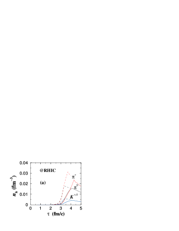
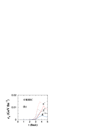
FIG. 2.: The time development of the hadron (a) number and (b) energy densities at RHIC. The solid (dashed) lines are for hadronization with (without) the barrier of color screening. The growth of the hadron densities is delayed in the former case and the maximum densities are lower.

Next we would like to lightly touch upon strangeness which is of great interest as it is one of the more promising signatures for the quark-gluon plasma. A great many number of papers have been written on the subject ever since it was first proposed in [33, 34]. One of the more interesting quantities is the strange to non-strange hadron ratio. It has been argued that the strangeness saturation parameter $\gamma_{s}$ determined from this ratio gives $\gamma_{s}\sim 0.5$ in p-p and $\gamma_{s}\sim 0.7$ according to [35] in A-A collisions. The latter is still under debate as refs. [36, 37] found that it was possible to fit AGS and SPS data with $\gamma_{s}=1$, while others such as refs. [35, 38] disagreed. A marked difference in $\gamma_{s}$ potentially suggests a quite different scenario in the collision core, one that may support a much more efficient production of strangeness. With our qualitative model, we do not attempt to make any statement about the definite value of $\gamma_{s}$ in A-A collisions. For that, one needs a good quantitative model. Here we merely make the observation that in our model, in which we do not include hadronic re-scattering, the strange to non-strange ratio progressively lowers down to the expected level from a rather high value to somewhere above 0.1 in Fig. 3. We attribute this to the progressive reduction of phase space for kaons since the probability of the formation of the more massive color singlet clusters with invariant mass $M>m_{\pi}+m_{K}$ is less as time progresses and the hadronization part of our model does not bias against the strange flavor. With and without color screening, there are some differences in this ratio which may not be so easy to see on the plot. The general behavior is the same in both cases, except in the case without color screening the curve ends up somewhat higher than the color screened one. The eventual strange to non-strange ratio therefore tends to be slightly lower when color screening is included simply because of phase space.

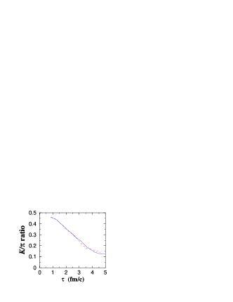
FIG. 3.: The strange to non-strange hadron ratio as a function of time with color screening (solid line) and without color screening (dashed line).

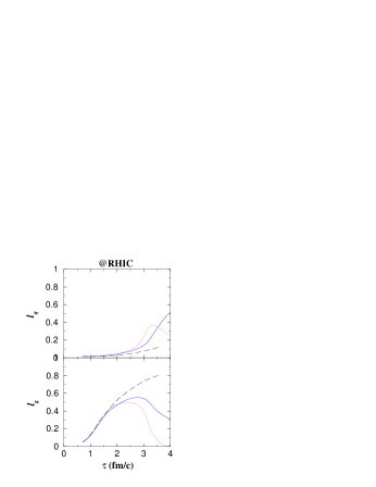
FIG. 4.: Chemical or parton equilibration here expressed in terms of the gluon and quark fugacities is seen to be disrupted by the hadronization independent of whether there is color screening (solid line) or there is no color screening (dotted line). The original case (long dashed line), where hadronization was not considered, is also shown for comparison.

We now turn to the effect of hadronization on the parton plasma. In Fig. 4, we plot the quark $l_{q}$ and gluon $l_{g}$ fugacities. Three cases are presented in the plot. The original time evolution of the parton plasma without hadronization are shown in long dashed lines. Then of the two cases with hadronization, dotted lines are for the case with no color screening and the solid lines are with color screening. The gluon fugacity $l_{g}$ which rose to above 0.8 in the original case is now affected quite significantly by the hadronization process. Instead of rising continuously, the two $l_{g}$ curves with hadronization now rise first, then stop ascending altogether before reversing to a downward descent. Remembering that we have included a term for non-perturbative gluon splitting which is prerequisite for hadronization into hadrons consisting only of quark and antiquark, this term is responsible for preventing $l_{g}$ from retracing the old ascending path. On the other hand, this same term is now enhancing the rise of $l_{q}$. We see that they are given a boost in the equilibration, rising at maximum to three or four times above the curve without hadronization. Confinement therefore interrupts the otherwise smooth time evolution of the partons. Comparing the two cases with hadronization, the one with color screening is again delayed as manifested already in the hadron density plots. At RHIC, it is highly unlikely that parton equilibration can be completed before the phase transition. By including hadronization, we show here that it is even more unlikely.

             

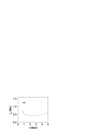
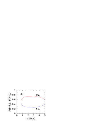
FIG. 5.: (a) The variation of the screening length $l_{D}$ during the time evolution ending in hadronization with (without) color screening is shown in solid (dashed) line. The two curves deviate from each other significantly at later times when hadronization is well underway. (b) The corresponding probabilities $P(b>l_{D}(\tau))$ and $P(b<l_{D}(\tau))$ as a function of time for the case with screening.

Lastly to argue for the importance of including both confinement and color screening, and to gain some insight into the internal struggle between the two, we show the variation of the screening length $l_{D}$ and the associated probabilities $P(b>l_{D})$, $P(b<l_{D})$ with $\tau$ in Fig. 5. At the time around $\tau=3$ fm, confinement has essentially been turned on. One can see that there is a huge difference in Fig. 5 (a) between the two cases of screening (solid line) and no screening (dashed line). In the latter, hadronization proceeded in an unhindered fashion therefore the parton medium essential for weakening the confining forces was quickly depleted. As a result the screening distance grew quickly. When the color screening barrier was erected against hadronization, the parton medium was able to hold itself together and maintained its screening power for much longer. In this latter case, the associated probabilities $P(b>l_{D})$ and $P(b<l_{D})$ are plotted in Fig. 5 (b). The much slower rise of $l_{D}$ meant that the probabilities also varied slowly although they had the expected behavior at larger times. We see trace of the one-loop behavior of the screening mass manifesting here too. Since it is rather time consuming to evolve the system on a computer so we stopped the time evolution once the qualitative features could be extracted. It is expected that eventually $P(b>l_{D})$ and $P(b<l_{D})$ will reach their correct limits at very large times. Relating Fig. 2 and Fig. 5, one might perhaps expect the value of the probability $P(b<l_{D})$ should be larger or equivalently $P(b>l_{D})$ smaller at the moment when the maximum densities in Fig. 2 occurred. This seemingly straight forward expectation is, however, not entirely justified because these maxima are results of a combination of factors: the actual sizes of the transition matrix elements, the switching factor $S(\alpha_{s})$ discussed in Sec. II B and the available parton densities. Confinement might be more favorable at later times but the number of available partons or the parton densities would be lower.

Finally, we would like to briefly discuss the problem with the transition matrix elements. We have already mentioned that there is no easy way to get readily usable expressions for these elements. Our chosen form is for convenience and it fulfills at least some aspects of the physical expectations. As to the constants, to obtain reasonable sensible results, there is a range of possible values. For the actual confinement matrix elements, we have actually chosen $\kappa_{0}=\kappa_{1}=\kappa_{1/2}$ for simplicity, since our main concern was the color screening effects and to point out that this aspect had been missing in the existing models. Using different values of these constants will change the actual numbers but the shape of the plots, the time sequence and therefore the qualitative picture that we tried to extract will remain intact.

REFERENCES

- [1] R.D. Field and S. Wolfram, Nucl. Phys. B 213, 65 (1983).
- [2] B.R. Webber, Nucl. Phys. B 238, 492 (1984).
- [3] K. Geiger, Phys. Rev. D 47, 133 (1993).
- [4] K. Geiger, Phys. Rev. D 46, 4965 (1992).
- [5] K. Geiger, Phys. Rev. D 46, 4986 (1992).
- [6] K. Geiger and J.I. Kapusta, Phys. Rev. Lett. 70, 1920 (1993).
- [7] J.I. Kapusta, Finite Temperature Field Theory, Cambridge University Press (1989).
- [8] L.P. Csernai and J.I. Kapusta, Phys. Rev. Lett. 69, 737 (1992).
- [9] L.P. Csernai and J.I. Kapusta, Phys. Rev. D 46, 1379 (1992).
- [10] L.P. Csernai, J.I. Kapusta, G.Y. Kluge, and E.E. Zabrodin, Z. Phys. C 58, 453 (1993).
- [11] S.M.H. Wong, Phys. Rev. C 56, 1075 (1997).
- [12] A.K. Rebhan, Phys. Rev. D 48, R3967 (1993).
- [13] K. Kajantie, M. Laine, J. Peisa, A. Rajantie, K. Rummukainen, and M. Shaposhnikov, Phys. Rev. Lett. 79, 3130 (1997).
- [14] K. Kajantie, M. Laine, J. Peisa, A. Rajantie, K. Rummukainen, and M. Shaposhnikov, Nucl. Phys. B 503, 357 (1997).
- [15] S.M.H. Wong, Nucl. Phys. A 607, 442 (1996).
- [16] S.M.H. Wong, Phys. Rev. C 54, 2588 (1996).
- [17] S.M.H. Wong, Nucl. Phys. A 638, 527c (1998).
- [18] S.M.H. Wong, Phys. Rev. C 58, 2358 (1998).
- [19] G. Baym, Phys. Lett. B 138, 18 (1984).
- [20] R.K. Ellis, W.J. Stirling and B.R. Webber, QCD and Collider Physics, Cambridge University Press (1996).
- [21] R.D. Field and R.P. Feynman, Phys. Rev. D 15, 2590 (1977).
- [22] R.D. Field and R.P. Feynman, Nucl. Phys. B 138, 1 (1978).
- [23] R. Hagedorn, Cargèse lectures in Physics, Vol. 6, Gordon and Breach (1973), eds. E. Schatzmann.
- [24] R. Hagedorn in Hot Hadronic Matter, NATO-ASI Series B 346, 13 (1995), Plenum Press, eds. J. Letessier, H. Gutbrod and J. Rafelski.
- [25] D. Amati and G. Veneziano, Phys. Lett. B 83, 87 (1979).
- [26] A. Bassetto, M. Ciafaloni and G. Marchesini, Phys. Lett. B 83, 207 (1979).
- [27] G. Marchesini, L. Trentadue and G. Veneziano, Nucl. Phys. B 181, 335 (1981).
- [28] T. Matsui and H. Satz, Phys. Lett. B 178, 416 (1986).
- [29] G. Grunberg, Phys. Lett. B 327, 121 (1996).
- [30] Yu.L. Dokshitzer, V.A. Khoze, and S.I. Troyan, Phys. Rev. D 53, 89 (1996).
- [31] D.V. Shirkov and I.L. Solovtsov, Phys. Rev. Lett. 79, 1209 (1997).
- [32] B.R. Webber, JHEP 10, 012 (1998).
- [33] B. Müller and J. Rafelski, Phys. Rev. Lett. 48, 1066 (1982).
- [34] T. Matsui, B. Svetitsky and L.D. McLerran, Phys. Rev. D 34, 783, 2047 (1986).
- [35] J. Sollfrank, F. Becattini, K. Redlich, and H. Satz, Nucl. Phys. A 638, 399c (1998).
- [36] P. Braun-Munzinger, J. Stachel, J.P. Wessels, and N. Xu, Phys. Lett. B 344, 43 (1995).
- [37] P. Braun-Munzinger, J. Stachel, J.P. Wessels, and N. Xu, Phys. Lett. B 365, 1 (1996).
- [38] J. Letessier and J. Rafelski, Acta. Phys. Pol. B 30, 153 (1999).