Dissipation, noise and DCC domain formation

Abstract

We investigate the effect of friction on domain formation in disoriented chiral condensate. We solve the equation of motion of the linear sigma model, in the Hartree approximation, including a friction and a white noise term. For quenched initial condition, we find that even in presence of noise and dissipation domain like structure emerges after a few fermi of evolution. Domain size as large as 5 fm can be formed.

25.75.+r, 12.38.Mh, 11.30.Rd

The possibility of forming disoriented chiral condensate (DCC) in relativistic heavy ion collisions has generated considerable research activities in recent years. The idea was first proposed by Rajagopal and Wilczek [2, 3, 4, 5]. They argued that for a second order chiral phase transition, the chiral condensate can become temporarily disoriented in the nonequilibrium conditions encountered in heavy ion collisions. As the temperature drops below $T_{c}$, the chiral symmetry begins to break by developing domains in which the chiral field is misaligned from its true vacuum value. The misaligned condensate has the same quark content and quantum numbers as do pions and essentially constitute a classical pion field. The system will finally relaxes to the true vacuum and in the process can emit coherent pions. Since the disoriented domains have well defined isospin orientation, the associated pions can exhibit novel centauro-like [6, 7, 8, 9] fluctuations of neutral and charged pions [10, 11, 12, 13].

Most dynamical studies of DCC have been based on the linear sigma model, in which the chiral degrees of freedom are described by the real O(4) field $\Phi=(\sigma,\roarrow{\Pi})$, having the equation of motion,

$$[\Box+\lambda(\Phi^{2}-v^{2})]\Phi=Hn_{\sigma}$$ (1)

The parameters of the model can be fixed by specifying the pion decay constant, $f_{\pi}$=92 MeV and the meson masses, $m_{\pi}$=135 MeV and $m_{\sigma}$=600 MeV, leading to $\lambda=(m_{\sigma}^{2}-m_{\pi}^{2})/2f_{\pi}^{2}$=20.14 and $v=[(m_{\sigma}^{2}-3m_{\pi}^{2})/(m_{\sigma}^{2}-m_{\pi}^{2})]^{1/2}f_{\pi}$=86.71 MeV and $H=(120.55MeV)^{3}$ [14]. It is apparent from eq.1 that the vacuum is aligned in the $\sigma$ direction $\Phi_{vac}=(f_{\pi},\bf{0})$ and at low temperature the fluctuations represent nearly free $\sigma$ and $\pi$ mesons. At very high temperature well above $v$, the field fluctuations are centered near zero and approximate O(4) symmetry prevails.

It is instructive to decompose the chiral field,

$$\Phi(r,t)=<\phi(r,t)>+\delta\phi(r,t)$$ (2)

where $<\phi>$is the mean field and $\delta\phi$ are the semiclassical fluctuations around $<\phi>$ and can be identified with quasi-particle excitations. Using eq.2 and taking the average of eq.1, the equation of motion for the mean fields in the Hartree approximation can be obtained as [14, 15],

$$\frac{\partial^{2}<\phi>}{\partial t^{2}}-\nabla^{2}<\phi>=\lambda(v^{2}-<\phi>^{2}-3<\delta\phi^{2}_{\|}>-<\delta\phi^{2}_{\bot}>)<\phi>+Hn_{\sigma}$$ (3)

where $<\phi>^{2}=<\phi_{i}><\phi_{i}>$, $\delta\phi_{\|}$ is the component of the fluctuation parallel to $<\phi>$ and $\delta\phi_{\bot}$ is the orthogonal component. This equation imply that the motion of the mean field is determined by the effective potential,

$$V(<\phi>)=\frac{\lambda}{4}(<\phi>^{2}+3<\delta\phi^{2}_{\|}>+<\delta\phi^{2}_{\bot}>-v^{2})$$ (4)

which clearly differs from the zero temperature one in presence of fluctuations. By varying the fluctuations, chiral symmetry can be restored or spontaneously broken. It is also evident that the evolution of the mean field critically depends on the initial values of the fluctuations. When $\delta^{2}\equiv(3<\delta\phi^{2}_{\|}>-<\delta\phi^{2}_{\bot}>)/6$ is large enough the chiral symmetry is approximately (as H$\neq$ 0) restored. If the explicit chiral symmetry breaking term is neglected, the phase transition takes place at the critical fluctuations $\delta^{2}_{c}\equiv v^{2}/6$. For $\delta^{2}<\delta^{2}_{c}$, the effective potential takes its minimum value at $<\phi>=(\sigma_{e},0)$, where $\sigma_{e}$ depends on $\delta^{2}$. When the mean fields are displaced from this equilibrium point to the central lump of the Mexican hat ($<\phi>\sim 0$), the effective mass square

$$m_{eff}^{2}=\lambda(v^{2}-<\phi>^{2}-3<\delta\phi^{2}_{\|}>-<\delta\phi^{2}_{\bot}>)$$ (5)

will become negative and DCC can form. Since the domain size is directly related to the time scale, during which the effective mass remains negative, it strongly depends on the initial condition of the system. By varying the $<\phi_{i}>$ and $\delta^{2}$, quench or annealing like initial condition can be obtained [15]. In an important paper Asakawa et al [15] studied eq.1 with initial condition corresponding to quench and annealing. They found that domains of disoriented chiral condensate with 4-5 fm in size can from through a quench. Annealing on the otherhand, leads to smaller sized domains.

In the present paper, our interest is to investigate the effect of friction on DCC domain formation. Dissipative effects like friction damp the motion of the fields, inhibiting large oscillations. Moreover, fluctuations-dissipations theorem require that dissipation be associated with noise. One would then expect large reduction in the DCC domain formation if friction is present in the system. This naive expectation was found to be true by Biro and Greiner [16]. Using the Langevin equation for the linear sigma model, they have investigated the interplay of friction and white noise on the evolution of the order parameter. While noise greatly diminishes the possibility of DCC domain formation, in some orbits, large instabilities can result, producing DCC domains. We have also studied the effect of friction on DCC domain formation using the Langevin equation [17]. There we found that for one-dimensional expansion on average large DCC domain can not be formed. However, in some particular orbit large instabilities can occur. This possibility also reduces with introduction of friction. However, if the friction is large, the system may be overdamped and then there is a possibility of DCC domain like formation. Present paper is an extension of the above study, the spatial part, which had been integrated out in our earlier analysis is being studied here.

Appropriate coordinates for heavy ion collisions are the proper time ($\tau$) and the rapidity (Y). The change can be effected by the following replacement,

$$\frac{\partial^{2}}{\partial t^{2}}-\frac{\partial^{2}}{\partial z^{2}}\rightarrow\frac{1}{\tau}\frac{\partial}{\partial\tau}\tau\frac{\partial}{\partial\tau}-\frac{1}{\tau^{2}}\frac{\partial^{2}}{\partial Y^{2}}$$ (6)

It can be seen from the above equation that with the introduction of proper time and rapidity, a dissipative term comes into effect in the equation of motion. To illustrate the role of friction, we further introduce a dissipative term ($\eta$) in the equation. However, fluctuations-dissipation theorem require that dissipation be associated with fluctuations. We thus include a white noise term also. To simplify our calculation, we assume boost-invariance in the system, Eq.3 can be written as,

$$\frac{\partial^{2}<\phi>}{\partial\tau^{2}}+(\frac{1}{\tau}+\eta)\frac{\partial<\phi>}{\partial\tau}= \frac{\partial^{2}<\phi>}{\partial x^{2}}+\frac{\partial^{2}<\phi>}{\partial y^{2}}+\lambda[v^{2}-<\phi>^{2}-T^{2}/2]<\phi>$$ (8)

$$+Hn_{\sigma}+\zeta(\tau,x,y)$$

where $\eta$ is the friction coefficient. $\zeta(\tau,x,y)$ is a Gaussian noise of temperature T with correlations,

$$<\zeta(\tau,x,y)>= 0$$ (10)

$$<\zeta_{a}(\tau_{1},x_{1},y_{1})\zeta_{b}(\tau_{2},x_{2},y_{2})>= 2\eta T\delta(\tau_{1}-\tau_{2})\delta(x_{1}-x_{2})\delta(y_{1}-y_{2})\delta_{ab}$$ (11)

It may also be noted that we have replaced the fluctuation term $3<\delta\phi^{2}_{\|}>-<\delta\phi^{2}_{\bot}>$ by its counterpart ($T^{2}/2$) in the finite temperature field theory [18, 19]. The equation of motion of fields then depend sensitively on the initial temperature of the system. In the following, we assume initial temperature to be $T_{c}=\sqrt{2f_{\pi}^{2}-2m_{\pi}^{2}/\lambda}$=123 MeV at the initial time $\tau_{i}$= 1 fm. The cooling of the system is described by the following equation appropriate for scaling expansion in 2-dimension,

$$\frac{\dot{T}}{T}+\frac{2}{3\tau}=0$$ (12)

The friction coefficient was assumed to be $\eta=\eta_{\pi}+\eta_{\sigma}$, where $\eta_{\pi,\sigma}$ are the friction coefficient of the pion and the sigma fields. They have been calculated by Rischke [20],

$$\eta_{\pi}= (\frac{4\lambda f_{\pi}}{N})^{2}\frac{m_{\sigma}^{2}}{4\pi m_{\pi}^{3}}\sqrt{1-\frac{4m_{\pi}^{2}}{m_{\sigma}^{2}}}\frac{1-exp(-m_{\pi}/T)}{1-exp(-m_{\sigma}^{2}/2m_{\pi}T)}\frac{1}{exp(m_{\sigma}^{2}-2m_{\pi}^{2})/2m_{p}iT)-1}$$ (14)

$$\eta_{\sigma}= (\frac{4\lambda f_{\pi}}{N})^{2}\frac{N-1}{8\pi m_{s}igma}\sqrt{1-\frac{4m_{\pi}^{2}}{m_{\sigma}^{2}}}\coth\frac{m_{\sigma}}{4T}$$ (15)

We solve the set of partial differential equations 8 with the quenched initial condition. Accordingly the initial fields are randomly distributed to a Gaussian form with the following parameters,

$$<\sigma>= (1-f(r))f_{\pi}$$ (17)

$$<\pi_{i}>= 0$$ (18)

$$<\sigma^{2}>-<\sigma>^{2}=<\pi_{i}^{2}>-<\pi_{i}>^{2}= v^{2}/4f(r)$$ (19)

$$<\dot{\sigma}>= <\dot{\pi_{i}}>=0$$ (20)

$$<\dot{\sigma}^{2}>=<\dot{\pi}>^{2}= v^{2}$$ (21)

The interpolation function

$$f(r)=[1+exp(r-r_{0})/\Gamma)]^{-1}$$ (22)

separates the central region where the initial field configuration is different from their vacuum expectation value. We use $r_{0}$=5 fm and $\Gamma$=0.5 fm.

The equation of motion was solved for 500 trajectories. For each trajectories, at each space-time we compute the effective mass $m^{2}_{eff}$. The phenomenon of long wavelength DCC amplification will occur whenever the effective mass squared is negative. To single out the trajectories for which maximum instabilities occur we calculate the following quantity,

$$G=\int|m_{eff}|\Theta(-m_{eff}^{2})\tau d\tau dxdy$$ (23)

This can be a measure of instability in a particular evolution. We call it amplification factor. This is an important parameter, as it directly relates to the size of DCC domains. In fig.1, we have shown the distribution of the amplification factor G for the 500 trajectories. The distribution is more or less Gaussian like. All the trajectories shows appreciable instability. The maximum and the minimum instabilities differing by $\sim$ 10%. Unlike 1-dimensional expansion, DCC domain formation is a distinct possibility in 2-dimensional expansion scenario. It is interesting to note that presence of friction and noise do not change the scenario to a great extent.

In fig.2, we show the contour plot of $\pi_{2}$ field for the most unstable orbit. Initially, at 1 fm, the field are randomly distributed. There is no domain like structure. After a few fermi of evolution, correlation starts to build up, and a domain like structure can be clearly seen. The domain like structure is most distinguished at 5 fm, where we see clear two domain formation. It may be noted that the two domains have different sign. The domain like structure persist at 7 fm also. The result is a clear indication of DCC like phenomena, even in presence of dissipation and noise.

In fig.3, we have shown the time evolution of the correlation function, defined as,

$$C(r,\tau)=\frac{\Sigma_{ij}\pi(i)\times\pi(j)}{\Sigma_{ij}|\pi(i)|\times|\pi(j)|}$$ (24)

where the sum is taken over those grid points $i$ and $j$ such that the distance between points is $r$. At 1 fm, there is no correlation beyond the lattice spacing (.25). A long range correlation emerges at 3 fm. The correlation length increases as the evolution time increases and at 5 fm it is as large as 5 fm, corroborating the pictorial result of fig.2

To summarize, we have investigated the effect of friction on the possible DCC domain formation. In the equation of motion for the linear sigma model fields, we include a friction and a white noise term and solve it assuming boost invariance. The noise term is required to be consistent with the fluctuation-dissipation theorem. Initial field configuration was assumed to be Gaussian random with quenched condition ($<\phi>=\dot{<\phi>}=0$). At each space-time $m^{2}_{eff}$ was calculated. Phenomenon of long wavelength amplification occurs when it becomes negative. For each trajectories, we calculate the amplification factor, as defined in eq.(). Amplification factor gives an indication of instability in the system. It was seen that for the 500 trajectories, the maximum and minimum instabilities do not differ much, indicating possibility of domain like structure formation in all the events. Clear domain like formation is seen in the event with maximum instability. For initial random field distribution, domain like structure emerges after a few fermi of evolution. Most distinct domain like structure is seen at 5 fm. There domain of 5 fm size is seen to be formed. We have also calculated the correlation function for the pion field. Similar result is also obtained there. Initially correlation donot extend beyond .25 fm, (the lattice spacing). After a few fm of evolution, long range correlation starts to build up. At 5 fm, correlation length of 5 fm is obtained. The result clearly indicate that the DCC domain formation is a distinct possibility, even in presence of friction and noise.

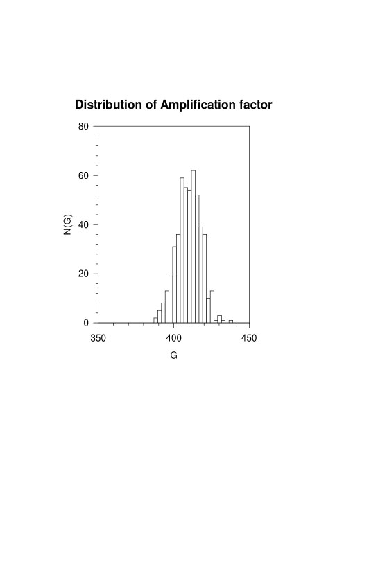
FIG. 1.: Distribution of the amplification factor G for the 500 trajectories calculated.

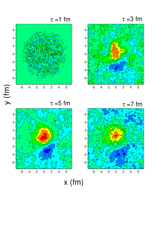
FIG. 2.: Contour plot of evolution of $\pi_{2}$ field for the event with maximum instability. At 5 fm, two domain like structure can be seen clearly. They have opposite sign.

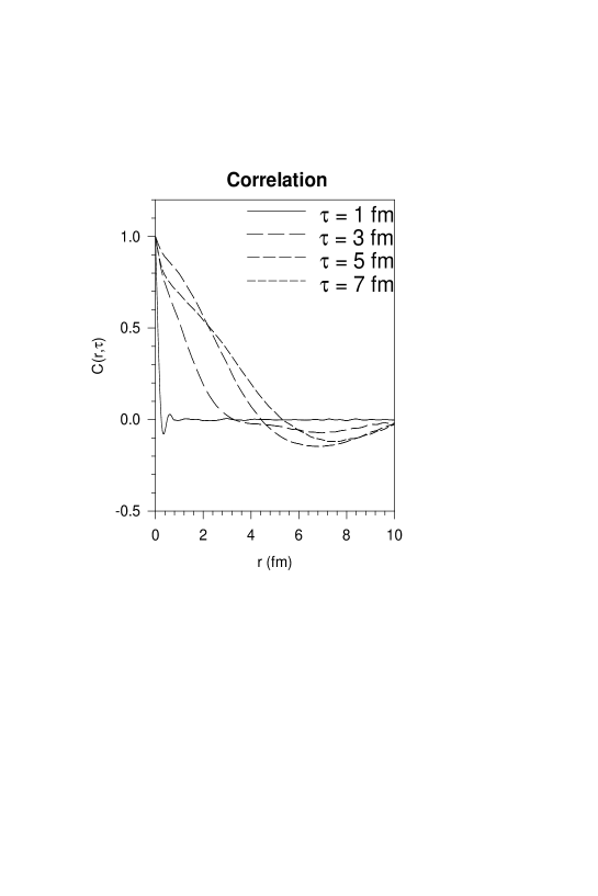
FIG. 3.: Evolution of the correlation function. Initially at 1 fm, there is no correlation beyond .25 fm, the lattice spacing. Large correlation devolop at later times.

REFERENCES

- [1] e-mail address:akc@veccal.ernet.in
- [2] K. Rajagopal and F. Wilczek, Nucl. Phys. B379, 395(1993).
- [3] K. Rajagopal and F. Wilczek,Nucl. Phys. B404, 577(1993).
- [4] K. Rajagopal,in Quark-Gluon Plasma 2, ed. R. Hwa, World Scientific (1995).
- [5] F. Wilczek, hep-ph/9308341. Phys. Reports 65,151(1980).
- [6] C. M. G. Lattes, Y. Fujimoto and S. Hasegawa, Phys. Reports, 154,247(1980).
- [7] G. Arnison et al, Phys. Lett. B 122,189 (1983).
- [8] G. J. Alner, Phys. Lett. B 180415,(1996); Phys. Reports 154,274 (1987).
- [9] J. R. Ren et al, Phys. Rev. D 38,1517 (1988).
- [10] A. A. Anselm and M. G. Ryskin , Phys. Lett. B 266,482 (1989).
- [11] A. A. Aneslm, Phys. Lett. B217, 169(1989).
- [12] J. D. Bjorken, K. L. Kowalski and C. C. Taylor , SLAC-PUB-6109 (1993), K.L. Kowalski K. L. and Taylor C. C., CWRUTH-92-6 (1992),hep-ph/9211282.
- [13] J. P. Blaizot ,A. Krzywicki , Phys. Rev.D46, 246 (1992).
- [14] J. Randrup, Report LBL-38125(1996), hep-ph/9602343.
- [15] M. Asakawa, Z. Huang and X.N. Wang, hep-ph/9408299.
- [16] T. S. Biro and C. Greiner, Phys. Rev. Lett. 79, 3138(1997).
- [17] A. K. Chaudhuri, nucl-th/9809018, Phys. Rev. D. (in press).
- [18] S. Gavin and B. Muller , Phys. Lett.B329,486 (1994).
- [19] J. Randrup, Phys. Rev. D 55,1188(1997).
- [20] D. H. Rischke, Phys. Rev. C, 2331 (1998)