Color Evaporation Induced Rapidity Gaps

Abstract

We show that soft color rearrangement of final states can account for the appearance of rapidity gaps between jets. In the color evaporation model the probability to form a gap is simply determined by the color multiplicity of the final state. This model has no free parameters and reproduces all data obtained by the ZEUS, H1, DØ, and CDF collaborations.

I Introduction

We show that the appearance of rapidity gaps between jets, observed at the HERA and Tevatron colliders, can be explained by supplementing the string model with the idea of color evaporation, or soft color. The inclusion of soft color interactions between the dynamical partons, which rearranges the string structure of the interaction, leads to a parameter-free calculation of the formation rate of rapidity gaps. The idea is extremely simple. Like in the string model, the dynamical partons are those producing the hard interactions, and the left-over spectators. A rapidity gap occurs whenever final state partons form color singlet clusters separated in rapidity. As the partons propagate within the hadronic medium, they exchange soft gluons which modify the string configuration. These large-distance fluctuations are probably complex enough for the occupation of different color states to approximately respect statistical counting. The probability to form a rapidity gap is then determined by the color multiplicity of the final states formed by the dynamical partons, and nothing else. All data obtained by ZEUS [1], H1 [2], DØ  [3], and CDF [4] collaborations are reproduced when this color structure of the interactions is superimposed on the usual perturbative QCD calculation for the production of the hard jets.

Rapidity gaps refer to intervals in pseudo-rapidity devoid of hadronic activity. The most simple example is the region between the final state protons, or its excited states, in $pp$ elastic scattering and diffractive dissociation. Such processes were first observed in the late 50’s in cosmic rays experiments [5] and have been extensively studied at accelerators [6]. Attempts to describe the formation of rapidity gaps have concentrated on Regge theory and the pomeron [7, 8], and on its possible QCD incarnation in the form of a colorless 2-gluon state [9, 10].

After the observation of rapidity gaps in deep inelastic scattering (DIS), it was suggested [11] that events with and without rapidity gaps are identical from a partonic point of view, except for soft color interactions that, occasionally, lead to a region devoid of color between final state partons. We pointed out [12] that this soft color mechanism is identical to the color evaporation mechanism [13] for computing the production rates of heavy quark pairs produced in color singlet onium states, like $J/\psi$. Moreover, we also suggested that the soft color model could provide a description for the production of rapidity gaps in hadronic collisions [12].

Color evaporation assumes that quarkonium formation is a two-step process: the pair of heavy quarks is formed at the perturbative level with scale $M_{Q}$, and bound into quarkonium at scale $\Lambda_{QCD}$ (see Fig. 1a). Heavy quark pairs of any color below open flavor threshold can form a colorless asymptotic quarkonium state provided they end up in a color singlet configuration after the inevitable exchange of soft gluons with the final state spectator hadronic system. The final color state of the quark pairs is not dictated by the hard QCD process, but by the fate of their color between the time of formation and emergence as an asymptotic state.

The success of the color evaporation model to explain the data on quarkonium production is unquestionable [14]. We show here that the straightforward application of the color evaporation approach to the string picture of QCD readily explains the formation of rapidity gaps between jets at the Tevatron and HERA colliders.

II Color Counting Rules

In the color evaporation scheme for calculating quarkonium production, it is assumed that all color configurations of the quark pair occur with equal probability. This must be a reasonable guess because, before formation as an asymptotic state, the heavy quark pair can exchange an infinite number of long wavelength soft gluons with the hadronic final state system in which it is immersed. For instance, the probability that a $Q\bar{Q}$ pair ends up in a color singlet state is $1/(1+8)$ because all states in $\bf 3\otimes\bf\bar{3}=\bf 8\oplus{\bf 1}$ are equally probable.

We propose that the same color counting applies to the final state partons in high $E_{T}$ jet production. In complete analogy with quarkonium, the production of high energy jets is a two-step process where a pair of high $E_{T}$ partons is perturbatively produced at a scale $E_{T}$, and hadronize into jets at a scale of order $\Lambda_{QCD}$ by stretching color strings between the partons and spectators. The strings subsequently hadronize. Rapidity gaps appear when a cluster of dynamical partons, i.e. interacting partons or spectators, form a color singlet (see Fig. 1b). As before, the probability for forming a color singlet cluster is inversely proportional to its color multiplicity.

In this scenario we expect that quark-quark processes possess a higher probability to form rapidity gaps than gluon-gluon reactions, because of their smaller color multiplicity. This simple idea is at variance with the two-gluon exchange model for producing gaps, in which $F_{QQ}<F_{GG}$, where $F_{QQ(GG)}$ is the gap probability of reactions initiated by quark-quark (gluon-gluon) collisions. We already confronted these diverging predictions using the Tevatron data [15]. We analyzed the gap fraction in $p\bar{p}$ collisions in terms of quark-quark, quark-gluon, and gluon-gluon subprocesses, i.e.

$$F_{gap}=\sum_{ij}F_{ij}d\sigma_{ij}/d\sigma\;\;,$$ (1)

where $i(j)$ is a quark or a gluon and $d\sigma=\sum_{ij}d\sigma_{ij}$. We found that $F_{QQ}>F_{GG}$. This somewhat unexpected feature of the data is in line with the soft color idea.

In order to better understand the soft color idea let us consider the formation of rapidity gaps between two jets in opposite hemispheres, which happens when the interacting parton forming the jet and the accompanying remnant system form a color singlet. This may occur for more than one subprocess $N$ and, therefore, the gap fraction is

$$F_{gap}=\frac{1}{d\sigma}~{}\sum_{N}F_{N}d\sigma_{N}\;\;,$$ (2)

where $F_{N}$ is the probability for gap formation in the $N^{th}$ subprocess, $d\sigma_{N}$ is the corresponding differential parton-parton cross section, and $d\sigma$ ($=\sum_{N}d\sigma_{N}$) is the total cross section. In our model, the probabilities $F_{N}$ are determined by the color multiplicity of the state and spatial distribution of partons while $d\sigma_{N}$ is evaluated using perturbative QCD.

The soft color procedure is obvious in a specific example: let us calculate the gap formation probability for the subprocesses

$\displaystyle p\;\bar{p}\;\to Q^{V}\bar{Q}^{V}\to Q\,\bar{Q}\,X\,Y\;\;,$where $Q^{V}$ stands for $u$ or $d$ valence quark, and $X$ $(Y)$ is the diquark remnant of the proton (antiproton). The final state is composed of the $X$ ($\bf 3\otimes\bf 3$) color spectator system with rapidity $\eta_{X}=+\infty$, the $Y$ ($\bf\bar{3}\otimes\bf{\bar{3}}$) color spectator system with $\eta_{Y}=-\infty$, one $\bf 3$ parton $j_{1}$, and one $\bf{\bar{3}}$ parton $j_{2}$. It is the basic assumption of the soft color scheme that by the time these systems hadronize, any color state is equally likely. One can form a color singlet final state between $X$ and $j_{1}$ since ${\bf 3\otimes 3\otimes 3}={\bf 10\oplus 8\oplus 8\oplus 1}$, with probability $1/27$. Because of overall color conservation, once the system $X\otimes j_{1}$ is in a color singlet, so is the system $Y\otimes j_{2}$. On the other hand, it is not possible to form a color singlet system with $j_{1}$ and $Y$. Moreover, to form a rapidity gap these systems ($j_{1}\otimes X$ and $j_{2}\otimes Y$) must not overlap in rapidity space. Since the experimental data consists of events where the two jets are in opposite hemispheres, the only additional requirements are $j_{1}$ to be in the same hemisphere as $X$, i.e. $\eta_{1}>0$, and $j_{2}$ to be in the opposite hemisphere ($\eta_{1}\cdot\eta_{2}<0$). In this configuration, the color strings linking the remnant and the parton in the same hemisphere will not hadronize in the region between the two jets. We have thus produced two jets separated by a rapidity gap using the color counting rules which form the basis of the color evaporation scheme for calculating quarkonium production.

As it is clear from the above example, the application of the soft color model for rapidity gap formation requires the analyses of the color multiplicity of the possible partonic subprocesses. In the next sections, we apply this model to the production of rapidity gaps between jets in photoproduction at HERA and hadronic collisions at the Tevatron, spelling out the relevant counting rules.

III Rapidity Gaps at HERA

The parton diagram for dijet photoproduction is shown in Fig. 2a. It is related to the $ep$ cross section by

$$\sigma_{ep\rightarrow j_{1}j_{2}XY}(s)=\int_{y_{min}}^{y_{max}}\int_{Q^{2}_{min}}^{Q^{2}_{max}}F_{e}^{\gamma}(y,Q^{2})\,\sigma_{p\gamma\rightarrow j_{1}j_{2}XY}(W)\,dy\,dQ^{2}\;\;,$$ (3)

where $W$ is the center-of-mass energy of the $p\gamma$ system, $y=W^{2}/s$ is the fraction of the electron momentum carried by the photon, and $Q^{2}$ is the photon virtuality. $Q^{2}$ ranges from $Q^{2}_{min}=M_{e}^{2}y^{2}/(1-y)$ to $Q^{2}_{max}$ which depends on the kinematic coverage of the experimental apparatus. The distribution function of photons in the electron is

$$F_{e}^{\gamma}(y,Q^{2})=\frac{\alpha}{2\pi y\,Q^{2}}\left[1+(1-y)^{2}-\frac{2M_{e}^{2}y^{2}}{Q^{2}}\right]\;\;,$$ (4)

where $M_{e}$ is the electron mass and $\alpha$ is the fine-structure constant.

The $p\gamma$ cross section is related to the parton-parton cross section by

$$\sigma_{p\gamma\rightarrow j_{1}j_{2}XY}(W)=\sum_{a,b}\int\!\!\int F_{p}^{a}(x_{a})\,F_{\gamma}^{b}(x_{b})\,\sigma_{ab\to p_{1}p_{2}}(\hat{s})\,dx_{a}\,dx_{b}\;\;,$$ (5)

where $F_{p}^{a}(x_{a})$ ($F_{\gamma}^{b}(x_{b})$) is the distribution function for parton $a$ ($b$) in the proton (photon) and $\sqrt{\hat{s}}=\sqrt{x_{a}x_{b}}\,W$ is the parton-parton center-of-mass energy. For direct $p\gamma$ reactions ($b\equiv\gamma$), $F_{\gamma}^{\gamma}(x_{b})=\delta(1-x_{b})$. The hadronic system $X$ $(Y)$ is the proton (photon) remnant, and $j_{1(2)}$ is the jet which is initiated by the parton $p_{1(2)}$. The proton is assumed to travel in the positive rapidity direction, and the $t$-channel momentum squared is defined as $t=(P_{a}-P_{1})^{2}$, where $P_{a}$ is the momentum of the parton $a$, and $P_{1}$ is the momentum of the parton $p_{1}$. The expressions for the parton-parton invariant amplitudes can be found, for instance, in reference [16].

We present in Table I the irreducible decomposition of active parton systems that yield color singlet states, e. g. ${\bf 3\otimes 8=15\oplus 6\oplus 3}$ is omitted. Taking into account this table, it is simple to obtain the $SU(3)_{color}$ representations and the gap formation probability for all possible subprocesses. These are displayed in Table II. Notice that only resolved photon processes can produce rapidity gaps because there is no hadronic remnant associated with direct photons.

One of the features of the color configurations shown in Table II is that, for all classes of subprocesses, when a color singlet is (not) allowed in one of the clusters, the same happens for the other one. Moreover, it can happen that the color multiplicities are different in the two clusters. In this case the probability for gap formation is given by the largest of the two probabilities because, once that cluster forms a color singlet, the other cluster must do so as well by overall color conservation.

A ZEUS Results

The ZEUS collaboration [1] has measured the formation of rapidity gaps between jets produced in $ep$ collisions with $0.2<y<0.85$ and photon virtuality $Q^{2}<4$ GeV². Jets were defined by a cone radius of 1.0 in the $(\eta,\phi)$ plane, where $\eta$ is the pseudorapidity and $\phi$ is the azimuthal angle. In the event selection, jets were required to have $E_{T}>6$ GeV, to not overlap in rapidity ($\Delta\eta=|\eta_{1}-\eta_{2}|>2$), to have a mean position $|\bar{\eta}|<0.75$, and to be in the region $\eta<2.5$. The cross sections were measured in $\Delta\eta$ bins in the range $2\leq\Delta\eta\leq 4$.

For the above event selection, we evaluated the dijet differential cross section $d\sigma^{jets}/d\Delta\eta$, which is the sum of the direct ($d\sigma_{dir}$) and the resolved photon ($d\sigma_{res}$) cross sections. We used the GRV-LO [17] distribution function for the proton, and the GRV [18] for the photon. We fixed the renormalization and factorization scales at $\mu_{R}=\mu_{F}=E_{T}/2$, and calculated the strong coupling constant for four active flavors with $\Lambda_{QCD}=350$ MeV. Our results are confronted with the experimental data in Fig. 3a, showing that we describe well both the shape and absolute normalization of the total dijet cross section. Notice that the bulk of the cross section originates from resolved events.

Now we turn to dijet events showing a rapidity gap. We evaluate the differential cross section $d\sigma^{gap}/d\Delta\eta$ which has two sources of gap events: color evaporation gaps ($d\sigma^{gap}_{cem}$) and background gaps ($d\sigma^{gap}_{bg}$). In our model, the gap cross section is the weighted sum over resolved events

$$d\sigma^{gap}_{cem}=\sum_{N}F_{N}~{}d\sigma^{N}_{res}\;\;,$$ (6)

with the gap probability $F_{N}$ for the different processes given in Table II. Background gaps are formed when the region of rapidity between the jets is devoid of hadrons because of statistical fluctuation of ordinary soft particle production. Their rate should fall exponentially as the rapidity separation $\Delta\eta$ between the jets increases [1]. We parametrize the background gap probability as

$$F_{bg}(\Delta\eta)=e^{b(2-\Delta\eta)}\;\;,$$ (7)

where $b$ is a constant. The background gap cross section is then written as

$$d\sigma_{bg}^{gap}=F_{bg}(\Delta\eta)~{}(d\sigma^{jets}-d\sigma^{gap}_{cem})\;\;.$$ (8)

Notice that the jet definition used by ZEUS implies that the gap cross section must be equal to the total dijet cross section at $\Delta\eta=2$. This parametrization of the background does take this fact into account. Moreover, background gaps can be formed in both resolved and direct processes.

Our results are compared with the experimental data in Fig. 3b, where we fitted $b=2.9$ and used the same QCD parameters of Fig. 3a. This value of $b$ agrees with $b=2.7\pm 0.3$ found by ZEUS collaboration, when they approximated the non-background gap fraction by a constant. As we can see from this figure, the color evaporation model describes very well the gap formation between jets at HERA. It is noteworthy that for large values of $\Delta\eta$ the contribution of the background gap is negligible. In this region the data is correctly predicted by the color evaporation mechanism alone, with the probability of gap formation uniquely determined by statistical counting of color states.

The gap frequency $F^{gap}(\Delta\eta)=d\sigma^{gap}/d\sigma^{jets}$ is shown in Fig. 4a, where we show the contributions of the color evaporation mechanism and the background. Within the color evaporation framework we can easily predict other differential distributions for the gap events, which can be used to further test our model. As an example, we present in Fig. 4b the gap frequency predicted by the color evaporation model as a function of the jet transverse energy for large rapidity separations ($\Delta\eta>3$), assuming that the background has been subtracted. There is currently no data on this distribution.

B H1 Results

We also performed an identical analysis for the data obtained by the H1 collaboration [2]. They used the same cone size for the jet definition $(\Delta R=1)$, and collected events produced in proton-photon reactions with center-of-mass energy in the range $158<W<247$ GeV and with photon virtuality $Q^{2}<0.01$ GeV². They also imposed cuts on the jets: $-2.82<\eta<2.35$ and $E_{T}>4.5$ GeV. Our results are compared with the preliminary experimental data on Fig. 5a where we used $b=2.3$ to describe the background in the H1 kinematic range. As before, color evaporation induces gap formation with a rate compatible with observation. We show in Fig. 5b our predictions for the background subtracted gap frequency as a function of the jet transverse energy for large rapidity separations $\Delta\eta>3$.

C Survival Probability at HERA

Our computation of gap rates using color evaporation is free of parameters and therefore predicts absolute rates, as well as their dependence on kinematic variables. In practice, this prediction is diffused by the necessity to introduce a gap survival probability $S_{p}$, which accounts for the fact that genuine gap events, as predicted by the theory, can escape experimental identification because additional partonic interactions in the same event produce secondaries which spoil the gap. Its value has been estimated for high energy $p\bar{p}$ interactions to be of order a few tens of percent. The fact that the color evaporation calculation correctly accommodates the absolute gap rate observed in $p\gamma$ collisions implies that $S_{p}=1$. There is a simple explanation for this value. The dijet cross section is dominated by resolved photons. However, for resolved processes, a secondary partonic interaction which could fill the gap is unlikely because it requires resolving the photon in 2 partons. Although this routinely happens at high energies for hadrons, it does not for photons.

IV Rapidity Gaps at Tevatron

The kinematics for dijet production in $p\bar{p}$ collisions is illustrated in Fig. 2b, where we denoted by $X$ ($Y$) the proton (antiproton) remnant, and $j_{1(2)}$ is a parton giving rise to a jet. The proton is assumed to travel in the positive rapidity direction. The dijet production cross section is related to the parton-parton one via

$$\sigma_{p\bar{p}\rightarrow j_{1}j_{2}XY}(s)=\sum_{a,b}\int\!\!\int F_{p}^{a}(x_{a})\,F_{\bar{p}}^{b}(x_{b})\,\sigma_{ab\to p_{1}p_{2}}(\hat{s})\,dx_{a}\,dx_{b}\;\;,$$ (9)

where $s$ ($\hat{s}=x_{a}x_{b}s$) is the (subprocess) center-of-mass energy squared and $F^{a(b)}_{p(\bar{p})}$ is the distribution function for the parton $a$ $(b)$. We evaluated the dijet cross sections using MRS-J distribution functions [19] with renormalization and factorization scales $\mu_{R}=\mu_{F}=\sqrt{\hat{s}}$.

The color evaporation model prediction for the gap production rates in $p\bar{p}$ collisions is analogous to the one in $p\gamma$ interactions, with the obvious replacement of the photon by the antiproton, represented as a ${\bf\bar{3}\otimes\bar{3}\otimes\bar{3}}$ system. The color subprocesses and their respective gap formation probabilities are listed in Table III.

Both experimental collaborations presented their data with the background subtracted. The CDF collaboration measured the appearance of rapidity gaps at two different $p\bar{p}$ center-of-mass energies. For the data taken at $\sqrt{s}=1800$ GeV, they required that both jets to have $E_{T}>20$ GeV, and to be produced in opposite sides ($\eta_{1}\cdot\eta_{2}<0$) within the region $1.8<|\eta|<3.5$. For the lower energy data, $\sqrt{s}=630$ GeV, they required both jets to have $E_{T}>8$ GeV, and to be produced in opposite sides within the region $|\eta|>1.8$. Since the experimental distributions are normalized to unity, on average, we do not need to introduce an ad-hoc gap survival probability. Therefore, our predictions do not exhibit any free parameter to be adjusted, leading to a important test of the color evaporation mechanism.

In Figs. 6, 7, and 8 we compare our predictions with the experimental observations of the gap fraction as a function of the jets transverse energy, their separation in rapidity, and the Bjorken-$x$ of the colliding partons, respectively. As we can see, the overall performance of the color evaporation model is good since it describes correctly the shape of almost all distributions. This is an impressive result since the model has no free parameters to be adjusted.

The DØ collaboration has made similar observations at $\sqrt{s}=1800$ GeV. They required that both jets to have $E_{T}>15$ GeV, to be produced in opposite sides ($\eta_{1}\cdot\eta_{2}<0$) within the region $1.9<|\eta|<4.1$, and to be separated by $|\Delta\eta|>4.0$. In Fig. 9 our results are compared with experimental observations of the dependence of the gap frequency on jet transverse energy, where we used a gap survival probability $S_{p}=30\%$ to reproduce the absolute normalization. This is consistent with qualitative theoretical estimates; see discussion below. As we can see, the fraction of gap events increases with the transverse energy of the jets. This is expected once the dominant process for the rapidity gap formation is quark-quark fusion, which becomes more important at larger $E_{T}$. Apart from the lowest transverse energy bin, data and theory are in good agreement. In Fig. 10 we compare our prediction for the dependence of the gap frequency with the separation between the jets. Agreement is satisfactory although the absolute value of our predictions for low transverse energy is somewhat higher than data as shown in Fig. 9. Finally, in Fig. 11 we show our results for the mean value of the Bjorken-$x$ of the events, where all correlations between the jet transverse energy and rapidity have been included. Again, the agreement between theory and data is satisfactory except for the low transverse energy bins.

A Survival Probability at Tevatron

We estimated the survival probability of rapidity gaps formed at $p\bar{p}$ collisions, comparing our predictions with the values of gap fraction actually observed. Assuming that the survival probability varies only with the collision center-of-mass energy, and not with the jet’s transverse energy, we evaluated the average survival probability

$$S_{p}=\frac{F^{gap}_{exp}}{F^{gap}_{cem}}\;\;.$$ (10)

In order to extract $\bar{S}_{p}$ we combined the DØ and CDF available data at each center-of-mass energy: 630 and 1800 GeV. We found $\bar{S}_{p}(1800)=34.4\pm 3.3$% and $\bar{S}_{p}(630)=65.4\pm 12$%, a value compatible with the calculation of Ref. [20] based on the Regge model, which yields $S_{p}(1800)=32.6$%. For individual contributions and further details see Table IV. Moreover, we have that $\bar{S}_{p}(630)/\bar{S}_{p}(1800)=1.9\pm 0.4$, which is compatible with the theoretical expectation $2.2\pm 0.2$ obtained in Ref. [21].

Using the extracted values of the survival probability, we contrasted the color evaporation model predictions for the gap fraction corrected by $\bar{S}_{p}$ ($F^{gap}_{cor}=F^{gap}_{cem}\times\bar{S}_{p}$) with the experimental data in Table IV. We can also compare the ratio $R=F^{gap}_{cor}(630)/F^{gap}_{cor}(1800)$ with the experimental result. DØ has measured this fraction for jets with $E_{T}>12$ GeV for both energies, and they found $R=3.4\pm 1.2$; we predict $R=2.5\pm 0.5$. On the other hand, CDF measured this ratio using different values for $E_{T}^{min}$ at 630 GeV and 1800 GeV; they obtained $R=2.0\pm 0.9$ while we obtained $R=2.0\pm 0.4$ for the same kinematical arrangement.

V Conclusion

In summary, the occurrence of rapidity gaps between hard jets can be understood by simply applying the soft color, or color evaporation, scheme for calculating quarkonium production, to the conventional perturbative QCD calculation of the production of hard jets. The agreement between data and this model is impressive.

Final state color multiplicity	Color singlet fraction
${\bf 3}\otimes{\bf\bar{3}}={\bf 8}\oplus{\bf 1}$	1/9
${\bf 3}\otimes{\bf 3}\otimes{\bf 3}={\bf 10}\oplus 2({\bf 8})\oplus{\bf 1}$	1/27
${\bf 3}\otimes{\bf\bar{3}}\otimes{\bf 8}={\bf 27}\oplus 2({\bf 10})\oplus 3({\bf 8})\oplus{\bf 1}$	1/72
${\bf 3}\otimes{\bf 3}\otimes{\bf 3}\otimes{\bf 8}={\bf 35}\oplus 3({\bf 27})\oplus 5({\bf 10})\oplus 6({\bf 8})\oplus 2({\bf 1})$	2/216
${\bf 3}\otimes{\bf 3}\otimes{\bf 3}\otimes{\bf 3}\otimes{\bf\bar{3}}={\bf 35}\oplus 3({\bf 27})\oplus 6({\bf 10})\oplus 8({\bf 8})\oplus 3({\bf 1})$	3/243

TABLE I.: Irreducible decomposition of relevant $SU(3)$ representations. Only those that generate singlets are shown.

Subprocess	$j_{1}$	$j_{2}$	$X$	$Y$	$F_{N}$
$Q^{V}Q\rightarrow QQ$	${\bf 3}$	${\bf 3}$	${\bf 3\otimes 3}$	${\bf\bar{3}}$	$1/9\;\forall\;\eta_{1}$
$Q^{S}Q\rightarrow QQ$	${\bf 3}$	${\bf 3}$	${\bf 3\otimes 3\otimes 3\otimes\bar{3}}$	${\bf\bar{3}}$	$1/9\;\forall\;\eta_{1}$
$\bar{Q}^{S}\bar{Q}\rightarrow\bar{Q}\bar{Q}$	${\bf\bar{3}}$	${\bf\bar{3}}$	${\bf 3\otimes 3\otimes 3\otimes 3}$	${\bf 3}$	$1/9\;\forall\;\eta_{1}$
$Q^{V}\bar{Q}\rightarrow Q\bar{Q}$	${\bf 3}$	${\bf\bar{3}}$	${\bf 3\otimes 3}$	${\bf 3}$	$1/9$ for $\eta_{1}>\eta_{2}$
$Q^{S}\bar{Q}\rightarrow Q\bar{Q}$	${\bf 3}$	${\bf\bar{3}}$	${\bf 3\otimes 3\otimes 3\otimes\bar{3}}$	${\bf 3}$	$1/9$ for $\eta_{1}>\eta_{2}$
$\bar{Q}^{S}Q\rightarrow\bar{Q}Q$	${\bf\bar{3}}$	${\bf 3}$	${\bf 3\otimes 3\otimes 3\otimes 3}$	${\bf\bar{3}}$	$1/9$ for $\eta_{1}>\eta_{2}$
$Q^{V}\bar{Q}\rightarrow GG$	${\bf 8}$	${\bf 8}$	${\bf 3\otimes 3}$	${\bf 3}$	$0$
$Q^{S}\bar{Q}\rightarrow GG$	${\bf 8}$	${\bf 8}$	${\bf 3\otimes 3\otimes 3\otimes\bar{3}}$	${\bf 3}$	$0$
$\bar{Q}^{S}Q\rightarrow GG$	${\bf 8}$	${\bf 8}$	${\bf 3\otimes 3\otimes 3\otimes 3}$	${\bf\bar{3}}$	$0$
$Q^{V}G\rightarrow QG$	${\bf 3}$	${\bf 8}$	${\bf 3\otimes 3}$	${\bf 3\otimes\bar{3}}$	$1/27$ for $\eta_{1}>\eta_{2}$
$Q^{S}G\rightarrow QG$	${\bf 3}$	${\bf 8}$	${\bf 3\otimes 3\otimes 3\otimes\bar{3}}$	${\bf 3\otimes\bar{3}}$	$1/72$ for $\eta_{1}>\eta_{2}$
$\bar{Q}^{S}G\rightarrow\bar{Q}G$	${\bf\bar{3}}$	${\bf 8}$	${\bf 3\otimes 3\otimes 3\otimes 3}$	${\bf 3\otimes\bar{3}}$	$1/72$ for $\eta_{1}>\eta_{2}$
$GQ\rightarrow GQ$	${\bf 8}$	${\bf 3}$	${\bf 3\otimes 3\otimes 3}$	${\bf\bar{3}}$	$1/9$ for $\eta_{1}>\eta_{2}$
$G\bar{Q}\rightarrow G\bar{Q}$	${\bf 8}$	${\bf\bar{3}}$	${\bf 3\otimes 3\otimes 3}$	${\bf 3}$	$1/9$ for $\eta_{1}>\eta_{2}$
$GG\rightarrow Q\bar{Q}$	${\bf 3}$	${\bf\bar{3}}$	${\bf 3\otimes 3\otimes 3}$	${\bf 3\otimes\bar{3}}$	$0$
$GG\rightarrow GG$	${\bf 8}$	${\bf 8}$	${\bf 3\otimes 3\otimes 3}$	${\bf 3\otimes\bar{3}}$	$1/72\;\forall\;\eta_{1}$

TABLE II.: Color multiplicities and gap probabilities $F_{N}$ for the reaction $p\,\gamma\to j_{1}\,j_{2}\,X\,Y$, where $X$ and $Y$ are respectively the proton and the photon remnant systems. $Q^{V(S)}$ stands for valence (sea) quarks, and we assumed that the proton travels in the positive rapidity direction.

Subprocess	$j_{1}$	$j_{2}$	$X$	$Y$	$F_{N}$
$Q^{V}Q^{S}\rightarrow QQ$	${\bf 3}$	${\bf 3}$	${\bf 3\otimes 3}$	${\bf\bar{3}\otimes\bar{3}\otimes\bar{3}\otimes\bar{3}}$	$1/27\;\forall\;\eta_{1}$
$Q^{S}Q^{S}\rightarrow QQ$	${\bf 3}$	${\bf 3}$	${\bf 3\otimes 3\otimes 3\otimes\bar{3}}$	${\bf\bar{3}\otimes\bar{3}\otimes\bar{3}\otimes\bar{3}}$	$1/81\;\forall\;\eta_{1}$
$\bar{Q}^{S}\bar{Q}^{V}\rightarrow\bar{Q}\bar{Q}$	${\bf\bar{3}}$	${\bf\bar{3}}$	${\bf 3\otimes 3\otimes 3\otimes 3}$	${\bf\bar{3}\otimes\bar{3}}$	$1/27\;\forall\;\eta_{1}$
$\bar{Q}^{S}\bar{Q}^{S}\rightarrow\bar{Q}\bar{Q}$	${\bf\bar{3}}$	${\bf\bar{3}}$	${\bf 3\otimes 3\otimes 3\otimes 3}$	${\bf\bar{3}\otimes\bar{3}\otimes\bar{3}\otimes 3}$	$1/81\;\forall\;\eta_{1}$
$Q^{V}\bar{Q}^{V}\rightarrow Q\bar{Q}$	${\bf 3}$	${\bf\bar{3}}$	${\bf 3\otimes 3}$	${\bf\bar{3}\otimes\bar{3}}$	$1/27$ for $\eta_{1}>0$
$Q^{V}\bar{Q}^{S}\rightarrow Q\bar{Q}$	${\bf 3}$	${\bf\bar{3}}$	${\bf 3\otimes 3}$	${\bf\bar{3}\otimes\bar{3}\otimes\bar{3}\otimes 3}$	$1/27$ for $\eta_{1}>0$
$Q^{S}\bar{Q}^{V}\rightarrow Q\bar{Q}$	${\bf 3}$	${\bf\bar{3}}$	${\bf 3\otimes 3\otimes 3\otimes\bar{3}}$	${\bf\bar{3}\otimes\bar{3}}$	$1/27$ for $\eta_{1}>0$
$Q^{S}\bar{Q}^{S}\rightarrow Q\bar{Q}$	${\bf 3}$	${\bf\bar{3}}$	${\bf 3\otimes 3\otimes 3\otimes\bar{3}}$	${\bf\bar{3}\otimes\bar{3}\otimes\bar{3}\otimes 3}$	$1/81$ for $\eta_{1}>0$
$\bar{Q}^{S}Q^{S}\rightarrow\bar{Q}Q$	${\bf\bar{3}}$	${\bf 3}$	${\bf 3\otimes 3\otimes 3\otimes 3}$	${\bf\bar{3}\otimes\bar{3}\otimes\bar{3}\otimes\bar{3}}$	$1/81$ for $\eta_{1}>0$
$Q^{V}\bar{Q}^{V}\rightarrow GG$	${\bf 8}$	${\bf 8}$	${\bf 3\otimes 3}$	${\bf\bar{3}\otimes\bar{3}}$	$0$
$Q^{V}\bar{Q}^{S}\rightarrow GG$	${\bf 8}$	${\bf 8}$	${\bf 3\otimes 3}$	${\bf\bar{3}\otimes\bar{3}\otimes\bar{3}\otimes 3}$	$0$
$Q^{S}\bar{Q}^{V}\rightarrow GG$	${\bf 8}$	${\bf 8}$	${\bf 3\otimes 3\otimes 3\otimes\bar{3}}$	${\bf\bar{3}\otimes\bar{3}}$	$0$
$Q^{S}\bar{Q}^{S}\rightarrow GG$	${\bf 8}$	${\bf 8}$	${\bf 3\otimes 3\otimes 3\otimes\bar{3}}$	${\bf\bar{3}\otimes\bar{3}\otimes\bar{3}\otimes 3}$	$0$
$\bar{Q}^{S}Q^{S}\rightarrow GG$	${\bf 8}$	${\bf 8}$	${\bf 3\otimes 3\otimes 3\otimes 3}$	${\bf\bar{3}\otimes\bar{3}\otimes\bar{3}\otimes\bar{3}}$	$0$
$Q^{V}G\rightarrow QG$	${\bf 3}$	${\bf 8}$	${\bf 3\otimes 3}$	${\bf\bar{3}\otimes\bar{3}\otimes\bar{3}}$	$1/27$ for $\eta_{1}>0$
$Q^{S}G\rightarrow QG$	${\bf 3}$	${\bf 8}$	${\bf 3\otimes 3\otimes 3\otimes\bar{3}}$	${\bf\bar{3}\otimes\bar{3}\otimes\bar{3}}$	$1/108$ for $\eta_{1}>0$
$\bar{Q}^{S}G\rightarrow\bar{Q}G$	${\bf\bar{3}}$	${\bf 8}$	${\bf 3\otimes 3\otimes 3\otimes 3}$	${\bf\bar{3}\otimes\bar{3}\otimes\bar{3}}$	$1/108$ for $\eta_{1}>0$
$G\bar{Q}^{V}\rightarrow G\bar{Q}$	${\bf 8}$	${\bf\bar{3}}$	${\bf 3\otimes 3\otimes 3}$	${\bf\bar{3}\otimes\bar{3}}$	$1/27$ for $\eta_{1}>0$
$G\bar{Q}^{S}\rightarrow G\bar{Q}$	${\bf 8}$	${\bf\bar{3}}$	${\bf 3\otimes 3\otimes 3}$	${\bf\bar{3}\otimes\bar{3}\otimes\bar{3}\otimes 3}$	$1/108$ for $\eta_{1}>0$
$GQ^{S}\rightarrow GQ$	${\bf 8}$	${\bf 3}$	${\bf 3\otimes 3\otimes 3}$	${\bf\bar{3}\otimes\bar{3}\otimes\bar{3}\otimes\bar{3}}$	$1/108$ for $\eta_{1}>0$
$GG\rightarrow Q\bar{Q}$	${\bf 3}$	${\bf\bar{3}}$	${\bf 3\otimes 3\otimes 3}$	${\bf\bar{3}\otimes\bar{3}\otimes\bar{3}}$	$0$
$GG\rightarrow GG$	${\bf 8}$	${\bf 8}$	${\bf 3\otimes 3\otimes 3}$	${\bf\bar{3}\otimes\bar{3}\otimes\bar{3}}$	$1/108\;\forall\;\eta_{1}$

TABLE III.: Color multiplicities and gap probabilities $F_{N}$ for the reaction $p\,\bar{p}\to j_{1}\,j_{2}\,X\,Y$, where $X$ and $Y$ are respectively the proton and the antiproton remnant systems. $Q^{V(S)}$ stands for valence (sea) quarks, and we assumed that the proton travels in the positive rapidity direction.

$\sqrt{s}$ (GeV)	$E_{T}^{min}$ (GeV)	$F^{gap}_{cem}$ (%)	$F^{gap}_{exp}$ (%)	$S_{p}$ (%)	$F^{gap}_{cem}\times\bar{S}_{p}$ (%)
1800	30	2.91	$0.94\pm 0.13$ (DØ)	$32.3\pm 4.5$	$1.00\pm 0.10$
1800	20	2.49	$1.13\pm 0.16$ (CDF)	$45.4\pm 6.4$	$0.85\pm 0.08$
1800	12	2.24	$0.54\pm 0.17$ (DØ)	$24.1\pm 7.6$	$0.77\pm 0.07$
630	12	2.97	$1.85\pm 0.38$ (DØ)	$62.3\pm 12.8$	$1.94\pm 0.36$
630	8	2.55	$2.3\pm 1.0$ (CDF)	$90.2\pm 39.2$	$1.67\pm 0.31$

TABLE IV.: Gap frequencies and survival probabilities. The average survival probabilities are $\bar{S}_{p}(1800)=34.4\pm 3.3$%, and $\bar{S}_{p}(630)=65.4\pm 12.1$%. Theoretical uncertainties are not included.

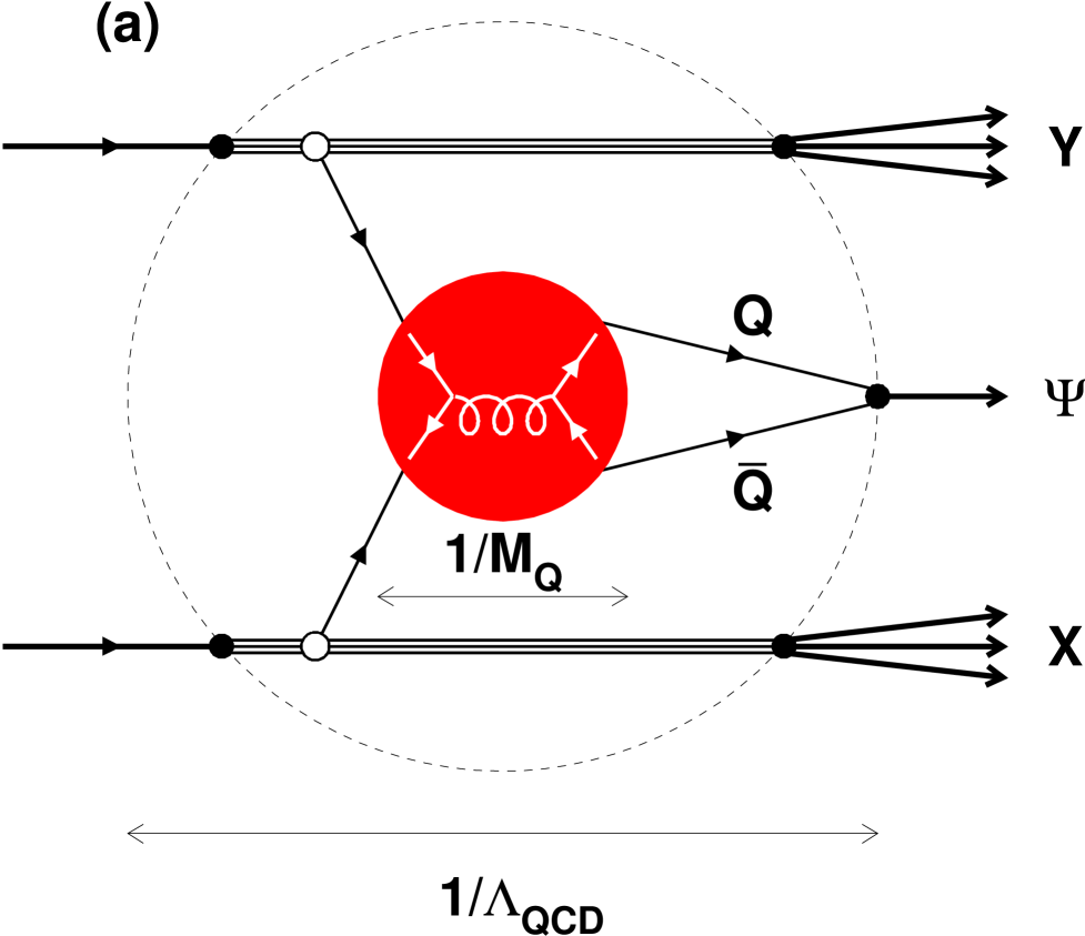
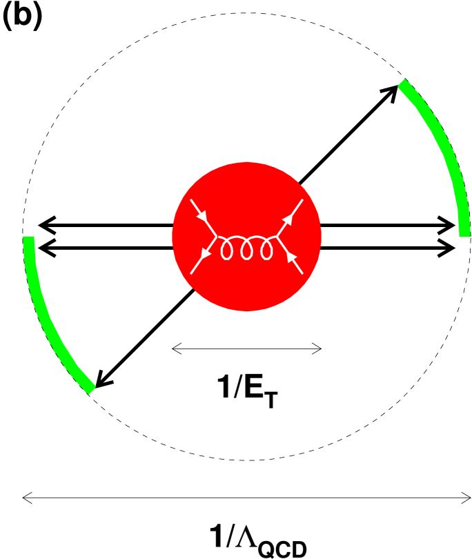
FIG. 1.: Sketch of the soft color mechanism for (a) quarkonium production; (b) rapidity gap formation. We indicate in the figures the typical scale of the hard scattering and the hadronization scale $1/\Lambda_{QCD}$. The soft color rearrangement occurs between these two distinct scales.

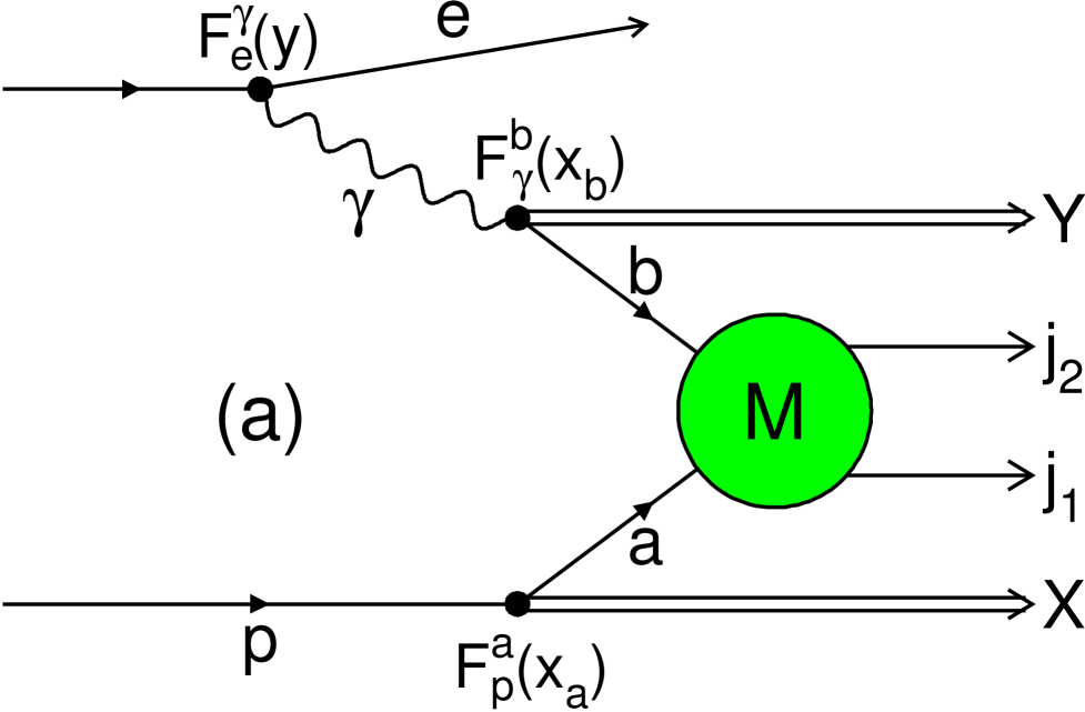
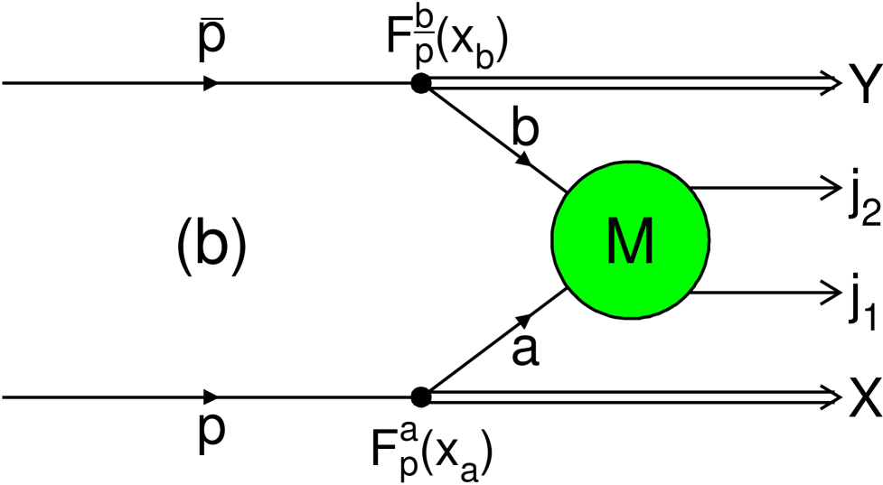
FIG. 2.: Kinematics for dijet photoproduction (a) and hadroproduction (b). The proton and its remnants system $X$ move in the positive rapidity direction.

FIG. 3.: Differential dijet cross section as function of the rapidity between the jets: (a) all events; (b) events presenting a rapidity gap. The points with error bars represent the data obtained by the ZEUS collaboration [1].

FIG. 4.: Fraction of rapidity gap events as a function of: (a) the gap size $\Delta\eta$; (b) the jet transverse energy $E_{T}$ at large rapidity separations ($\Delta\eta>3$). We imposed the cuts used by the ZEUS collaboration.

FIG. 5.: Same as in Fig. 4 for the H1 experiment.

  

FIG. 6.: Dependence of the gap frequency on the jet transverse energy as measured by the CDF collaboration. The absolute normalization is arbitrary.

  

FIG. 7.: The same as Fig. 6 for half the gap size.

  

FIG. 8.: The same as Fig. 6 for the Bjorken-$x$ of each jet. Two entries per event are included in the distribution.

  

FIG. 9.: Gap fraction as a function of the jet $E_{T}$ as measured by the DØ collaboration at $\sqrt{s}=1800$ GeV. We used a gap survival probability of $30\%$ to obtain the normalization shown.

  

FIG. 10.: Gap fraction as a function of the jets rapidity separation for two different values of the jets transverse energy. The survival probability is the same as in Fig. 9.

  

FIG. 11.: Gap fraction as a function of the average Bjorken-$x$ of the two jets for events collected in different rapidity intervals and jet transverse energy bins. The survival probability is the same as in Fig. 9.