TUM-HEP-353/99
ZU-TH 19/99
LNF-99/021(P)
OUTP–99–38P
August 1999

Connections between $\varepsilon^{\prime}/\varepsilon$ and

Rare Kaon Decays in Supersymmetry

A.J. Buras¹, G. Colangelo², G. Isidori³,

A. Romanino⁴ and L. Silvestrini¹

¹⁾ Technische Universität München, Physik Department
D-85747 Garching, Germany
²⁾ Institut für Theoretische Physik der Universität Zürich,
Winterthurerstr. 190, CH–8057 Zürich–Irchel, Switzerland
³⁾ INFN, Laboratori Nazionali di Frascati
P.O. Box 13, I–00044 Frascati, Italy
⁴⁾ Department of Physics, Theoretical Physics, University of Oxford,
Oxford OX1 3NP, UK

Abstract

We analyze the rare kaon decays $K_{L}\to\pi^{0}\nu\bar{\nu}$, $K^{+}\to\pi^{+}\nu\bar{\nu}$, $K_{L}\to\pi^{0}e^{+}e^{-}$ and $K_{L}\to\mu^{+}\mu^{-}$ in conjunction with the CP violating ratio $\varepsilon^{\prime}/\varepsilon$ in a general class of supersymmetric models in which $Z$- and magnetic-penguin contributions can be substantially larger than in the Standard Model. We point out that radiative effects relate the double left-right mass insertion to the single left-left one, and that the phenomenological constraints on the latter reflect into a stringent bound on the supersymmetric contribution to the $Z$ penguin. Using this bound, and those coming from recent data on $\varepsilon^{\prime}/\varepsilon$, we find ${\rm BR}(K_{L}\to\pi^{0}\nu\bar{\nu})\stackrel{{\scriptstyle<}}{{{}_{\sim}}}1.2\cdot 10^{-10}$, ${\rm BR}(K^{+}\to\pi^{+}\nu\bar{\nu})\stackrel{{\scriptstyle<}}{{{}_{\sim}}}1.7\cdot 10^{-10}$, ${\rm BR}(K_{L}\to\pi^{0}e^{+}e^{-})_{\rm dir}\stackrel{{\scriptstyle<}}{{{}_{\sim}}}2.0\cdot 10^{-11}$, assuming the usual determination of the CKM parameters and neglecting the possibility of cancellations among different supersymmetric effects in $\varepsilon^{\prime}/\varepsilon$. Larger values are possible, in principle, but rather unlikely. We stress the importance of a measurement of these three branching ratios, together with improved data and improved theory of $\varepsilon^{\prime}/\varepsilon$, in order to shed light on the realization of various supersymmetric scenarios. We reemphasize that the most natural enhancement of $\varepsilon^{\prime}/\varepsilon$, within supersymmetric models, comes from chromomagnetic penguins and show that in this case sizable enhancements of $BR(K_{L}\to\pi^{0}e^{+}e^{-})_{\rm dir}$ can also be expected.

1 Introduction

Flavour-Changing Neutral Current (FCNC) processes provide a powerful tool for testing the Standard Model and the physics beyond it. Of particular interest are the rare kaon decays $K_{L}\to\pi^{0}\nu\bar{\nu}$, $K^{+}\to\pi^{+}\nu\bar{\nu}$ and $K_{L}\to\pi^{0}e^{+}e^{-}$ which are governed by $Z$-penguin diagrams. The latter diagrams play also a substantial role in the CP violating ratio $\varepsilon^{\prime}/\varepsilon$. The most recent experimental results for this ratio,

$$\mathop{\mbox{Re}}(\varepsilon^{\prime}/\varepsilon)=\left\{\begin{array}[]{ll}(28.0\pm 4.1)\cdot 10^{-4}&{\rm(KTeV)\ \cite[cite]{[\@@bibref{}{KTEV}{}{}]}}\\ (18.5\pm 7.3)\cdot 10^{-4}&{\rm(NA48)\ \cite[cite]{[\@@bibref{}{NA48}{}{}]}}\end{array}\right.$$ (1)

are in the ball park of the earlier result of the NA31 collaboration at CERN, $(23.0\pm 6.5)\cdot 10^{-4}$ [3], and substantially higher than the value of E731 at Fermilab, $(7.4\pm 5.9)\cdot 10^{-4}$ [4]. The grand average (according to the PDG recipe) including NA31, E731, KTeV and NA48 results, reads

$$\mathop{\mbox{Re}}(\varepsilon^{\prime}/\varepsilon)=(21.2\pm 4.6)\cdot 10^{-4}~{},$$ (2)

very close to the NA31 result but with a smaller error. The error should be further reduced once complete data from both collaborations will be analyzed. It is also of great interest to see what value for $\varepsilon^{\prime}/\varepsilon$ will be measured by KLOE at Frascati, which uses a different experimental technique than KTeV and NA48.

The estimates of $\varepsilon^{\prime}/\varepsilon$ within the Standard Model (SM) are generally below the data but in view of large theoretical uncertainties stemming from hadronic matrix elements one cannot firmly conclude that the data on $\varepsilon^{\prime}/\varepsilon$ imply new physics [5, 6, 7, 8, 9]. On the other hand the apparent discrepancy between the SM estimates and the data invites for speculations about non-standard contributions to $\varepsilon^{\prime}/\varepsilon$. Indeed the KTeV result prompted several recent analyses of $\varepsilon^{\prime}/\varepsilon$ within various extensions of the Standard Model (see e.g. [10]) and particularly within supersymmetry [11, 12]. Unfortunately these extensions have many parameters and if only $\varepsilon^{\prime}/\varepsilon$ is considered the analyses are not very conclusive.

The approach we want to pursue in the present paper is different: we will adopt a model-independent point of view within a generic supersymmetric extension of the Standard Model with minimal particle content, and study what are the implications of a supersymmetric $\varepsilon^{\prime}/\varepsilon$ for the rare decays. To do so we will use the mass-insertion approximation [13]. Despite the presence of a large number of parameters within this framework, only a few of them are allowed to contribute substantially to $\varepsilon^{\prime}/\varepsilon$. Phenomenological constraints, coming mainly from $\Delta S=2$ transitions [14], make the contribution of most of them to $\Delta S=1$ amplitudes very small compared to the Standard Model one. The only parameters which survive are the left-right mass insertions contributing to the Wilson coefficients of $Z$- and magnetic-penguin operators. As we will discuss below, the reason for this simplification is a dimensional one: these are the only two classes of operators of dimension less than six contributing to $\varepsilon^{\prime}/\varepsilon$. Supposing that the enhancement of the Wilson coefficients of either of these two (or both) type of operators is responsible for the observed value of $\varepsilon^{\prime}/\varepsilon$, a corresponding effect in the rare decays should be observed. In what follows we will analyze in detail the relations between the size of the effect in $\varepsilon^{\prime}/\varepsilon$ and those in the rare decays.

The same kind of logic was already followed by two of us in [15]. There, this kind of analysis was carried through under the assumption that the dominant effect in $\Delta S=1$ transitions was only an enhanced $\bar{s}dZ$ vertex. This analysis was motivated by an observation of another two of us [16] that the branching ratios of rare kaon decays could be considerably enhanced, in a generic supersymmetric model, by large contributions to the effective $\bar{s}dZ$ vertex due to a double left-right mass insertion. This double mass insertion had not been included in earlier analyses of rare kaon decays in supersymmetry [17, 18]. In the latter papers only single mass insertions were taken into account, leading to modest enhancements of rare-decay branching ratios, up to factors 2-3 at most, as opposed to the possible enhancement of more than one order of magnitude allowed by the double mass insertion [16]. The conclusion of the analysis in [15] was that the data on $\varepsilon^{\prime}/\varepsilon$ may constrain considerably the double left-right mass insertion and the corresponding enhancement of the rare-decays branching ratios.

In the present paper we will improve the analysis in [15] with the aim to answer the following questions:

• Can the large double mass insertions suggested in [16] be further constrained? As we will see this is indeed the case.

• What is the impact of these new constraints on the analysis in [15]?

• What is the impact on this analysis of contributions from chromomagnetic and $\gamma$-magnetic penguins to $\varepsilon^{\prime}/\varepsilon$ and $K_{L}\to\pi^{0}e^{+}e^{-}$ respectively?

As we mentioned above, in generic supersymmetric theories a sizable contribution to $\varepsilon^{\prime}/\varepsilon$ could also be generated by the chromomagnetic-dipole operator. Actually, within supersymmetric models with approximate flavor symmetries, the latter mechanism seems to be more natural than a strong enhancement of the $\bar{s}dZ$ vertex [11]. Interestingly, if the Wilson coefficient of the chromomagnetic-dipole operator gets enhanced, one should also expect a sizable effect in the branching ratio of $K_{L}\to\pi^{0}e^{+}e^{-}$, due to the $\gamma$-magnetic penguin. In fact their Wilson coefficients receive contributions from the same type of mass insertion.

The paper is organized as follows: In Section 2 we identify the dominant SUSY contributions to $|\Delta S|=1$ amplitudes as those of dimension less than six. In Section 3 we summarize the effective Hamiltonian for $|\Delta S|=1$ transitions concentrating on the operators of dimension four (effective $\bar{s}dZ$ vertex) and five (magnetic penguins) and their corresponding Wilson coefficients. Here we introduce three effective couplings which characterize the supersymmetric contributions to the Wilson coefficients of these operators: $\Lambda_{t}$ for the $Z$ penguin and $\Lambda_{g}^{\pm}$ for the magnetic ones. In Section 4 we collect the basic formulae for $\varepsilon^{\prime}/\varepsilon$ and rare kaon decays in terms of these effective couplings. In particular we calculate the magnetic contributions to $\varepsilon^{\prime}/\varepsilon$ and $K_{L}\to\pi^{0}e^{+}e^{-}$. In Section 5 we analyze indirect bounds on the effective couplings. The main result of this section is an improved upper bound on $|\Lambda_{t}|$ coming from renormalization group considerations. In Section 6 we present a detailed numerical analysis of rare kaon decays taking into account the recent data on $\varepsilon^{\prime}/\varepsilon$, the present information on the short distance contribution to ${\rm BR}(K_{L}\to\mu^{+}\mu^{-})$ and the bounds on effective couplings derived in Section 5. Analyzing various scenarios we calculate upper limits on ${\rm BR}(K_{L}\to\pi^{0}e^{+}e^{-})_{\rm dir}$, ${\rm BR}(K_{L}\to\pi^{0}\nu\bar{\nu})$ and ${\rm BR}(K^{+}\to\pi^{+}\nu\bar{\nu})$. We present a summary and our conclusions in Section 7.

2 SUSY contributions to $|\Delta S|=1$ amplitudes

In the Standard Model FCNC amplitudes are generated only at the quantum level. The same remains true also in low-energy supersymmetric models with unbroken $R$ parity, minimal particle content and generic flavour couplings. The flavour structure of a generic SUSY model is quite complicated and a convenient way to parametrize the various flavour-mixing terms is provided by the so-called mass-insertion approximation [13]. This consists in choosing a simple basis for the gauge interactions and, in that basis, to perform a perturbative expansion of the squark mass matrices around their diagonal. In the following we will employ a squark basis where all quark-squark-gaugino vertices involving down-type quarks are flavor diagonal.

In the case of $|\Delta S|=1$ transitions we can distinguish between two large classes of one-loop diagrams:

• Box diagrams. These are present both in $|\Delta S|=1$ and $|\Delta S|=2$ amplitudes. In both cases the integration of the heavy degrees of freedom, associated with the superpartners, necessarily leads to effective four-quark operators of dimension six. The Wilson coefficients of these operators are therefore suppressed by two powers of a supersymmetry-breaking scale, that we generically denote by $M_{S}$. Here $1/M_{S}^{2}$ plays a role similar to $1/M^{2}_{W}$ in the SM case.

  Since any mass-insertion carries at most $|\Delta S|=1$, the leading contribution to $|\Delta S|=2$ transitions starts at second order in this expansion. Denoting by $\delta$ the generic ratio of off-diagonal terms over diagonal ones in the squark mass matrices, the coupling of $|\Delta S|=2$ effective operators turns out to be of ${\cal O}(\delta^{2}/M_{S}^{2})$. This has to be compared with the dominant SM coupling that is of ${\cal O}(\lambda_{t}^{2}/M_{W}^{2})$, where $\lambda_{t}=V^{*}_{ts}V_{td}$. If we then impose that the supersymmetric contribution to $|\Delta S|=2$ amplitudes is at most of the order of the SM one, we find

  $$\delta/M_{S}\stackrel{{\scriptstyle<}}{{{}_{\sim}}}\lambda_{t}/M_{W}~{}.$$ (3)

  In the case of $|\Delta S|=1$ amplitudes, the leading supersymmetric contribution starts already at first order in $\delta$, similarly to the SM one that is linear in $\lambda_{t}$. However, the dimensional suppression factor is always $1/M_{S}^{2}$ in the SUSY case and $1/M_{W}^{2}$ in the SM one. Therefore, if $M_{S}\gg M_{W}$, the constraint (3) implies that the supersymmetric contribution to $|\Delta S|=1$ box diagrams is suppressed with respect to the SM one. This naive argument is confirmed by the detailed analysis of [14], where it has been shown that $|\Delta S|=2$ constraints always dominate over $|\Delta S|=1$ ones, as long as we consider only dimension-six operators generated by box diagrams with gluino exchange.

• Penguin diagrams. At the one-loop level this kind of diagrams is present only in $|\Delta S|=1$ amplitudes. Effective operators with lowest dimension generated by photon and gluon penguins are the so-called “magnetic” operators of dimension five. The coupling of these operators is of ${\cal O}(\delta/M_{S})$ and therefore potentially competing with the SM contributions even if we impose the bound (3). This naive conclusion is again confirmed by detailed analyses of gluino mediated amplitudes [14]. In this context it is found that only the chromomagnetic operator, induced by ${\tilde{d}}_{L(R)}-{\tilde{s}}_{R(L)}$ mixing, could lead to sizable $(\stackrel{{\scriptstyle>}}{{{}_{\sim}}}10^{-3})$ contributions to $\varepsilon^{\prime}/\varepsilon$ without violating any constraints from $\varepsilon$.

  A different situation occurs in the case of $Z$-penguin diagrams, where the breaking of $SU(2)_{L}$ allows to build an effective dimension-four operator of the type $s_{L}\gamma^{\mu}d_{L}Z_{\mu}$. Denoting by $C_{Z}$ the dimensionless coupling of this operator, the integration of the heavy $Z$ field leads to an effective four-fermion operator proportional to $C_{Z}/M_{Z}^{2}$ without any explicit $1/M_{S}$ suppression. This potential enhancement is partially compensated by the fact that the leading contribution to $C_{Z}$ arises only at second order in the mass-insertion [16]. However, the absence of any $1/M_{S}$ suppression makes this term particularly interesting both for rare decays [16] and $\varepsilon^{\prime}/\varepsilon$ [15].

Given the above considerations, in the following we will restrict our attention only to the dominant SUSY effects in $|\Delta S|=1$ amplitudes: those generated by the “magnetic” dimension-five operators, induced by gluino exchange, and those generated by the $\bar{s}dZ$ vertex mediated by chargino exchange. Interestingly, under this assumption only the off-diagonal left-right entries of squark mass matrices are involved, in particular the ${\tilde{d}}_{L(R)}-{\tilde{s}}_{R(L)}$ mixing for the magnetic operators and the ${\tilde{u}}^{(s,d)}_{L}-{\tilde{t}}_{R}$ one for the $\bar{s}dZ$ vertex.

What we will not consider are the gluino and the chargino contributions to irreducible dimension-six operators. The former have been explicitly calculated in [14] and found to be negligible, the latter are suppressed by ${\cal O}(M^{2}_{W}/M^{2}_{S})$ with respect to the corresponding contributions mediated by the $\bar{s}dZ$ vertex. To control the accuracy of our approximation, we have explicitly checked that the impact of these terms is below $10\%$, with respect to the dominant ones, for squark/gaugino masses above $\sim 300$ GeV. Finally, we will completely ignore the neutralino contributions which are known to be negligible due to the smallness of both electroweak and down-type Yukawa couplings [18].

Since a large $\bar{s}dZ$ vertex is already present in the SM, the corresponding SUSY corrections can be easily incorporated without modifying the structure of the SM $|\Delta S|=1$ effective Hamiltonian. On the other hand, the dimension-five operators, neglected within the SM, require an adequate treatment and will be discussed in detail below.

3 Effective Hamiltonian

3.1 Operators and Wilson Coefficients

On the basis of the discussion in the previous section, we introduce here the effective Hamiltonian containing all the relevant operators of dimension smaller than six. The only dimension-four operator of interest is the one given by the $\bar{s}dZ$ vertex:

$${\cal H}^{d=4}_{\rm eff}=-\frac{G_{F}}{\sqrt{2}}\frac{e}{\pi^{2}}M_{Z}^{2}\frac{\cos\Theta_{W}}{\sin\Theta_{W}}Z_{ds}\bar{s}_{L}\gamma_{\mu}Z^{\mu}d_{L}\,+\,{\rm h.c.}~{},$$ (4)

where

$$Z_{ds}=\lambda_{t}C_{0}(x_{t})+\tilde{\lambda}_{t}H_{0}(x_{q\chi})~{}.$$ (5)

Here the first term on the r.h.s is the Standard Model contribution (evaluated in the ’t Hooft-Feynman gauge) and the second one represents the dominant supersymmetric effect. The couplings $\lambda_{t}$ and $\tilde{\lambda}_{t}$ are defined by

$$\lambda_{t}=V_{ts}^{*}V_{td}~{},\qquad{\tilde{\lambda}}_{t}=(\delta^{U}_{LR})_{23}(\delta^{U}_{LR})_{13}^{*}~{},$$ (6)

where $V_{ij}$ are the elements in the CKM matrix and, denoting by $M^{2}_{[U,D]}$ the squark mass matrices,

$$\left(\delta^{[U,D]}_{AB}\right)_{ij}=\left(M^{2}_{[U,D]}\right)_{i_{A}j_{B}}\left/\langle M^{2}_{[U,D]}\rangle\right.~{}.$$ (7)

Explicit expressions for the functions $C_{0}$ and $H_{0}$ will be given below.

The magnetic operators of dimension five appear in the effective Hamiltonian in the following way:

$${\cal H}_{\rm eff}^{d=5}=(C^{+}_{\gamma}Q^{+}_{\gamma}+C^{-}_{\gamma}Q^{-}_{\gamma}+C^{+}_{g}Q^{+}_{g}+C^{-}_{g}Q^{-}_{g})+{\rm h.c.}~{},$$ (8)

where we have chosen the following operator basis:

$$Q^{\pm}_{\gamma} = \frac{Q_{d}e}{16\pi^{2}}\left({\bar{s}}_{L}\sigma^{\mu\nu}F_{\mu\nu}d_{R}\pm{\bar{s}}_{R}\sigma^{\mu\nu}F_{\mu\nu}d_{L}\right)~{},$$ (9)

$$Q^{\pm}_{g} = \frac{g}{16\pi^{2}}\left({\bar{s}}_{L}\sigma^{\mu\nu}t^{a}G^{a}_{\mu\nu}d_{R}\pm{\bar{s}}_{R}\sigma^{\mu\nu}t^{a}G^{a}_{\mu\nu}d_{L}\right)~{},$$ (10)

Full expressions for the Wilson coefficients generated by gluino exchange at the SUSY scale can be found in [14]. We are interested here only in the contributions proportional to $1/m_{\tilde{g}}$, which are given by

$$C^{\pm}_{\gamma}(m_{\tilde{g}}) = \frac{\pi\alpha_{s}(m_{\tilde{g}})}{m_{\tilde{g}}}\left[\left(\delta^{D}_{LR}\right)_{21}\pm\left(\delta^{D}_{LR}\right)^{*}_{12}\right]F_{0}(x_{gq})\;\;,$$ (11)

$$C^{\pm}_{g}(m_{\tilde{g}}) = \frac{\pi\alpha_{s}(m_{\tilde{g}})}{m_{\tilde{g}}}\left[\left(\delta^{D}_{LR}\right)_{21}\pm\left(\delta^{D}_{LR}\right)^{*}_{12}\right]G_{0}(x_{gq})\;\;,$$ (12)

where the $\delta_{ij}$ are defined in (7) and the functions $F_{0}$ and $G_{0}$ are given in (20) and (21).

In the $(Q^{\pm}_{g},Q^{\pm}_{\gamma})$ basis, the leading order anomalous dimension matrix reads

$$\gamma=\left(\begin{array}[]{cc}8/3&0\\ &\\ 32/3&4/3\end{array}\right)~{}.$$ (13)

Therefore, integrating out SUSY particles at the scale $m_{\tilde{g}}>m_{t}$, one has

$$C^{\pm}_{\gamma}(m_{c}) = \eta^{2}\left[C^{\pm}_{\gamma}(m_{\tilde{g}})+8\,(1-\eta^{-1})\,C^{\pm}_{g}(m_{\tilde{g}})\right],$$ (14)

$$C^{\pm}_{g}(m_{c}) = \eta\,C^{\pm}_{g}(m_{\tilde{g}}),$$ (15)

where

$$\eta=\left(\frac{\alpha_{s}(m_{\tilde{g}})}{\alpha_{s}(m_{t})}\right)^{\frac{2}{21}}\left(\frac{\alpha_{s}(m_{t})}{\alpha_{s}(m_{b})}\right)^{\frac{2}{23}}\left(\frac{\alpha_{s}(m_{b})}{\alpha_{s}(m_{c})}\right)^{\frac{2}{25}}~{}.$$ (16)

The dimension-five operators in (8) in principle mix also with $Q_{2}$, the leading dimension-six operator of the SM $|\Delta S|=1$ effective Hamiltonian (see e.g. [19]). However, the effect of this mixing can be neglected as long as we are interested in large enhancements of the Wilson coefficients of the dimension-five operators with respect to the SM case (more than one order of magnitude in the imaginary parts, as suggested in [11]). Therefore, as first approximation, in the following we will neglect the mixing of $Q_{g(\gamma)}^{\pm}$ with $Q_{2}$.

3.2 Basic Functions

The basic functions relevant for our analysis are

$$B_{0}(x)={1\over 4}\left[{x\over{1-x}}+{{x\ln(x)}\over{(x-1)^{2}}}\right]~{},$$ (17)

$$C_{0}(x)={x\over 8}\left[{{x-6}\over{x-1}}+{{3x+2}\over{(x-1)^{2}}}\;\ln(x)\right]~{},$$ (18)

$$H_{0}(x)=-\frac{x(x^{3}-6x^{2}+3x+2+6x\ln(x))}{48(1-x)^{4}}~{},$$ (19)

$$F_{0}(x) = {{4x(1+4\,x-5\,{x^{2}}+4\,x\,\ln(x)+2\,{x^{2}}\,\ln(x))}\over{3\,{{\left(1-x\right)}^{4}}}}~{},$$ (20)

$$G_{0}(x) = \frac{x(22-20x-2x^{2}+16x\ln(x)-x^{2}\ln(x)+9\ln(x))}{3(1-x)^{4}}~{},$$ (21)

with the corresponding mass ratios

$$x_{t}=m_{t}^{2}/m_{W}^{2}~{},\qquad x_{q\chi}=m_{{\tilde{q}}}^{2}/m_{\tilde{\chi}}^{2}~{},\qquad x_{gq}=m_{{\tilde{g}}}^{2}/m_{\tilde{q}}^{2}~{}.$$ (22)

$B_{0}(x_{t})$ and $C_{0}(x_{t})$ are the box and $Z^{0}$ penguin diagram functions in the Standard Model respectively. The function $H_{0}(x_{q\chi})$ appears in the SUSY contribution to the $\bar{s}dZ$ vertex [16]. The functions $F_{0}(x_{gq})$ and $G_{0}(x_{gq})$ enter the contributions of $\gamma$-magnetic and chromomagnetic penguin operators respectively [14].

3.3 Effective couplings

The SUSY Wilson coefficients which we have given above depend explicitly on the sparticle masses via the functions $H_{0}$, $F_{0}$ and $G_{0}$. The dependence is not very strong, as can be seen from Fig. 1, where we plot the three functions normalized to their values at $x=1$ $(H_{0}(1)=-1/96,\ F_{0}(1)=2/9,\ G_{0}(1)=-5/18)$. On the other hand the relations between $\varepsilon^{\prime}/\varepsilon$ and the rare decays which we want to investigate here, are almost independent from the spectra of the SUSY particles. In fact these relations are most conveniently described in terms of three effective couplings defined as follows:

$$\Lambda_{t} = \left[(\delta^{U}_{LR})_{23}(\delta^{U}_{LR})_{13}^{*}\right]H_{0}(x_{q\chi})\;\;,$$

$$\Lambda^{\pm}_{g} = \left[\left(\delta^{D}_{LR}\right)_{21}\pm\left(\delta^{D}_{LR}\right)^{*}_{12}\right]G_{0}(x_{gq})\;.$$ (23)

It is worthwhile to point out that most of the results presented in Section 6 are valid also if these couplings are defined in a more general way, starting from the Wilson coefficients of $Z$-penguin and chromomagnetic operators. This way one could efficiently include also subleading contributions in the mass-insertion approximation. This is however beyond the scope of the present analysis.

Figure 1: Dependence on $x$ of the functions $H(x)/H(1)$ (solid), $G(x)/G(1)$ (dashed), $F(x)/F(1)$ (dot-dashed).

4 Basic Formulae for $\varepsilon^{\prime}/\varepsilon$ and Rare Decays

In this section we collect the formulae for $\varepsilon^{\prime}/\varepsilon$ and rare K decays which we have used in our analysis. These formulae can be considered as the generalization of the corresponding expressions in [15] to include contributions of the chromomagnetic and $\gamma$-magnetic operators to $\varepsilon^{\prime}/\varepsilon$ and $K_{L}\to\pi^{0}e^{+}e^{-}$ respectively. However, we stress that here we will treat the effective $\bar{s}dZ$ vertex differently than in [15], separating explicitly SM and supersymmetric contributions as shown in (4). The latter will be described in terms of the effective coupling $\Lambda_{t}$ defined in (3.3).

4.1 Magnetic contributions to $\varepsilon^{\prime}/\varepsilon$ and $K_{L}\to\pi^{0}e^{+}e^{-}$

The matrix elements of the magnetic operators $Q_{g,\gamma}^{\pm}$ between a $K^{0}$ and an $n$-pion state are difficult to calculate. In the following we will normalize them by using the value obtained in model calculations, and introduce the corresponding $B$ factors which we will then vary inside our estimates of the uncertainties. We will use:

$$\langle(\pi\pi)_{I=0}|Q_{g}^{-}|K^{0}\rangle = \sqrt{3\over 2}\frac{11}{16\pi^{2}}\frac{\langle\bar{q}q\rangle}{F_{\pi}^{3}}m_{\pi}^{2}\;B_{G}\;\;,$$ (24)

$$\langle\pi^{0}|Q_{\gamma}^{+}|K^{0}\rangle = {Q_{d}e\over 16\pi^{2}}{i\sqrt{2}\over m_{K}}p_{\pi}^{\mu}p_{K}^{\nu}F_{\mu\nu}\;B_{T}\;\;,$$ (25)

$$\langle(\pi\pi)_{I=0}|Q_{g}^{+}|K^{0}\rangle = \langle\pi^{0}|Q_{\gamma}^{-}|K^{0}\rangle\;=\;0\;\;.$$ (26)

For $B_{G}=1$ Eq. (24) corresponds to the result of Ref. [20] obtained at leading nontrivial order in the chiral quark model. We remark that the $m_{\pi}^{2}$ suppression of the matrix element is valid only at this order, and that terms proportional to $m_{K}^{2}$ arise at the next order both in the $1/N_{c}$ and in the chiral expansion. Large corrections to $B_{G}=1$ are therefore rather plausible, and to take them into account we will use in what follows $|B_{G}|=1-4$. As for $B_{T}$, a value very close to one can be obtained for instance in the framework of vector meson dominance, as in [21]. Other estimates give very similar values (see e.g. [22]). As a conservative range of variation for this parameter we adopt $|B_{T}|=0.5-2$. Concerning the sign of $B_{T}$ and $B_{G}$, the above model-dependent considerations indicate that it is positive in both cases. We stress, however, that this conclusion is not based on first principles.

Using (24) we write the chromomagnetic contribution to $\varepsilon^{\prime}/\varepsilon$ as

$$\mathop{\mbox{Re}}\left({\varepsilon^{\prime}\over\varepsilon}\right)_{G}={11\sqrt{3}\over 64\pi}{\omega\over|\varepsilon|\mathop{\mbox{Re}}(A_{0})}{m_{\pi}^{2}m_{K}^{2}\over F_{\pi}(m_{s}+m_{d})}{\alpha_{s}(m_{\tilde{g}})\over m_{\tilde{g}}}\eta B_{G}\mathop{\mbox{Im}}\Lambda_{g}^{-}\;\;,$$ (27)

where $\eta$ contains the effect of the scaling from $m_{\tilde{g}}$ down to $m_{c}$ (which is the scale at which the quark masses have to be given) and can be found in (16). Using $\alpha_{s}(M_{Z})=0.119$ we then obtain

$$\mathop{\mbox{Re}}\left(\frac{\varepsilon^{\prime}}{\varepsilon}\right)_{G}\simeq 209R_{g}\mathop{\mbox{Im}}\Lambda_{g}^{-}~{},$$ (28)

where

$$R_{g}=\left[\frac{\alpha_{s}(m_{\tilde{g}})}{\alpha_{s}(500{\rm GeV})}\right]^{\frac{23}{21}}\frac{500{\rm GeV}}{m_{\tilde{g}}}\sqrt{R_{s}}B_{G}~{}.$$ (29)

As for the magnetic contribution to the direct CP-violating component of $K_{L}\rightarrow\pi^{0}e^{+}e^{-}$, we notice that by using Eq. (25) one can write

$$\langle\pi^{0}e^{+}e^{-}|Q_{\gamma}^{+}|K^{0}\rangle=-\frac{Q_{d}\alpha B_{T}}{4\pi m_{K}}\langle\pi^{0}e^{+}e^{-}|Q_{7V}|K^{0}\rangle~{},$$ (30)

where $Q_{7V(A)}=(\bar{s}d)_{(V-A)}(\bar{e}e)_{V(A)}$. Employing the notations of [19] and dropping for a moment the supersymmetric contribution to $Z_{ds}$ we get

$$BR(K_{L}\to\pi^{0}e^{+}e^{-})_{\rm dir}=6.3\cdot 10^{-6}\left[\left(\mathop{\mbox{Im}}\lambda_{t}{\tilde{y}}_{7A}\right)^{2}+\left(\mathop{\mbox{Im}}\lambda_{t}{\tilde{y}}_{7V}+\mathop{\mbox{Im}}\Lambda_{g}^{+}{\tilde{y}}_{\gamma}\right)^{2}\right]~{},$$ (31)

where $\frac{\alpha}{2\pi}{\tilde{y}}_{7V(A)}$ is the Wilson coefficients of $Q_{7V(A)}$ (the numerical values can be found in [19]) and ${\tilde{y}}_{\gamma}$ is defined by

$$\mathop{\mbox{Im}}\Lambda_{g}^{+}{\tilde{y}_{\gamma}} = \frac{Q_{d}B_{T}}{\sqrt{2}G_{F}m_{K}}\mathop{\mbox{Im}}\left[C_{\gamma}^{+}(m_{c})\right]\;\;,$$

$${\tilde{y}_{\gamma}} = -19.3B_{T}{500\mbox{GeV}\over m_{\tilde{g}}}R_{\alpha_{s}}^{25\over 21}\left[{F_{0}(x_{gq})\over G_{0}(x_{gq})}+8\left(1-1.13R_{\alpha_{s}}^{-{2\over 21}}\right)\right]\;,$$ (32)

where $R_{\alpha_{s}}=\alpha_{s}(m_{\tilde{g}})/\alpha_{s}(500\mbox{GeV})$.

4.2 Supersymmetric $\varepsilon^{\prime}/\varepsilon$

We decompose the SUSY contributions to $\varepsilon^{\prime}/\varepsilon$ as follows:

$$\mathop{\mbox{Re}}\left(\frac{\varepsilon^{\prime}}{\varepsilon}\right)^{\mbox{\tiny{SUSY}}}=\mathop{\mbox{Re}}\left(\frac{\varepsilon^{\prime}}{\varepsilon}\right)_{Z}+\mathop{\mbox{Re}}\left(\frac{\varepsilon^{\prime}}{\varepsilon}\right)_{G}$$ (33)

where the first term is the contribution from the supersymmetric effective $\bar{s}dZ$ vertex and the second is the contribution of the chromomagnetic penguin operator already discussed and given in (28).

From [15] we have

$$\mathop{\mbox{Re}}\left(\frac{\varepsilon^{\prime}}{\varepsilon}\right)_{Z}=\Bigl{[}1.2-R_{s}|r_{Z}^{(8)}|B_{8}^{(3/2)}\Bigr{]}\mathop{\mbox{Im}}\Lambda_{t}\,,$$ (34)

where

$$R_{s}=\left[\frac{158{\rm MeV}}{m_{s}(m_{c})+m_{d}(m_{c})}\right]^{2}$$ (35)

and $B_{8}^{(3/2)}$ is the usual non-perturbative parameter describing the hadronic matrix element of the dominant electroweak penguin operator. Finally $|r_{Z}^{(8)}|$ is a calculable renormalization scheme independent parameter in the analytic formula for $\varepsilon^{\prime}/\varepsilon$ in [23] which increases with $\alpha_{s}^{\overline{MS}}(M_{Z})$ and in the range $0.116\leq\alpha_{s}^{\overline{MS}}(M_{Z})\leq 0.122$ takes the values

$$7.1\leq|r_{Z}^{(8)}|\leq 8.4\,.$$ (36)

For $R_{s}$ we will use the range

$$1\leq R_{s}\leq 2\,,$$ (37)

which is compatible with the most recent lattice and QCD sum rules calculations as reviewed in [5]. Note that $R_{s}$ is defined as in [15], which differs from [5] where $158{\rm MeV}$ has been replaced by $137{\rm MeV}$. Correspondingly the updated values of $|r_{Z}^{(8)}|$ given in [5] have been rescaled appropriately. We consider the ranges in (36) and (37) as conservative. Finally we will use as in [5]

$$0.6\leq B_{8}^{(3/2)}\leq 1.0\,.$$ (38)

Our treatment of all the other parameters which enter in the SM estimate of $\varepsilon^{\prime}/\varepsilon$ will be explained in Section 6.

4.3 Rare Decays

Following [15] we have

$${\rm BR}(K^{+}\to\pi^{+}\nu\bar{\nu})={\rm BR}^{+}_{{\rm SM}}+1.55\cdot 10^{-4}\Biggl{[}2X_{0}\mathop{\mbox{Re}}\left(\lambda_{t}\Lambda_{t}^{*}\right)+2\Delta_{c}\mathop{\mbox{Re}}\Lambda_{t}+|\Lambda_{t}|^{2}\Biggr{]}\,,$$ (39)

where ${\rm BR}^{+}_{{\rm SM}}$ is the Standard Model contribution given by

$${\rm BR}^{+}_{{\rm SM}}=1.55\cdot 10^{-4}\Biggl{[}(X_{0}\mathop{\mbox{Im}}\lambda_{t})^{2}+(X_{0}\mathop{\mbox{Re}}\lambda_{t}+\Delta_{c})^{2}\Biggr{]}\,,$$ (40)

where

$$\Delta_{c}=-(2.11\pm 0.30)\cdot 10^{-4}$$ (41)

represents the internal charm contribution [24] and $X_{0}=C_{0}-4B_{0}=1.52$ is the combination of penguin and box diagram functions in (17) evaluated at $\overline{m}_{t}(m_{t})=166$ GeV. For an updated discussion about the SM estimate of the branching ratio we refer to [25].

Next, following [15] and including the contribution of the $\gamma$-magnetic penguin to $K_{L}\to\pi^{0}e^{+}e^{-}$ we have

$${\rm BR}(K_{L}\to\pi^{0}\nu\bar{\nu}) = {\rm BR}_{{\rm SM}}^{0}+6.78\cdot 10^{-4}\Bigl{[}2X_{0}\mathop{\mbox{Im}}\lambda_{t}\mathop{\mbox{Im}}\Lambda_{t}+(\mathop{\mbox{Im}}\Lambda_{t})^{2}\Bigr{]}\,,$$ (42)

$${\rm BR}(K_{L}\to\pi^{0}e^{+}e^{-})_{\rm dir} = {\rm BR}_{{\rm SM}}^{ee}+1.19\cdot 10^{-4}\biggl{[}2Y_{0}\mathop{\mbox{Im}}\lambda_{t}\mathop{\mbox{Im}}\Lambda_{t}+(\mathop{\mbox{Im}}\Lambda_{t})^{2}$$ (43)

$$+2.13\mathop{\mbox{Im}}\lambda_{t}\bigl{(}0.08\mathop{\mbox{Im}}\Lambda_{t}+0.23\mathop{\mbox{Im}}\Lambda_{g}^{+}\tilde{y}_{\gamma}\bigl{)}$$

$$+\Bigl{(}0.08\mathop{\mbox{Im}}\Lambda_{t}+0.23\mathop{\mbox{Im}}\Lambda_{g}^{+}\tilde{y}_{\gamma}\Bigr{)}^{2}\biggr{]}\,,$$

$${\rm BR}(K_{L}\to\mu^{+}\mu^{-})_{\rm SD} = {\rm BR}_{{\rm SM}}^{\mu\mu}+6.32\cdot 10^{-3}\Bigl{[}2\bigl{(}Y_{0}\mathop{\mbox{Re}}\lambda_{t}+\bar{\Delta}_{c}\bigl{)}\mathop{\mbox{Re}}\Lambda_{t}$$ (44)

$$+(\mathop{\mbox{Re}}\Lambda_{t})^{2}\Bigr{]}\,,$$

where the Standard Model contributions are given as follows

$${\rm BR}_{{\rm SM}}^{0} = 6.78\cdot 10^{-4}\Bigl{[}X_{0}\mathop{\mbox{Im}}\lambda_{t}\Bigr{]}^{2}\,,$$ (45)

$${\rm BR}_{{\rm SM}}^{ee} = 1.19\cdot 10^{-4}(\mathop{\mbox{Im}}\lambda_{t})^{2}\Bigl{[}Y_{0}^{2}+(1.0+0.08C_{0})^{2}\Bigr{]}\,,$$ (46)

$${\rm BR}_{{\rm SM}}^{\mu\mu} = 6.32\cdot 10^{-3}\Bigl{[}Y_{0}\mathop{\mbox{Re}}\lambda_{t}+\bar{\Delta}_{c}\Bigr{]}^{2}\,.$$ (47)

Here $Y_{0}=C_{0}-B_{0}=0.97$, $C_{0}=0.79$ and

$$\bar{\Delta}_{c}=-(6.54\pm 0.60)\cdot 10^{-5}\,$$ (48)

represents the charm contribution to $K_{L}\to\mu^{+}\mu^{-}$ [24].

Using (39), (42) and (44) one finds the following useful formula [15]

$${\rm BR}(K^{+}\to\pi^{+}\nu\bar{\nu}) = 1.55\cdot 10^{-4}\Biggl{[}\pm 3.97\sqrt{\kappa}\cdot 10^{-4}-3B_{0}\mathop{\mbox{Re}}\lambda_{t}+\hat{\Delta}_{c}\Biggr{]}^{2}$$ (49)

$$\qquad+0.229\cdot{\rm BR}(K_{L}\to\pi^{0}\nu\bar{\nu})~{},$$

where

$$\hat{\Delta}_{c}=\Delta_{c}-\bar{\Delta}_{c}=-(1.46\pm 0.30)\cdot 10^{-4}\,$$ (50)

and $\kappa$ is defined through

$${\rm BR}(K_{L}\to\mu^{+}\mu^{-})_{\rm SD}=\kappa\cdot 10^{-9}~{}.$$ (51)

In evaluating $\hat{\Delta}_{c}$ we have included the correlation between $\Delta_{c}$ and $\bar{\Delta}_{c}$ due to their simultaneous dependence on $\Lambda_{\overline{MS}}^{(4)}$ and $m_{c}$ [24]. The upper bound on ${\rm BR}(K^{+}\to\pi^{+}\nu\bar{\nu})$ is obtained for negative sign in (49) which corresponds to $\mathop{\mbox{Re}}\Lambda_{t}<C_{0}|\mathop{\mbox{Re}}\lambda_{t}|$ (or $\mathop{\mbox{Re}}Z_{sd}<0$).

5 Indirect bounds on supersymmetric contributions

5.1 Preliminaries

We now discuss the presently available constraints, not directly obtained by $\varepsilon^{\prime}/\varepsilon$ or rare decays, on the flavour-changing mass insertions introduced in Section 3. A general model-independent constraint on left-right mass insertions is dictated by vacuum stability. In particular, the requirement of avoiding charge- or color-breaking minima or unbounded-from-below directions in the SUSY potential implies [26]

$$\left|\left(\delta^{D}_{LR}\right)_{12(21)}\right|\stackrel{{\scriptstyle<}}{{{}_{\sim}}}\frac{\sqrt{3}m_{s}}{m_{\tilde{q}}}~{},\qquad\qquad\left|\left(\delta^{U}_{LR}\right)_{i3}\right|\stackrel{{\scriptstyle<}}{{{}_{\sim}}}\frac{\sqrt{3}m_{t}}{m_{\tilde{q}}}~{}.$$ (52)

Given the large difference between top and strange quark masses, the two constraints in (52) are numerically very different. However, when translated in bounds for the corresponding contributions to $\varepsilon^{\prime}/\varepsilon$ they look rather similar. Neglecting the dependence on the sparticles mass ratios, that is rather mild, we obtain

$$\left|\Lambda^{\pm}_{g}\right|\stackrel{{\scriptstyle<}}{{{}_{\sim}}}10^{-4}\left(\frac{500\rm{GeV}}{m_{\tilde{q}}}\right)~{},\qquad\qquad\left|\Lambda_{t}\right|\stackrel{{\scriptstyle<}}{{{}_{\sim}}}3\cdot 10^{-3}\left(\frac{500\rm{GeV}}{m_{\tilde{q}}}\right)^{2}~{},$$ (53)

which leave open the possibility of large contributions to $\varepsilon^{\prime}/\varepsilon$ (up to $\sim 10^{-2}$) both from $\mathop{\mbox{Im}}\Lambda^{-}_{g}$ and $\mathop{\mbox{Im}}\Lambda_{t}$. Concerning the bound on $\mathop{\mbox{Im}}\Lambda^{+}_{g}$, relevant to $K_{L}\to\pi^{0}e^{+}e^{-}$, we further note that up to unlikely cancellations among $(\delta^{D}_{LR})_{12}$ and $(\delta^{D}_{LR})_{21}$ one expects

$$\left|\mathop{\mbox{Im}}\Lambda^{-}_{g}\right|\sim\left|\mathop{\mbox{Im}}\Lambda^{+}_{g}\right|~{}.$$ (54)

Indirect bounds on $\Lambda^{\pm}_{g}$ and $\Lambda_{t}$ can also be obtained by $|\Delta S|=2$ amplitudes, barring the possibility of accidental cancellations. In the case of $(\delta^{D}_{LR})_{12(21)}$, the indirect constraints imposed by $\varepsilon_{K}$ and $\Delta m_{K}$ are rather mild [14] and essentially do not affect the bound in (52). In the case of $\Lambda_{t}$, the constraints from $|\Delta S|=2$ amplitudes are of two types: those imposed by chargino box diagrams [16] and those obtained via radiative corrections, relating $(\delta^{U}_{LR})_{23}(\delta^{U}_{LR})_{13}^{*}$ to $(\delta^{D}_{LL})_{12}$. It turns out that the constraints via radiative corrections using Renormalization Group evolution are more severe than the ones from chargino box diagrams. We therefore discuss the former constraints in some detail.

5.2 Bounds on $\Lambda_{t}$ via Renormalization Group

The presence of a large double mass-insertion of the type $({\tilde{u}}^{d}_{L}-{\tilde{t}}_{R})\times({\tilde{t}}_{R}-{\tilde{u}}^{s}_{L})$ could have a sizable indirect effect on the mixing of the first two generations, that is strongly constrained in the down sector [14]. Indeed, the trilinear couplings ${\bf A}^{u,d}$ induce at one loop a flavour-changing mass term for both left- and right-handed squarks, i.e. give a radiative contribution to the off-diagonal elements of the mass matrices ${\bf m}_{Q}^{2}$, ${\bf m}_{\tilde{u}}^{2}$ and ${\bf m}_{\tilde{d}}^{2}$ [27]. The diagram which generates such an effect is depicted in Fig. 2, together with the diagram with the double $LR$ mass-insertion which yields the ${\tilde{d}}_{A}-{\tilde{s}}_{A}$ ($A=L,R$) transition. A naive order-of-magnitude comparison between the two diagrams (say, at low momentum $q^{2}$ flowing along the squark line) would lead one to say that the loop diagram is suppressed with respect to the tree one by a factor $M_{S}^{2}/(16\pi^{2}\langle v\rangle^{2})\sim 10^{-2}$, if we assume that $M_{S}$ is not much bigger than the electroweak-breaking scale. However, this suppression factor, which dominates over the finite part of the loop diagram, can be balanced by a large logarithm arising in the divergent part of the diagram. In particular, in a scenario with $M_{X}\sim 10^{16}\,{\rm GeV}$, the loop diagram yields a large logarithm of the form $\ln(M_{X}^{2}/M_{S}^{2})\sim 64$ for $M_{S}\sim 10^{2}$ GeV, therefore compensating almost completely the suppression factor.

Figure 2: Diagrams through which the trilinear ${\bf A}^{u}$ couplings may generate a $\tilde{s}_{L(R)}\rightarrow\tilde{d}_{L(R)}$ transition.

To bring this discussion on more solid grounds the tools to be used are the renormalization group equations (RGE) for the soft SUSY-breaking couplings [28]. If we neglect all entries in the Yukawa matrices but $y_{t}$ and $y_{b}$, the RGE for the (1,2) matrix element of ${\bf m}_{Q}^{2}$ reads as follows ($t=\ln M_{X}^{2}/q^{2}$):

$$\frac{d({\bf m}_{Q}^{2})_{12}}{dt}=-{1\over 16\pi^{2}}\left({\bf A}^{u}{{\bf A}^{u}}^{\dagger}+{\bf A}^{d}{{\bf A}^{d}}^{\dagger}\right)_{12}=-{1\over 16\pi^{2}}{\bf A}^{u}_{13}{{\bf A}^{u}_{23}}^{*}+\ldots\;\;,$$ (55)

where the ellipsis stand for terms which, according to the vacuum stability bounds are suppressed by $(m_{b}/m_{t})^{2}$ at least. Let us now imagine for a moment that the ${\bf A}^{u}$ matrix elements do not evolve. Then we get for the radiatively generated part of $({\bf m}_{Q}^{2})_{12}$:

$$({\bf m}_{Q}^{2})^{\mbox{\tiny{rad}}}_{12}(M_{S})=-\frac{\ln(M_{X}^{2}/M_{S}^{2})}{16\pi^{2}}{\bf A}^{u}_{13}{{\bf A}^{u}_{23}}^{*}\;\;,$$ (56)

that, when translated into the usual $\delta$’s becomes (for $M_{S}=300$ GeV and $M_{X}=2\cdot 10^{16}$ GeV, and $\tan\beta=5$):

$$(\delta^{[U,D]}_{LL})^{\mbox{\tiny{rad}}}_{12}=1.3\cdot(\delta^{U}_{LR})_{13}(\delta^{U}_{LR})^{*}_{23}\;\;.$$ (57)

(A similar expression can be obtained for the $\delta^{[U,D]}_{RR}$ couplings). If both the $LR$ couplings were close to the vacuum stability bounds, this contribution would be of order one, and would violate the bounds which were obtained by comparison to the phenomenology of the $\Delta S=2$ transitions [14]. By reversing the argument, and assuming there is no cancellation with the initial value of $({\bf m}_{Q}^{2})_{12}$ at $M_{X}$ we can obtain a bound on the product of the two $LR$ couplings.

In order to obtain the correct numerical value for this bound we have to do a complete calculation and take into account also the evolution of the ${\bf A}^{u}$ matrix elements. In the same approximation as above (i.e. keeping only the $y_{t}$ and $y_{b}$ entries in the Yukawa matrices, and neglecting all the ${\bf A}^{u,d}$ matrix elements whose vacuum-stability bound is not proportional to $m_{t}$), the RGE for the ${\bf A}^{u}$ matrix elements read as follows:

$$\frac{d{\bf A}^{u}_{i3}}{dt}={1\over 8\pi}\left[{16\over 3}\alpha_{3}(t)+3\alpha_{2}(t)+{13\over 15}\alpha_{1}(t)-{7\over 4\pi}|y_{t}(t)|^{2}\right]{\bf A}^{u}_{i3}\;\;\;\;(i\neq 3)\;\;.$$ (58)

The one-loop evolution of the Yukawa coupling and of the gauge coupling constants in the MSSM is well-known, and can be found, e.g., in [28]. The boundary conditions which we have used for these equations are the following (for the scales $M_{S}=300$ GeV and $M_{X}=2\cdot 10^{16}$ GeV):

$$y_{t}(M_{S}) = 0.92\pm 0.03\;\;,$$

$$y_{b}(M_{S}) = 0.084\;\;,$$

$$\alpha_{i}(M_{X}) = 0.040\pm 0.001\;\;\;\;(i=1,\ldots,3)\;\;.$$ (59)

For simplicity we have evolved back from $M_{X}$ all three gauge couplings from their unification value. With these boundary conditions, the solution of the RGE equation for $({\bf m}_{Q}^{2})_{12}(M_{S})$ is the following:

$$({\bf m}_{Q}^{2})_{12}(M_{S}) = ({\bf m}_{Q}^{2})_{12}(M_{X})-K\frac{\ln(M_{X}^{2}/M_{S}^{2})}{16\pi^{2}}\left({\bf A}^{u}_{13}{{\bf A}^{u}_{23}}^{*}\right)(M_{S})$$ (60)

$$K = (0.67\pm 0.05)\;\;,$$

where the uncertainty is mainly due to the top mass. As it is seen, the simplified solution (56) is numerically not very different from the complete one in (60). It is interesting to note that also here the large top mass plays an important role: the Yukawa coupling largely compensates the effect of the gauge couplings in the evolution of the ${\bf A}^{u}_{i3}$ matrix elements. Neglecting the Yukawa term in (58), the numerical coefficient $-0.67$ goes down to $-0.34$. Disregarding the unlikely possibility of a strong cancellation between the two terms on the r.h.s. of (60) we can obtain a bound for $\Lambda_{t}$ (for the numerical estimate we use again $\tan\beta=5$ and $M_{S}=300$ GeV):

$$\left|\mathop{\mbox{Im}}\Lambda_{t}\right| \leq \frac{16\pi^{2}\sin^{2}\beta}{K\ln(M_{X}^{2}/M_{S}^{2})}\frac{v^{2}}{M_{S}^{2}}\left|H_{0}(x_{q\chi})\right|{\rm min}\left\{\left|\mathop{\mbox{Im}}(\delta^{D}_{LL})_{12}\right|_{\mbox{\tiny{max}}},~{}\left|\mathop{\mbox{Im}}(\delta^{U}_{LL})_{12}\right|_{\mbox{\tiny{max}}}\right\}\qquad$$ (61)

$$\sim (1.2\pm 0.1)\left|H_{0}(x_{q\chi})\mathop{\mbox{Im}}(\delta^{D}_{LL})_{12}\right|_{\mbox{\tiny{max}}}$$

and analogously for the real part.

The left-left mixing among the first two generations of down-type squarks is strongly constrained since it appears in gluino-mediated $|\Delta S|=2$ amplitudes [14]. Since $(\delta^{D}_{LL})_{12}$ enters quadratically in $|\Delta S|=2$ transitions, one gets the following bounds from $\Delta M_{K}$ and $\varepsilon_{K}$ respectively [14]:

$$\sqrt{\left|\mathop{\mbox{Re}}(\delta^{D}_{LL})^{2}_{12}\right|} \leq 2.4\cdot 10^{-2}\sqrt{\left|\frac{4f_{6}(1)+11\tilde{f}_{6}(1)}{4x_{gq}f_{6}(x_{gq})+11\tilde{f}_{6}(x_{gq})}\right|}~{}\frac{m_{\tilde{q}}}{300{\rm GeV}}~{},$$ (62)

$$\sqrt{\left|\mathop{\mbox{Im}}(\delta^{D}_{LL})^{2}_{12}\right|} \leq 1.9\cdot 10^{-3}\sqrt{\left|\frac{4f_{6}(1)+11\tilde{f}_{6}(1)}{4x_{gq}f_{6}(x_{gq})+11\tilde{f}_{6}(x_{gq})}\right|}~{}\frac{m_{\tilde{q}}}{300{\rm GeV}}~{},$$ (63)

where the functions $f_{6}$ and $\tilde{f}_{6}$ are defined in [14]. The combination $4xf_{6}(x)+11\tilde{f}_{6}(x)$ has a zero at $x=2.43$, so that close to this particular value of the gluino-squark mass ratio the bounds (62-63) become irrelevant. On the other hand, this value is excluded in the present scenario where $M_{X}\sim 10^{16}\,{\rm GeV}$, because the evolution of the masses via RGE down to electroweak scales gives the condition $x_{gq}<1.3$ for the scalars of the first two families [29]. Moreover, even if the limits coming from gluino exchange could be evaded, the analogous limits coming from chargino exchange, which are not much weaker, would still hold.

Using Eqs. (61–63) it is possible to obtain bounds on $\mathop{\mbox{Im}}\Lambda_{t}$ that are more stringent than the one in Eq. (53). However, the precise size of these constraints depends strongly on the phase of $\Lambda_{t}$: if the double insertion is purely imaginary, the constraint from $\varepsilon_{K}$ is ineffective and $\mathop{\mbox{Im}}\Lambda_{t}$ can be substantially larger than in the case in which $\mathop{\mbox{Re}}\Lambda_{t}$ is different from zero.

5.3 Scanning of the SUSY parameter space and model-dependent considerations

Taking into account the analytic bounds discussed so far, we will now proceed estimating the maximal allowed size of $\mathop{\mbox{Im}}\Lambda_{t}$ in terms of various SUSY parameters. To do so, one has to face the usual problem of scanning efficiently the parameter space. In this particular case, the phases of the relevant FCNC parameters are crucial: as we stressed above, the stringent constraint from $\varepsilon_{K}$ is not effective on pure imaginary (double) mass insertions.

To obtain an estimate of model-independent limits on SUSY contributions, we scan randomly with uniform distribution the parameter space corresponding to a reasonably natural determination of $M_{Z}$. More precisely, we choose the relevant parameters in the following intervals: $-300\,{\rm GeV}<\mu<300\,{\rm GeV}$, $100\,{\rm GeV}<M_{2}<250\,{\rm GeV}$, $3M_{2}<m_{\tilde{Q}_{12}}<5M_{2}$, $M_{2}<m_{\tilde{L}_{12}}<2M_{2}$, $0.4\,m_{\tilde{Q}_{12}}<m_{\tilde{t}_{R}}<m_{\tilde{Q}_{12}}$. Moreover we assume unification of gaugino masses and we discard points in which $(M_{3}/m_{\tilde{Q}_{12}})^{2}>1.3$, the charginos are lighter than $90\,{\rm GeV}$, the charged sleptons lighter than $80\,{\rm GeV}$ or the gluinos lighter than $180\,{\rm GeV}$. The limits we get however do not significantly depend on the details of the scanning procedure. We focus here only on the possibility of large enhancements with respect to the SM due to the double mass insertion contribution to $\mathop{\mbox{Im}}Z_{ds}$. Since the effects of single mass insertions have already been analyzed in detail in Ref. [18] and have been shown to be smaller, or at most of the same size of the SM contribution, we do not take them into account in the present analysis.

As we discussed before, the most stringent upper limits on the double mass insertion come from $\varepsilon_{K}$ and $\Delta m_{K}$ through the RGE evolution. To estimate the maximal possible effects, we first choose the double mass insertion phase, then we choose the corresponding absolute value as high as the highest limit found scanning the parameter space. In Figure 3, we plot the maximal possible value of $|\mathop{\mbox{Im}}\Lambda_{t}|$ as a function of $\arg\Lambda_{t}$. It is evident that the stringent constraint from $\varepsilon_{K}$ forces $\mathop{\mbox{Im}}\Lambda_{t}$ to be smaller than or of the same order of the SM contribution to $\mathop{\mbox{Im}}Z_{ds}$, unless $\arg\Lambda_{t}$ is very close to $\pm\pi/2$. Therefore a large enhancement of $\mathop{\mbox{Im}}Z_{ds}$ with respect to the SM can only happen if the double mass insertion is large and almost purely imaginary. In this particular case, combining (61) and (62) we can write

$$|\mathop{\mbox{Im}}\Lambda_{t}|\leq 3\cdot 10^{-4}\left|\frac{H_{0}(x_{q\chi})}{H_{0}(1)}\right|\sqrt{\left|\frac{4f_{6}(1)+11\tilde{f}_{6}(1)}{4x_{gq}f_{6}(x_{gq})+11\tilde{f}_{6}(x_{gq})}\right|}~{}\frac{300{\rm GeV}}{m_{\tilde{q}}}~{}.$$ (64)

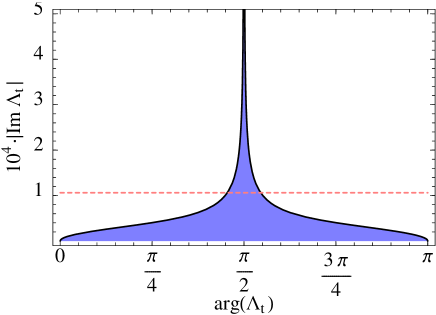
Figure 3: Limit on $|\mathop{\mbox{Im}}\Lambda_{t}|$ imposed by $\Delta m_{K}$ and $\varepsilon_{K}$, through RGE evolution, as a function of $\arg\Lambda_{t}$. The dashed line shows the SM contribution to $\mathop{\mbox{Im}}Z_{ds}$ for $\mathop{\mbox{Im}}\lambda_{t}=1.33\cdot 10^{-4}$.

As we shall discuss in the next section, this particular case can be tested experimentally in a clear way by studying rare $K$ decays: if for example BR$(K_{L}\to\pi^{0}\nu\bar{\nu})$ will be found to agree with the SM expectations, then the possibility of a large $\mathop{\mbox{Im}}\Lambda_{t}$ will be ruled out.

The constraints we considered on the relevant mass insertions can be evaded in corners of parameter space, but this holds only if an unlikely fine-tuning is allowed. For example the limits from $\Delta m_{K}$ and $\varepsilon_{K}$ can be evaded if there is a cancellation among the different supersymmetric contributions to them, or the limit from RGE can be evaded if there is a cancellation between the initial value of the insertion and the RGE contribution.

Since the insertions are pushed up to their experimental limits the results plotted should not of course be considered as predictions but just as maximal possible effects. Our framework is in fact general enough to include any supersymmetric extensions of the SM with minimal field content. This on one hand insures that we are not missing potentially large effects. On the other hand, one might ask whether values of $|\mathop{\mbox{Im}}\Lambda_{t}|$ as large as those ones in the shaded region of Fig. 3 naturally arise in supersymmetric models. Unfortunately, within the most common models this is not the case, as we will now briefly show.

Explicit models account for the strong constraints on soft supersymmetry breaking terms in different ways. In some cases the mechanism communicating the supersymmetry breaking guarantees that FCNC and CP-violating processes are under control. This is the case e.g. of gauge mediated supersymmetry breaking and of minimal supergravity (SUGRA). In other cases, further ingredients are necessary.

In the minimal situations, a quick estimate yields

$$\Lambda_{t} \sim 0.3\cdot 10^{-2}\lambda_{t}\frac{H_{0}(x_{q\chi})}{H_{0}(1)}\left(\frac{300\,{\rm GeV}}{m^{\prime}_{S}}\right)^{2}$$ (65)

$$\Lambda^{\pm}_{g} \sim 0.3\cdot 10^{-4}\lambda_{t}\frac{G_{0}(x_{gq})}{G_{0}(1)}\left(\frac{300\,{\rm GeV}}{m^{\prime\prime}_{S}}\right),$$ (66)

where $M_{X}\sim 10^{16}$ has been used to estimate $\Lambda_{g}^{\pm}$ and $m^{\prime}_{S}$, $m^{\prime\prime}_{S}$ are dimensionful combinations of diagonal soft parameters. Eqs. (65) and (66) show that $\Lambda_{t}$ and $\Lambda_{g}^{\pm}$ give rise to negligible effects compared to the SM ones.

On the other hand the universality hypothesis used in minimal SUGRA has not a compelling justification. In this and other cases in which the mechanism generating the soft terms does not guarantee that FCNC are under control, the potential FCNC problem must be solved by further symmetries. From this point of view the issue of why the scalar mass eigenstates are so degenerate or so aligned with the corresponding fermion eigenstates is the supersymmetric version of the issue of explaining the structure of fermion masses and mixings. If the latter is accounted for by flavour symmetries acting on the fermion generation indices, in a supersymmetric theory the same symmetry acts on the corresponding scalar indices. As a consequence, whatever is the symmetry, since the Yukawa and the corresponding soft trilinear interactions have the same quantum numbers, the structure of their coupling matrices is the same. Within this class of models it is therefore possible to show that the LR mass insertions involving the third generation, and in turn the double insertion, are similar to those obtained in the minimal models. This is not what happens for $(\delta^{D}_{LR})_{12}$, that can be shown to be of the right order of magnitude to generate the experimental value of $\varepsilon^{\prime}/\varepsilon$ [11]. Therefore the most likely situation, as far as the most common SUSY models are concerned, is somewhere between the case of $\Lambda_{t}\simeq 0$ and $\Lambda_{g}\neq 0$ and the case of $\Lambda_{t}=\Lambda_{g}=0$. We stress, however, that the flavor structure of the supersymmetry breaking is far from having been established. It is then worthwhile to investigate also more exotic possibilities, like the one of a large $\mathop{\mbox{Im}}\Lambda_{t}$, as far as these are not ruled out by phenomenological constraints.

6 Numerical Analysis

6.1 Strategy

We are now ready to discuss magnitude and relations among possible supersymmetric contributions to $\varepsilon^{\prime}/\varepsilon$ and rare decays. To this purpose it is useful to distinguish between three basic scenarios:

Scenario A: $[\mathop{\mbox{Im}}\Lambda_{t}=0,\ \mathop{\mbox{Im}}\Lambda_{g}^{\pm}\not=0]$.
This scenario is close to what happens in most SUSY models since, as we have seen in the previous section, the $\bar{s}dZ$ vertex can receive sizable corrections only in a specific region of the parameter space. In this case $\varepsilon^{\prime}/\varepsilon$ can be affected only by the chromomagnetic operator and, as shown in Section 4.3, among the rare modes only $K_{L}\to\pi^{0}e^{+}e^{-}$ is sensitive to this SUSY contribution. On the other hand if $\mathop{\mbox{Re}}\Lambda_{t}$ is substantially different from zero also $K^{+}\to\pi^{+}\nu\bar{\nu}$ can be significantly affected.

Scenario B: $[\mathop{\mbox{Im}}\Lambda_{t}\not=0,\ \mathop{\mbox{Im}}\Lambda_{g}^{\pm}=0]$.
In this scenario the possibility of large corrections to $\varepsilon^{\prime}/\varepsilon$ is not favoured from the point of view of the parameter space, but is an interesting possibility to be investigated in a model-independent approach. If this is the case, sizable effects are then expected both in $K_{L}\to\pi^{0}\nu\bar{\nu}$ and $K_{L}\to\pi^{0}e^{+}e^{-}$.

Scenario C: $[\mathop{\mbox{Im}}\Lambda_{t}\not=0,\ \mathop{\mbox{Im}}\Lambda_{g}^{\pm}\not=0]$.
This represents the most general case. Note, however, that the requirement of having sizable cancellations in $\varepsilon^{\prime}/\varepsilon$, between supersymmetric contributions generated by the chromomagnetic operator and the $\bar{s}dZ$ vertex, implies an additional fine-tuning with respect to scenarios A and B.

We will also follow [15] and consider three scenarios for $\lambda_{t}$, which enter Standard Model contributions and its interference with supersymmetric contributions to rare decays and $\varepsilon^{\prime}/\varepsilon$. Indeed there is the possibility that the value of $\lambda_{t}$ is modified by new contributions to $\varepsilon$ and $B_{d,s}^{0}-\bar{B}_{d,s}^{0}$ mixings. We consider therefore three scenarios:

• Scenario I: $\lambda_{t}$ is taken from the standard analysis of the unitarity triangle and varied in the ranges:

  $$1.05\cdot 10^{-4}\leq\mathop{\mbox{Im}}\lambda_{t}\leq 1.61\cdot 10^{-4}$$ (67)

  $$2.3\cdot 10^{-4}\leq-\mathop{\mbox{Re}}\lambda_{t}\leq 3.8\cdot 10^{-4}$$ (68)

• Scenario II: $\mathop{\mbox{Im}}\lambda_{t}=0$ and $\mathop{\mbox{Re}}\lambda_{t}$ is varied in the full range consistent with the unitarity of the CKM matrix:

  $$1.61\cdot 10^{-4}\leq-\mathop{\mbox{Re}}\lambda_{t}\leq 5.6\cdot 10^{-4}$$ (69)

  In this scenario CP violation comes entirely from new physics contributions.

• Scenario III: $\lambda_{t}$ is varied in the full range consistent with the unitarity of the CKM matrix:

  $$-1.73\cdot 10^{-4}\leq\mathop{\mbox{Im}}\lambda_{t}\leq 1.73\cdot 10^{-4}$$ (70)

  This means in particular that $\mathop{\mbox{Im}}\lambda_{t}$ can be negative.

We would like to emphasize that the scenarios II and in particular III are very unlikely and are presented here only for completeness. We stress that if one uses the Standard Model expressions for $B^{0}-\bar{B}^{0}$ mixings, $\varepsilon_{K}$ and $\sin 2\beta$ one gets results for the CKM matrix which are compatible with the $|V_{ub}/V_{cb}|$ constraint, which is insensitive to new physics. In view of the coherence of the Standard Model picture, corrections to the processes in question so large as to make $\mathop{\mbox{Im}}\lambda_{t}$ negative, or $\mathop{\mbox{Re}}\lambda_{t}$ way outside the range in Eq. (68) look rather improbable. We believe that if the new physics has an impact on the usual determination of $\lambda_{t}$, the most likely situation is between scenarios I and II.

6.2 $\varepsilon^{\prime}/\varepsilon$

We shall now proceed extracting ranges for the effective SUSY couplings from the experimental data on $\varepsilon^{\prime}/\varepsilon$ in the basic scenarios A-C defined above. These will then be used to estimate the branching ratios of the rare decay modes.

Assuming that the SM contribution to $\mathop{\mbox{Re}}(\varepsilon^{\prime}/\varepsilon)$ is around its central value, as given in [5], and therefore much smaller than the experimental result, there is a lot of room for SUSY to contribute to this quantity. Detailed bounds on $\mathop{\mbox{Re}}(\varepsilon^{\prime}/\varepsilon)^{{}^{\rm SUSY}}$ depend on the various parameters entering $\mathop{\mbox{Re}}(\varepsilon^{\prime}/\varepsilon)^{{}^{\rm SM}}$, as well as on the experimental result in (2), however, as a simplified starting point for our discussion, we assume at first

$$\mathop{\mbox{Re}}\left(\frac{\varepsilon^{\prime}}{\varepsilon}\right)^{\mbox{\tiny SUSY}}=2\cdot 10^{-3}~{}.$$ (71)

This value has to be taken only as a reference figure: it could be interpreted either as the difference between the experimental result and the SM contribution or as the true value of $\mathop{\mbox{Re}}(\varepsilon^{\prime}/\varepsilon)$ in the limit of a real CKM matrix.

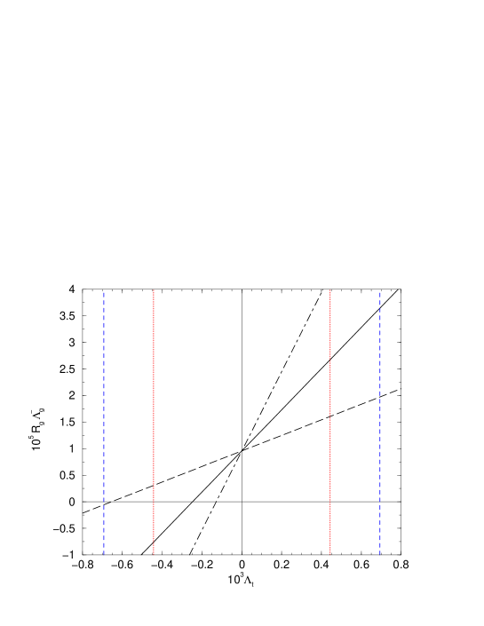
Figure 4: Linear relation between $\Lambda_{g}^{-}$ and $\Lambda_{t}$ for $\mathop{\mbox{Re}}(\varepsilon^{\prime}/\varepsilon)^{{}^{\rm SUSY}}=2\cdot~{}10^{-3}$. The solid line is for $\{B_{8}^{(3/2)},R_{s},r_{Z}^{(8)}\}=\{0.8,1.5,7.8\}$, the dot-dashed for $\{B_{8}^{(3/2)},R_{s},r_{Z}^{(8)}\}=\{1.0,2.0,8.4\}$ and the dashed for $\{B_{8}^{(3/2)},R_{s},r_{Z}^{(8)}\}=\{0.6,1.0,7.1\}$. The vertical lines show the RGE bound (64) for $m_{\tilde{q}}=300$ GeV and $\{x_{q\chi},x_{gq}\}=\{3,1\}$ (dotted) or $\{x_{q\chi},x_{gq}\}=\{9,1.3\}$ (dashed).

Since our formula for the SUSY contribution Eq. (33) contains only two free parameters, $\mathop{\mbox{Im}}\Lambda_{t}$ and $\mathop{\mbox{Im}}\Lambda^{-}_{g}$, Eq. (71) defines a straight line in the $(\mathop{\mbox{Im}}\Lambda_{t},\mathop{\mbox{Im}}\Lambda^{-}_{g})$ plane, which represents the general solution within scenario C. This is shown in Fig. 4 for three different sets of $\{B_{8}^{(3/2)},R_{s},r_{Z}^{(8)}\}$. Decreasing the reference value in (71) corresponds to a translation of the straight lines toward the origin; the intercepts of the lines with vertical and horizontal axes define the solutions within scenarios A and B, respectively.

As it can be noticed, if $\Lambda^{-}_{g}=0$, then $\mathop{\mbox{Im}}\Lambda_{t}$ must be negative, i.e. the SUSY contribution to the $\bar{s}dZ$ vertex must be opposite to the SM one in order to produce a positive contribution to $\varepsilon^{\prime}/\varepsilon$. The minimum value of $|\mathop{\mbox{Im}}\Lambda_{t}|$ with $\Lambda^{-}_{g}=0$ is found for the maximum values of $B_{8}^{(3/2)}$, $R_{s}$ and $r_{Z}^{(8)}$. In this case SUSY and SM contributions to the $\bar{s}dZ$ vertex cancel almost completely and the experimental value for $\varepsilon^{\prime}/\varepsilon$ is roughly reproduced by QCD penguin contributions. On the other hand, the maximum allowed value of $|\mathop{\mbox{Im}}\Lambda_{t}|$ with $\Lambda^{-}_{g}=0$ is found for the minimum set of $\{B_{8}^{(3/2)},R_{s},r_{Z}^{(8)}\}$. In this case the $\bar{s}dZ$ vertex has an opposite sign with respect to the SM case and is largely dominated by SUSY contributions ($|Z_{ds}/Z^{\rm SM}_{ds}|\stackrel{{\scriptstyle>}}{{{}_{\sim}}}6)$. This solution is still allowed by the RGE constraint (64), provided the sparticle masses are not too high. The situation of course changes if one allows also $\mathop{\mbox{Im}}\Lambda^{-}_{g}$ to be different from zero. In particular, for large ($\stackrel{{\scriptstyle>}}{{{}_{\sim}}}10^{-5}$) and positive values of $R_{g}\mathop{\mbox{Im}}\Lambda^{-}_{g}$ a positive $\mathop{\mbox{Im}}\Lambda_{t}$ is needed in order to avoid too large effects in $\varepsilon^{\prime}/\varepsilon$.

In the limit where the standard determination of the CKM matrix is valid, a quantitative estimate of the ranges for $\mathop{\mbox{Im}}\Lambda^{-}_{g}$ and $\mathop{\mbox{Im}}\Lambda_{t}$, within scenarios A and B, can be obtained by subtracting the SM contribution from the experimental value in (2). Following [15], we parametrize the SM result for $\varepsilon^{\prime}/\varepsilon$ using the approximate formula

$$\mathop{\mbox{Re}}\left(\frac{\varepsilon^{\prime}}{\varepsilon}\right)^{\mbox{\tiny SM}}=\mathop{\mbox{Im}}\lambda_{t}\biggl{[}-1.4+R_{s}\Bigl{[}1.1|r_{Z}^{(8)}|B_{6}^{(1/2)}+(1.0-0.67|r_{Z}^{(8)}|)B_{8}^{(3/2)}\Bigr{]}\biggr{]}\,$$ (72)

with [5]

$$\mathop{\mbox{Im}}\lambda_{t}=(1.33\pm 0.14)\cdot 10^{-4}~{}.$$ (73)

Varying $\mathop{\mbox{Im}}\lambda_{t}$ and the experimental value (2) within $2\sigma$ intervals, choosing $B_{8}^{(3/2)}$, $R_{s}$ and $r_{Z}^{(8)}$ as discussed in Section 4.2 and, finally, assuming $0.7\leq B^{(1/2)}_{6}\leq 1.3$, we find:

$$-15.5\cdot 10^{-4}\leq \mathop{\mbox{Re}}\left(\frac{\varepsilon^{\prime}}{\varepsilon}\right)^{\mbox{\tiny SUSY}} \leq 30.1\cdot 10^{-4}\;,$$ (74)

$$-9.3\cdot 10^{-4}\leq \mathop{\mbox{Im}}\Lambda_{t} \leq 1.7\cdot 10^{-4}\qquad(\mathop{\mbox{Im}}\Lambda_{g}^{-}=0)\;,$$ (75)

$$-0.7\cdot 10^{-5}\leq R_{g}\mathop{\mbox{Im}}\Lambda_{g}^{-} \leq 1.4\cdot 10^{-5}\qquad(\mathop{\mbox{Im}}\Lambda_{t}=0)\;.$$ (76)

It is interesting to note that the range of $\mathop{\mbox{Im}}\Lambda_{g}^{-}$ is well within the bound (52), therefore $\varepsilon^{\prime}/\varepsilon$ provides the most stringent bound on $|\mathop{\mbox{Im}}\Lambda_{g}^{-}|$ within scenario A. Similarly, $\varepsilon^{\prime}/\varepsilon$ provides the most stringent model-independent upper bound on $\mathop{\mbox{Im}}\Lambda_{t}$ within scenario B. On the other hand, the lower bound on $\mathop{\mbox{Im}}\Lambda_{t}$ imposed by $\varepsilon^{\prime}/\varepsilon$ is weaker than the bound (64) for $m_{\tilde{q}}\stackrel{{\scriptstyle>}}{{{}_{\sim}}}200$  GeV and $x_{gq}<1.3$.

To show the possible improvement due to more precise measurement of $\varepsilon^{\prime}/\varepsilon$ we show how (74)–(76) are modified if we fix $\mathop{\mbox{Re}}(\varepsilon^{\prime}/\varepsilon)_{\rm exp}=20\cdot 10^{-4}$. We find

$$-7.5\cdot 10^{-4}\leq \mathop{\mbox{Re}}\left(\frac{\varepsilon^{\prime}}{\varepsilon}\right)^{\mbox{\tiny SUSY}} \leq 19.7\cdot 10^{-4}\;,$$ (77)

$$-5.9\cdot 10^{-4}\leq \mathop{\mbox{Im}}\Lambda_{t} \leq 0.8\cdot 10^{-4}\qquad(\mathop{\mbox{Im}}\Lambda_{g}^{-}=0)\;,$$ (78)

$$-0.4\cdot 10^{-5}\leq R_{g}\mathop{\mbox{Im}}\Lambda_{g}^{-} \leq 0.9\cdot 10^{-5}\qquad(\mathop{\mbox{Im}}\Lambda_{t}=0)\;.$$ (79)

6.3 Rare Decays

The rare decays $K_{L}\to\pi^{0}\nu\bar{\nu}$ and $K_{L}\to\pi^{0}e^{+}e^{-}$ provide in principle a powerful tool to clearly establish possible SUSY contributions in $CP$-violating $|\Delta S|=1$ amplitudes, and also to distinguish among the three scenarios introduced in Section 6.1.

6.3.1 Scenario A

Within scenario A only $K_{L}\to\pi^{0}e^{+}e^{-}$ among these two modes is affected by SUSY corrections. Setting $R_{\alpha_{s}}=1$ in (32) we can write

$$\mathop{\mbox{Im}}\Lambda_{g}^{+}{\tilde{y}_{\gamma}}=35.5~{}R_{g}\mathop{\mbox{Im}}\Lambda_{g}^{-}~{}\left[\frac{\mathop{\mbox{Im}}\Lambda_{g}^{+}}{\mathop{\mbox{Im}}\Lambda_{g}^{-}}\right]~{}\left[\frac{B_{T}}{B_{G}\sqrt{R_{S}}}\right]~{},$$ (80)

where the numerical coefficient has been obtained for $x_{gq}=1$ and can increase at most to 37.0 if we impose $x_{gq}<1.3$. Assuming $R_{g}\mathop{\mbox{Im}}\Lambda_{g}^{-}=10^{-5}$, as obtained from Fig. 4, and fixing to unit the two ratios among square brackets in (80), we obtain $\mathop{\mbox{Im}}\Lambda_{g}^{+}{\tilde{y}_{\gamma}}=3.5\cdot 10^{-4}$. Using this figure in (43) we find that the additional contribution to ${\rm BR}(K_{L}\to\pi^{0}e^{+}e^{-})_{\rm dir}$ is positive and ranges between 3 and 4 in units of $10^{-12}$, depending on the value of $\mathop{\mbox{Im}}\lambda_{t}$. This effect, which represents the typical size of the SUSY contribution to $K_{L}\to\pi^{0}e^{+}e^{-}$ expected within scenario A, is certainly difficult to be observed. However, we stress that this conclusion depends strongly on the assumptions made for $\mathop{\mbox{Im}}\Lambda_{g}^{+}/\mathop{\mbox{Im}}\Lambda_{g}^{-}$ and $B_{T}/(B_{G}\sqrt{R_{S}})$.

According to the ranges of $B_{T}$, $B_{G}$ and $R_{s}$ discussed in Section 4, we expect

$$0.09\leq\frac{B_{T}}{B_{G}\sqrt{R_{S}}}\leq 2\;.$$ (81)

On the other hand, it is more difficult to estimate $\mathop{\mbox{Im}}\Lambda_{g}^{+}/\mathop{\mbox{Im}}\Lambda_{g}^{-}$ without specific assumptions on the SUSY soft-breaking terms. In minimal models it is natural to assume $(\delta^{D}_{LR})_{12}\gg(\delta^{D}_{LR})_{21}$, that implies

$$\frac{\mathop{\mbox{Im}}\Lambda_{g}^{+}}{\mathop{\mbox{Im}}\Lambda_{g}^{-}}\simeq-1\;,$$ (82)

but we cannot exclude sizable deviations from this figure in generic scenarios.

In Table 1 we report the upper bounds on ${\rm BR}(K_{L}\to\pi^{0}e^{+}e^{-})_{\rm dir}$, for different values of the two ratios. To this end we have used the expressions for $\varepsilon^{\prime}/\varepsilon$ and ${\rm BR}(K_{L}\to\pi^{0}e^{+}e^{-})_{\rm dir}$ given in Section 4 with the Standard Model contribution for $\varepsilon^{\prime}/\varepsilon$ given in (72). Scanning the parameters $B_{8}^{(3/2)}$, $B^{(1/2)}_{6}$, $R_{s}$ and $r_{Z}^{(8)}$ as discussed in Section 4.2 and 6.2, varying $\mathop{\mbox{Im}}\lambda_{t}$ according to (67) (scenario I), we find the results in the third and fourth column which correspond to two choices of $\varepsilon^{\prime}/\varepsilon$. As it can be noticed, results in the ball park of $10^{-11}$ cannot be excluded even under the assumption (82).

$\mathop{\mbox{Im}}\Lambda_{g}^{+}/\mathop{\mbox{Im}}\Lambda_{g}^{-}$	$B_{T}/(B_{G}\sqrt{R_{S}})$	${\rm BR}(K_{L}\to\pi^{0}e^{+}e^{-})_{\rm dir}$	${\rm BR}(K_{L}\to\pi^{0}e^{+}e^{-})_{\rm dir}$
-1	1.0	$9.4\cdot 10^{-12}$	$7.8\cdot 10^{-12}$
-1	0.5	$7.8\cdot 10^{-12}$	$7.0\cdot 10^{-12}$
-1	1.5	$1.1\cdot 10^{-11}$	$8.5\cdot 10^{-12}$
-2	1.5	$1.8\cdot 10^{-11}$	$1.1\cdot 10^{-11}$
1	1.0	$1.3\cdot 10^{-11}$	$1.0\cdot 10^{-11}$
1	0.5	$9.3\cdot 10^{-12}$	$8.2\cdot 10^{-12}$
1	1.5	$1.8\cdot 10^{-11}$	$1.3\cdot 10^{-11}$
2	1.5	$3.7\cdot 10^{-11}$	$2.3\cdot 10^{-11}$

Table 1: Upper bounds on ${\rm BR}(K_{L}\to\pi^{0}e^{+}e^{-})_{\rm dir}$ within scenario A, for different values of $\mathop{\mbox{Im}}\Lambda_{g}^{+}/\mathop{\mbox{Im}}\Lambda_{g}^{-}$ and $B_{T}/(B_{G}\sqrt{R_{S}})$ consistent with $12\leq 10^{4}\mathop{\mbox{Re}}(\varepsilon^{\prime}/\varepsilon)\leq 30.4$ (third column) and $\mathop{\mbox{Re}}(\varepsilon^{\prime}/\varepsilon)=20.0\cdot 10^{-4}$ (fourth column). The bounds are obtained setting $x_{gq}=1.3$ in order to maximize the numerical coefficient in (80). To maximize the interference of SM and SUSY amplitudes, $R_{g}\mathop{\mbox{Im}}\Lambda_{g}^{-}$ is chosen as the maximum (minimum) value allowed by $\varepsilon^{\prime}/\varepsilon$ for positive (negative) $\mathop{\mbox{Im}}\Lambda_{g}^{+}/\mathop{\mbox{Im}}\Lambda_{g}^{-}$.

$\mathop{\mbox{Im}}\Lambda_{g}^{+}/\mathop{\mbox{Im}}\Lambda_{g}^{-}$	${\rm BR}(K_{L}\to\pi^{0}e^{+}e^{-})_{\rm dir}$ (II)	${\rm BR}(K_{L}\to\pi^{0}e^{+}e^{-})_{\rm dir}$ (III)
-1	1.8 (0.8) $\cdot 10^{-12}$	2.5 (2.1) $\cdot 10^{-11}$
-2	7.3 (3.2) $\cdot 10^{-12}$	5.7 (4.5) $\cdot 10^{-11}$
1	1.8 (0.8) $\cdot 10^{-12}$	1.5 (1.2) $\cdot 10^{-11}$
2	7.3 (3.2) $\cdot 10^{-12}$	2.5 (1.7) $\cdot 10^{-11}$

Table 2: Upper bounds on ${\rm BR}(K_{L}\to\pi^{0}e^{+}e^{-})_{\rm dir}$ within scenario A for $\mathop{\mbox{Im}}\lambda_{t}=0$ (II) and $|\mathop{\mbox{Im}}\lambda_{t}|<1.73\cdot 10^{-4}$ (III). The bounds are obtained setting $B_{T}/(B_{G}\sqrt{R_{S}})=1$ and imposing $\mathop{\mbox{Re}}(\varepsilon^{\prime}/\varepsilon)\leq 30.4(20.0)\cdot 10^{-4}$.

The dependence of ${\rm BR}(K_{L}\to\pi^{0}e^{+}e^{-})_{\rm dir}$ on the value of $\mathop{\mbox{Im}}\lambda_{t}$ is shown in Table 2. If the CKM matrix is real and $|(\mathop{\mbox{Im}}\Lambda_{g}^{+}/\mathop{\mbox{Im}}\Lambda_{g}^{-})B_{T}/(B_{G}\sqrt{R_{S}})|\stackrel{{\scriptstyle>}}{{{}_{\sim}}}1$, we find ${\rm BR}(K_{L}\to\pi^{0}e^{+}e^{-})_{\rm dir}\sim{\rm few}\times 10^{-12}$, similarly to the SM case. On the other hand values substantially larger than $10^{-11}$ are obtained within scenario III. Note, however, that the large results quoted for $\mathop{\mbox{Im}}\Lambda_{g}^{+}/\mathop{\mbox{Im}}\Lambda_{g}^{-}<0$ are very unlikely, since are obtained for the maximum negative value of $\mathop{\mbox{Im}}\lambda_{t}$.

Concerning $K_{L}\to\pi^{0}\nu\bar{\nu}$, its branching ratio in scenario A stays close to the Standard Model value provided the usual determination of $\mathop{\mbox{Im}}\lambda_{t}$ is not substantially decreased through supersymmetric contributions to $\varepsilon_{K}$. Because of the unitarity of the CKM matrix $\mathop{\mbox{Im}}\lambda_{t}$ can only be marginally increased over its SM value. On the other hand if $\mathop{\mbox{Im}}\lambda_{t}=0$ a clear signature for scenario A would be a vanishingly small ${\rm BR}(K_{L}\to\pi^{0}\nu\bar{\nu})$ ($\stackrel{{\scriptstyle<}}{{{}_{\sim}}}10^{-14}$ [30]).

The case of $K^{+}\to\pi^{+}\nu\bar{\nu}$ is different as it is dominantly governed by $\mathop{\mbox{Re}}\lambda_{t}$ and $\mathop{\mbox{Re}}\Lambda_{t}$. The upper bound on ${\rm BR}(K^{+}\to\pi^{+}\nu\bar{\nu})$ can be obtained by using equation (49) together with the bound [16, 31, 32, 15]

$${\rm BR}(K_{L}\to\mu^{+}\mu^{-})_{\rm SD}\leq 2.8\cdot 10^{-9}$$ (83)

i.e. $\kappa=2.8$. Choosing then $(-\mathop{\mbox{Re}}\lambda_{t})_{\rm max}=3.8\cdot 10^{-4}$ (scenario I for $\lambda_{t})$, as obtained in the Standard Model, or $(-\mathop{\mbox{Re}}\lambda_{t})_{\rm max}=5.6\cdot 10^{-4}$ (scenarios II and III), we find respectively

$${\rm BR}(K^{+}\to\pi^{+}\nu\bar{\nu})\leq 1.70\cdot 10^{-10}+0.229{\rm BR}(K_{L}\to\pi^{0}\nu\bar{\nu})~{},$$ (84)

$${\rm BR}(K^{+}\to\pi^{+}\nu\bar{\nu})\leq 2.03\cdot 10^{-10}+0.229{\rm BR}(K_{L}\to\pi^{0}\nu\bar{\nu})$$ (85)

As the second terms on the r.h.s of these bounds are very small in this scenario we find ${\rm BR}(K^{+}\to\pi^{+}\nu\bar{\nu})\leq 1.7\cdot 10^{-10}$ and ${\rm BR}(K^{+}\to\pi^{+}\nu\bar{\nu})\leq 2.1\cdot 10^{-10}$. These results are also obtained if $\mathop{\mbox{Re}}\Lambda_{t}$ is varied in the full range consistent with the bound (83) and with the RGE constraint (88) with $\mathop{\mbox{Im}}\Lambda_{t}=0$. Evidently as (84) and (85) have been obtained without the constraint (88), what matters in this scenario is (83).

6.3.2 Scenario B

Being strongly sensitive to $\mathop{\mbox{Im}}\Lambda_{t}$ and insensitive to $\mathop{\mbox{Im}}\Lambda_{g}^{\pm}$, $K_{L}\to\pi^{0}\nu\bar{\nu}$ represents the golden mode to identify scenarios B and C. We first discuss scenario B which corresponds to the case analyzed in [15]. This time, however, the effective $\bar{s}dZ$ vertex is additionally constrained by the renormalization group analysis of Section 5.

The dependence of ${\rm BR}(K_{L}\to\pi^{0}\nu\bar{\nu})$ on $\mathop{\mbox{Im}}\Lambda_{t}$ is shown in the left plot of Fig. 5. As can be noticed, large enhancements with respect to the SM case are possible, but on the other hand we cannot exclude a destructive interference among SUSY and SM contributions leading to strong suppression of ${\rm BR}(K_{L}\to\pi^{0}\nu\bar{\nu})$.

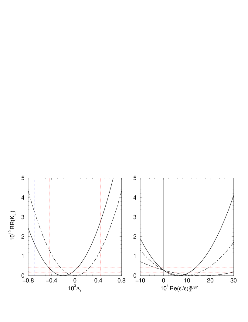
Figure 5: ${\rm BR}(K_{L}\rightarrow\pi^{0}\nu\bar{\nu}$) as a function of $\mathop{\mbox{Im}}\Lambda_{t}$ (left) or as a function of $(\varepsilon^{\prime}/\varepsilon)_{Z}^{{}^{\rm SUSY}}$ (right). In the left plot the solid (dot-dashed) parabola is for $\mathop{\mbox{Im}}\lambda_{t}=1.33\cdot 10^{-4}$ (0) and the vertical lines show the RGE bounds as in Fig. 4. In the right plot the three parabola are for $\mathop{\mbox{Im}}\lambda_{t}=1.33\cdot 10^{-4}$ and $\{B_{8}^{(3/2)},R_{s},r_{Z}^{(8)}\}=\{0.6,1.0,7.1\}$ (solid), $\{B_{8}^{(3/2)},R_{s},r_{Z}^{(8)}\}=\{0.7,1.0,7.8\}$ (dot-dashed) or $\{B_{8}^{(3/2)},R_{s},r_{Z}^{(8)}\}=\{0.8,1.5,7.8\}$ (dashed). In both cases the horizontal lines denote the SM range of ${\rm BR}(K_{L}\rightarrow\pi^{0}\nu\bar{\nu}$) for $1.05<10^{4}\mathop{\mbox{Im}}\lambda_{t}<1.61$.

If the standard determination of $\mathop{\mbox{Im}}\lambda_{t}$ is valid, Eq. (42) implies that ${\rm BR}(K_{L}\rightarrow\pi^{0}\nu\bar{\nu})$ can be enhanced with respect to the SM case only if

$$\mathop{\mbox{Im}}\Lambda_{t}<-2X_{0}\mathop{\mbox{Im}}\lambda_{t}\qquad{\rm or}\qquad\mathop{\mbox{Im}}\Lambda_{t}>0~{}.$$ (86)

The second possibility is excluded within scenario B if we require a positive SUSY contribution to $\varepsilon^{\prime}/\varepsilon$. This is clearly shown by the second plot in Fig. 5, which illustrates the relation between ${\rm BR}(K_{L}\rightarrow\pi^{0}\nu\bar{\nu})$ and the SUSY contribution to $\varepsilon^{\prime}/\varepsilon$ within scenario B, assuming the standard determination of $\mathop{\mbox{Im}}\lambda_{t}$. In this case large enhancements of ${\rm BR}(K_{L}\rightarrow\pi^{0}\nu\bar{\nu})$ are possible, but only if $R_{s}$ and $B_{8}$ are close to their minimum values. On the other hand, if $R_{s}$ and/or $B_{8}$ are large, then ${\rm BR}(K_{L}\rightarrow\pi^{0}\nu\bar{\nu})$ is more likely to be suppressed rather than enhanced with respect to the SM case.

In order to be more quantitative we consider the three scenarios for $\lambda_{t}$ defined at the beginning of this section. Next, as discussed in Section 6.2, $\mathop{\mbox{Im}}\Lambda_{t}$ can be best bounded by $\varepsilon^{\prime}/\varepsilon$ and the renormalization group analysis of Section 5. $\mathop{\mbox{Re}}\Lambda_{t}$ can be bounded by the present information on the short distance contribution to $K_{L}\to\mu^{+}\mu^{-}$ and also by the RG analysis of Section 5, as we will state more explicitly below. These bounds imply a bound on ${\rm BR}(K^{+}\to\pi^{+}\nu\bar{\nu})$. Since ${\rm BR}(K^{+}\to\pi^{+}\nu\bar{\nu})$ depends on both $\mathop{\mbox{Re}}\Lambda_{t}$ and $\mathop{\mbox{Im}}\Lambda_{t}$ also the bound on $\mathop{\mbox{Im}}\Lambda_{t}$ matters in cases where it is substantially larger than the Standard Model contribution to $\mathop{\mbox{Im}}Z_{ds}$.

The branching ratios ${\rm BR}(K_{L}\to\pi^{0}\nu\bar{\nu})$ and ${\rm BR}(K_{L}\to\pi^{0}e^{+}e^{-})_{\rm dir}$ are dominated by $(\mathop{\mbox{Im}}Z_{sd})^{2}$. Yet, the outcome of this analysis depends sensitively on the sign of $\mathop{\mbox{Im}}Z_{sd}$. Indeed, $\mathop{\mbox{Im}}Z_{sd}>0$ results in the suppression of $\varepsilon^{\prime}/\varepsilon$ and since in the Standard Model the value for $\varepsilon^{\prime}/\varepsilon$ is generally below the data, substantial enhancements of $\mathop{\mbox{Im}}Z_{sd}$ with $\mathop{\mbox{Im}}Z_{sd}>0$ are not possible. The situation changes if new physics reverses the sign of $\mathop{\mbox{Im}}Z_{sd}$ so that it becomes negative. Then the upper bound on $-\mathop{\mbox{Im}}Z_{sd}$ is governed by the upper bound on $\varepsilon^{\prime}/\varepsilon$ and with suitable choice of hadronic parameters and $\mathop{\mbox{Im}}\lambda_{t}$ (in particular in scenario III) large enhancements of $-\mathop{\mbox{Im}}Z_{sd}$ and of rare decay branching ratios are in principle possible. The largest branching ratios are found when the neutral meson mixing is dominated by new physics contributions which force $\mathop{\mbox{Im}}\lambda_{t}$ to be as negative as possible within the unitarity of the CKM matrix. As we argued above, this possibility is quite remote. However, if this situation could be realized in some exotic model, then the branching ratios in question could be very high as demonstrated in [15].

In this context it is interesting to observe that in the case of supersymmetry such large enhancements of $-\mathop{\mbox{Im}}Z_{sd}$ while allowed by $\varepsilon^{\prime}/\varepsilon$ are ruled out by the renormalization group bound on $\mathop{\mbox{Im}}\Lambda_{t}$ considered in Section 5. As we will see in a moment the imposition of the bound (see Fig. 3)

$$|\mathop{\mbox{Im}}\Lambda_{t}|\leq 5.0\cdot 10^{-4}$$ (87)

has in the case of a negative $\mathop{\mbox{Im}}\Lambda_{t}$ a very large impact on the analysis in [15] suppressing considerably the upper bounds on rare decays obtained there.

$10^{4}\mathop{\mbox{Re}}(\varepsilon^{\prime}/\varepsilon)_{\rm min}$	Scenario for $\lambda_{t}$:	I	II	III	SM
	$10^{10}~{}{\rm BR}(K_{L}\to\pi^{0}\nu\bar{\nu})$	$1.2~{}(0.6)$	$-$	$1.4~{}(0.8)$	0.4
12.0	$10^{11}~{}{\rm BR}(K_{L}\to\pi^{0}e^{+}e^{-})_{\rm dir}$	$1.7~{}(0.9)$	$-$	$2.1~{}(1.1)$	0.7
	$10^{10}~{}{\rm BR}(K^{+}\to\pi^{+}\nu\bar{\nu})^{*}$	$2.0~{}(1.8)$	$-$	$2.4~{}(2.2)$	1.1
	$10^{10}~{}{\rm BR}(K^{+}\to\pi^{+}\nu\bar{\nu})$	$1.7~{}(1.7)$	$-$	$2.1~{}(1.9)$	1.1
	$10^{10}~{}{\rm BR}(K_{L}\to\pi^{0}\nu\bar{\nu})$	$0.7~{}(0.4)$	$-$	$0.9~{}(0.5)$	0.4
20.0	$10^{11}~{}{\rm BR}(K_{L}\to\pi^{0}e^{+}e^{-})_{\rm dir}$	$1.1~{}(0.7)$	$-$	$1.3~{}(0.8)$	0.7
	$10^{10}~{}{\rm BR}(K^{+}\to\pi^{+}\nu\bar{\nu})^{*}$	$1.9~{}(1.8)$	$-$	$2.2~{}(2.2)$	1.1
	$10^{10}~{}{\rm BR}(K^{+}\to\pi^{+}\nu\bar{\nu})$	$1.7~{}(1.7)$	$-$	$2.0~{}(1.9)$	1.1

Table 3: Upper bounds for the branching ratios of the rare decays $K_{L}\to\pi^{0}\nu\bar{\nu}$, $K_{L}\to\pi^{0}e^{+}e^{-}$ and $K^{+}\to\pi^{+}\nu\bar{\nu}$ in the case $\mathop{\mbox{Im}}\Lambda_{t}>0$, $\mathop{\mbox{Im}}\Lambda^{\pm}_{g}=0$. The results have been obtained in various scenarios for $\lambda_{t}$ by imposing $\mathop{\mbox{Re}}(\varepsilon^{\prime}/\varepsilon)\geq 12.0\cdot 10^{-4}$ or $\mathop{\mbox{Re}}(\varepsilon^{\prime}/\varepsilon)\geq 20.0\cdot 10^{-4}$, with $B_{8}^{(3/2)}=0.6(1.0)$. The ^∗ means that the ${\rm BR}(K^{+}\to\pi^{+}\nu\bar{\nu})$ has been calculated using the bounds (84) and (85). Otherwise, the more stringent bound due to RGE, Eq. (88), has been used.

$10^{4}\mathop{\mbox{Re}}(\varepsilon^{\prime}/\varepsilon)_{\rm max}$	Scenario for $\lambda_{t}$:	I	II	III	SM
	$10^{10}~{}{\rm BR}(K_{L}\to\pi^{0}\nu\bar{\nu})$	$0.8~{}(0.8)$	$1.7~{}(1.7)$	$4.0~{}(4.0)$	0.4
30.4	$10^{11}~{}{\rm BR}(K_{L}\to\pi^{0}e^{+}e^{-})_{\rm dir}$	$2.0~{}(2.0)$	$3.0~{}(3.0)$	$5.9~{}(5.9)$	0.7
	$10^{10}~{}{\rm BR}(K^{+}\to\pi^{+}\nu\bar{\nu})^{*}$	$1.9~{}(1.9)$	$2.4~{}(2.4)$	$2.9~{}(2.9)$	1.1
	$10^{10}~{}{\rm BR}(K^{+}\to\pi^{+}\nu\bar{\nu})$	$1.7~{}(1.7)$	$2.1~{}(2.1)$	$2.7~{}(2.7)$	1.1
	$10^{10}~{}{\rm BR}(K_{L}\to\pi^{0}\nu\bar{\nu})$	$0.8~{}(0.4)$	$1.7~{}(0.8)$	$4.0~{}(3.8)$	0.4
20.0	$10^{11}~{}{\rm BR}(K_{L}\to\pi^{0}e^{+}e^{-})_{\rm dir}$	$2.0~{}(0.7)$	$3.0~{}(1.4)$	$5.9~{}(5.7)$	0.7
	$10^{10}~{}{\rm BR}(K^{+}\to\pi^{+}\nu\bar{\nu})^{*}$	$1.9~{}(1.8)$	$2.4~{}(2.2)$	$2.9~{}(2.9)$	1.1
	$10^{10}~{}{\rm BR}(K^{+}\to\pi^{+}\nu\bar{\nu})$	$1.7~{}(1.7)$	$2.1~{}(1.9)$	$2.7~{}(2.6)$	1.1

Table 4: Upper bounds for the branching ratios of the rare decays $K_{L}\to\pi^{0}\nu\bar{\nu}$, $K_{L}\to\pi^{0}e^{+}e^{-}$ and $K^{+}\to\pi^{+}\nu\bar{\nu}$ in the case $\mathop{\mbox{Im}}\Lambda_{t}<0$, $\mathop{\mbox{Im}}\Lambda^{\pm}_{g}=0$. The results have been obtained in various scenarios for $\lambda_{t}$ by imposing $\mathop{\mbox{Re}}(\varepsilon^{\prime}/\varepsilon)\leq 30.4\cdot 10^{-4}$ or $\mathop{\mbox{Re}}(\varepsilon^{\prime}/\varepsilon)\leq 20.0\cdot 10^{-4}$, with $B_{8}^{(3/2)}=0.6(1.0)$. For an explanation of the ^∗ see caption of Table 3.

Scenario for $\lambda_{t}$:	I	II	III	SM
$10^{10}~{}{\rm BR}(K_{L}\to\pi^{0}\nu\bar{\nu})$	$3.9$	$6.5$	$17.6$	0.4
$10^{11}~{}{\rm BR}(K_{L}\to\pi^{0}e^{+}e^{-})_{\rm dir}$	$7.9$	$11.5$	$28.0$	0.7
$10^{10}~{}{\rm BR}(K^{+}\to\pi^{+}\nu\bar{\nu})$	$2.6$	$3.5$	$6.1$	1.1

Table 5: Upper bounds for the branching ratios of the rare decays $K_{L}\to\pi^{0}\nu\bar{\nu}$, $K_{L}\to\pi^{0}e^{+}e^{-}$ and $K^{+}\to\pi^{+}\nu\bar{\nu}$ in scenario B, without imposing the RGE constraint (87) and using $B_{8}^{(3/2)}=0.6$.

In Table 3 we show the upper bounds on rare decays for $\mathop{\mbox{Im}}\Lambda_{t}>0$ for three scenarios of $\mathop{\mbox{Im}}\lambda_{t}$ in question and two different lower bounds on $\varepsilon^{\prime}/\varepsilon$. To this end all parameters relevant for $\varepsilon^{\prime}/\varepsilon$ have been scanned in the ranges used in scenario A except that $\mathop{\mbox{Im}}\Lambda^{\pm}_{g}$ have been set to zero. In Table 4 the case $\mathop{\mbox{Im}}\Lambda_{t}<0$ for two different upper bounds on $\varepsilon^{\prime}/\varepsilon$ is considered. In the last column we always give the upper bounds obtained in the Standard Model.

The inspection of Table 3 shows that only moderate enhancements of branching ratios are allowed by $\varepsilon^{\prime}/\varepsilon$ if $\mathop{\mbox{Im}}\Lambda_{t}>0$. Moreover the case $\mathop{\mbox{Im}}\lambda_{t}=0$ is excluded by the positive value of $\varepsilon^{\prime}/\varepsilon$. If $\mathop{\mbox{Im}}\Lambda_{t}<0$, substantial enhancements of ${\rm BR}(K_{L}\to\pi^{0}\nu\bar{\nu})$ and ${\rm BR}(K_{L}\to\pi^{0}e^{+}e^{-})_{\rm dir}$ are possible as seen in Table 4. In particular in scenario III both branching ratios can be enhanced by one order of magnitude over Standard Model expectations. On the other hand the imposition of the the RGE bound (87) plays an important role in this analysis. In Table 5 we show what one would find instead of Table 4, for $\mathop{\mbox{Re}}(\varepsilon^{\prime}/\varepsilon)_{\rm max}=30.0\cdot 10^{-4}$, if the bound (87) had not been imposed. Table 5 corresponds to the analysis in [15] and shows very clearly that without the bound (87) very large enhancements of branching ratios in question are possible. One should note the strong sensitivity of the results to the choice of $B_{8}^{(3/2)}$ in Tables 3 and 5, where the bounds are governed by $\varepsilon^{\prime}/\varepsilon$. On the other hand this sensitivity is absent in Table 4 for $\mathop{\mbox{Re}}(\varepsilon^{\prime}/\varepsilon)_{\rm max}=30.0\cdot 10^{-4}$ and in scenario III for $\mathop{\mbox{Re}}(\varepsilon^{\prime}/\varepsilon)_{\rm max}=20.0\cdot 10^{-4}$, where the bounds on $K_{L}\to\pi^{0}\nu\bar{\nu}$ and $K_{L}\to\pi^{0}e^{+}e^{-}$ are governed by the renormalization group bound (87).

Next we should make a few remarks on $K^{+}\to\pi^{+}\nu\bar{\nu}$. The bounds on ${\rm BR}(K^{+}\to\pi^{+}\nu\bar{\nu})$ denoted by “*” in Tables 3 and 4 have been obtained by using the bounds (84) and (85) for scenario I and scenarios (II,III) respectively. It should be emphasized that these bounds are rather conservative as they take only into account the RGE bound in $\mathop{\mbox{Im}}\Lambda_{t}$ (through $K_{L}\to\pi^{0}\nu\bar{\nu}$) and the bound on $\mathop{\mbox{Re}}\Lambda_{t}$ from (83). On the other hand, if $\Lambda_{t}$ is almost purely imaginary, as required by the RGE constraints for a large $\mathop{\mbox{Im}}\Lambda_{t}$, the upper bound on $\mathop{\mbox{Re}}\Lambda_{t}$ is generally stronger than the one from (83) and one has milder enhancements of ${\rm BR}(K^{+}\rightarrow\pi^{+}\nu\bar{\nu})$ than in the “*” case. That is, in order to find the true bound, the correlation between $\mathop{\mbox{Im}}\Lambda_{t}$ and $\mathop{\mbox{Re}}\Lambda_{t}$ through RGE should be taken into account. In order to investigate this correlation we have repeated the analysis for $K^{+}\to\pi^{+}\nu\bar{\nu}$ imposing instead of (87) the more general RGE constraints

$$|\Lambda_{t}|\leq 5.0\cdot 10^{-4}~{},\qquad|\mathop{\mbox{Re}}\Lambda_{t}\mathop{\mbox{Im}}\Lambda_{t}|\leq 0.8\cdot 10^{-9}~{},$$ (88)

derived from (61-63). The results of this analysis are represented by ${\rm BR}(K^{+}\to\pi^{+}\nu\bar{\nu})$ without “*” in tables. As expected the bounds are stronger than previously obtained. Moreover the sensitivity to $\varepsilon^{\prime}/\varepsilon$ diminished and the bounds are mainly governed by $K_{L}\to\mu^{+}\mu^{-}$ and RGE.

6.3.3 Scenario C

Within this scenario it is possible, in principle, to have a partial cancellation of the SUSY contributions to $\varepsilon^{\prime}/\varepsilon$ generated by $Z$-penguin and chromomagnetic operators. Given the strong RGE bound (87), this possibility has only a minor impact on the upper bounds of both ${\rm BR}(K_{L}\to\pi^{0}\nu\bar{\nu})$ and ${\rm BR}(K^{+}\to\pi^{+}\nu\bar{\nu})$, with respect to scenario B. The only difference is that a sizable enhancement can also occur for $\mathop{\mbox{Im}}\Lambda_{t}>0$, if $R_{g}\mathop{\mbox{Im}}\Lambda^{-}_{g}$ is positive and compensate for the negative contribution to $(\varepsilon^{\prime}/\varepsilon)$ generated by the $Z$ penguin. This would then allow large values of $K\to\pi\nu\bar{\nu}$ widths also within scenario I. This case is shown in Table 6. As can be noticed, the upper bounds for the two neutrino modes within scenario II and III are the same as in Table 4 (with $\mathop{\mbox{Re}}(\varepsilon^{\prime}/\varepsilon)\leq 30.4\cdot 10^{-4}$) but, as anticipated, sizable enhancements occur also within scenario I. Due to the additional independent SUSY contribution to $\varepsilon^{\prime}/\varepsilon$, in all cases (I-III) the upper bounds of $K\to\pi\nu\bar{\nu}$ widths are insensitive to the experimental constraints on $\varepsilon^{\prime}/\varepsilon$ and depend only on the maximal value of $\lambda_{t}$.

Scenario for $\lambda_{t}$:	I	II	III	SM
$10^{10}~{}{\rm BR}(K_{L}\to\pi^{0}\nu\bar{\nu})$	$3.8~{}(3.8)$	$1.7~{}(1.7)$	$4.0~{}(4.0)$	0.4
$10^{10}~{}{\rm BR}(K^{+}\to\pi^{+}\nu\bar{\nu})^{*}$	$2.6~{}(2.6)$	$2.4~{}(2.4)$	$2.9~{}(2.9)$	1.1
$10^{10}~{}{\rm BR}(K^{+}\to\pi^{+}\nu\bar{\nu})$	$1.8~{}(1.8)$	$2.1~{}(2.1)$	$2.7~{}(2.7)$	1.1
$10^{11}~{}{\rm BR}(K_{L}\to\pi^{0}e^{+}e^{-})_{\rm dir}\quad[+]$	$10.0~{}(9.3)$	$5.7~{}(5.3)$	$10.3~{}(9.7)$	0.7
$10^{11}~{}{\rm BR}(K_{L}\to\pi^{0}e^{+}e^{-})_{\rm dir}\quad[-]$	$5.7~{}(5.5)$	$4.9~{}(4.5)$	$6.8~{}(6.1)$	0.7

Table 6: Upper bounds for the branching ratios of the rare decays $K_{L}\to\pi^{0}\nu\bar{\nu}$, $K_{L}\to\pi^{0}e^{+}e^{-}$ and $K^{+}\to\pi^{+}\nu\bar{\nu}$ in scenario C, for $\mathop{\mbox{Im}}\Lambda_{t}>0$ and $R_{g}\mathop{\mbox{Im}}\Lambda^{-}_{g}>0$, imposing $\mathop{\mbox{Re}}(\varepsilon^{\prime}/\varepsilon)\leq 30.4(20.0)\cdot 10^{-4}$. The results in the last two lines are obtained for $(\mathop{\mbox{Im}}\Lambda_{g}^{+}/\mathop{\mbox{Im}}\Lambda_{g}^{-})B_{T}/(B_{G}\sqrt{R_{S}})=\pm 1$. For an explanation of the ^∗ see caption of Table 3.

More interesting is the case of $K_{L}\to\pi^{0}e^{+}e^{-}$, sensitive to both $\mathop{\mbox{Im}}\Lambda_{t}$ and the SUSY contribution to magnetic operators. Also in this mode the largest enhancements occur when both $\mathop{\mbox{Im}}\Lambda_{t}$ and $R_{g}\mathop{\mbox{Im}}\Lambda^{-}_{g}$ are positive, so that $|R_{g}\mathop{\mbox{Im}}\Lambda^{-}_{g}|$ can reach its maximum value. As shown in Table 6, in this case one can reach values of ${\rm BR}(K_{L}\to\pi^{0}e^{+}e^{-})_{\rm dir}$ larger than in scenarios A and B. An evidence of ${\rm BR}(K_{L}\to\pi^{0}e^{+}e^{-})_{\rm dir}\stackrel{{\scriptstyle>}}{{{}_{\sim}}}10^{-10}$ would provide a clear signature of this particular (though improbable) configuration.

We finally note that, within scenario C, by relaxing the RGE bound (87) it is possible to recover the maximal enhancements for the rare decays pointed out in [16]. Needless to say, this possibility is rather remote, as it requires a few fine-tuning adjustments. However it is interesting to note that in the near future it could be excluded in a truly model-independent way by more stringent bounds on ${\rm BR}(K^{+}\to\pi^{+}\nu\bar{\nu})$. Indeed if ${\rm BR}(K_{L}\to\pi^{0}\nu\bar{\nu})>2\cdot 10^{-9}$ one expects from isospin analysis [33] that ${\rm BR}(K^{+}\to\pi^{+}\nu\bar{\nu})>4.6\cdot 10^{-10}$, not far from the recent upper bound on this mode obtained by BNL-E787 [34].

7 Summary

In this paper we have analyzed the rare kaon decays $K_{L}\to\pi^{0}\nu\bar{\nu}$, $K^{+}\to\pi^{+}\nu\bar{\nu}$, $K_{L}\to\pi^{0}e^{+}e^{-}$ and the CP violating ratio $\varepsilon^{\prime}/\varepsilon$ in a general class of supersymmetric models. We have argued that only dimension-4 and 5 operators may escape the phenomenological bounds coming from $\Delta S=2$ transitions and contribute substantially to $\Delta S=1$ amplitudes. On this basis we have introduced three effective couplings which characterize these supersymmetric contributions: $\Lambda_{t}$ for the $Z$ penguin and $\Lambda_{g}^{\pm}$ for the magnetic ones. $\mathop{\mbox{Im}}\Lambda_{t}$ enters all rare decays and $\varepsilon^{\prime}/\varepsilon$, $\mathop{\mbox{Im}}\Lambda_{g}^{-}$ only $\varepsilon^{\prime}/\varepsilon$ while $\mathop{\mbox{Im}}\Lambda_{g}^{+}$ only $K_{L}\to\pi^{0}e^{+}e^{-}$. $\mathop{\mbox{Re}}\Lambda_{t}$ is important for $K^{+}\to\pi^{+}\nu\bar{\nu}$ and $K_{L}\to\mu^{+}\mu^{-}$. Since $\mathop{\mbox{Im}}\Lambda_{g}^{-}$ and $\mathop{\mbox{Im}}\Lambda_{g}^{+}$ are expected to be similar in magnitude, a connection between $\varepsilon^{\prime}/\varepsilon$ and $K_{L}\to\pi^{0}e^{+}e^{-}$ follows in models with small $\mathop{\mbox{Im}}\Lambda_{t}$.

We have demonstrated explicitly that

• the size of $\mathop{\mbox{Im}}\Lambda_{g}^{\pm}$ is dominantly restricted by the present experimental range of $\varepsilon^{\prime}/\varepsilon$;

• the size of $\mathop{\mbox{Im}}\Lambda_{t}>0$ is bounded by the minimal value of $\varepsilon^{\prime}/\varepsilon$;

• the size of $\mathop{\mbox{Im}}\Lambda_{t}<0$ is bounded by the renormalization group analysis (RGE) combined with the experimental values on $\varepsilon_{K}$ and $\Delta M_{K}$;

• the size of $\mathop{\mbox{Re}}\Lambda_{t}$ is bounded by $K_{L}\to\mu^{+}\mu^{-}$ and RGE.

The imposition of the RGE bounds on the effective couplings has a considerable impact on the upper bounds of rare kaon decays (e.g. compare Table 5 to Tables 3 and 4) so that the maximal branching ratios are found to be substantially lower than those obtained in [16, 15]. Given the important role of this bound it is worth emphasizing that it requires more theoretical input than the low-energy phenomenological bounds usually taken into account within the mass-insertion approximation. Indeed it requires a control on the degrees of freedom of the theory up to scales of the order of $10^{16}$ GeV.

In order to accurately describe the relations between $\varepsilon^{\prime}/\varepsilon$ and the rare decays we have performed a numerical analysis in three basic scenarios:

Scenario A: $[\mathop{\mbox{Im}}\Lambda_{t}=0,\ \mathop{\mbox{Im}}\Lambda_{g}^{\pm}\not=0]$.

Scenario B: $[\mathop{\mbox{Im}}\Lambda_{t}\not=0,\ \mathop{\mbox{Im}}\Lambda_{g}^{\pm}=0]$.

Scenario C: $[\mathop{\mbox{Im}}\Lambda_{t}\not=0,\ \mathop{\mbox{Im}}\Lambda_{g}^{\pm}\not=0]$.

In each of these scenarios we have considered three scenarios for the CKM factor $\lambda_{t}$:

Scenario I: $\lambda_{t}$ is taken from the standard analysis of the unitarity triangle.

Scenario II: $\mathop{\mbox{Im}}\lambda_{t}=0$ and $\mathop{\mbox{Re}}\lambda_{t}$ is varied in the full range consistent with the unitarity of the CKM matrix.

Scenario III: $\lambda_{t}$ is varied in the full range consistent with the unitarity of the CKM matrix.

As we have discussed, scenario A with scenarios I or II for the CKM matrix is most natural within supersymmetric models with approximate flavour symmetries. However the other scenarios cannot be excluded at present and we have analyzed them in detail. Our main findings, collected in Tables 1-4 and 6 are as follows:

• In scenario A there is room for enhancement of ${\rm BR}(K_{L}\to\pi^{0}e^{+}e^{-})_{\rm dir}$ by up to one order of magnitude and of ${\rm BR}(K^{+}\to\pi^{+}\nu\bar{\nu})$ by factors 2-3 over the Standard Model expectations. ${\rm BR}(K_{L}\to\pi^{0}\nu\bar{\nu})$ remains generally in the ball park of the Standard Model expectations except for scenario II, where it becomes vanishingly small.

• In scenario B, with the Standard Model values of $\mathop{\mbox{Im}}\lambda_{t}$ (I), enhancements of ${\rm BR}(K_{L}\to\pi^{0}\nu\bar{\nu})$ by factors 2-3 and of ${\rm BR}(K_{L}\to\pi^{0}e^{+}e^{-})_{\rm dir}$ by factors 3-5 are still possible, while ${\rm BR}(K^{+}\to\pi^{+}\nu\bar{\nu})$ can be enhanced by at most a factor of 2. On the other hand, in scenarios II and III enhancements of ${\rm BR}(K_{L}\to\pi^{0}e^{+}e^{-})_{\rm dir}$ and ${\rm BR}(K_{L}\to\pi^{0}\nu\bar{\nu})$ by one order of magnitude and of ${\rm BR}(K^{+}\to\pi^{+}\nu\bar{\nu})$ up to a factor of 3 over Standard Model expectations are possible. These upper limits are dictated by the RGE bounds.

• In scenario C enhancements of rare-decay branching ratios larger than in scenarios A and B are only possible if $\mathop{\mbox{Im}}\Lambda_{g}^{-}$ and $\mathop{\mbox{Im}}\Lambda_{t}$ have the same sign so that the contributions of the chromomagnetic penguin and $Z^{0}$-penguin to $\varepsilon^{\prime}/\varepsilon$ cancel each other to some extent. As a consequence the restrictions from $\varepsilon^{\prime}/\varepsilon$ are substantially weakened and what matters are the RGE constraints. In this rather improbable scenario one order of magnitude enhancements of ${\rm BR}(K_{L}\to\pi^{0}\nu\bar{\nu})$ are possible even if the standard determination of $\lambda_{t}$ is valid and ${\rm BR}(K_{L}\to\pi^{0}e^{+}e^{-})_{\rm dir}$ could reach the $10^{-10}$ level. On the other hand ${\rm BR}(K^{+}\to\pi^{+}\nu\bar{\nu})$, being mainly sensitive to $\mathop{\mbox{Re}}\lambda_{t}$ and $\mathop{\mbox{Re}}\Lambda_{t}$, stays always below $3\cdot 10^{-10}$ as in scenarios A and B.

We observe certain patterns in each scenario which will allow to distinguish between them, and possibly rule them out once data on rare decays and improved data and theory for $\varepsilon^{\prime}/\varepsilon$ will be available. In particular in the near future with more stringent bounds on ${\rm BR}(K^{+}\to\pi^{+}\nu\bar{\nu})$ the most optimistic enhancements (like those occurring in scenarios C or B.III) could be considerably constrained. In the more distant future, a clean picture will emerge from the measurements of ${\rm BR}(K_{L}\to\pi^{0}\nu\bar{\nu})$ and ${\rm BR}(K_{L}\to\pi^{0}e^{+}e^{-})_{\rm dir}$.

References

- [1] A. Alavi-Harati et al., Phys. Rev. Lett. 83 (1999) 22.
- [2] Seminar presented by P. Debu for NA48 collaboration, CERN, June 18, 1999; http://www.cern.ch/NA48/First Result/slides.html.
- [3] G.D. Barr et al. (NA31 Collaboration), Phys. Lett. B 317 (1993) 233.
- [4] L.K. Gibbons et al. (E731 Collaboration), Phys. Rev. Lett. 70 (1993) 1203.
- [5] S. Bosch, A.J. Buras, M. Gorbahn, S. Jäger, M. Jamin, M.E. Lautenbacher and L. Silvestrini, TUM-HEP-347/99, hep-ph/9904408.
- [6] T. Hambye, G.O. Köhler, E.A. Paschos and P.H. Soldan, hep-ph/9906434.
- [7] M. Ciuchini, Nucl. Phys. (Proc. Suppl.) B59 (1997) 149.
- [8] S. Bertolini, M. Fabbrichesi and J.O. Eeg, hep-ph/9802405.
- [9] A.A. Belkov, G. Bohm, A.V. Lanyov and A.A. Moshkin, hep-ph/9907335.
-
[10]
Y.-Y. Keum, U. Nierste and A.I. Sanda, hep-ph/9903230;
X.-G. He, hep-ph/9903242;
M.S. Chanowitz, hep-ph/9905478 (v2). - [11] A. Masiero and H. Murayama, Phys. Rev. Lett. 83 (1999) 907.
-
[12]
K.S. Babu, B. Dutta and R. N. Mohapatra, hep-ph/9905464;
S. Khalil and T. Kobayashi, hep-ph/9906374;
E. Accomando, R. Arnowitt, B. Dutta, hep-ph/9907446;
S. Baeck, J.-H. Jang, P. Ko and J.H. Park, hep-ph/9907572;
R. Barbieri, R. Contino and A. Strumia, hep-ph/9908255. - [13] L.J. Hall, V.A. Kostelecky and S. Rabi, Nucl. Phys. B 267 (1986) 415.
- [14] F. Gabbiani, E. Gabrielli, A. Masiero and L. Silvestrini, Nucl. Phys. B 477 (1996) 321.
- [15] A.J. Buras and L. Silvestrini, Nucl. Phys. B 546 (1999) 299.
- [16] G. Colangelo and G. Isidori, JHEP 09 (1998) 009.
- [17] Y. Nir and M.P. Worah, Phys. Lett. B 423 (1998) 319.
- [18] A.J. Buras, A. Romanino and L. Silvestrini, Nucl. Phys. B 520 (1998) 3.
- [19] G. Buchalla, A.J. Buras and M.E. Lautenbacher, Rev. Mod. Phys. 68 (1996) 1125.
- [20] S. Bertolini, J.O. Eeg and M. Fabbrichesi, Nucl. Phys. B 449 (1995) 197.
- [21] Riazuddin, N. Paver and F. Simeoni, Phys. Lett. B 316 (1993) 397.
- [22] G. Colangelo, G. Isidori and J. Portoles, LNF-99/023(P).
- [23] A.J. Buras, hep-ph/9806471, in Probing the Standard Model of Particle Interactions, eds. F. David and R. Gupta (Elsevier Science B.V., Amsterdam, 1998), page 281.
- [24] G. Buchalla and A.J. Buras, Nucl. Phys. B 400 (1993) 225; Nucl. Phys. B 412 (1994) 106.
- [25] G. Buchalla and A.J. Buras, Nucl. Phys. B 548 (1999) 309; A.J. Buras, hep-ph/9905437, Lectures given at the 14th Lake Louise Winter Institute.
-
[26]
J.A. Casas and S. Dimopoulos, Phys. Lett. B 387 (1996) 107.
J.A. Casas, IEM-FT-161-97, hep-ph/9707475. - [27] S. Bertolini, F. Borzumati, A. Masiero and G. Ridolfi, Nucl. Phys. B 353 (1991) 591.
- [28] S.P. Martin and M.T. Vaughn, Phys. Rev. D 50 (1994) 2282.
- [29] D. Choudhury, F. Eberlein, A. König, J. Louis, S. Pokorski, Phys. Lett. B 342 (1995) 180.
- [30] G. Buchalla and G. Isidori, Phys. Lett. B 440 (1998) 170.
- [31] G. D’Ambrosio, G. Isidori and J. Portolés, Phys. Lett. B 423 (1998) 385.
- [32] D. Gomez Dumm and A. Pich, Phys. Rev. Lett. 80 (1998) 4633.
- [33] Y. Grossman and Y. Nir, Phys. Lett. B 398 (1997) 163.
- [34] S. Adler et al. (E787 Collab.), Phys. Rev. Lett. 79 (1997) 2204; G. Redlinger, talk presented at KAON 99 (Chicago, IL, 21-26 Jun. 1999).