Diphoton Signals for Large Extra Dimensions
at the Tevatron and CERN LHC

O. J. P. Éboli1    T. Han2    M. B. Magro2    and P. G. Mercadante 3 1Instituto de Física Teórica, Universidade Estadual Paulista
Rua Pamplona 145, São Paulo, SP 01405–900, Brazil.
2Department of Physics, University of Wisconsin
Madison, WI 53706, USA.
3Department of Physics and Astronomy, University of Hawaii
Honolulu, HI 96822, USA
Abstract

We analyze the potentiality of hadron colliders to search for large extra dimensions via the production of photon pairs. The virtual exchange of Kaluza–Klein gravitons can significantly enhance this processes provided the quantum gravity scale ($M_{S}$) is in the TeV range. We studied in detail the subprocesses $q\bar{q}\to\gamma\gamma$ and $gg\to\gamma\gamma$ taking into account the complete Standard Model and graviton contributions as well as the unitarity constraints. We show that the Tevatron Run II will be able to probe $M_{S}$ up to 1.5–1.9 TeV at 2$\sigma$ level, while the LHC can extend this search to 5.3–6.7 TeV, depending on the number of extra dimensions.

preprint: MADPH-99-1136 IFT-P.063/99 UH-511-936 August 1999

I Introduction

The known constructions of a consistent quantum gravity theory require the existence of extra dimensions [1], which should have been compactified. Recently there has been a great interest in the possibility that the scale of quantum gravity is of the order of the electroweak scale [2] instead of the Planck scale $M_{pl}\simeq 10^{19}$ GeV. A simple argument based on the Gauss’ law in arbitrary dimensions shows that the Planck scale is related to the radius of compactification ($R$) of the $n$ extra dimensions by

$$M^{2}_{pl}\sim R^{n}M_{S}^{n+2}\;,$$ (1)

where $M_{S}$ is the $(4+n)-$dimensional fundamental Planck scale or the string scale. Thus the largeness of the $4-$dimensional Planck scale $M_{pl}$ (or smallness of the Newton’s constant) can be attributed to the existence of large extra dimensions of volume $R^{n}$. If one identifies $M_{S}\sim{\cal O}$(1 TeV), this scenario resolves the original gauge hierarchy problem between the weak scale and the fundamental Planck scale, and lead to rich low energy phenomenology [2, 3]. The $n=1$ case corresponds to $R\simeq 10^{8}$ km, which is ruled out by observation on planetary motion. In the case of two extra dimensions, the gravitational force is modified on the $0.1$ mm scale; a region not subject to direct experimental searches yet. However, astrophysics constraints from supernovae has set a limit $M_{S}>30\ \hbox{TeV}$ for $n=2$ [4], and thus disfavoring a solution to the gauge hierarchy problem as well as direct collider searches. We will therefore pay attention to $n\geq 3$.

Generally speaking, when the extra dimensions get compactified, the fields propagating there give rise to towers of Kaluza-Klein states [5], separated in mass by ${\cal O}(1/R)$. In order to evade strong constraints on theories with large extra dimensions from electroweak precision measurements, the Standard Model (SM) fields are assumed to live on a 4–dimensional hypersurface, and only gravity propagates in the extra dimensions. This assumption is based on new developments in string theory [6, 7, 8]. If gravity becomes strong at the TeV scale, Kaluza–Klein (KK) gravitons should play a rôle in high–energy particle collisions, either being radiated or as a virtual exchange state. There has been much work in the recent literature to explore the collider consequences of the KK gravitons [3, 9, 10, 11, 12, 13, 14]. In this work we study the potentiality of hadron colliders to probe extra dimensions through the rather clean and easy-to-reconstruct process

$$pp~{}(\bar{p})\to\gamma\gamma X\;,$$ (2)

where the virtual graviton exchange modifies the angular and energy dependence of the $q\bar{q}~{}(gg)\to\gamma\gamma$ processes. In the Standard Model the gluon fusion process takes place via loop diagrams. However, it does play an important part in the low scale gravity searches since its interference with the graviton exchange is roughly proportional to $M_{S}^{-4}$ instead of $M_{s}^{-8}$ for pure Kaluza–Klein exchanges. Moreover, we expect this process to be enhanced at the LHC due to its large gluon–gluon luminosity.

Since the introduction of new spin–2 particles modifies the high energy behavior of the theory, we study the constraints on the subprocess center–of–mass energy for a given $M_{S}$ in order to respect partial wave unitarity. Keeping these bounds in mind, we show that the Tevatron Run II is able to probe $M_{S}$ up to 1.5–1.9 TeV, while the LHC can extend this search to 5.3–6.7 TeV, depending on the number of extra dimensions. We also study some characteristic kinematical distributions for the signal.

In Sec. II we evaluate the relevant processes for the diphoton production in hadron colliders. We then examine the perturbative unitarity constraints for the $\gamma\gamma\to\gamma\gamma$ process in Sec. III. Our results for the Tevatron are presented in Sec. IV A, while Sec. IV B contains results for the LHC. We draw our conclusions in Sec. V.

II The Diphoton Production

In hadronic collisions, photon pairs can be produced by quark–antiquark annihilation

$\displaystyle q\bar{q}\to\gamma\gamma\;,$ (3)

as well as by gluon–gluon fusion

$\displaystyle gg\to\gamma\gamma\;.$ (4)

The lowest order diagrams contributing to these processes are displayed in Figs. 1 and 2 respectively. We only consider the contribution from spin-2 KK gravitons and neglect the KK scalar exchange since it couples to the trace of the energy–momentum tensor and consequently is proportional to the mass of the particles entering the reaction.

The differential cross section of the process (3), including the SM $t$– and $u$–channel diagrams and the exchange KK gravitons in the $s$–channel, is given by

$\displaystyle\frac{d\sigma(q\bar{q}\to\gamma\gamma)}{d\cos\theta}$ $\displaystyle=$ $\displaystyle\frac{1}{192\pi\hat{s}}\left[32\alpha^{2}\pi^{2}\frac{1+\cos^{2}\theta}{1-\cos^{2}\theta}+\frac{\kappa^{4}|D(\hat{s})|^{2}}{256}\hat{s}^{4}\sin^{2}\theta~{}(1+\cos^{2}\theta)\right.$ (6)
$\displaystyle-\left.{\rm Re}\left(i\pi\alpha\kappa^{2}D^{\ast}(\hat{s})~{}\hat{s}^{2}~{}(1+\cos^{2}\theta)\right)\right]\;,$

with $\hat{s}$ being the center–of–mass energy of the subprocess and $\alpha$ the electromagnetic coupling constant. $\kappa$ is the gravitational coupling while $D(\hat{s})$ stands for the sum of graviton propagators of a mass $m_{KK}$:

$$D(\xi)=\sum_{KK}\frac{1}{\xi-m_{KK}^{2}}\;\;.$$ (7)

Since the mass separation of $1/R$ between the KK modes is rather small, we can approximate the sum by an integral, which leads to [12]

$$\kappa^{2}D(\hat{s})\to 16\pi~{}\hat{s}^{-1+n/2}~{}M_{S}^{-(n+2)}~{}\left[\pi+2iI\left(\frac{\Lambda}{\sqrt{\hat{s}}}\right)\right]\;,$$ (8)

where $n$ is the number of extra dimensions and the non-resonant contribution is

$$I\left(\frac{\Lambda}{\sqrt{\hat{s}}}\right)=P\int^{\Lambda/\sqrt{\hat{s}}}_{0}dy\frac{y^{n-1}}{1-y^{2}}\;.$$ (9)

Here we have introduced an explicit ultraviolet cutoff $\Lambda$. Naïvely, we would expect that the cutoff is of the order of the string scale. We thus express it as

$$\Lambda=rM_{S}\;,$$ (10)

with $r\sim{\cal O}(1)$. Taking $\Lambda=M_{S}\gg\sqrt{\hat{s}}$, we have for Eq. (8)

$$\kappa^{2}D(\hat{s})\to-\frac{32i\pi}{(n-2)M_{S}^{4}}\;\;\;,\;\;{\rm for}\;\;n>2\;.$$ (11)

It is interesting to note that in this limit, the power for $M_{S}$ is independent of the number of extra dimensions. Our results in this limit agree with the ones in Ref. [14]. However, we would like to stress that it is important to keep the full expression (8) since there is a significant contribution coming from higher $\sqrt{\hat{s}}$.

In the Standard Model, the subprocess (4) takes place through 1-loop quark-box diagrams in leading order; see Fig. 2. The differential cross section for this subprocess is then

$$\frac{d\sigma(gg\to\gamma\gamma)}{d\cos\theta}=\frac{1}{64\pi\hat{s}}\cdot\frac{1}{4}\cdot\frac{1}{8}\cdot\frac{1}{8}~{}\left|\sum_{a;b;\lambda_{1,2,3,4}}({\cal M}_{grav}^{\lambda_{1}\lambda_{2}\lambda_{3}\lambda_{4}}+{\cal M}_{sm}^{\lambda_{1}\lambda_{2}\lambda_{3}\lambda_{4}})\right|^{2}\;.$$ (12)

We present the one–loop SM helicity amplitudes ${\cal M}_{sm}^{\lambda_{1}\lambda_{2}\lambda_{3}\lambda_{4}}$ in an appendix, which agree with the existing results in the literature [15]. As for the helicity amplitudes ${\cal M}_{grav}^{\lambda_{1}\lambda_{2}\lambda_{3}\lambda_{4}}$ for the $s-$channel exchange of massive spin–2 KK states, they are given by

$\displaystyle{\cal M}^{+-+-}_{grav}={\cal M}^{-+-+}_{grav}=-\delta_{ab}~{}\frac{i}{16}~{}\kappa^{2}~{}D(\hat{s})~{}\hat{s}^{2}~{}(1+\cos\theta)^{2}\;,$ (13)
$\displaystyle{\cal M}^{+--+}_{grav}={\cal M}^{-++-}_{grav}=-\delta_{ab}~{}\frac{i}{16}~{}\kappa^{2}~{}D(\hat{s})~{}\hat{s}^{2}~{}(1-\cos\theta)^{2}\;,$ (14)

where the remaining amplitudes vanish and $a$ and $b$ are the color of the incoming gluons.

As we can see from Eqs. (6) and (12), the cross sections for diphoton production grow with the subprocess center–of-mass energy, and therefore violate unitarity at high energies. This is the signal that gravity should become strongly interacting at these energies or the possible existence of new states needed to restore unitarity perturbatively. In order not to violate unitarity in our perturbative calculation we excluded from our analyses very high $\gamma\gamma$ center–of–mass energies, as explained in the next section.

III Unitarity bound from $\gamma\gamma\to\gamma\gamma$

We now examine the bounds from partial wave unitarity on the ratio $M_{S}/\sqrt{s}$ and $r$ in Eq. (10). For simplicity, we consider the elastic process $\gamma\gamma\to\gamma\gamma$. The $J-$partial wave amplitude can be obtained from the elastic matrix element ${\cal M}$ through

$$a^{J}_{\mu;\mu^{\prime}}=\frac{1}{64\pi}\int^{1}_{-1}d\cos\theta\;d^{J}_{\mu;\mu^{\prime}}\left[-i{\cal M}^{\lambda_{1}\lambda_{2}\lambda_{3}\lambda_{4}}\right]\;,$$ (15)

where $\mu=\lambda_{1}-\lambda_{2}$, $\mu^{\prime}=\lambda_{3}-\lambda_{4}$, and the Wigner functions $d^{J}_{\mu;\mu^{\prime}}$ follow the conventions of Ref. [16]. Unitarity leads to

$$\hbox{Im}~{}a^{J}_{\mu;\mu}\leq|a^{J}_{\mu;\mu}|^{2}\;,$$ (16)

which implies that

$$|\hbox{Re}~{}a^{J}_{\mu;\mu}|\leq\frac{1}{2}\;.$$ (17)

After the diagonalization of $a^{J}_{\mu;\mu^{\prime}}$, the largest eigenvalue ($\chi$) has modulus $|\chi|\leq 1$. The critical values $|\chi|=1$ and $|{\rm Re}(\chi)|=1/2$ define the approximate limit of validity of the perturbation expansion. In our analyses we verified that the requirement of $|\chi|\leq 1$ leads to stronger bounds for almost all values of $r$.

At high energies the $\gamma\gamma$ elastic scattering amplitude is dominated by the KK exchange, and consequently we neglected the SM contribution. Taking into account the graviton exchange in the $s$, $t$, and $u$ channels we obtain that

$\displaystyle{\cal M}^{++++}$ $\displaystyle=$ $\displaystyle{\cal M}^{----}=-\frac{i}{4}~{}s^{2}\kappa^{2}~{}\left[D(t)+D(u)\right]\;;$ (18)
$\displaystyle{\cal M}^{+-+-}$ $\displaystyle=$ $\displaystyle{\cal M}^{-+-+}=-\frac{i}{4}~{}u^{2}\kappa^{2}~{}\left[D(s)+D(t)\right]\;;$ (19)
$\displaystyle{\cal M}^{+--+}$ $\displaystyle=$ $\displaystyle{\cal M}^{-++-}=-\frac{i}{4}~{}t^{2}\kappa^{2}~{}\left[D(s)+D(u)\right]\;,$ (20)

where the $D(s)$, $D(t)$, and $D(u)$ stand for the graviton propagator in Eq. (7) in the $s$, $t$, and $u$ channels respectively; their explicit expressions after summing over the KK modes can be found in Ref. [12]***Here we rectify the expression for $D(t)$ ($D(u)$), for $n$ odd, which should be given by
$\displaystyle D(t)=\frac{|t|^{n/2-1}}{\Gamma(n/2)}\frac{R^{n}}{(4\pi)^{n/2}}(-2i)I_{E}(M_{S}/\sqrt{|t|})\;,$
with
$\displaystyle I_{E}(M_{S}/\sqrt{|t|})=(-1)^{(n-1)/2}\left[\sum_{k=1}^{(n-1)/2}\frac{(-1)^{k}}{2k-1}\left(\frac{M_{S}}{\sqrt{|t|}}\right)^{2k-1}+\tan^{-1}(M_{S}/\sqrt{|t|})\right]\;.$
. Notice that the imaginary (real) part of ${\cal M}$ comes from the (non-)resonant sum over the KK states; see Eq. (8).

Bose–Einstein statistics implies that only the even $J$ partial waves are present in the elastic $\gamma\gamma$ scattering. From the expressions (18)$-$(20) we obtain that the non-vanishing $J=0$ and 2 independent partial waves for n=2 are

$\displaystyle a^{0}_{0;0}$ $\displaystyle=$ $\displaystyle\frac{is^{2}}{4M_{S}^{4}}\left[x^{2}\ln\left(\frac{1}{x^{2}}+1\right)+\ln\left(x^{2}+1\right)\right]\;,$ (21)
$\displaystyle a^{2}_{0;0}$ $\displaystyle=$ $\displaystyle\frac{is^{2}}{8M_{S}^{4}}x^{2}\left[\left(4x^{4}+3x^{2}+2\right)\ln\left(1+\frac{1}{x^{2}}\right)-4x^{2}-4\right]\;,$ (22)
$\displaystyle a^{2}_{2;2}$ $\displaystyle=$ $\displaystyle\frac{-s^{2}}{40M_{S}^{4}}\left[\pi-i\ln\left(x^{2}-1\right)\right]+\frac{is^{2}}{640M_{S}^{4}}\left[x^{2}\left(80+160x^{2}+160x^{4}+80x^{6}+16x^{8}\right)\times\right.$ (24)
$\displaystyle\times\ln\left(\frac{1}{x^{2}}+1\right)+\left.16\ln\left(1+x^{2}\right)-2x^{2}\left(\frac{154}{3}+\frac{188}{3}x^{2}+36x^{4}+8x^{6}\right)\right]\;,$
$\displaystyle a^{2}_{2;-2}$ $\displaystyle=$ $\displaystyle a^{0}_{2;2}\;,$ (25)

and for $n=3$

$\displaystyle a^{0}_{0;0}$ $\displaystyle=$ $\displaystyle\frac{is^{2}\Lambda}{2M_{S}^{5}}-\frac{is^{5/2}}{6M_{S}^{5}}\left[2\tan^{-1}(x)+x-x^{3}\ln\left(1+\frac{1}{x^{2}}\right)\right]\;,$ (26)
$\displaystyle a^{2}_{0;0}$ $\displaystyle=$ $\displaystyle-\frac{is^{2}}{14M_{S}^{5}}\Lambda\left[2-\frac{3}{10}(14+10x^{2})+\frac{70+252x^{2}+180x^{4}}{30}-\frac{2}{15x}\tan^{-1}(x)-\right.$ (28)
$\displaystyle\left.-\frac{70x^{2}+252x^{4}+180x^{6}}{30}\ln\left(1+\frac{1}{x^{2}}\right)\right]\;,$
$\displaystyle a^{2}_{2;2}$ $\displaystyle=$ $\displaystyle-\frac{s^{5/2}}{40M_{S}^{5}}\left\{\pi+2i\left[-x+\frac{1}{2}\ln\left(\frac{\Lambda+\sqrt{s}}{\Lambda-\sqrt{s}}\right)\right]\right\}+\frac{is^{2}}{20M_{S}^{5}}\Lambda-$ (31)
$\displaystyle-\frac{is^{2}}{576M_{S}^{5}}\Lambda\left[2-\frac{4}{21}(72+14x^{2})-\frac{1848+2304x^{2}+1300x^{4}+280x^{6}}{35}+\right.$
$\displaystyle\left.+\frac{2048}{35x}\tan^{-1}(x)+\frac{2520+3360x^{2}+3024x^{4}+1440x^{6}+280x^{8}}{35}\ln\left(1+\frac{1}{x^{2}}\right)\right]\;,$
$\displaystyle a^{2}_{2;-2}$ $\displaystyle=$ $\displaystyle a^{0}_{2;2}\;,$ (32)

with $x=rM_{S}/\sqrt{s}$ and by parity $a^{2}_{2;2}=a^{2}_{-2;-2}$ and $a^{2}_{-2;2}=a^{2}_{2;-2}$. Since the matrix $a^{2}_{i,j}$ has a very simple form, it is easy to obtain that its non-vanishing eigenvalues $\chi_{i}$ are $a^{2}_{0;0}\;\;\;\;\hbox{and}\;\;\;\;2~{}a^{2}_{2;2}$.

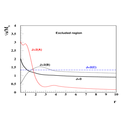
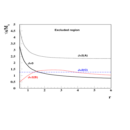
We exhibit in Figs. 3 and 4 the excluded region in the plane $\sqrt{s}/M_{S}\otimes r$ stemming from the requirement that $|\chi_{i}|\leq 1$ and $|{\rm Re}(\chi_{i})|\leq 1/2$ for $n=2$ and 3. As we can see from Fig. 3, the $J=2$ partial wave leads to more stringent bounds than the $J=0$ wave for almost all values of $r$ for $n=2$. Meanwhile, in the case of $n=3$, the $J=0$ partial wave leads to stronger bounds for large $r$. Assuming that the ultraviolet cutoff $r=1$, we find that perturbation theory is valid for $\sqrt{\hat{s}}<M_{S}$. This is what one may naively anticipated. Asymptotically for larger $r$, the limit approaches to $\sqrt{\hat{s}}\leq 0.7M_{S}$ for $n=3$, and $\sqrt{\hat{s}}\leq 0.1M_{S}$ for $n=2$. In the rest of our calculations we make the conservative choice $r=1$ and $\sqrt{\hat{s}}\leq 0.9M_{S}$.

IV Numerical Studies at Hadron Colliders

A Results for Tevatron

Due to the large available center–of–mass energy, the Fermilab Tevatron is a promising facility to look for effects from low scale quantum gravity through diphoton production in hadronic collisions. At Run I, both CDF and DØ studied the production of diphotons [17]. The CDF probed higher $\gamma\gamma$ invariant masses in the range $50<M_{\gamma\gamma}<350$ GeV, but the binning information on the data is not available. It is nevertheless possible to exclude $M_{S}\leq 0.91$ (0.87) TeV for $n=3$ (4) at 95% CL [14].

For Run II there will be a substantial increase in luminosity (2 fb-1) as well as a slightly higher center–of–mass energy (2 TeV). Therefore, we expect to obtain tighter bounds than the ones coming from the Run I. We evaluated the diphoton production cross section imposing that

  • $\bullet$

    $|\eta_{\gamma}|<1$;

  • $\bullet$

    $p_{T}^{\gamma}>12$ GeV;

  • $\bullet$

    $350\hbox{ GeV }<M_{\gamma\gamma}<0.9~{}M_{S}$.

Notice that we introduced a upper bound on $M_{\gamma\gamma}$ in order to guarantee that our perturbative calculation does not violate partial wave unitarity; see Sec. III. The strong cut on the minimal $M_{\gamma\gamma}$ reduces the background from jets faking photons [17] to a negligible level, leaving only the irreducible SM background. After imposing those cuts and assuming a detection efficiency of 80% for each photon, we anticipate 12 reconstructed background events at Run II per experiment.

We display in Fig. 5 the $M_{\gamma\gamma}$ spectrum from the SM and graviton–exchange contributions for $q\bar{q}$ and gluon–gluon fusions. We use in our calculation the MRSG distribution functions [18] and took the $M_{\gamma\gamma}$ as the QCD scales. As we can see from this figure, the $q\bar{q}$ fusion dominates both the SM and graviton contributions and the graviton exchange is the most important source of diphoton at large $\gamma\gamma$ invariant masses. This behavior lead us to introduce the above minimum $M_{\gamma\gamma}$ cut to enhance the signal.

We obtained the $2\sigma$ limits for the quantum gravity scale $M_{S}$ requiring that

$$\frac{\sigma_{tot}-\sigma_{sm}}{\sqrt{\sigma_{sm}}}\sqrt{{\cal L}}\;\epsilon\geq 2\;,$$ (33)

where $\epsilon=0.80$ is the reconstruction efficiency for one photon, $\sigma_{sm}$ is the SM cross section, and $\sigma_{tot}$ the total cross section including the new physics; see Sec. II. We present in Table I the $2\sigma$ attainable bounds on $M_{S}$ at Run II for several choices of $n$ and an integrated luminosity of ${\cal L}=2$ fb-1, corresponding to the observation of 19 events for SM plus signal. Notice that the bounds are better than the ones for Run I [14] because the higher luminosity allows us to perform a more stringent cut on the minimum $M_{\gamma\gamma}$, consequently enhancing the graviton exchange contribution. Furthermore, these bounds do not scale as $(n-2)M_{S}^{4}$ as expected from Eq. (11), showing the importance to take into account the full expression for the graviton propagator.

In order to establish further evidence of the signal from low scale quantum gravity after a deviation from the SM is observed, we study several kinematical distributions, comparing the predictions of the SM and the quantum graviton exchange. We show in Fig. 6 the photon rapidity distributions after the invariant mass and transverse momentum cuts, relaxing the rapidity to be $|\eta_{\gamma}|<3$, for the SM and for the $n=3$ gravity signal with $M_{S}=1.9$ TeV, which corresponds to the $2\sigma$ limit, and $M_{S}=1$ TeV, which leads to a larger anomalous contribution. As we expected, the $s$–channel KK exchange gives rise to more events at low rapidities in comparison with the $t$ and $u$–channel SM background, indicating that an angular distribution study could be crucial to separate the signal from the background. As remarked above, the rapid growth of the $M_{\gamma\gamma}$ spectrum is an important feature for KK graviton exchange; see Fig. 7.

B Results for LHC

The CERN Large Hadron Collider (LHC) will be able to considerably extend the search for low–energy quantum gravity due to its large center–of–mass energy ($\sqrt{s}=14$ TeV) and high luminosity (${\cal L}=10$ $100$ fb-1). Therefore, we have also analyzed the diphoton production at LHC in order to access its potentiality to probe $M_{S}$ via this reaction.

At the LHC there will be a very large gluon–gluon luminosity which will enhance the importance of $gg\to\gamma\gamma$ subprocess, as can be seen from Fig. 8. Therefore, we can anticipate that the interference between the SM loop contribution to this process and the KK graviton exchange will play an important rôle in determining the limits for $M_{S}$ since it is comparable to the leading $q\bar{q}$ anomalous contribution for large $M_{S}$.

At high $\gamma\gamma$ center–of–mass energies the main background is the irreducible SM diphoton production. In order to suppress this background and enhance the signal we applied the following cuts:

  • $\bullet$

    we required the photons to be produced in the central region of the detector, i.e. the polar angle of the photons in the laboratory should satisfy $|\cos\theta_{\gamma}|<0.8$;

  • $\bullet$

    $M_{\gamma\gamma}>0.8~{}(1)$ TeV, according with the luminosity ${\cal L}=10~{}(100)\;{\rm pb}^{-1}$, in order to use the fast decrease of the SM background with the increase of the subprocess center–of–mass energy;

  • $\bullet$

    $M_{\gamma\gamma}<0.9~{}M_{S}$ to be sure that partial wave unitarity is not violated.

The SM contribution after cuts has a cross section of 1.86 (0.83) fb, which corresponds to 18 (83) reconstructed events for ${\cal L}=10~{}(100)$ fb-1.

In Table II, we present the $2\sigma$ attainable limits on $M_{S}$ for different number of extra dimensions and two integrated luminosities ${\cal L}=10$ fb-1 and $100$ fb-1, corresponding to the observation of 27 and 101 events for the SM plus signal respectively. In our calculation we applied the above cuts and used the MRSG parton distribution functions with the renormalization and factorization scales taken to be $M_{\gamma\gamma}$. As we expected, the LHC will be able to improve the Tevatron bounds by a factor $\simeq 4$ due to its higher energy and luminosities. Moreover, our results are slightly better than the other limits presented so far in the literature [9, 10, 11].

In order to learn more about the KK states giving rise to the signal, we should also study characteristic kinematical distributions. For instance, the rapidity distributions due to graviton exchange are distinct from the SM one since the signal contribution takes place via $s$–channel exchanges while the backgrounds are $u$– and $t$–channel processes. We show in Fig. 9 the photon rapidity spectrum after the invariant mass cut and requiring that $|\eta_{\gamma}|<3$, including the signal for $M_{S}=6.7$ TeV and $M_{S}=3$ TeV with $n=3$ and the SM backgrounds. As expected, the distribution for the graviton signal is more central than the background. Analogously to the Tevatron analysis, the KK modes also show themselves in the high diphoton invariant mass region as seen in Fig. 10.

V Discussion and Conclusions

High center–of–mass energies at hadron colliders provide a good opportunity to probe the physics with low–scale quantum gravity. We have analyzed the potentiality of hadron colliders to search for large extra dimensions signals via the production of photon pairs. Although the virtual exchange of Kaluza–Klein gravitons may significantly enhance the rate for this processes and presents characteristically different kinematical distributions from the SM process, it is sensitive to an unknown ultraviolet cutoff $\Lambda$, which should be at ${\cal O}(M_{S})$. We examined the constraints on the relation between $\sqrt{s}$ and $M_{S}$ from the partial wave unitarity as a function of this cutoff. Keeping in mind the unitarity constraint, we calculated in detail the subprocesses $q\bar{q}\to\gamma\gamma$ and $gg\to\gamma\gamma$ taking into account the complete Standard Model and graviton contributions. We found that the Tevatron is able to probe $M_{S}$ at the 2$\sigma$ level up to 1.5–1.9 TeV at Run II, for 7–3 extra dimensions; while the LHC can extend this search to 5.3 (6.5)–6.7 (8.5) TeV for a luminosity ${\cal L}=10$ $(100)$ fb-1.

It is important to notice that our results are better, or at least comparable, to the ones presented in the literature so far. At the Tevatron, it is already clear that the Run II will provide stronger limits on the new graviton scale due simply to the enhancement of the luminosity. Our analysis shows that a careful kinematical study for the diphoton production would improve the limits obtained so far in the Run II from other process as Drell-Yan production [9], $p\bar{p}\rightarrow\hbox{jet}+E\!\!\!\!/\;$ [10] and top production [11]. In the LHC, besides the kinematical cuts suggested here, the inclusion of the SM box diagrams for $gg\rightarrow\gamma\gamma$ also improves the signal, since its contribution in the interference level is no longer negligible. As a matter of fact, our results are comparable to the best ones presented so far, obtained from the process $p\bar{p}\rightarrow\hbox{jet}+E\!\!\!\!/\;$ by Giudice et. al. [10].

Acknowledgements.
This research was supported in part by the University of Wisconsin Research Committee with funds granted by the Wisconsin Alumni Research Foundation, by the U.S. Department of Energy under grant DE-FG02-95ER40896 and DE-FG03-94ER40833, by Conselho Nacional de Desenvolvimento Científico e Tecnológico (CNPq), by Fundação de Amparo à Pesquisa do Estado de São Paulo (FAPESP), and by Programa de Apoio a Núcleos de Excelência (PRONEX).
Note added: When we were preparing this manuscript we became aware of Ref. [19] which also studies the diphoton production at the LHC.

A Helicity Amplitudes for the Box Diagrams

The independent helicity amplitudes for the SM process $gg\to\gamma\gamma$ including only the contribution of a massless quark are

$\displaystyle{\cal M}^{++++}_{sm}(s,t,u)$ $\displaystyle=$ $\displaystyle-i~{}\delta_{ab}~{}8Q_{q}^{2}\alpha\alpha_{s}~{}\left\{1+\frac{u-t}{s}\ln\left(\frac{u}{t}\right)+\frac{1}{2}\frac{t^{2}+u^{2}}{s^{2}}\left[\ln^{2}\left(\frac{u}{t}\right)+\pi^{2}\right]\right\}\;;$ (A1)
$\displaystyle{\cal M}^{++--}_{sm}(s,t,u)$ $\displaystyle=$ $\displaystyle i~{}\delta_{ab}~{}8Q_{q}^{2}\alpha\alpha_{s}\;;$ (A2)
$\displaystyle{\cal M}^{++-+}_{sm}(s,t,u)$ $\displaystyle=$ $\displaystyle-i~{}\delta_{ab}~{}8Q_{q}^{2}\alpha\alpha_{s}\;;$ (A3)

with $\alpha_{s}$ being the strong coupling constant, $Q_{q}$ the quark charge, $a$ and $b$ standing for the gluon colors, and $s$, $t$ and $u$ the Mandelstam invariants. The remaining helicity amplitudes can be obtained from the above expressions through parity and crossing relations [20]:

$\displaystyle{\cal M}^{\pm\pm\mp\pm}(s,t,u)$ $\displaystyle=$ $\displaystyle{\cal M}^{\pm\mp\pm\pm}(s,t,u)={\cal M}^{\pm\mp\mp\mp}(s,t,u)={\cal M}^{\pm\pm\pm\mp}(s,t,u)\;;$ (A4)
$\displaystyle{\cal M}^{--++}(s,t,u)$ $\displaystyle=$ $\displaystyle{\cal M}^{++--}(s,t,u)\;;$ (A5)
$\displaystyle{\cal M}^{\pm\mp\pm\mp}(s,t,u)$ $\displaystyle=$ $\displaystyle{\cal M}^{----}(u,t,s)={\cal M}^{++++}(u,t,s)\;;$ (A6)
$\displaystyle{\cal M}^{\pm\mp\mp\pm}(s,t,u)$ $\displaystyle=$ $\displaystyle{\cal M}^{++++}(t,u,s)\;.$ (A7)

On the other hand, the top contribution is given by

$\displaystyle{\cal M}^{++++}_{sm}(s,t,u)$ $\displaystyle=$ $\displaystyle\frac{i}{2}\delta_{ab}8Q_{q}^{2}\alpha\alpha_{s}\left\{-2+\frac{1}{s^{2}}\left[2(u^{2}-t^{2})(B_{0}(t)-B_{0}(u))+(C_{0}(t)t+C_{0}(u)u)\times\right.\right.$ (A8)
$\displaystyle\times$ $\displaystyle(8m_{t}^{2}s-2t^{2}-2u^{2})+(D_{0}(s,t)+D_{0}(s,u))s^{2}m_{t}^{2}(-4m_{t}^{2}+2s)+$ (A9)
$\displaystyle+$ $\displaystyle\left.\left.D_{0}(t,u)\left(-4m_{t}^{4}s^{2}+2m_{t}^{2}st^{2}-4m_{t}^{2}stu+t^{3}u+2m_{t}^{2}su^{2}+tu^{3}\right)\right]\right\}\;\;;$ (A10)
$\displaystyle{\cal M}^{++--}_{sm}(s,t,u)$ $\displaystyle=$ $\displaystyle i\delta_{ab}8Q_{q}^{2}\alpha\alpha_{s}\left[1-2m_{t}^{4}\left(D_{0}(s,t)+D_{0}(s,u)+D_{O}(t,u)\right)\right]\;\;;$ (A11)
$\displaystyle{\cal M}^{++-+}_{sm}(s,t,u)$ $\displaystyle=$ $\displaystyle i\delta_{ab}8Q_{q}^{2}\alpha\alpha_{s}\left\{-1+\frac{1}{stu}\left[2m_{t}^{2}\left(C_{0}(s)s+C_{0}(t)t+C_{0}(u)u\right)\left(t^{2}+tu+u^{2}\right)+\right.\right.$ (A12)
$\displaystyle+$ $\displaystyle 2m_{t}^{4}stu\left(D_{0}(s,t)+D_{0}(s,u)+D_{0}(t,u)\right)+m_{t}^{2}s^{2}t^{2}D_{0}(s,t)+$ (A13)
$\displaystyle+$ $\displaystyle\left.\left.m_{t}^{2}s^{2}u^{2}D_{0}(s,u)+m_{t}^{2}t^{2}u^{2}D_{0}(t,u)\right]\right\}\;\;,$ (A14)

where $m_{t}$ is the top quark mass and $B_{0}$, $C_{0}$ and $D_{0}$ are Passarino–Veltman functions [21]

$\displaystyle B_{0}(s)$ $\displaystyle\equiv$ $\displaystyle B_{0}(s,m_{t},m_{t})\;\;;$ (A15)
$\displaystyle C_{0}(s)$ $\displaystyle\equiv$ $\displaystyle C_{0}(0,0,s,m_{t},m_{t},m_{t})\;\;;$ (A16)
$\displaystyle D_{0}(s,t)$ $\displaystyle\equiv$ $\displaystyle D_{0}(0,0,0,0,s,t,m_{t},m_{t},m_{t},m_{t})\;\;.$ (A17)

REFERENCES

  • [1] See, for instance, M. B. Green, J. H. Schwarz, and E. Witten, Superstring Theory, Cambridge Press (1987).
  • [2] N. Arkani–Hamed, S. Dimopoulos, and G. Dvali, Phys. Lett. B429, 263 (1998); I. Antoniadis, N. Arkani-Hamed, S. Dimopoulos, and G. Dvali, Phys. Lett. B436, 257 (1998); I. Antoniadis and C. Bachas, Phys. Lett. B450, 83 (1999).
  • [3] N. Arkani–Hamed, S. Dimopoulos, and G. Dvali, Phys. Rev. D59, 086004 (1999).
  • [4] S. Cullen and M. Perelstein, hep-ph/9903422; V. Barger, T. Han, C. Kao, and R. Zhang, hep-ph/9905474.
  • [5] See, e. g., Modern Kaluza-Klein Theories, eds. T. Appelquist, A. Chodos and P. Freund, Addison-Wesley Pub. (1987).
  • [6] E. Witten, Nucl. Phys. B443, 85 (1995); P. Hořava and E. Witten, Nucl. Phys. B460, 506 (1996); Nucl. Phys. B475, 94 (1996).
  • [7] For recent discussions, see for example, C. Efthimiou and B. Greene (Ed.), TASI96: Fields, Strings and Duality, World Scientific, Singapore (1997) and references therein.
  • [8] I. Antoniadis, Phys. Lett. B246, 377 (1990); J. Lykken, Phys. Rev. D54, 3693 (1996); K. Dienes, E. Dudas, and T. Ghergetta, Phys. Lett. B436, 55 (1998). G. Shiu and S.-H. H. Tye, Phys. Rev. D58, 106007 (1998); Z. Kakushadze and S.-H. H. Tye, Nucl. Phys. B548, 180 (1999); L. E. Ibáñez, C. Muñoz and S. Rigolin, hep-ph/9812397.
  • [9] J. Hewett, Phys. Rev. Lett. 82, 4765 (1999).
  • [10] G. F. Giudice, R. Rattazzi and J. D. Wells, Nucl. Phys. B544, 3 (1999); E. A. Mirabelli, M. Perelstein and M. E. Peskin, Phys. Rev. Lett. 82, 2236 (1999).
  • [11] P. Mathews, S. Raychaudhuri, and K. Sridhar, Phys. Lett. B450, 343 (1999); T. Rizzo, hep-ph/9902273.
  • [12] T. Han, J. Lykken, and Ren–Jie Zhang, Phys. Rev. D59, 105006 (1999).
  • [13] A. K. Gupta, N. K. Mondal, and S. Raychaudhuri, hep-ph/9904234; P. Mathews, S. Raychaudhuri, and K. Sridhar, Phys. Lett. B455, 115 (1999) and hep-ph/9904232; T. Rizzo, Phys. Rev. D59, 115010 (1999), hep-ph/9903475 and hep-ph/9904380; S.Y. Choi et al., Phys. Rev. D60, 013007 (1999); K. Agashe and N.G. Deshpande, Phys. Lett. B456, 60 (1999); K. Cheung and W.-Y. Keung, hep-ph/9903294; D. Atwood, S. Bar-Shalom, and A. Soni, hep-ph/9903538; C. Balazs et al., hep-ph/9904220; G. Shiu, R. Shrock, and S.-H. H. Tye, hep-ph/9904262; K. Y. Lee, H.S. Song, and J. Song, hep-ph/9904355; Hooman Davoudiasl, hep-ph/9904425; K. Cheung, hep-ph/9904510; T. Han, D. Rainwater, and D. Zeppenfeld, hep-ph/9905423; Xiao-Gang He, hep-ph/9905500.
  • [14] K. Cheung, hep-ph/9904266.
  • [15] V. Constantini, B. de Tollis, and G. Pistoni, Nuovo Cimento 2A, 733 (1971); Ll. Ametler, et al., Phys. Rev. D32, 1699 (1985); D. Dicus and S Willenbrock, Phys. Rev. D37, 1801 (1988).
  • [16] Particle Data Group, Eur. Phys. J. C3, 1 (1998).
  • [17] F. Abe et al., CDF Collaboration, Phys. Rev. D59, 092002 (1999); “Searching for Higgs Mass Photon Pair in $p\bar{p}$ Collitions at $\sqrt{s}=1.8$ TeV”, submitted by P. Wilson (CDF Collaboration) to ICHEP’98; “Direct Photon Measurements at D0”, submitted by D0 Collaboration to ICHEP’98.
  • [18] A. D. Martin, R. G. Roberts, and W. J. Stirling, Phys. Lett. B354, 155 (1995).
  • [19] D. Atwood, S. Bar-Shalom, and A. Soni, hep-ph/9906400.
  • [20] G. Jikia and A. Tkabladze, Phys. Lett. B323, 453 (1994).
  • [21] G. Passarino and M. Veltman, Nucl. Phys. B160, 151 (1979).
$n$ 3 4 5 6 7
$M_{S}$ (TeV) 1.92 1.73 1.61 1.52 1.45

TABLE I.: $2\sigma$ limits in TeV for the quantum gravity scale $M_{S}$ as a function of the number of extra dimensions for the Tevatron Run II.
$n$ 3 4 5 6 7
${\cal L}=10$ fb-1 6.70 6.15 5.78 5.50 5.28
${\cal L}=100$ fb-1 8.50 7.70 7.16 6.79 6.50

TABLE II.: $2\sigma$ limits in TeV for the extra dimensions gravity scale $M_{S}$ as a function of the number of extra dimensions for the LHC with luminosities ${\cal L}=10$ and $100$ fb-1.

\ArrowLine(0,20)(40,20) \ArrowLine(40,60)(0,60) \ArrowLine(40,20)(40,60) \Photon(40,20)(80,20)43 \Photon(40,60)(80,60)43 \Text(20,10)[c]$q$\Text(20,70)[c]$\bar{q}$\Text(35,40)[r]$q$\Text(85,20)[l]$\gamma(k^{\prime})$\Text(85,60)[l]$\gamma(k)$\ArrowLine(150,20)(190,20) \ArrowLine(190,60)(150,60) \ArrowLine(190,20)(190,60) \Photon(190,20)(230,60)44 \Photon(190,60)(230,20)44 \Text(170,10)[c]$q$\Text(170,70)[c]$\bar{q}$\Text(185,40)[r]$q$\Text(235,20)[l]$\gamma(k^{\prime})$\Text(235,60)[l]$\gamma(k)$\ArrowLine(300,20)(330,40) \ArrowLine(330,40)(300,60) \Photon(330,40)(360,40)45 \Photon(360,40)(330,40)-45 \Photon(360,40)(390,20)43 \Photon(360,40)(390,60)-43 \Text(300,20)[r]$q$\Text(300,60)[r]$\bar{q}$\Text(345,50)[c]$KK$\Text(395,20)[l]$\gamma(k^{\prime})$\Text(395,60)[l]$\gamma(k)$

FIG. 1.: Feynman diagrams contributing to the subprocess $q\bar{q}\to\gamma\gamma$, including the Kaluza–Klein graviton exchange.

\Gluon(10,20)(50,20)-44 \Gluon(10,60)(50,60)-44 \ArrowLine(50,20)(50,60) \ArrowLine(50,60)(90,60) \ArrowLine(90,60)(90,20) \ArrowLine(90,20)(50,20) \Photon(90,20)(130,20)43 \Photon(90,60)(130,60)43 \Text(5,20)[r]$g$\Text(5,60)[r]$g$\Text(45,40)[r]$q$\Text(70,70)[c]$q$\Text(95,40)[l]$q$\Text(70,10)[c]$q$\Text(135,20)[l]$\gamma(k^{\prime})$\Text(135,60)[l]$\gamma(k)$\Gluon(200,10)(240,40)-44 \Gluon(200,70)(240,40)44 \Photon(240,40)(280,40)45 \Photon(240,40)(280,40)-45 \Photon(280,40)(320,10)43 \Photon(280,40)(320,70)-43 \Text(195,10)[r]$g$\Text(195,70)[r]$g$\Text(260,50)[c]$KK$\Text(325,10)[l]$\gamma(k^{\prime})$\Text(325,70)[l]$\gamma(k)$

FIG. 2.: Feynman diagrams contributing to the subprocess $gg\to\gamma\gamma$, including the Kaluza–Klein graviton exchange. The crossed diagrams are not displayed.
Refer to caption
FIG. 3.: $J=0$ and 2 unitarity bounds in the plane $\sqrt{s}/M_{S}\otimes r$ for the elastic $\gamma\gamma$ scattering and $n=2$. $J=2$(A) corresponds to the limit from the eigenvalue $\chi=|a^{2}_{0;0}|<1$, (B) to $2|a^{2}_{2;2}|<1$ and (C) to $2|Re(a^{2}_{2;2})|<1/2$.
Refer to caption
FIG. 4.: Same as in Fig. 3 but for $n=3$.
Refer to caption
FIG. 5.: $\gamma\gamma$ spectrum originated from the SM (solid lines) and graviton–exchange (dashed) contributions for $q\bar{q}$ and gluon–gluon fusions at the Tevatron Run II. In this figure we took $M_{S}=1$ TeV, $n=3$, and applied the cuts described in the text, using now $M_{\gamma\gamma}>150$ GeV.
Refer to caption
FIG. 6.: Rapidity distributions of the photons for the SM background (solid line) and for the signal for $M_{S}=1.9$ TeV (dashed line) and $M_{S}=1$ TeV (dotted line) with $n=3$ at the Tevatron Run II. We imposed the cuts $|\eta_{\gamma}|<3$, $350$ GeV $<M_{\gamma\gamma}<0.9M_{S}$ and $p_{T}^{\gamma}>12$ GeV.
Refer to caption
FIG. 7.: Invariant mass distributions of the photon pair for the SM background (solid line) and for the signal for $M_{S}=1.9$ TeV (dashed line) and $M_{S}=1$ TeV (dot-dashed line) with $n=3$ at the Tevatron Run II. We imposed the cuts $|\eta_{\gamma}|<1$, $150$ GeV $<M_{\gamma\gamma}<0.9M_{S}$ and $p_{T}^{\gamma}>12$ GeV.
Refer to caption
FIG. 8.: $\gamma\gamma$ spectrum originated from the SM (solid lines) and graviton–exchange (dashed) contributions for $q\bar{q}$ and gluon–gluon fusions at the LHC. We took $M_{S}=4.7$ TeV, $n=3$, and applied the cuts described in the text, using now $M_{\gamma\gamma}>400$ GeV.
Refer to caption
FIG. 9.: Rapidity distributions of the photons for the SM background (solid line) and for the signal for $M_{S}=6.7$ TeV (dashed line) and $M_{S}=3$ TeV (dotted line) with $n=3$ at the LHC. We imposed the cuts $|\eta_{\gamma}|<3$ and $800$ GeV $<M_{\gamma\gamma}<0.9M_{S}$.
Refer to caption
FIG. 10.: Invariant mass distributions of the photon pair for the SM background (solid line) and the signal for $M_{S}=6.7$ TeV (dashed line) and $M_{S}=3$ TeV (dot–dashed line) with $n=3$ at the LHC. We imposed the angular cut $|\cos\theta_{\gamma}|<0.8$ and $400$ GeV $<M_{\gamma\gamma}<0.9M_{S}$.