Pauli–Villars regularization in DLCQ

Abstract

Calculations in a (3+1)-dimensional model indicate that Pauli-Villars regularization can be combined with discrete light-cone quantization (DLCQ) to solve at least some field theories nonperturbatively. Discrete momentum states of Pauli-Villars particles are included in the Fock basis to automatically generate needed counterterms; the resultant increase in basis size is found acceptable. The Lanczos algorithm is used to extract the lowest massive eigenstate and eigenvalue of the light-cone Hamiltonian, with basis sizes ranging up to 10.5 million. Each Fock-sector wave function is computed in this way, and from these one can obtain values for various quantities, such as average multiplicities and average momenta of constituents, structure functions, and a form-factor slope.

Introduction

Field-theoretic calculations of bound-state properties, such as those one would like to do for quantum chromodynamics (QCD), require regularization of infinities and renormalization of parameters. As a way of providing a systematic regularization of ultraviolet infinities we study PV1 ; PV2 the use of Pauli–Villars (PV) regularization PauliVillars in the context of discrete light-cone quantization (DLCQ) PauliBrodsky ; DLCQreview . Renormalization is accomplished by adjusting bare parameters to fit selected state properties with “data.” The problem to be solved is then a bound-state eigenvalue problem, which includes PV constituents, combined with renormalization conditions. The couplings of the PV constituents are chosen to produce desired cancellations in perturbation theory.

We have tested these ideas for two related (3+1)-dimensional Hamiltonians PV1 ; PV2 . The first PV1 was constructed to have an analytic solution, in analogy with the equal-time model of Greenberg and Schweber GreenbergSchweber . The second Hamiltonian PV2 is a generalization of the first which assigns proper light-cone energies to all particles, but does not have an analytic solution. Both Hamiltonians are distantly related to Yukawa theory, in that a fermion field acts as a source and sink for bosons. The second Hamiltonian and some of the results obtained will be described here. Work on direct application to Yukawa theory is in progress.

The choice of light-cone coordinates ($x^{\pm}=t\pm z$, $\bf{x}_{\perp}=(x,y)$) Dirac ; DLCQreview is driven by important advantages, which include kinematical boosts, a simple vacuum, and well-defined Fock-state expansions with no disconnected pieces. The latter two derive from the positivity of the longitudinal light-cone momentum $p^{+}=E+p_{z}$. When momenta are discretized PauliBrodsky this positivity brings the additional advantage of a finite limit on the number of constituents.

Model Eigenvalue Problem

The bound-state eigenvalue problem is $H_{\rm LC}\Phi_{\sigma}=M^{2}\Phi_{\sigma}$, where $H_{\rm LC}=P^{+}P^{-}$ is known as the light-cone Hamiltonian, $P^{+}$ is the longitudinal momentum operator, and $P^{-}$ is the generator for evolution in light-cone time. We work in the frame with no net transverse momentum and in a basis diagonal in $P^{+}$.

The Hamiltonian that we consider is

$$H_{\rm LC} = \int\frac{dp^{+}d^{2}p_{\perp}}{16\pi^{3}p^{+}}(\frac{M^{2}+p_{\perp}^{2}}{p^{+}/P^{+}}+M^{\prime}_{0}p^{+}/P^{+})\sum_{\sigma}b_{\underline{p}\sigma}^{\dagger}b_{\underline{p}\sigma}$$

$$+\int\frac{dq^{+}d^{2}q_{\perp}}{16\pi^{3}q^{+}}\left[\frac{\mu^{2}+q_{\perp}^{2}}{q^{+}/P^{+}}a_{\underline{q}}^{\dagger}a_{\underline{q}}+\frac{\mu_{1}^{2}+q_{\perp}^{2}}{q^{+}/P^{+}}a_{1\underline{q}}^{\dagger}a_{1\underline{q}}\right]$$

$$+g\int\frac{dp_{1}^{+}d^{2}p_{\perp 1}}{\sqrt{16\pi^{3}p_{1}^{+}}}\int\frac{dp_{2}^{+}d^{2}p_{\perp 2}}{\sqrt{16\pi^{3}p_{2}^{+}}}\int\frac{dq^{+}d^{2}q_{\perp}}{16\pi^{3}q^{+}}\sum_{\sigma}b_{\underline{p}_{1}\sigma}^{\dagger}b_{\underline{p}_{2}\sigma}$$

$$\rule{18.06749pt}{0.0pt}\times\left[a_{\underline{q}}^{\dagger}\delta(\underline{p}_{1}-\underline{p}_{2}+\underline{q})+a_{\underline{q}}\delta(\underline{p}_{1}-\underline{p}_{2}-\underline{q})\right.$$

$$\rule{36.135pt}{0.0pt}\left.+ia_{1\underline{q}}^{\dagger}\delta(\underline{p}_{1}-\underline{p}_{2}+\underline{q})+ia_{1\underline{q}}\delta(\underline{p}_{1}-\underline{p}_{2}-\underline{q})\right]\,.$$

The creation operators $b_{\underline{p}\sigma}^{\dagger}$, $a_{\underline{q}}^{\dagger}$, and $a_{1\underline{q}}^{\dagger}$ are associated with fermion, boson, and PV boson fields, respectively. The corresponding masses are $M$, $\mu$, and $\mu_{1}$. Each operator depends on a light-cone three-momentum such as $\underline{p}\equiv(p^{+},p_{x},p_{y})$. The nonzero commutation relations are

$$\left\{b_{\underline{p}\sigma},b_{\underline{p}^{\prime}\sigma^{\prime}}^{\dagger}\right\} = 16\pi^{3}p^{+}\delta(\underline{p}-\underline{p}^{\prime})\delta_{\sigma\sigma^{\prime}}\,,$$ (2)

$$\left[a_{\underline{q}},a_{\underline{q}^{\prime}}^{\dagger}\right] = 16\pi^{3}q^{+}\delta(\underline{q}-\underline{q}^{\prime})\,,\;\;\left[a_{1\underline{q}},a_{1\underline{q}^{\prime}}^{\dagger}\right]=16\pi^{3}q^{+}\delta(\underline{q}-\underline{q}^{\prime})\,.$$

The structure of the Hamiltonian provides for emission and absorption of bosons by the fermion, but no change in fermion number. We explore only the one-fermion sector. The particular form of the interaction causes the fermion mass counterterm to have an unusual momentum dependence. The coefficient of this counterterm is finite because of cancellations arranged by assigning an imaginary coupling to the PV boson.

The state vector $\Phi_{\sigma}$ describes a dressed fermion with spin $\sigma$. Its Fock-state expansion is given by

$$\Phi_{\sigma} = \sqrt{16\pi^{3}P^{+}}\sum_{n,n_{1}}\int\frac{dp^{+}d^{2}p_{\perp}}{\sqrt{16\pi^{3}p^{+}}}\prod_{i=1}^{n}\int\frac{dq_{i}^{+}d^{2}q_{\perp i}}{\sqrt{16\pi^{3}q_{i}^{+}}}\prod_{j=1}^{n_{1}}\int\frac{dr_{j}^{+}d^{2}r_{\perp j}}{\sqrt{16\pi^{3}r_{j}^{+}}}$$

$$\times\delta(\underline{P}-\underline{p}-\sum_{i}^{n}\underline{q}_{i}-\sum_{j}^{n_{1}}\underline{r}_{j})\phi^{(n,n_{1})}(\underline{q}_{i},\underline{r}_{j};\underline{p})\frac{1}{\sqrt{n!n_{1}!}}b_{\underline{p}\sigma}^{\dagger}\prod_{i}^{n}a_{\underline{q}_{i}}^{\dagger}\prod_{j}^{n_{1}}a_{1\underline{r}_{j}}^{\dagger}|0\rangle\,,$$

with normalization $\Phi_{\sigma}^{\prime\dagger}\cdot\Phi_{\sigma}=16\pi^{3}P^{+}\delta(\underline{P}^{\prime}-\underline{P})$, which implies

$$1=\sum_{n,n_{1}}\prod_{i}^{n}\int\,dq_{i}^{+}d^{2}q_{\perp i}\prod_{j}^{n_{1}}\int\,dr_{j}^{+}d^{2}r_{\perp j}\left|\phi^{(n,n_{1})}(\underline{q}_{i},\underline{r}_{j};\underline{P}-\sum_{i}\underline{q}_{i}-\sum_{j}\underline{r}_{j})\right|^{2}\,.$$ (4)

To satisfy the eigenvalue condition, the Fock-sector wave functions $\phi^{(n,n_{1})}$ must solve the following coupled system:

$$\left[M^{2}-\frac{M^{2}+p_{\perp}^{2}}{p^{+}/P^{+}}-M^{\prime}_{0}p^{+}/P^{+}-\sum_{i}\frac{\mu^{2}+q_{\perp i}^{2}}{q_{i}^{+}/P^{+}}-\sum_{j}\frac{\mu_{1}^{2}+r_{\perp j}^{2}}{r_{j}/P^{+}}\right]\phi^{(n,n_{1})}(\underline{q}_{i},\underline{r}_{j},\underline{p})$$

$$=g\left\{\sqrt{n+1}\int\frac{dq^{+}d^{2}q_{\perp}}{\sqrt{16\pi^{3}q^{+}}}\phi^{(n+1,n_{1})}(\underline{q}_{i},\underline{q},\underline{r}_{j},\underline{p}-\underline{q})\right.$$

$$\rule{36.135pt}{0.0pt}+\frac{1}{\sqrt{n}}\sum_{i}\frac{1}{\sqrt{16\pi^{3}q_{i}^{+}}}\phi^{(n-1,n_{1})}(\underline{q}_{1},\ldots,\underline{q}_{i-1},\underline{q}_{i+1},\ldots,\underline{q}_{n},\underline{r}_{j},\underline{p}+\underline{q}_{i})$$

$$\rule{36.135pt}{0.0pt}+i\sqrt{n_{1}+1}\int\frac{dr^{+}d^{2}r_{\perp}}{\sqrt{16\pi^{3}r^{+}}}\phi^{(n,n_{1}+1)}(\underline{q}_{i},\underline{r}_{j},\underline{r},\underline{p}-\underline{r})$$

$$\rule{36.135pt}{0.0pt}+\left.\frac{i}{\sqrt{n_{1}}}\sum_{j}\frac{1}{\sqrt{16\pi^{3}r_{j}^{+}}}\phi^{(n,n_{1}-1)}(\underline{q}_{i},\underline{r}_{1},\ldots,\underline{r}_{j-1},\underline{r}_{j+1},\ldots,\underline{r}_{n_{1}},\underline{p}+\underline{r}_{j})\right\}\,.$$

The bare parameters $M^{\prime}_{0}$ and $g$ are determined by fitting $\langle:\!\!\phi^{2}(0)\!\!:\rangle\equiv\Phi_{\sigma}^{\dagger}\!:\!\!\phi^{2}(0)\!\!:\!\Phi_{\sigma}$ and $M^{2}$ to chosen values. The quantity $\langle:\!\!\phi^{2}(0)\!\!:\rangle$ was selected for ease of computation; it can be computed from a form similar to the normalization sum (4):

$$\langle:\!\!\phi^{2}(0)\!\!:\rangle = \sum_{n=1,n_{1}=0}\prod_{i}^{n}\int\,dq_{i}^{+}d^{2}q_{\perp i}\prod_{j}^{n_{1}}\int\,dr_{j}^{+}d^{2}r_{\perp j}$$

$$\rule{18.06749pt}{0.0pt}\times\left(\sum_{k=1}^{n}\frac{2}{q_{k}^{+}/P^{+}}\right)\left|\phi^{(n,n_{1})}(\underline{q}_{i},\underline{r}_{j};\underline{P}-\sum_{i}\underline{q}_{i}-\sum_{j}\underline{r}_{j})\right|^{2}\,.$$

The renormalization conditions that determine $M^{\prime}_{0}$ and $g$ are then solved simultaneously with the eigenvalue problem (Model Eigenvalue Problem). In practice this is done by rearranging (Model Eigenvalue Problem) into an eigenvalue problem for $1/g$ and simultaneously solving for $M^{\prime}_{0}$ in a single nonlinear equation where $\langle:\!\!\phi^{2}(0)\!\!:\rangle$ is equal to a fixed value. The simultaneous solution is done by iterative means.

Once the wave functions $\phi^{(n,n_{1})}$ have been obtained, they can be used to compute various quantities, such as the boson structure function

$$f_{B}(y) \equiv \sum_{n,n_{1}}\prod_{i}^{n}\int\,dq_{i}^{+}d^{2}q_{\perp i}\prod_{j}^{n_{1}}\int\,dr_{j}^{+}d^{2}r_{\perp j}\sum_{i=1}^{n}\delta(y-q_{i}^{+}/P^{+})$$

$$\rule{36.135pt}{0.0pt}\times\left|\phi^{(n,n_{1})}(\underline{q}_{i},\underline{r}_{j};\underline{P}-\sum_{i}\underline{q}_{i}-\sum_{j}\underline{r}_{j})\right|^{2}$$

and the average boson multiplicity and momentum

$$\langle n_{B}\rangle=\int_{0}^{1}f_{B}(y)dy\,,\;\;\langle y\rangle=\int_{0}^{1}yf_{B}(y)dy\,.$$ (8)

We also compute the slope of the fermion “charge” form factor $F^{\prime}(0)$, from an expression derived in Ref. PV1 .

Numerical methods and results

The coupled equations (Model Eigenvalue Problem) are converted to a finite matrix eigenvalue problem by applying the DLCQ procedure PauliBrodsky . Integrals are approximated by sums over discrete momentum values $(n\pi/L,n_{x}\pi/L_{\perp},n_{y}\pi/L_{\perp})$, and the transverse range is limited by a cutoff $\Lambda^{2}$ such that $(m_{i}^{2}+p_{\perp i})\leq\Lambda^{2}p_{i}^{+}/P^{+}$ for each particle, with $m_{i}$ being its mass. The length scales $L$ and $L_{\perp}$ are associated with a light-cone coordinate box. Bosons are assigned periodic boundary conditions and the fermion is assigned an antiperiodic boundary condition in the longitudinal direction. The momentum integer $n$ is then even for bosons and odd for the fermion.

The total longitudinal momentum $P^{+}$ of the dressed fermion defines an odd integer $K=P^{+}L/\pi$, called the harmonic resolution PauliBrodsky . A longitudinal momentum fraction $x=p^{+}/P^{+}$ then reduces to a rational number $n/K$. The positivity of longitudinal momentum implies that $0<n\leq K$ and that the maximum number of constituents is of order $K/2$. The integers $n_{x}$ and $n_{y}$ range between $-N_{\perp}$ and $N_{\perp}$, with $N_{\perp}$ set to reach the limit imposed by the transverse cutoff for the one-boson physical state.

Thus the discretization is determined by three parameters: $K$, $N_{\perp}$, and $\Lambda^{2}$. The transverse scale $L_{\perp}$ is computed from these as $L_{\perp}=\pi N_{\perp}\sqrt{2/(\Lambda^{2}-M^{2}-\mu^{2})}$. The longitudinal scale does not appear PauliBrodsky , but the limit $L\rightarrow\infty$ is equivalent to $K\rightarrow\infty$. We therefore study the limit where $K$, $N_{\perp}$, and $\Lambda^{2}$ all become large. This recovers the continuum form of the theory, which is regulated by the PV mass $\mu_{1}$, not by $\Lambda$. We must then also study the large $\mu_{1}$ limit.

Typical discretizations, such as $K=15$, $N_{\perp}=6$, and $\Lambda^{2}=50\mu^{2}$, with $\mu_{1}^{2}=10\mu^{2}$ produce matrices with ranks on the order of 5 million. The largest calculations carried out were of rank 10.5 million, which required approximately 2 hours of cpu time on a single 4-processor node of an IBM SP. The diagonalization method used is the Lanczos algorithm for complex symmetric matrices Lanczos .

Although the automatic truncation of particle number imposed by DLCQ can be sufficient, further truncation can be made when the coupling is weak. Such truncation, typically to 4 bosons, was used to permit increased resolution within fixed memory limits. The validity of such an approximation was checked by computing the contribution of individual Fock sectors to the total norm.

Most quantities are remarkably insensitive to numerical resolution. This can be seen in Fig. 1 where we display the boson structure function $f_{B}$ for various mass ratios $M/\mu$. Different values of $K$ and $N_{\perp}$ generally do not yield significantly different results. Notice that a smaller mass ratio is associated with a state where the boson constituents carry more of the momentum.

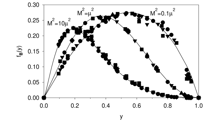
Figure 1: The boson structure function $f_{B}$ at various numerical resolutions and mass values, with $\langle:\!\!\phi^{2}(0)\!\!:\rangle=1$, $\Lambda^{2}=50\mu^{2}$, and $\mu_{1}^{2}=10\mu^{2}$. The solid lines are parameterized fits of the form $Ay^{a}(1-y)^{b}e^{-cy}$.

Values for a set of bound-state observables are given in Table 1. The quantity $|\phi_{0}|^{2}$ represents the probability for the bare fermion state. Each entry has been extrapolated from the numerical results by fits to the form $\alpha+\beta/K^{2}+\gamma/N_{\perp}^{2}$. To obtain the behavior of this form the use of weighting factors PV1 in DLCQ sums is important. The numerical resolutions used ranged from 9 to 19 for $K$ and 5 to as much as 10 for $N_{\perp}$; the larger values of $N_{\perp}$ were available only for smaller $K$. Most observables converge quickly with respect to the PV regulator mass $\mu_{1}$. Only $M^{\prime}_{0}$ is strongly dependent on $\mu_{1}$. The form factor slope is sensitive to the transverse resolution and range.

Table 1: Extrapolated bare parameters and observables, with $\langle:\!\!\phi^{2}(0)\!\!:\rangle=1$.

$(M/\mu)^{2}$	1	1	1	1	1	1	1	0.1	5	10
$(\mu_{1}/\mu)^{2}$	5	5	5	10	10	20	20	10	10	10
$(\Lambda/\mu)^{2}$	12.5	25	50	25	50	50	100	50	100	100
$g/\mu$	21.4	17.7	16.3	17.8	16.0	16.0	15.5	15.1	18.1	19.0
$M^{\prime}_{0}/\mu^{2}$	1.26	1.10	1.10	1.48	1.4	1.8	1.9	1.39	1.66	1.60
$|\phi_{0}|^{2}$	0.82	0.83	0.84	0.85	0.86	0.87	0.87	0.83	0.89	0.90
$-100\mu^{2}F^{\prime}(0)$	1.04	0.78	0.66	0.72	0.59	0.59	0.51	2.0	0.14	0.07
$\langle n_{B}\rangle$	0.18	0.15	0.14	0.15	0.14	0.13	0.13	0.16	0.10	0.09
$\langle y\rangle$	0.077	0.062	0.057	0.062	0.056	0.056	0.053	0.073	0.032	0.024

Summary

This work shows that PV regularization is feasible for DLCQ calculations. The matrix size does increase but not beyond the capacity of present-day machines for the models considered. More complicated theories will require multiple computing nodes and message-passing technology. Use of multiple nodes is facilitated by a natural block structure that arises in the matrix due to limited coupling between Fock sectors.

Work on Yukawa theory in a single-fermion truncation is now in progress. The complications include additional PV boson flavors and nontrivial spin dependence. Quantum electrodynamics is perhaps the next logical step. QCD could also be considered in a broken supersymmetric form that contains heavy particles analogous to the Abelian PV particles introduced here.

References

• (1) Brodsky, S.J., Hiller, J.R., and McCartor, G., Phys. Rev. D 58, 025005 (1998).
• (2) Brodsky, S.J., Hiller, J.R., and McCartor, G., Phys. Rev. D, 60, 054506 (1999).
• (3) Pauli, W., and Villars, F., Rev. Mod. Phys. 21, 4334 (1949).
• (4) Pauli, H.-C., and Brodsky, S.J., Phys. Rev. D 32, 1993 (1985); 32, 2001 (1985).
• (5) For a review, see Brodsky, S.J., Pauli, H.-C., and Pinsky, S.S., Phys. Rep. 301, 299 (1997).
• (6) Greenberg, O.W., and Schweber, S.S., Nuovo Cim. 8, 378 (1958); Schweber, S.S., An introduction to relativistic quantum field theory, Evanston, IL: Row, Peterson, 1961, p. 339. See also Głazek, St.D., and Perry, R.J., Phys. Rev. D 45, 3734 (1992).
• (7) Dirac, P.A.M., Rev. Mod. Phys. 21, 392 (1949).
• (8) Lanczos, C., J. Res. Nat. Bur. Stand. 45, 255 (1950); Cullum, J., and Willoughby, R.A., in Large-Scale Eigenvalue Problems, eds. Cullum, J., and Willoughby, R.A., Amsterdam: Elsevier, 1986, Math. Stud. 127, p. 193.