Double Inflation in Supergravity and the Large Scale Structure
Abstract
The cosmological implication of a double inflation model with hybrid new inflations in supergravity is studied. The hybrid inflation drives an inflaton for new inflation close to the origin through supergravity effects and new inflation naturally occurs. If the total -fold number of new inflation is smaller than , both inflations produce cosmologically relevant density fluctuations. Both cluster abundances and galaxy distributions provide strong constraints on the parameters in the double inflation model assuming standard cold dark matter scenario. The future satellite experiments to measure the angular power spectrum of the cosmic microwave background will make a precise determination of the model parameters possible.
pacs:
98.80.Cq,04.65.+eI Introduction
The idea of an inflationary universe [1, 2] is very attractive since it can solve serious problems in standard big bang cosmology such as the horizon and flatness problems [1]. Though many types of inflation models have been proposed [3], there are basically three viable models: chaotic [4], new [5], and hybrid inflation [6]. These three models have their own characters. The chaotic inflation model is difficult to realize in the framework of supergravity since it requires a classical value of the inflaton field larger than the gravitational scale ( GeV and it is taken to be unity throughout this paper). In supergravity the reheating temperature of inflation should be low enough to avoid overproduction of gravitinos [7, 8]. The new inflation model [5] generally predicts a very low reheating temperature and hence it is the most attractive among the many inflation models. However, new inflation suffers from a fine-tuning problem about the initial condition; i.e., for successful new inflation, the initial value of the inflaton should be very close to the local maximum of the potential in a large region whose size is much longer than the horizon of the universe. On the other hand, hybrid inflation (and also the chaotic one) can occur for a large range of initial values.
Recently a framework of double inflation was proposed as a way to solve the initial value problem of the new inflation model [9]. It was shown that the above serious problem is solved by supergravity effects if there existed preinflation (e.g., hybrid inflation) with a sufficiently large Hubble parameter before new inflation [9]. Different models of double inflation were studied by various authors [14]. Unlike other double inflation scenarios, however, our double inflation is quite natural when we try to solve both the gravitino problem and the initial condition problem in the new inflation model.
In this double inflation model, if the -fold number of the new inflation model is smaller than , density fluctuations produced by both inflations are cosmologically relevant (the total -fold number is required to solve flatness and horizon problems in standard big bang cosmology [10]). In this case, the preinflation should account for the density fluctuations on large cosmological scales [including the cosmic background explorer (COBE) scales], while the new inflation model produces density fluctuations on smaller scales. Although the amplitude of the fluctuations on large scales should be normalized to the COBE data [11], fluctuations on small scales are free from the COBE normalization and can have arbitrary power matched to the observation. In Refs. [12, 13], the production of primordial black hole massive compact halo objects was considered in this double inflation model. In particular in Ref. [13], the coherent oscillation of the inflaton after a preinflation was taken into account.
In this paper, we study the cosmological implication of the double inflation model which induces a break on the cosmological (Mpc) scale in the initial density perturbations. It is well known that the observations of galaxy distributions cannot be accounted for with the cosmological density parameter and the Hubble parameter kms-1Mpc-1 in a standard cold dark matter (CDM) model. However, in a double inflation case, there would be a possibility that the observations may be fit with and without a cosmological constant, *** Recently it was reported that the observations of a supernova type Ia suggests there is a nonzero cosmological constant (). However, there are some papers which point out the problems of interpreting those observations [15]. since the produced density fluctuations would have a nontrivial shape. Rather we have a chance to determine parameters of double inflation by observations of the large scale structure of the universe. Taking hybrid inflation in supergravity [16] as an example of the preinflation, we find that the produced density fluctuations may account for the observed clusters abundances [17, 18] and galaxy distributions [19, 20, 21, 22, 23] with and kms-1Mpc-1.
II Double Inflation Model
We adopt the double inflation model proposed in Refs.[9, 12]. The model consists of two inflationary stages; the first one is called preinflation and we adopt hybrid inflation [16] as the preinflation. We also assume that the second inflationary stage is realized by a new inflation model [25] and its -fold number is smaller than . Thus, the density fluctuations on large scales are produced during the preinflation and their amplitude should be normalized to the COBE data [11]. On the other hand, the new inflation model produces fluctuations on small scales. Since the amplitude of the small scale fluctuations is free from the COBE normalization, we expect that the new inflation model can produce density fluctuations appropriate for the observations.
A Preinflation
First, let us discuss the hybrid inflation model which we adopt to cause the preinflation. The hybrid inflation model contains two kinds of superfields: one is and the others are and . Here is the Grassmann number denoting superspace. The model is based on the U symmetry under which and . The superpotential is given by [6, 16]
| (1) |
The -invariant Kähler potential is given by
| (2) |
where is a constant of order and the ellipsis denotes higher-order terms, which we neglect in the present analysis. We gauge the U phase rotation: and . To satisfy the -term flatness condition we take always in our analysis.
As is shown in Ref.[16] the real part of is identified with the inflaton field . The potential is minimized at for larger than and inflation occurs for and .
In a region of relatively small () radiative corrections are important for the inflation dynamics as shown in Ref. [26]. Including one-loop corrections, the potential for the inflaton is given by
| (4) | |||||
where is a renormalization scale. The Hubble parameter and -fold number are given by
| (5) |
and
| (6) |
where is the value of the inflaton field corresponding to an -fold number .
If we define as the -fold number corresponding to the COBE scale, the COBE normalization leads to a condition for the inflaton potential:
| (7) |
where . In a hybrid inflation model, density fluctuation is almost scale free,
| (8) |
where is a spectral index for a power spectrum of density fluctuations.
B New inflation
Now, we consider a new inflation model. We adopt the new inflation model proposed in Ref. [9]. The inflaton superfield is assumed to have an charge and U is dynamically broken down to a discrete at a scale , which generates an effective superpotential [9, 25]:
| (9) |
The -invariant effective Kähler potential is given by
| (10) |
where is a constant of order .
The effective potential for a scalar component of the superfield in supergravity is obtained from the above superpotential (9) and the Kähler potential (10) as
| (11) |
with
| (12) |
This potential yields a vacuum
| (13) |
In the true vacuum we have negative energy as
| (14) |
The negative vacuum energy (14) is assumed to be canceled out by a supersymmetry- (SUSY)-breaking effect [25] which gives a positive contribution to the vacuum energy. Thus, we have a relation between and the gravitino mass :
| (15) |
The inflaton has a mass in the vacuum with (for details, see Ref. [25])
| (16) |
The inflaton may decay into ordinary particles through gravitationally suppressed interactions, which yields reheating temperature given by††† The decay rate of the inflaton is discussed in Ref.[9]
| (17) |
If we take and ,
| (18) |
In this case, the reheating temperature is as low as GeV - GeV for ( TeV), for example, which is low enough to solve the gravitino problem.
Let us discuss dynamics of the new inflation model. Identifying the inflaton field with the real part of the field , we obtain a potential of the inflaton for from Eq. (11):
| (19) |
It has been shown in Ref. [25] that the slow-roll condition for the inflation is satisfied for and where
| (20) |
New inflation ends when becomes larger than . The Hubble parameter of the new inflation model is given by
| (21) |
The -fold number is given by
| (22) |
The amplitude of primordial density fluctuations due to the new inflation model is written as
| (23) |
Notice here that we have larger density fluctuations for smaller and hence the largest amplitude of the fluctuations is given at the beginning of new inflation. An interesting point on the above density fluctuations is that it results in a tilted spectrum with spectral index given by (see Refs. [9, 25])
| (24) |
C Initial value and fluctuations of
The crucial point observed in Ref. [9] is that preinflation sets dynamically the initial condition for new inflation. The inflaton field for new inflation gets an effective mass from the term in the potential (11) during preinflation [6, 27]. Thus, we write the effective mass as
| (25) |
where we introduce a free parameter since the precise value of the effective mass depends on the details of the Kähler potential. For example, if the Kähler potential contains , the effective mass is equal to .
The evolution of the inflaton for the new inflation model is described as
| (26) |
Using , we get a solution to the above equation as
| (27) |
where denotes the scale factor of the universe. Thus, for , oscillates during the preinflation and its amplitude decreases as . Thus, at the end of preinflation the takes a value
| (28) |
where is the value of at the beginning of preinflation, is the value of at which the potential has a minimum, and is the total -fold number of preinflation.
The deviates from zero through the effect of the term and the potential has a minimum [9] at
| (29) |
Thus, at the end of preinflation the settles down to this .
After preinflation, the and start to oscillate and the universe becomes matter dominated. and couple to the U gauge multiplets and decay immediately to gauge fields if energetically allowed. We assume that masses for the gauge fields are larger than those of and . We also assume that the supersymmetric (SUSY) standard model particles do not couple to the gauge multiplets. Thus, , , and decay into light particles only through gravitationally suppressed interactions and the coherent oscillations of , , and fields continue until new inflation starts. In this period of the coherent oscillations the average potential energy of the scalar fields is the half of the total energy of the universe and hence the effective mass of is given by
| (30) |
Here and hereafter, we take . The evolution of is described by Eq. (26). Taking into account , one can find that the amplitude of decreases as . After the preinflation ends, the superpotential for the inflaton of the preinflation vanishes and hence the potential for has a minimum at .
During the matter-dominated era between two inflations, the energy density scales as , and it is and for a hybrid inflation and a new inflation, respectively, the scale factor increases by a factor during this era. Thus, the mean initial value of at the beginning of new inflation is written as‡‡‡Here we have assumed that when begins oscillating just after the preinflation, the time derivative of it vanishes.
| (31) |
We now discuss quantum effects during preinflation. It is known that in a de Sitter universe massless fields have quantum fluctuations whose amplitudes are given by . However, the quantum fluctuations for are strongly suppressed [28] in the present model since the mass of is larger than the Hubble parameter until the start of new inflation.
Let us consider the amplitude of fluctuations with comoving wave number corresponding to the horizon scale at the beginning of new inflation. These fluctuations are induced during preinflation and its amplitude at horizon crossing [, where is a time of horizon crossing] is given by .§§§ This is valid when is greater than .
Since those fluctuations reenter the horizon at the beginning of new inflation (), the scale factor of the universe increases from to by a factor of . As we have seen above, the amplitude of fluctuations decreases as during preinflation and during the matter-dominated era between two inflations. Since the scale factor increases by during the matter-dominated era and by from to , respectively, it increases by from to the beginning of the matter-dominated era. Therefore, the amplitude of fluctuations with comoving wavelength corresponding to the horizon scale at the beginning of new inflation is now given by
| (32) |
The fluctuations given by Eq. (32) are a little less than newly induced fluctuations at the beginning of new inflation [)]. Moreover, the fluctuations produced during preinflation are more suppressed for smaller wavelength. Thus, we assume that the fluctuations of induced in preinflation can be neglected when we estimate the fluctuations during new inflation.
Here let us estimate the -fold number which corresponds to our current horizon. From Eq.(17), the reheating temperature after new inflation is given as
| (33) |
Here and hereafter we take and for simplicity. The -fold number is given by [29]
| (34) |
where is a potential energy when a given scale leaves the horizon, is when the inflation ends, and is the energy density at the time of reheating. Now we can take , and . Therefore, for (i.e., present horizon scale),
| (35) |
Since preinflation lasts after the scale crosses the horizon by an -folding number as mentioned above, the -folding number corresponding to the COBE scale can be expressed as
| (36) | |||||
| (37) |
when we consider COBE normalization, Eq. (7), we have to use this quantity.
Finally, we make a comment on the domain-wall problem in the double inflation model. Since the potential of the inflaton has a discrete symmetry [see Eqs. (9) and (10)], domain walls are produced if the phases of are spatially random. However, preinflation makes the phase of homogeneous with the help of the interactions between two inflaton fields and [see Eq. (29)]. Therefore, the domain-wall problem does not exist in the present model.
D Numerical results
We estimate density fluctuations in the double inflation model numerically by calculating the evolution of and . For simplicity, we take .
Since we are concerned with the situation where the breaking (transit scale from the hybrid inflation to the new inflation) occurs at cosmological scale, we choose a parameter region in which the breaking scale comes within the range
| (38) |
where kms-1Mpc and it takes in this paper. Also, we require that the ratio between the density fluctuation produced by a hybrid inflation and that by new inflation is
| (39) |
where and refer to the amplitude of a power spectrum of density fluctuations at , produced by new inflation and preinflation, respectively:
| (40) |
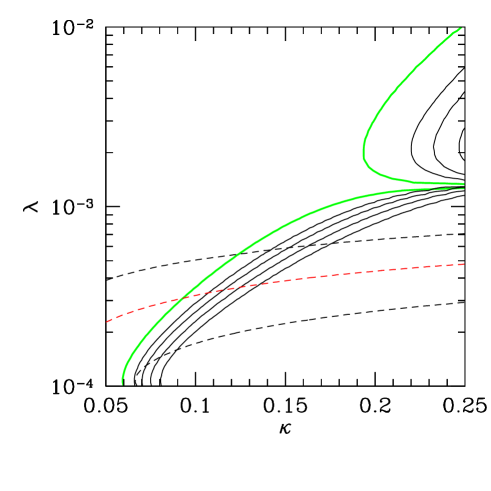
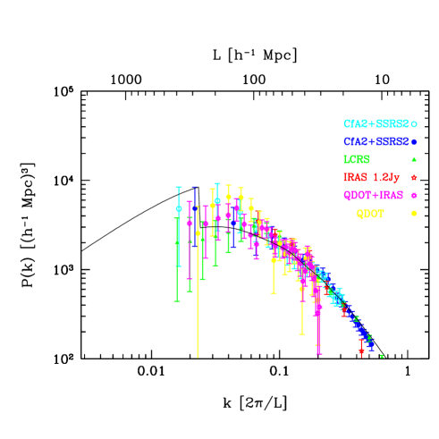
where is a CDM transfer function. We draw a sample of results in Fig.1 for . From this figure we can see that if
| (41) |
is at a cosmological scale, and density fluctuations produced during new inflation are not too far from that of preinflation. We can understand the qualitative dependence of on as follows: When is large, the slope of the potential for new inflation is too steep, and new inflation cannot last for a long time. Therefore, the break occurs at smaller scales. As for , we can see that the larger is, the larger is, from Eq.(7). In addition, from Eqs.(23) and (31), we can see that
| (42) |
for a fixed . Thus, we have larger for larger .
III Comparison with observations
In this section we compare the result of our double inflation model with the observations of the cluster abundances [17, 18] and galaxy distributions [19, 20, 21, 22, 23].
A Cluster Abundances
Since the power spectrum of density fluctuations shows a break on the cosmological scale in this double inflation model, we cannot simply employ the value of quoted by previous works [17, 18]. We need to calculate the cluster abundances by using the Press-Schechter theory [30]. According to the Press-Schechter theory, the comoving number density of collapsed systems of mass at redshift , per interval , is expressed as
| (43) |
where is the mean mass density of the universe at present, and is the mass variance, the rms density fluctuations smoothed over the mass scale , which is defined as
| (44) |
where , is a window function
| (45) |
and is a present matter density fluctuation power spectrum with a normalization . For the case of , . This is the density contrast that a collapsed region should have at collapse time if it had always evolved according to linear theory. In this paper we take total matter density and use the observations of neighbor clusters ().
Given the power spectrum, we can obtain the cluster abundance from the Press-Schechter theory. When we determine the breaking scale , the power spectrum ratio , and the spectral index for new inflation , we can get the power spectrum up to normalization . Using this power spectrum we can calculate the mass variance and obtain, from Eq.(43),
| (46) |
Many clusters of galaxies are observed using x-ray fluxes. Under the assumption that clusters are hydrostatic, we can obtain the mass-temperature relations as
| (47) |
where is the ratio of the mean density of a cluster to the critical density at that redshift, is the ratio of specific galaxy kinetic energy to specific gas thermal energy, and is the hydrogen mass fraction. We take , , and [17]. Then Eq. (47) reduces to
| (48) |
The observed cluster abundance as a function of x-ray temperature can be translated into a function of mass using Eq. (47). Accumulating the observations, Henry and Arnaud [31] gave the fitting formula as
| (49) |
By integrating Eq. (49) we obtain
| (50) |
where the unit of cluster abundance is . Henry and Arnaud [31] also gave a table of cluster observations whose temperatures are larger than keV, which corresponds to a lower limit [see Eq.(48)]. Therefore we have, from Eq. (50),
| (51) |
Matching these abundances, Eq. (46) calculated from the Press-Schechter theory, and Eq. (51) inferred from the x-ray cluster observations, we can determine the normalization (amplitude) of power spectrum, . Using this normalization, we can obtain “cluster abundance normalized” , , as
| (52) |
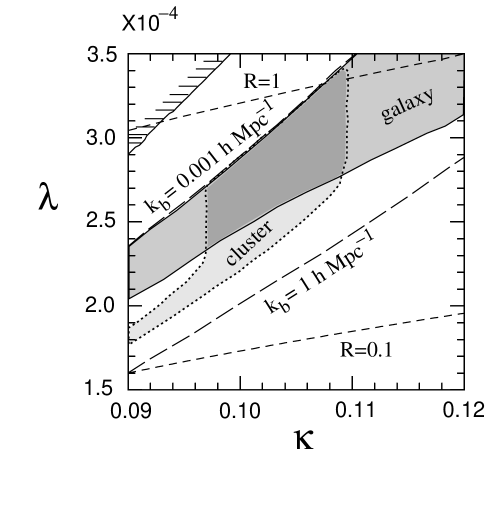
Because of error bars, we have a range of from observations. On the other hand, we can normalize the power spectrum by COBE data [11, 32]. Therefore, we have “COBE normalized” , together with . Bunn and White [32] estimates one standard deviation error of COBE normalization to be which is much smaller than the one of cluster normalization. We conclude that if lies in a range, that the parameter region of , , and is consistent with the cluster abundance observations (see lightly shaded region of Fig. 3 for ).
B galaxy distributions
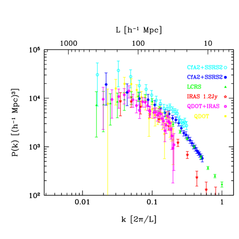
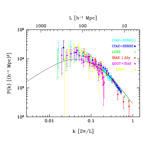
There are many observations which measure the density fluctuations from galaxy distributions. Among these we use following data sets in this paper.
-
Southern Sky Redshift Survey of optically selected galaxies (SSRS2) & The Center for Astrophysics redshift survey of the northern hemisphere (CfA2) ( volume-limited, ), analyzed by da Costa et al [19].
-
The same with above ( volume-limited, ) [19].
-
The Las Campanas Redshift Survey (LCRS), analyzed by Lin et al [20].
-
The Infrared Astronomical Satellite (IRAS) 1.2 Jy Sample, analyzed by Fisher et al [21].
-
The Queen Mary College, Durham, Oxford, and Toronto (QDOT) survey, analyzed by Feldman et al [22].
-
IRAS 1.2 Jy + QDOT [ weighting], analyzed by Tadros and Efstathiou [23].
Employing the COBE normalization, we can determine the power spectrum with its overall amplitude if we fix the the breaking scale , the power spectrum ratio , and the spectral index for new inflation . One might want to make direct comparison of this power spectrum with above observations of galaxy distributions. However, distribution of luminous objects such as galaxies could differ from underlying mass distribution because of so-called bias. There is even no guarantee that each observational sample has same bias factor. Therefore, we only consider the shape of the power spectrum here. We change the overall amplitude of each set of observations arbitrarily. And we estimate the goodness of fitting by calculating of this power spectrum with fixing , and .
In Fig. 3, we plot a sample of our results for . There is a parameter region where both the cluster abundances and galaxy distributions can be accounted for by our model. What we can see from this figure is that we have almost fixed value of and , if we require that a break should occur at a cosmological scale. The results for to are summarized in Table I (outside of this range, we cannot find a suitable parameter region), where we write the coupling constants and .
C CMB anisotropies
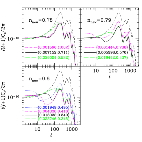
In our double inflation model, the density fluctuations at smaller scales are produced during new inflation, and they have different amplitudes from COBE normalization. Also, they are tilted in general (). Thus, the cosmic microwave background (CMB) anisotropy angular power spectrum would have a nontrivial shape at smaller scales. We choose nine parameter sets from Fig.3 [see TableII], and calculate the CMB angular power spectra (Fig.6). In the allowed parameter region, and . In this region, the characteristic feature known as the acoustic peaks is suppressed compared with the standard CDM case (dashed lines). Some of them show a dip on the scales, which correspond to the breaking scales , larger than the first peak (smaller in ). Although such recent medium angle experiments as Saskatoon [33], QMAP [34], and TOCO97/TOCO98 [35] have reported the existence of the first acoustic peak, these results are inconclusive in view of rather large observational errors. The observations of CMB anisotropies by future satellite experiments [Microwave Anisotropy Probe (MAP)[36], Planck[37]] would be able to test our models.
IV Conclusions and Discussions
In this paper we have studied the density fluctuations produced in the double inflation model in supergravity, and compared it to the observations. Our double inflation model consists of preinflation (= hybrid inflation ) and new inflation. Preinflation provides the density fluctuations observed by COBE and it also dynamically sets the initial condition of new inflation through supergravity effects. The predicted power spectrum has almost a scale-invariant form () on large cosmological scales which is favored for the structure formation of the universe [38]. On the other hand, new inflation gives the power spectrum which has different amplitude and shallow slope () on small scales. Thus, this power spectrum has a break on the scale corresponding to the turning epoch from preinflation to new inflation.
We have shown that there is a parameter region where the double inflation model produces an appropriate power spectrum, i.e., the break occurs at a cosmological scale and both cluster abundances and galaxy distributions can be accounted for.
We have also calculated the CMB angular power spectra for some appropriate parameters. In our double inflation model, the acoustic peaks are suppressed compared with the no-break model. Future satellite experiments would be able to test our model and will make precise determination of model parameters possible.
Acknowledgment
The authors thank M. Vogeley for kindly providing the data for galaxy distributions. T. K. is grateful to K. Sato for his continuous encouragement, and to T. Kitayama for useful discussions. N.S. thanks the Max Planck Institute for Astrophysics in Garching for their warm hospitality. A part of work is supported by Grant-in-Aid from the Ministry of Education.
REFERENCES
- [1] A. H. Guth, Phys. Rev. D23, 347 (1981).
- [2] K. Sato, Mon. Not. R. Astron. Soc. 195, 467 (1981); A. A. Starobinsky, Pis’ma Zh. Éksp. Teor. Fiz. 30, 719 81979) [JETP Lett. 30, 682 (1979)]; Phys. Lett. B91, 99 (1980).
- [3] For example, A.D. Linde, Particle Physics and Inflationary Cosmology (Harwood, Chur, Switzerland, 1990).
- [4] A. D. Linde, Phys. Lett. B129, 177 (1983).
- [5] A. Albrecht and P.J. Steinhardt, Phys. Rev. Lett. 48, 1220 (1982); A.D. Linde, Phys. Lett. B108, 389 (1982).
- [6] A. D. Linde, Phys. Rev. D49, 748 (1994); E. J. Copeland, A. R. Liddle, D. H. Lyth, E. D. Stewart, and D. Wands, ibid. D49, 6410 (1994).
- [7] M. Yu. Khlopov and A.D. Linde, Phys. Lett. B138, 265 (1984) ; J. Ellis, E. Kim and D.V. Nanopoulos, ibid.B145, 181 (1984); J. Ellis, G.B. Gelmini, J.L. Lopez, D.V. Nanopoulos, and S. Sarker, Nucl. Phys. B373, 399 (1992); M. Kawasaki and T. Moroi, Prog. Theor. Phys. 93, 879 (1995).
- [8] T. Moroi, H. Murayama, and M. Yamaguchi, Phys. Lett. B303, 289 (1993).
- [9] K.I. Izawa, M. Kawasaki, and T. Yanagida, Phys. Lett. B411, 249 (1997).
- [10] E. W. Kolb and M. S. Turner, The Early Universe (Addison-Wesley, Reading MA, 1990).
- [11] C.L. Bennett et al., Astrophys. J. 464, L1 (1996).
- [12] M. Kawasaki, N. Sugiyama, and T. Yanagida, Phys. Rev. D57, 6050 (1998).
- [13] M. Kawasaki and T. Yanagida, Phys. Rev. D59, 043512 (1999).
-
[14]
L.A. Kofman, A.D. Linde, and A.A. Starobinsky,
Phys. Lett. B 157, 361 (1985); J. Silk and M.S. Turner, Phys.
Rev. D 35, 419 (1987); D. Polarski and A.A. Starobinsky, Nucl.
Phys. B 385, 623 (1992);
P. Peter, D. Polarski, and A.A. Starobinsky, Phys. Rev. D 50, 4827 (1994); S. Gottlöber, J. P. Mücket, and A. A. Starobinsky, Astrophys. J. 434, 417 (1994); R. Kates, V. Müller, S. Gottlöber, J. P. Mücket, and J. Retzlaff, Mon. Not. Roy. Astron. Soc. 277, 1254 (1995); J.A. Adams, G.G. Ross, and S. Sarkar, Nucl. Phys. B 503, 405 (1997); J. Lesgourgues and D. Polarski, Phys. Rev. D 56, 6425 (1997); J. Lesgourgues, D. Polarski and A.A. Starobinsky, Mon. Not. Roy. Astron. Soc. 297, 769 (1998); M. Sakellariadou and N. Tetradis, hep-ph/9806461. - [15] I. Dominguez, P. Hoeflich, O. Straniero, and C. Wheeler, astro-ph/9905047; P. S. Drell, T. J. Loredo, and I. Wasserman, astro-ph/9905027; A. N. Aguirre, astro-ph/9904319; A. G. Riess, A. V. Filippenko, W. Li and B. P. Schmidt, astro-ph/9907038.
- [16] C. Panagiotakopoulous, Phys. Rev. D55, 7335 (1997); A. Linde and A. Riotto, ibid.56, R1841 (1997).
- [17] V. Eke, S. Cole, and C. S. Frenk, Mon. Not. R. Astron. Soc. 282, 263 (1996).
- [18] P. T. P. Viana and A. R. Liddle, in Proceedings of the Conference “Cosmological Constraints from X-Ray Clusters”, astro-ph/9902245.
- [19] L. N. da Costa et al., Astrophys. J. 437, L1 (1994).
- [20] H. Lin et al., Astrophys. J. 471, 617 (1996).
- [21] K. B. Fisher et al., Astrophys. J. 402, 42 (1993).
- [22] H. A. Feldman, N. Kaiser, and J. A. Peacock, Astrophys. J. 426, 23 (1994).
- [23] H. Tadros and G. Efstathiou, Mon. Not. R. Astron. Soc. 276, L45 (1995).
- [24] M. S. Vogeley, in The Evolving Universe, edited by D. Hamilton (Kluwer, Dordrecht, 1998), p.395.
- [25] K.I. Izawa and T. Yanagida, Phys. Lett. B393, 331 (1997).
- [26] G. Dvali, Q. Shafi, and R.K. Shaefer, Phys. Rev. Lett. 73, 1886 (1994).
- [27] K. Kumekawa, T. Moroi, and T. Yanagida, Prog. Theor. Phys. 92, 437 (1994); M. Dine, L. Randall, and S. Thomas, Phys. Rev. Lett. 75, 398 (1995).
- [28] K. Enquvist, K.W. Ng, and K.A. Olive, Nucl. Phys. B303, 713 (1988).
- [29] A. R. Liddle and D. H. Lyth, Phys. Rep. 231, 1 (1995).
- [30] W. H. Press and P. Schechter, Astrophys. J. 187, 425 (1974).
- [31] J. P. Henry and K. A. Arnaud, Astrophys. J. 372, 410 (1991).
- [32] E. F. Bunn and M. White, Astrophys. J. 480, 6 (1997)
- [33] C. B. Netterfield et al., Astrophys. J. 474, 47 (1997).
- [34] A. de Oliveira-Costa et al., Astrophys. J. 509, L77 (1998).
- [35] E. Torbet et al., Astrophys. J. 521, L79 (1999); A. D. Miller et al., astro-ph/9906421.
- [36] http://map.gsfc.nasa.gov
- [37] http://astro.estec.esa.nl/SA-general/Projects/Planck/
- [38] M. White, D. Scott, J. Silk, and M. Davis, Mon. Not. R. Astron. Soc. 276, L69 (1995).
| Mpc) | ||||
|---|---|---|---|---|