$CP$- and $T$-Violation in the Decay
$K_{L}\rightarrow\pi^{+}\pi^{-}e^{+}e^{-}$ and Related Processes

Abstract

I review the theoretical basis of the prediction that the decay $K_{L}\rightarrow\pi^{+}\pi^{-}e^{+}e^{-}$ should show a large $CP$- and $T$-violation, a prediction now confirmed by the KTeV experiment. The genesis of the effect lies in a large violation of $CP$- and $T$-invariance in the decay $K_{L}\rightarrow\pi^{+}\pi^{-}\gamma$, which is encrypted in the polarization state of the photon. The decay $K_{L}\rightarrow\pi^{+}\pi^{-}e^{+}e^{-}$ serves as an analyser of the photon polarization. The asymmetry in the distribution of the angle $\phi$ between the $\pi^{+}\pi^{-}$ and $e^{+}e^{-}$ planes is a direct measure of the $CP$-odd, $T$-odd component of the photon’s Stokes vector. A complete study of the angular distribution can reveal further $CP$-violating features, which probe the non-radiative (charge-radius and short-distance) components of the $K_{L}\rightarrow\pi^{+}\pi^{-}e^{+}e^{-}$ amplitude.

Eight years ago, there appeared a report [1] by the E-731 experiment concerning the branching ratio and photon energy spectrum of the decays $K_{L,S}\rightarrow\pi^{+}\pi^{-}\gamma$. It was found that while the $K_{S}$ decay could be well-reproduced by inner bremsstrahlung from an underlying process $K_{S}\rightarrow\pi^{+}\pi^{-}$, the $K_{L}$ decay contained a mixture of a bremsstrahlung component ($I\!B$) and a direct emission component ($D\!E$), the relative strength being $D\!E/(D\!E+I\!B)=0.68$ for photons above $20\,MeV$. The simplest matrix element consistent with these features is

$$\mathcal{M}(K_{S}\rightarrow\pi^{+}\pi^{-}\gamma) = ef_{S}\left[\frac{\epsilon\cdot p_{+}}{k\cdot p_{+}}-\frac{\epsilon\cdot p_{-}}{k\cdot p_{-}}\right]$$ (1)

$$\mathcal{M}(K_{L}\rightarrow\pi^{+}\pi^{-}\gamma) = ef_{L}\left[\frac{\epsilon\cdot p_{+}}{k\cdot p_{+}}-\frac{\epsilon\cdot p_{-}}{k\cdot p_{-}}\right]+e\frac{f_{DE}}{{M_{K}}^{4}}\epsilon_{\mu\nu\rho\sigma}\epsilon^{\mu}k^{\nu}{p_{+}}^{\rho}{p_{-}}^{\sigma}$$

where

$$f_{L}\equiv|f_{S}|g_{Br},\>g_{Br}=\eta_{+-}e^{i\delta_{0}(s={M_{K}}^{2})},$$

$$f_{DE}\equiv|f_{S}|g_{M1},\>g_{M1}=i(0.76)e^{i\delta_{1}(s)}.$$ (2)

Here the direct emission has been represented by a $CP$-conserving magnetic dipole coupling $g_{M1}$, whose magnitude $|g_{M1}|=0.76$ is fixed by the empirical ratio $DE/IB$. The phase factors appearing in $g_{Br}$ and $g_{M1}$ are dictated by the Low theorem for bremsstrahlung, and the Watson theorem for final state interactions. The factor $i$ in $g_{M1}$ is a consequence of $CPT$ invariance [2]. The matrix element for $K_{L}\rightarrow\pi^{+}\pi^{-}\gamma$ contains simultaneously electric multipoles associated with bremsstrahlung ($E1,\,E3,\,E5$ …), which have $CP=+1$, and a magnetic $M1$ multipole with $CP=-1$. It follows that interference of the electric and magnetic emissions should give rise to $CP$-violation.

To understand the nature of this interference, we write the $K_{L}\rightarrow\pi^{+}\pi^{-}\gamma$ amplitude more generally as

$$\mathcal{M}(K_{L}\rightarrow\pi^{+}\pi^{-}\gamma) = \frac{1}{{M_{K}}^{3}}\left\{E(\omega,\cos\theta)\left[\epsilon\cdot p_{+}\,k\cdot p_{-}-\epsilon\cdot p_{-}\,k\cdot p_{+}\right]\right.$$ (3)

$$\left.\mbox{}+M(\omega,\cos\theta)\epsilon_{\mu\nu\rho\sigma}\epsilon^{\mu}k^{\nu}{p_{+}}^{\rho}{p_{-}}^{\sigma}\right\}$$

where $\omega$ is the photon energy in the $K_{L}$ rest frame, and $\theta$ is the angle between $\pi^{+}$ and $\gamma$ in the $\pi^{+}\pi^{-}$ rest frame. In the model represented by Eqs. (1) and (2), the electric and magnetic amplitudes are

$$E = \left(\frac{2M_{K}}{\omega}\right)^{2}\frac{g_{Br}}{1-\beta^{2}\cos^{2}\theta}$$

$$M = g_{M1}$$ (4)

where $\beta=(1-4{m_{\pi}}^{2}/s)^{1/2}$, $\sqrt{s}$ being the $\pi^{+}\pi^{-}$ invariant mass. The Dalitz plot density, summed over photon polarizations is

$$\frac{d\Gamma}{d\omega\,d\!\cos\theta}=\frac{1}{512\pi^{3}}\left(\frac{\omega}{M_{K}}\right)^{3}\beta^{3}\left(1-\frac{2\omega}{M_{K}}\right)\sin^{2}\theta\left[|E|^{2}+|M|^{2}\right]$$ (5)

Clearly, there is no interference between the electric and magnetic multipoles if the photon polarization is unobserved. Therefore, any $CP$-violation involving the interference of $g_{Br}$ and $g_{M1}$ is hidden in the polarization state of the photon.

The photon polarization can be defined in terms of the density matrix

$$\rho=\left(\begin{array}[]{cc}|E|^{2}&E^{*}M\\ EM^{*}&|M|^{2}\end{array}\right)=\frac{1}{2}\left(|E|^{2}+|M|^{2}\right)\left[1\!\!\!\!\>\>\mbox{l}+\vec{S}\cdot\vec{\tau}\right]$$ (6)

where $\vec{\tau}=(\tau_{1},\,\tau_{2},\,\tau_{3})$ denotes the Pauli matrices, and $\vec{S}$ is the Stokes vector of the photon with components

$$S_{1} = 2Re\left(E^{*}M\right)/\left(|E|^{2}+|M|^{2}\right)$$

$$S_{2} = 2Im\left(E^{*}M\right)/\left(|E|^{2}+|M|^{2}\right)$$ (7)

$$S_{3} = \left(|E|^{2}-|M|^{2}\right)/\left(|E|^{2}+|M|^{2}\right).$$

The component $S_{3}$ measures the relative strength of the electric and magnetic radiation at a given point in the Dalitz plot. The effects of $CP$-violation reside in the components $S_{1}$ and $S_{2}$, which are proportional to $Re\,({g_{Br}}^{*}g_{M1})$ and $Im\,({g_{Br}}^{*}g_{M1})$, respectively. Of these $S_{1}$ is $CP$-odd, $T$-odd, while $S_{2}$ is $CP$-odd, $T$-even. Physically, $S_{2}$ is the net circular polarization of the photon: such a polarization is known to be possible in decays like $K_{L}\rightarrow\pi^{+}\pi^{-}\gamma$ or $K_{L,S}\rightarrow\gamma\gamma$ whenever there is $CP$-violation accompanied by unitarity phases [3]. To understand the significance of $S_{1}$, we examine the dependence of the $K_{L}\rightarrow\pi^{+}\pi^{-}\gamma$ decay on the angle $\phi$ between the polarization vector $\vec{\epsilon}$ and the unit vector $\vec{n}_{\pi}$ normal to the $\pi^{+}\pi^{-}$ plane (we choose coordinates such that $\vec{k}=(0,\,0,\,k)$, $\vec{n}_{\pi}=(1,\,0,\,0)$, $\vec{p}_{+}=(0,\,p\sin\theta,\,p\cos\theta)$ and $\vec{\epsilon}=(\cos\phi,\,\sin\phi,\,0)$):

$$\frac{d\Gamma}{d\omega\,d\!\cos\theta\,d\phi}\sim\left|E\sin\phi-M\cos\phi\right|^{2}\sim 1-\left[S_{3}\cos 2\phi+S_{1}\sin 2\phi\right]$$ (8)

Thus the $CP$-odd, $T$-odd Stokes parameter $S_{1}$ appears as a coefficient of the term $\sin 2\phi$. The essential idea of Refs. [4, 5] is to use in place of $\vec{\epsilon}$, the vector $\vec{n}_{l}$ normal to the plane of the Dalitz pair in the reaction $K_{L}\rightarrow\pi^{+}\pi^{-}\gamma^{*}\rightarrow\pi^{+}\pi^{-}e^{+}e^{-}$. This motivates the study of the distribution $d\Gamma/d\phi$ in the decay $K_{L}\rightarrow\pi^{+}\pi^{-}e^{+}e^{-}$, where $\phi$ is the angle between the $\pi^{+}\pi^{-}$ and $e^{+}e^{-}$ planes.

To obtain a quantitative idea of the magnitude of $CP$- violation in $K_{L}\rightarrow\pi^{+}\pi^{-}\gamma$, we show in Fig. 1a the three components of the Stokes vector as a function of the photon energy [6]. These are calculated from the amplitudes (4) using weighted averages of $|E|^{2}$, $|M|^{2}$, $E^{*}M$ and $EM^{*}$ over $\cos\theta$. The values of $S_{1}$ and $S_{2}$ are remarkably large, considering that the only source of $CP$-violation is the $\epsilon$-impurity in the $K_{L}$ wave-function ($\epsilon=\eta_{+-}$). Clearly the $1/\omega^{2}$ factor in $E$ enhances it to a level that makes it comparable to the $CP$-conserving amplitude $M$. This is evident from the behaviour of the parameter $S_{3}$, which swings from a dominant electric behaviour at low $E_{\gamma}$ ($S_{3}\approx 1$) to a dominant magnetic behaviour at large $E_{\gamma}$ ($S_{3}\approx-1$), with a zero in the region $E_{\gamma}\approx 60\,MeV$. To highlight the difference between the $T$-odd parameter $S_{1}$ and the $T$-even parameter $S_{2}$, we show in Fig. 1b the behaviour of the Stokes parameters in the “hermitian limit”: this is the limit in which the $T$-matrix or effective Hamiltonian governing the decay $K_{L}\rightarrow\pi^{+}\pi^{-}\gamma$ is taken to be hermitian, all unitarity phases related to real intermediate states being dropped. This limit is realized by taking $\delta_{0},\,\delta_{1}\rightarrow 0$, and $ar\!g\,\epsilon\rightarrow\pi/2$. The last of these follows from the fact that $\epsilon$ may be written as

$$\epsilon=\frac{\Gamma_{12}-\Gamma_{21}+i\left(M_{12}-M_{21}\right)}{\gamma_{S}-\gamma_{L}-2i\left(m_{L}-m_{S}\right)}$$ (9)

where $H_{eff}=M-i\Gamma$ is the mass matrix of the $K^{0}$-$\overline{K}^{0}$ system. The hermitian limit obtains when $\Gamma_{12}=\Gamma_{21}=\gamma_{S}=\gamma_{L}=0$. As seen from Fig. 1b, $S_{2}$ vanishes in this limit, but $S_{1}$ survives, as befits a $CP$-odd, $T$-odd parameter. Fig. 1c shows what happens in the $CP$-invariant limit $\epsilon\rightarrow 0$. It is clear that we are dealing here with a dramatic situation in which a $CP$-impurity of a few parts in a thousand in the $K_{L}$ wave-function gives rise to a huge $CP$-odd, $T$-odd effect in the photon polarization.

We can now examine how these large $CP$-violating effects are transported to the decay $K_{L}\rightarrow\pi^{+}\pi^{-}e^{+}e^{-}$. The matrix element for $K_{L}\rightarrow\pi^{+}\pi^{-}e^{+}e^{-}$ can be written as [4, 5]

$$\mathcal{M}(K_{L}\rightarrow\pi^{+}\pi^{-}e^{+}e^{-})=\mathcal{M}_{br}+\mathcal{M}_{mag}+\mathcal{M}_{CR}+\mathcal{M}_{SD}.$$ (10)

Here $\mathcal{M}_{br}$ and $\mathcal{M}_{mag}$ are the conversion amplitudes associated with the bremsstrahlung and $M1$ parts of the $K_{L}\rightarrow\pi^{+}\pi^{-}\gamma$ amplitude. In addition, we have introduced an amplitude $\mathcal{M}_{CR}$ denoting $\pi^{+}\pi^{-}$ production in a $J=0$ state (not possible in a real radiative decay), as well as an amplitude $\mathcal{M}_{SD}$ associated with the short-distance interaction $s\rightarrow d\,e^{+}e^{-}$. The last of these turns out to be numerically negligible because of the smallness of the $C\!K\!M$ factor $V_{ts}{V_{td}}^{*}$. The $s$-wave amplitude $\mathcal{M}_{CR}$, if approximated by the $K^{0}$ charge radius diagram, makes a small ($\sim 1\%$) contribution to the decay rate. Thus the dominant features of the decay are due to the conversion amplitude $\mathcal{M}_{br}+\mathcal{M}_{mag}$.

Within such a model, one can calculate the differential decay rate in the form [5]

$$d\Gamma=I(s_{\pi},\,s_{l},\,\cos\theta_{l},\,\cos\theta_{\pi},\,\phi)\,ds_{\pi}\,ds_{l}\,d\!\cos\theta_{l}\,d\!\cos\theta_{\pi}\,d\phi.$$ (11)

Here $s_{\pi}$ ($s_{l}$) is the invariant mass of the pion (lepton) pair, and $\theta_{\pi}$ ($\theta_{l}$) is the angle of the $\pi^{+}$ ($l^{+}$) in the $\pi^{+}\pi^{-}$ ($l^{+}l^{-}$) rest frame, relative to the dilepton (dipion) momentum vector in that frame. The all-important variable $\phi$ is defined in terms of unit vectors constructed from the pion momenta $\vec{p_{\pm}}$ and lepton momenta $\vec{k_{\pm}}$ in the $K_{L}$ rest frame:

$$\vec{n}_{\pi}=\left(\vec{p}_{+}\times\vec{p}_{-}\right)/\left|\vec{p}_{+}\times\vec{p}_{-}\right|, \vec{n}_{l}=\left(\vec{k}_{+}\times\vec{k}_{-}\right)/\left|\vec{k}_{+}\times\vec{k}_{-}\right|,$$

$$\vec{z}=\left(\vec{p}_{+}+\vec{p}_{-}\right)/\left|\vec{p}_{+}+\vec{p}_{-}\right|,$$

$$\sin\phi\>= \vec{n}_{\pi}\times\vec{n}_{l}\cdot\vec{z} (CP=-,T=-),$$ (12)

$$\cos\phi\>= \vec{n}_{l}\cdot\vec{n}_{\pi} (CP=+,T=+).$$

In Ref. [4], an analytic expression was derived for the 3-dimensional distribution $d\Gamma/ds_{l}\,ds_{\pi}\,d\phi$, which has been used in the Monte Carlo simulation of this decay. In Ref. [5], a formalism was presented for obtaining the fully differential decay function $I(s_{\pi},\,s_{l},\,\cos\theta_{l},\,\cos\theta_{\pi},\phi)$.

The principal results of the theoretical model discussed in [4, 5] are as follows:

1. Branching ratio: This was calculated to be [4]

$$B\!R(K_{L}\rightarrow\pi^{+}\pi^{-}e^{+}e^{-}) = (1.3\times 10^{-7})_{Br}+(1.8\times 10^{-7})_{M1}$$ (13)

$$\mbox{}+(0.04\times 10^{-7})_{CR}\approx 3.1\times 10^{-7},$$

which agrees well with the result $(3.32\pm 0.14\pm 0.28)\times 10^{-7}$ measured in the KTeV experiment [7]. (A preliminary branching ratio $2.9\times 10^{-7}$ has been reported by NA48 [8]).

2. Asymmetry in $\phi$ distribution: The model predicts a distribution of the form

$$\frac{d\Gamma}{d\phi}\sim 1-\left(\Sigma_{3}\cos 2\phi+\Sigma_{1}\sin 2\phi\right)$$ (14)

where the last term is $CP$- and $T$-violating, and produces an asymmetry

$$\mathcal{A}=\frac{\left(\int_{0}^{\pi/2}-\int_{\pi/2}^{\pi}+\int_{\pi}^{3\pi/2}-\int_{3\pi/2}^{2\pi}\right)\frac{d\Gamma}{d\phi}d\phi}{\left(\int_{0}^{\pi/2}+\int_{\pi/2}^{\pi}+\int_{\pi}^{3\pi/2}+\int_{3\pi/2}^{2\pi}\right)\frac{d\Gamma}{d\phi}d\phi}=-\frac{2}{\pi}\Sigma_{1}.$$ (15)

The predicted value [4, 5] is

$$|\mathcal{A}|=15\%\,\sin(\phi_{+-}+\delta_{0}({M_{K}}^{2})-\overline{\delta}_{1})\approx 14\%$$ (16)

to be compared with the KTeV result [7]

$$|\mathcal{A}|_{KTeV}=(13.6\pm 2.5\pm 1.2)\%$$ (17)

The “Stokes parameters” $\Sigma_{3}$ and $\Sigma_{1}$ are calculated to be $\Sigma_{3}=-0.133$, $\Sigma_{1}=0.23$. The $\phi$-distribution measured by KTeV agrees with this expectation (after acceptance corrections made in accordance with the model). It should be noted that the sign of $\Sigma_{1}$ (and of the asymmetry $\mathcal{A}$) depends on whether the numerical coefficient in $g_{M1}$ is taken to be $+0.76$ or $-0.76$. The data happen to support the positive sign chosen in Eq. (2).

3. Variation of Stokes parameters with $s_{\pi}$: As shown in Fig. 1d, the parameters $\Sigma_{1}$ and $\Sigma_{3}$ have a variation with $s_{\pi}$ that is in close correspondence with the variation of $S_{1}$ and $S_{3}$ shown in Fig. 1. (Recall that the photon energy $E_{\gamma}$ in $K_{L}\rightarrow\pi^{+}\pi^{-}\gamma$ can be expressed in terms of $s_{\pi}$: $s_{\pi}={M_{K}}^{2}-2M_{K}E_{\gamma}$.) In particular the zero of $\Sigma_{3}$ and the zero of $S_{3}$ occur at almost the same value of $s_{\pi}$. This variation with $s_{\pi}$ combined with the low detector acceptance at large $s_{\pi}$, has the consequence of enhancing the measured asymmetry ($23.3\pm 2.3\%$ in KTeV [7], $20\pm 5\%$ in NA48 [8]).

4. Generalized Angular Distribution: As shown in Ref. [5], a more complete study of the angular distribution of the decay $K_{L}\rightarrow\pi^{+}\pi^{-}e^{+}e^{-}$ can yield further $CP$-violating observables, some of which are sensitive to the non-radiative (charge-radius and short-distance) parts of the matrix element. In particular the two-dimensional distribution $d\Gamma/d\!\cos\theta_{l}d\phi$ has the form

$$\frac{d\Gamma}{d\!\cos\theta_{l}d\phi} = K_{1}+K_{2}\cos 2\theta_{l}+K_{3}\sin^{2}\theta_{l}\cos 2\phi+K_{4}\sin 2\theta_{l}\cos\phi$$ (18)

$$\mbox{}+K_{5}\sin\theta_{l}\cos\phi+K_{6}\cos\theta_{l}+K_{7}\sin\theta_{l}\sin\phi$$

$$\mbox{}+K_{8}\sin 2\theta_{l}\sin\phi+K_{9}\sin^{2}\theta_{l}\sin 2\phi.$$

Considering the behaviour of $\cos\theta_{l}$, $\sin\theta_{l}$, $\cos\phi$ and $\sin\phi$ under $CP$ and $T$, the various terms appearing in Eq. (18) have the following transformation:

	$CP$	$T$
$K_{1}$, $K_{2}$, $K_{3}$, $K_{5}$	+	+
$K_{4}$, $K_{6}$	$-$	+
$K_{8}$	+	$-$
$K_{7}$, $K_{9}$	$-$	$-$

Note that $K_{4,6,8}$ have $(CP)(T)=-$, a signal that they vanish in the hermitian limit. If only the bremsstrahlung and magnetic dipole terms are retained in the $K_{L}\rightarrow\pi^{+}\pi^{-}e^{+}e^{-}$ amplitude, one finds $K_{4}=K_{5}=K_{6}=K_{7}=K_{8}=0$, the only non-zero coefficients being $K_{1}=1$ (norm), $K_{2}=0.297$, $K_{3}=0.180$, $K_{9}=-0.309$. In this notation, the asymmetry in $d\Gamma/d\phi$ is $\mathcal{A}=\frac{2}{\pi}\frac{\frac{2}{3}K_{9}}{1-\frac{1}{3}K_{2}}=-14\%$. The introduction of a charge-radius term induces a new $CP$-odd, $T$-even term $K_{4}\approx-1.3\%$, while a short-distance interaction containing an axial vector electron current can induce the $CP$-odd, $T$-odd term $K_{7}$. The standard model prediction for $K_{7}$, however, is extremely small.

We conclude with a list of questions that could be addressed by future research. In connection with $K_{L,S}\rightarrow\pi^{+}\pi^{-}\gamma$: (i) Is there a departure from bremsstrahlung in $K_{S}\rightarrow\pi^{+}\pi^{-}\gamma$ (evidence for direct $E1$)? (ii) Is there a $\pi^{+}/\pi^{-}$ asymmetry in $K_{L}\rightarrow\pi^{+}\pi^{-}\gamma$ (evidence for $E2$)? (iii) Is there a measurable difference between $\eta_{+-\gamma}$ and $\eta_{+-}$ (existence of direct $CP$-violating $E1$ in $K_{L}\rightarrow\pi^{+}\pi^{-}\gamma$)? With respect to the decay $K_{L}\rightarrow\pi^{+}\pi^{-}e^{+}e^{-}$: (i) Is there evidence of an $s$-wave amplitude? (ii) Is there evidence for $K_{4}$ or $K_{7}$ types of $CP$-violation? On the theoretical front: (i) Can one calculate the $s$-wave amplitude, and the form factors in $K_{L}\rightarrow\pi^{+}\pi^{-}\gamma^{*}$ [9]? (ii) Can one understand the sign of $g_{M1}$? (iii) Can one explain why direct $E1$ in $K_{S}\rightarrow\pi^{+}\pi^{-}\gamma$ is so small compared to direct $M1$ in $K_{L}\rightarrow\pi^{+}\pi^{-}\gamma$ ($\left|g_{E1}/g_{M1}\right|<5\%$)?

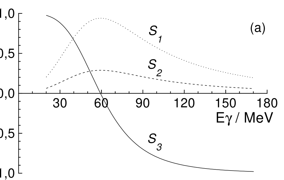
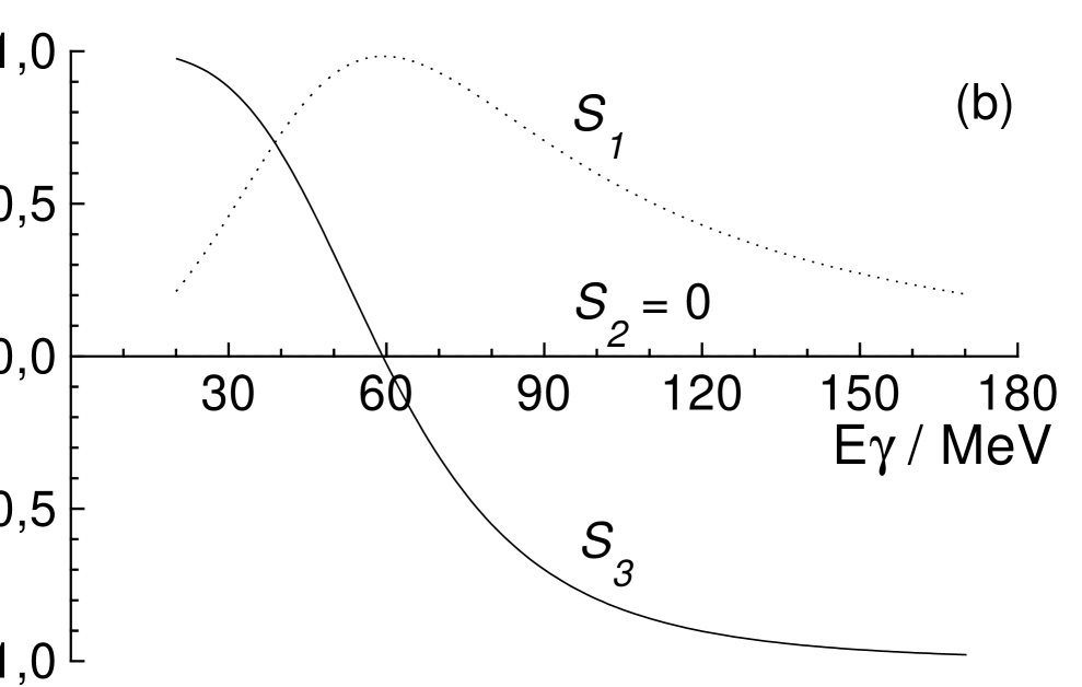
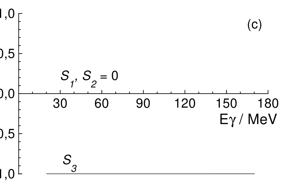
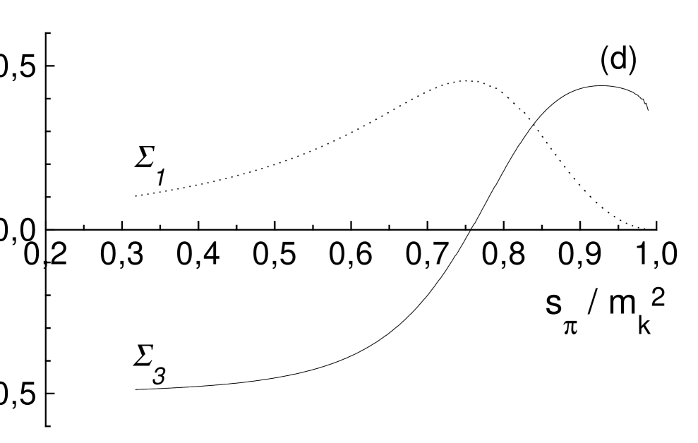
Figure 1: (a) Stokes parameters of photon in $K_{L}\rightarrow\pi^{+}\pi^{-}\gamma$; (b) Hermitian limit $\delta_{0}=\delta_{1}=0$, $ar\!g\,\epsilon=\pi/2$; (c) $CP$-invariant limit $\epsilon\rightarrow 0$; (d) “Stokes parameters” for $K_{L}\rightarrow\pi^{+}\pi^{-}e^{+}e^{-}$.

References

[1] E. J. Ramberg et al., Fermilab Report No.
Fermilab-Conf-91/258,1991; Phys. Rev. Lett. 70, 2525 (1993).
[2] T. D. Lee and C. S. Wu, Annu. Rev. Nucl. Sci.
16, 511 (1966); G. Costa and P. K. Kabir, Nuovo Cimento A
61, 564 (1967); L. M. Sehgal and L. Wolfenstein, Phys. Rev.
162, 1362 (1967).
[3] L. M. Sehgal, Phys. Rev. D 4, 267 (1971).
[4] L. M. Sehgal and M. Wanninger, Phys. Rev. D
46, 1035 (1992); ibid.. D 46, 5209(E) (1992).
[5] P. Heiliger and L. M. Sehgal, Phys. Rev. D
48, 4146 (1993).
[6] L. M. Sehgal and J. van Leusen, (in preparation).
[7] KTeV collaboration, A. Alavi-Harati et al.,
hep-ex/9908020, submitted to Phys. Rev. Lett.;
A. Ledovskoy, these Proceedings.
[8] NA48 collaboration, S. Wronka, these Proceedings.
[9] M. Savage, these Proceedings.