DESY 99-108
TAUP 2592 - 99
hep-ph/9908317
Solution to the evolution equation
for high parton density QCD

Abstract

In this paper a solution is given to the nonlinear equation which describes the evolution of the parton cascade in the case of the high parton density. The related physics is discussed as well as some applications to heavy ion-ion collisions.

1 Introduction

During the past two decades one of the challenging problem of QCD has been to understand theoretically and to observe experimentally a new nonperturbative regime - high parton density QCD. It has been argued [1] in perturbative QCD (pQCD) that at low $x$ ( high energies ) the density of parton increases in deep inelastic scattering ( DIS ) and reaches so high value that partons become densely populated in a hadron. Certainly, high density system of partons cannot be treated perturbatively but pQCD leads to a new scale ( mean transverse momentum of partons ) for high parton density QCD (hdQCD ) as well as to a hypothesis of parton saturation [1]. Intensive theoretical studies led to deeper understanding of physics of this system as well as to development of both perturbative [2] and nonperturbative [3] methods for such a system. However, only recently the first indications on parton saturation have appeared in HERA data on $Q^{2}$ - behaviour of the $F_{2}$-slope and on energy behaviour of inclusive diffractive dissociation in DIS [4]. These data as well as their theoretical interpretation [5] mark a new stage of our approach which needs more quantitive methods, than it was before, to make a reliable prediction for the experimental observations.

This quantitive approach includes at least two steps:

1. a derivation of the equation which will be valid in the full kinematic region;

2. finding a solution to this equation.

There are two versions of the nonlinear evolution equation at $x\,\,\rightarrow\,\,0$. The first one was suggested as an obvious generalization of pQCD approach [6] while the second has been obtained from semiclassical gluon field approach [7]. Both of them describe correctly the DGLAP [8] evolution in the limit of low parton density as well as the GLR nonlinear evolution equation [1] in the region of intermediate parton densities. They give the same limit of parton density saturation at very low values of $x$ but they are different in particular description how system reaches this saturation. Yu. Kovchegov has recently proved [9] that the GLR equation itself (in the form of Eq.(2.18) in Ref. [1] ) is able to describe the QCD evolution in the region of high parton density or, in other words, at very low values of $x$. His arguments, which we review briefly in the next section, are based on Mueller’s idea [10] that colour dipoles rather than quarks and gluons, are correct degrees of freedom at high energies ( low $x$ ) in QCD. It was also shown that the solution to the equation, suggested in Ref.[6], coincides with the solution to the GLR equation.

The goal of this paper is to solve the GLR equation, written in the form suggested in Ref. [9], in the full kinematic region including $x\,\rightarrow\,0$. The paper is organized as follows: In the next section we briefly discuss the nonlinear evolution equation for the high parton density QCD and we formulate our approach for searching a solution to this equation. In section 3 we introduce the new scale $Q_{0}(x)$ , which appears in hdQCD as a solution to the nonlinear equation, and we find the general solution to the equation for parton with $Q^{2}\,\,>\,\,Q^{2}_{0}(x)$, based on the approach developed in Ref.[11]. Section 4 is devoted to a solution of the hdQCD equations in the region of very low $x$. We show that the parton density reaches the saturation limit and we find the explicit analytic expression describing how the system approaches the saturation limit. Our summary and conclusions are given in section 5.

2 Nonlinear equation for high density parton system

2.1 Kinematics, notations and definitions.

In this subsection we introduce all notations and definitions as well as some kinematic relations that we will need in what follows. In general, we try to use the same notation as in Ref.[9]. We would like to clarify the relations between different notations and definitions that have been used in this area of activity. This task is rather complicated since different notations have been used for the same physics observables, mostly due to different theoretical background of authors. In this paper we explore the main physical idea of Ref. [10], namely, that correct degrees of freedom in QCD at low $x$ ( high energy ) are colour dipoles rather than quarks and gluons that explicitly written in the QCD Lagrangian. This statement means that a QCD interactions at high energy do not change the size and the energy of a colour dipole. Therefore, the majority of our variables and observables is related to distributions and interactions of the colour dipoles in a hadron.

1. $\mathbf{x_{i\,k}=|\vec{x}_{i}\,-\,\vec{x}_{k}|}$ is the size of the dipole which consists of a quark $``i"$ at $\mathbf{\vec{x}_{i}}$ and an antiquark $``k"$ at $\mathbf{\vec{x}_{k}}$, or, in other words, it is the transverse separation between quark and antiquark in a colour dipole;

2. $r\,\,=\,\,\ln\frac{\mathbf{x^{2}_{0}}}{\mathbf{x^{2}}}\,\,=\,\,\ln\frac{Q^{2}}{Q^{2}_{0}}$, where $Q^{2}$ ( $Q^{2}_{0}$) is the transverse momentum of quark in the dipole with size $\mathbf{x}$ ( $\mathbf{x_{0}}$ ) respectively;

3. $x$ is the Bjorken variable for a dipole , $x=Q^{2}/W^{2}$, where $W$ is the dipole energy;

4. $y=\ln(x_{0}/x)$, where $x_{0}$ is defined for us the region of low $x$. We consider that for $x\,<\,x_{0}$ all the typical features of low $x$ physics should be seen. Practically, $x_{0}\,\approx\,10^{-2}$;

5. $xG(x,Q^{2})$ is the gluon structure function for a nucleon;

6. $xG_{A}(x,Q^{2})$ is the gluon structure function for a nucleus with A nucleons;

7. $b_{t}$ is the impact parameter for the dipole scattering;

8. The main physical observable, which we are going to discuss in this paper, is the density of dipoles ( $N({\mathbf{x}},b_{t},y)$) with the size $\mathbf{x}$ and energy $x$ ( $y$ ) at the impact parameter $b_{t}$;

9. In the parton approach ( parton $\equiv$ dipole ) the dipole density $N({\mathbf{x}},b_{t},y)$ is related to the dipole scattering amplitude if we assume that this amplitude is dominantly imaginary. Therefore, $N({\mathbf{x}},b_{t},y)$ can be normalized using the unitarity constrains:

   $$2\,\,N({\mathbf{x}},b_{t},y)\,\,\,=\,\,\,N^{2}({\mathbf{x}},b_{t},y)\,\,\,+\,\,G^{in}({\mathbf{x}},b_{t},y)\,\,,$$ (2.1)

   where $G^{in}$ is the contribution of the inelastic processes to the scattering of a dipole;

10. From Eq. (2.1) one can see that $N(\mathbf{x},b_{t},y)\,\,\leq\,\,1$. Therefore, saturation of the parton density means that

    $$N({\mathbf{x}},b_{t},y)\,\,\,\longrightarrow\,\,\,1\,\,\,at\,\,\,x\,\,\,\longrightarrow\,\,\,0\,\,;$$ (2.2)

11. Parameter $\kappa$ which was introduces in many papers [2] ( or parameter $W$ of Ref. [1] ) is equal to

    $$\kappa({\mathbf{x}},y)\,\,\,\equiv W({\mathbf{x}},y)\,\,\,=\,\,\,N({\mathbf{x}},b_{t}=0,y);$$ (2.3)

12. The relation between parton density $N({\mathbf{x}},b_{t},y)$ and gluon structure function $xG_{A}(x,\frac{1}{{\mathbf{x^{2}}}})$ is given by [6] [9]

    $$N({\mathbf{x}},b_{t}=0,y)\,\,\,\equiv\,\,\,\kappa({\mathbf{x}},y)\,\,\,=\,\,\,\frac{\alpha_{S}\,\pi^{2}\,{\mathbf{x^{2}}}}{2\,N_{c}\,\pi\,R^{2}_{A}}\,\times\,xG_{A}(x,\frac{1}{{\mathbf{x^{2}}}}),$$ (2.4)

    which holds only for small $N$. We would like to stress that we do not need to know the gluon structure function for $N\,\approx\,1$ since $N$ itself has a clear meaning as the scattering amplitude for a dipole. It should be also stressed that Eq. (2.4) shows that $N({\mathbf{x}},b_{t}=0,y)$ is not a parton ( colour dipole ) density $\rho=xG_{A}(x,\frac{1}{{\mathbf{x^{2}}}})/\pi R^{2}_{A}$ but it is the scattering amplitude which is equal to $\sigma_{dipole}\,\times\,\rho$;

13. Widely used function $\phi(k^{2},y)$ (see Eq.(2.18) of Ref. [1] for example ) is equal to momentum image of $N$, namely,

    $$\int d^{2}b_{t}\,\,N({\mathbf{x}},b_{t},y)\,\,=\,\,\int\,d^{2}k\,\{\,1\,-\,e^{i\vec{k}\cdot\vec{b_{t}}}\,\}\,\,\phi(k^{2},y)\,\,;$$ (2.5)

14. $\bar{\alpha}_{S}$ is used for $\bar{\alpha}_{S}=\alpha_{S}N_{c}/\pi$;

15. $R_{A}$ is the radius of a nucleus in the Gaussian parameterization of the nucleon density. In this parameterization the profile function in $b_{t}$ - representation looks as

    $$S_{A}(b_{t})\,\,\,=\,\,\,\frac{1}{\pi R^{2}_{A}}\,\,e^{-\frac{b^{2}_{t}}{R^{2}_{A}}}\,\,.$$ (2.6)

    $R^{2}_{A}(Gaussian)\,\,=\,\,\frac{2}{5}R^{2}_{A}(Wood-Saxon)$, where $R^{2}(Wood-Saxon)\,=\,r^{2}_{0}A^{\frac{2}{3}}$ with $r_{0}=1.3\,fm$ (see Ref.[6] for more details );

16. All physical obsevables, related to nucleus, are denoted with subscript $A$ while the nucleon observables will be marked by subscript $N$. Both of these subscripts could be missed if the meaning of the physical quantity is obvious;

17. As has been shown [1] [2], the interaction between partons leads to a new scale $Q^{2}_{cr}(x,b_{t})=1/{\mathbf{x^{2}_{cr}}}$ for hdQCD. The line $r=\ln(1/{\mathbf{x^{2}}})\,=\,\ln Q^{2}_{cr}(x,b_{t})$ is called critical line ( see Fig.1 ) and all physical quantities defined or calculated on the critical line are denoted with the subscript cr . For example, we denote a new scale, which has meaning of the average parton transverse momentum in hdQCD parton cascade, by $Q^{2}_{cr}(x,b_{t})$ while in other papers it has a different notation: $Q^{2}_{cr}(x,b_{t})\,\equiv\,Q^{2}_{0}(x)\cite[cite]{[\@@bibref{}{GLR}{}{}]}\cite[cite]{[\@@bibref{}{PQCDR}{}{}]},\,\equiv\,Q^{2}_{s}(x)\cite[cite]{[\@@bibref{}{MU99}{}{}]}\,\equiv\,\mu^{2}(x)\cite[cite]{[\@@bibref{}{NPQCDR}{}{}]}\cite[cite]{[\@@bibref{}{KOVNER}{}{}]}$;

18. All physical quantities defined to the right of the critical line ( for $r\,>\,r_{cr}\,=\,\ln Q^{2}_{cr}(x,b_{t})$) will carry subscript $\rightarrow$;

19. All physical quantities defined to the left of the critical line ( for $r\,<\,r_{cr}\,=\,\ln Q^{2}_{cr}(x,b_{t})$ ) will carry subscript $\leftarrow$.

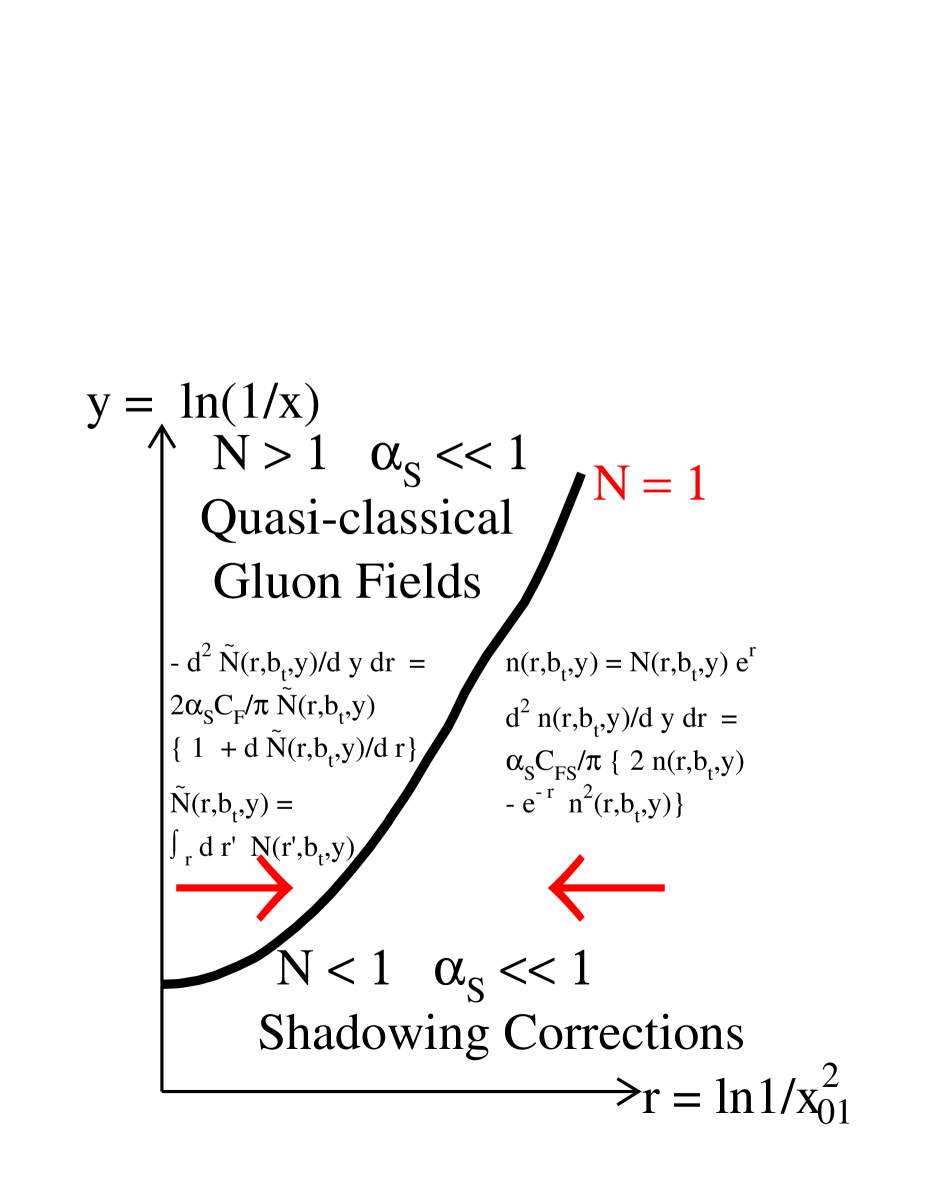
Figure 1: Different regions for the solution to the hdQCD evolution equation in the kinematic plot of DIS. The equation $N({\mathbf{x}},b_{t},y)\,=\,1$ gives the critical line.

2.2 The nonlinear equation for hdQCD evolution

Yu. Kovchegov in his proof [9], that the GLR equation is able to describe the whole kinematic region including very low values of $x$, uses heavily two principle ideas suggested by A. Mueller [10]:

• The QCD interaction at high energy does not change the transverse separation between quark and antiquark ( the colour dipole size ), and, therefore, colour dipoles can be considered as correct degrees of freedom at high energies which diagonalize the strong interaction matrix;

• The process of interaction of a dipole with the target has two clear stages:

  1. Decay of the dipole into two dipoles, which is described by

     $$|\Psi(\,{\mathbf{x_{01}}}\,\rightarrow\,{\mathbf{x_{02}}}\,\,+\,\,{\mathbf{x_{12}}}\,)|^{2}\,\,\,=\,\,\,\frac{{\mathbf{x^{2}_{01}}}}{{\mathbf{x^{2}_{02}}}\,{\mathbf{x^{2}_{12}}}}\,\,;$$ (2.7)

  2. Interaction of each dipole with the target with amplitude $N({\mathbf{x}},b_{t},y)$.

The equation is pictured in Fig.2 and it has the following analytic form:

$$\frac{dN({\mathbf{x_{01}}},b_{t},y)}{dy}\,\,\,=\,\,\,-\,\frac{2\,C_{F}\,\alpha_{S}}{\pi}\,\ln\left(\frac{{\mathbf{x^{2}_{01}}}}{\rho^{2}}\right)\,\,N({\mathbf{x}},b_{t},y)\,\,\,+\,\,\,\frac{C_{F}\,\alpha_{S}}{\pi}\,\,\int_{\rho}\,\,d^{2}{\mathbf{x_{2}}}\,\frac{{\mathbf{x^{2}_{01}}}}{{\mathbf{x^{2}_{02}}}\,{\mathbf{x^{2}_{12}}}}\,\,\times\,\,$$ (2.8)

$$\left(\,\,2\,N({\mathbf{x_{02}}},{\mathbf{b_{t}-\frac{1}{2}x_{12}}},y)\,\,\,-\,\,\,N({\mathbf{x_{02}}},{\mathbf{b_{t}-\frac{1}{2}x_{12}}},y)\,\,N({\mathbf{x_{12}}},{\mathbf{b_{t}-\frac{1}{2}x_{02}}},y)\,\,\right)\,\,.$$

Assuming that ${\mathbf{x_{12}}}$ and ${\mathbf{x_{20}}}$ are much smaller than the values of the typical impact parameter ( $b_{t}$ ), one can see that Eq. (2.8) is the GLR equation but in the space representation. It turns out that this representation is very convenient for searching solutions to Eq. (2.8).

Figure 2: Pictorial representation of the nonlinear evolution equation.

The first term in the r.h.s. of the equation gives the contribution of virtual corrections, which appear in the equation as a result of the normalization of the partonic wave function of the fast colour dipole ( see Ref. [10] ). The second term describes the decay of the colour dipole with the size ${\mathbf{x_{01}}}$ into two dipoles wth sizes ${\mathbf{x_{02}}}$ and ${\mathbf{x_{12}}}$ and their interactions with the target in the impulse approximation ( notice factor 2 in Eq. (2.8) ). The third term corresponds to simultaneous interaction of two produced colour dipoles with the target and describes the Glauber-type corrections for scattering of these dipoles.

Being differential equation, Eq. (2.8) needs an initial condition at $y=0$ to be solved. In Ref. [9]it was shown that the initial condition for $N({\mathbf{x_{01}}},b_{t},y)$ is the Mueller - Glauber formula [15], namely,

$$N({\mathbf{x_{01}}},b_{t},y=0)\,\,\,=\,\,\,2\,\,\left(\,\,1\,\,\,-\,\,\,\exp\{\,-\,\,\frac{\alpha_{S}\,\pi^{2}}{4\,N_{c}\,\pi\,R^{2}_{A}}\,{\mathbf{x^{2}_{01}}}\,A\,\,x_{0}G^{DGLAP}_{N}(x_{0},\frac{1}{{\mathbf{x^{2}_{01}}}})\,\,e^{-\frac{b^{2}_{t}}{R^{2}_{A}}}\}\,\,\right)\,\,;$$ (2.9)

where $x_{0}G^{DGLAP}_{N}(x_{0},\frac{1}{{\mathbf{x^{2}_{01}}}})$ is the gluon structure function obtained as a solution to the DGLAP linear evolution equations [8].

2.3 The strategy of searching for solutions

Eq. (2.8) is nonlinear integro-differential equation which is rather difficult to solve. However, this equation can be simplified and can be reduced to nonlinear but defferential equation in partial derivatives in two different kinematic regions (see Fig.1 ): to the right of the critical line ($r\,>\,r_{cr}$) and to the left of the critical line ($r\,<\,r_{cr}$).

2.3.1 $\mathbf{r\,\,>\,\,r_{cr}}$

Indeed, for $r\,>\,r_{cr}$, the size of the two produced colour dipoles ( ${\mathbf{x_{02}}}$ and ${\mathbf{x_{12}}}$ ) are much larger than the size of the initial colour dipole (${\mathbf{x_{01}}}$ ). Therefore, we can reduce the kernel of Eq. (2.8) to [9]

$$\int_{\rho}\,\,d^{2}{\mathbf{x_{2}}}\,\,\frac{{\mathbf{x^{2}_{01}}}}{{\mathbf{x^{2}_{02}}}\,{\mathbf{x^{2}_{12}}}}\,\,\,\longrightarrow\,\,\,{\mathbf{x^{2}_{01}}}\,\pi\,\,\int^{\frac{1}{\Lambda^{2}_{QCD}}}_{{\mathbf{x^{2}_{01}}}}\,\,\frac{d{\mathbf{x^{2}_{02}}}}{(\,{\mathbf{x^{2}_{02}}}\,)^{2}}\,\,.$$ (2.10)

Introducing a new function $n({\mathbf{x_{01}}},b_{t},y)\,\,=\,\,N({\mathbf{x_{01}}},b_{t},y)/{\mathbf{x^{2}_{01}}}$ and using the fact that the virtual corrections does not contribute in the double log approximation ( see Ref. [9] for example ), one can obtain the equation:

$$\frac{d^{2}n_{\rightarrow}(r,b_{t},y)}{dy\,\,d\,r}\,\,=\,\,\frac{\alpha_{S}\,C_{F}}{\pi}\,\,\{\,2\,n_{\rightarrow}(r,b_{t},y)\,\,\,-\,\,e^{-r}\,n^{2}_{\rightarrow}(r,b_{t},y)\,\}\,\,;$$ (2.11)

where $r\,=\,\ln(1/{\mathbf{x^{2}_{01}}})$.

In section 3 we will discuss the solution to this equation which satisfies the initial condition of Eq. (2.9).

2.3.2 $\mathbf{r\,\,<\,\,r_{cr}}$

As have been discussed many times ( see for example Ref. [13] and Ref. [14] ), the new scale appears in hdQCD which has a simple physical meaning of the average transverse momentum of parton in the parton cascade ( $Q_{cr}(x,b_{t})$ ). In this region the size of the initial colour dipole is larger than the typical size which we expect in hdQCD parton cascade ( ${\mathbf{x^{2}_{01}}}\,>$ $1/Q_{cr}(x,b_{t})$ ). Therefore, the main contribution in Eq. (2.8) comes from the configuration when one of the produced colour dipole has a size much smaller than the size of the initial colour dipole . We anticipate that the size of the smallest colour dipole will be of the order of $1/Q_{cr}(x,b_{t})$. Such a configuration simplify the kernel in Eq. (2.8) which has a form

$$\int_{1/Q_{cr}(x,b_{t})}\,\,d^{2}{\mathbf{x_{2}}}\,\,\frac{{\mathbf{x^{2}_{01}}}}{{\mathbf{x^{2}_{02}}}\,{\mathbf{x^{2}_{12}}}}\,\,\,\longrightarrow\,\,\,\,\pi\,\,\int^{{\mathbf{x^{2}_{01}}}}_{1/Q_{cr}(x,b_{t})}\,\,\frac{d{\mathbf{x^{2}_{02}}}}{{\mathbf{x^{2}_{02}}}\,}\,\,+\,\,\pi\,\,\int^{{\mathbf{x^{2}_{01}}}}_{1/Q_{cr}(x,b_{t})}\,\,\frac{d{\mathbf{x^{2}_{12}}}}{{\mathbf{x^{2}_{12}}\,}}\,\,;$$ (2.12)

The sum of two terms reflects the fact that two different produced colour dipoles can be small. In momentum representation Eq. (2.12) means that we sum $\log^{n}(Q^{2}_{cr}(x,b_{t})/Q^{2})$ which are the normal contributions for the DGLAP evolution coming from integration over transverse momentum from the small transverse momentum ($Q^{2}$ ) to the large one ( $Q^{2}_{cr}(x,b_{t})$ ).

Introducing a new function $\tilde{N}(r,b_{t},y)\,\,=\,\,\int_{r}\,dr^{\prime}N(r^{\prime},b_{t},y)$, we reduce Eq. (2.8) to the differential equation:

$$-\,\frac{d^{2}\tilde{N}_{\leftarrow}(r,b_{t},y)}{d\,y\,\,d\,r}\,\,\,=\,\,\,\frac{2\,\alpha_{S}\,C_{F}}{\pi}\,\,\{\,\tilde{N}_{\leftarrow}(r,b_{t},y)\,\,+\,\,{\tilde{N}}_{\leftarrow}(r,b_{t},y)\,\frac{d{\tilde{N}}_{\leftarrow}(r,b_{t},y)}{dr}\,\}\,\,.$$ (2.13)

One can see that in differential equation ( Eq. (2.13) ) we lost any dependence of the scale $Q_{cr}(x,b_{t})$ and it will come back to the problem only in matching a solution to Eq. (2.13) with a solution to Eq. (2.11).

In section 4 we will find a solution to this equation which match the solution of Eq. (2.11) on the critical line.

2.3.3 The general solution

Let us summarize what solution we are looking for:

1. We are going to solve the differential equation (see Eq. (2.11) ) to the right of the critical line which satisfies the initial condition given by the Mueller-Glauber formula (see Eq. (2.9);

2. We are going to find the solution to the differential equation ( see Eq. (2.13) ) to the left of the critical line;

3. We match the solution of Eq. (2.11) with the solution of Eq. (2.13) on the critical line;

4. We can hope that the solution of these two differential equations will be close to the solution to Eq. (2.8) in the vicinity of the critical line ($r\,\approx\,r_{cr}$)since we provide the matching of these two solutions on the critical line.

2.4 Experience of solving the GLR-type nonlinear equations

During the past two decades we have learned the main properties of the solution to the GLR-like nonlinear differential equations. Our experience in solution of these equations based on three different approaches that have been developed.

First, these equations were solved in semiclassical approximation, assuming $N=e^{S}$ where $S$ is a smooth function of $r$ and $y$, namely $d^{2}S/dydr\,\,\ll\,\,(dS/dy)^{2}$ or $(dS/dr)^{2}$ (see Refs. [1][16] [17][6] and references therein). In this approximation the GLR - type equation can be solved using characteristics method which leads to existence of a special ( critical ) line. All charecteristics in the region of low $x$ cannot cross this line but can approach it. The nonlinear term provides that the parton density $N(r,b_{t}=0,y)$ is constant on critical line. To the right of the critical line ( $r\,>\,r_{cr}$ ) the nonlinear corrections turns out to be small and the solution can be found as a solution of the linear DGLAP evolution equation but with the boundary conditions: $N=Const$ on the critical line. For our attempts to find a solution the important message from the semiclassical approach is the fact that we have a new scale ($Q_{cr}(x,b_{t})$ ) and the properties of the solution looks differently for $r>r_{cr}=\ln Q^{2}(x,b_{t})$ and for $r<r_{cr}$.

In Ref. [11] a new method was suggested for solving Eq. (2.11). The generating function was constructed which linearize Eq. (2.11) reducing Eq. (2.11) to a linear equation in partial derivatives but with one more variable. It is easy to find a general solution of this linear equation and all difficulties are concentrated in finding the solution which satisfies the boundary condition. We are going to use this method to find a solution to the right of the critical line.

In the region of very low $x$, a new idea for searching a solution of the GLR-type nonlinear equation was suggested in Ref.[12]. In this paper it was argued that the solution of Eq. (2.11), which satisfies all physics restrictions , is a function of one variable: $z=4\bar{\alpha}_{S}y\,-\,r$. We will find this solution in an explicit way in section 4 and will show how to match this solution with the solution to the right of the critical line.

2.5 Theory status of the equations

In this subsection we recall the main assumptions that have been made to obtain the nonlinear evolution equationsfor hdQCD (see Eq. (2.8), Eq. (2.11) and Eq. (2.13) ).

1. For derivation of all equations we used the leading log(1/$x$ ) approximation of pQCD. Only in this approximation we can neglect the energy recoiled during emission of the colour dipole ( the linear term in equations ) or during rescattring of this dipole ( the nonlinear term ). Formally speaking, we have to assume that parameter $\alpha_{S}\log(1/x)\,\,\geq\,\,1$ while $\alpha_{S}\,\,\ll\,\,1$;

2. To obtain the differential equations ( see Eq. (2.11) and Eq. (2.13) ) we have to assume existence of a more restricting parameter $\alpha_{S}ry\,\geq\,\,1$, but $\alpha_{S}r\leq 1$ and $\alpha_{S}y\leq 1$, which corresponds to the double log approximation of pQCD in the linear evolution equation;

3. The number of colours should be large ( $N_{c}\,\gg\,1$). It has been shown[18] that for $N_{c}\,\approx\,1$ the correlations between colour dipoles should be taken into account which break the simple physical picture of Fig.2. In the double log approximation these correlations can be taken into account [11] but they lead to rather complicated equations. On the other hand, in Ref. [11] it was demonstrated that all these complications lead to corrections of the order of $1/N^{2}_{c}$ and can be neglected even for $N_{c}$ = 3;

4. The master equation ( see Eq. (2.8) ) sums so called “fan” diagrams ( see Fig. 3a ), which reflect the fact that the fast colour dipole decays into two colour dipoles. However, the recombination of two colour dipoles into one have been omitted (see Fig. 3b). For $r>r_{cr}$ it has been proven that such diagrams give only small corrections [1] but in the kinematic region to the left of the critical line such enhanced diagrams can be neglected only in the case of scattering off the heavy nucleus. It turns out ( see Refs. [19] [6] [9] ) that in the case of heavy nucleus the contributions of “fan” diagrams are proportionsal to $\gamma A^{\frac{1}{3}}$ while enhanced diagrams of Fig.3b are of the order of $\gamma$ without large factor $A^{\frac{1}{3}}$. Therefore, our approach is valid only for heavy nuclei and can be considered only as a model for the interaction with a hadron;

5. We assume that (i) there are no correlations between different nucleons in a nucleus and (ii) the average $b_{t}$ for colour dipole - nucleon interaction is much smaller than $R_{A}$. Both these assumptions are usual for treatment of nucleus scattering.

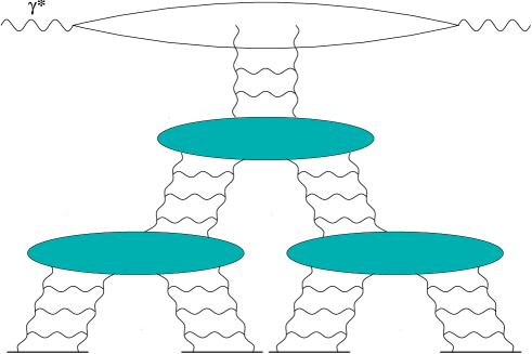
Fig. 3-a	Fig.3-b

Figure 3: “Fan” ( Fig. 3a ) and enhanced ( Fig. 3b ) diagrams.

3 Solution to the right of the critical line

In this kinematic region we use the generating function method, proposed in Ref. [11], which linearize Eq. (2.11). Following Ref. [11], we introduce a generating function

$$g_{A}(r,y,b_{t},\eta)\,\,\,=\,\,\,\sum^{\infty}_{n=1}\,\,\,\,n^{(n)}_{N,\rightarrow}(r,y,b_{t})\,e^{n\,\eta}\,\,,$$ (3.1)

where $n^{(1)}_{\rightarrow}\,=\,n_{\rightarrow}(r,y,b_{t})=N(r,b_{t},y)\,e^{r}\,=\,(\alpha_{S}\,\pi^{2}/2N_{c})\,\,\rho(r,b_{t},y)$ is proportional to the density of colour dipoles in the target. $n^{(n)}_{\rightarrow}$ is proportional to the probability to have $n$ - colour dipoles with the same size $e^{-r}$ in the parton cascade. In the case, when we neglect correlations between colour dipoles in the parton cascade, $n^{(n)}_{\rightarrow}\,\,=\,\,C_{n}(A)\left(\,n^{(1)}_{\rightarrow}\,\right)^{n}$. Coefficients $C_{n}(A)$ should be found from the initial condition of Eq. (2.9).

For $n^{(n)}_{\rightarrow}(r,b_{t},y)$ we can write the evolution equation of the Eq. (2.11) - type, noticing that every colour dipole with size $r$ at rapidity $y$ and impact parameter $b_{t}$ can either propagate to rapidity $y+dy$ changing its size from $r$ to $r+dr$ ( see first two terms in Fig.2 ) or decay into two colour dipoles ( see the last term in Fig. 2 and Fig. 3a). This observation leads to equation [11]

$$\frac{\partial^{2}n^{(n)}_{\rightarrow}(r,b_{t},y)}{\partial y\partial r}\,\,\,=\,\,\,\bar{\alpha}_{S}\,\{\,n^{2}\,\,n^{(n)}_{\rightarrow}(r,b_{t},y)\,\,\,-\,\,\,n\,\,e^{-r}\,\,n^{(n+1)}_{\rightarrow}(r,b_{t},y)\,\}\,\,,$$ (3.2)

where coefficient $\bar{\alpha}_{S}\,n^{2}$ corresponds to $\omega\,\gamma_{n}(\omega)$ where $\gamma_{n}$ is the anomalous dimension of $n^{(n)}_{\rightarrow}$ and $\omega$ is variable conjugated to $y$. In Refs.[20] the limit of small $\omega$ ( low $x$ ) for $\gamma_{n}$ has been calculated.

Comparing Eq. (3.1) with Eq. (2.9) one can obtain the following information on the generating function of Eq. (3.1):

$$C_{n}\,\,\,=\,\,\,\frac{(-1)^{n+1}}{2^{n}\,\,n!}\,\,;$$ (3.3)

$$N(r,b_{t},y)\,\,\,=\,\,\,2\,\,g_{A}\left(\,r,y,b_{t},\eta\,\,=\,\,-r\,+\,\eta_{A}\,\right)\,\,;$$ (3.4)

$$n^{(n)}_{N,\rightarrow}(r,y=0(x=x_{0}),b_{t})\,\,=\,\,C_{n}\left(\,n^{DGLAP}_{N,\rightarrow}(r,y=0(x=x_{0}),b_{t}\,\right)^{n}\,\,;$$ (3.5)

$$n^{DGLAP}_{N,\rightarrow}(r,y=0(x=x_{0}),b_{t})\,\,\,=\,\,\frac{\alpha_{S}\,\pi^{2}}{2N_{c}\pi R^{2}_{N}}\,\,\,\,x_{0}G_{N}(x_{0},e^{r})\,S_{N}(b_{t})\,\,;$$ (3.6)

$$\eta_{A}\,\,\,\,=\,\,\,\ln\left(\,A\,R^{2}_{N}\,S_{A}(b_{t})\,\right)\,\,\,.$$ (3.7)

Eq. (3.5) and Eq. (3.6) mean that we consider $x=x_{0}$ to be so small that we can neglect correlations between produced colour dipoles.

Eq. (3.2) can be rewritten as a linear equation for the generating function $g_{A}$ of Eq. (3.1):

$$\frac{\partial^{2}}{\partial y\partial r}g_{A}(r,y,b_{t},\eta,)\,\,\,=$$ (3.8)

$$\bar{\alpha}_{S}\frac{\partial^{2}}{\partial\eta^{2}}g_{A}(r,y,b_{t},\eta)\,\,-\,\,\bar{\alpha}_{S}\gamma e^{-r-\eta}\,\,\left(\,\frac{\partial g_{A}(r,y,b_{t},\eta)}{\partial\eta}-g_{A}(r,y,b_{t},\eta)\,\right)\,\,,$$

with $\gamma=1$.

This equation is a linear equation which can be solved just going to Mellin transform with respect to $y$ and $\xi=r+\eta$:

$$g_{A}(\xi,y,b_{t},\eta)=\int\frac{d\omega dp}{(2\pi i)^{2}}g_{A}(\xi,\omega,b_{t},p)\,e^{\omega y+p\eta}.$$ (3.9)

In Eq. (3.9) the contours of integration over $\omega$ and $p$ lie along the imaginary axis to the right of all singularities in $\omega$ and $p$.

Substituting Eq. (3.9) into Eq. (3.8) we obtain the following equation for the Mellin image $g_{A}(\xi,\omega,b_{t},p)$.

$$\frac{dg_{A}(\xi,\omega,b_{t},p)}{d\xi}\,\,\,=\,\,\frac{\bar{\alpha}_{S}}{\omega}\,\,\,\{\,\,p^{2}\,\,-\,\,\gamma\,(\,p-1\,)\,\,e^{-\xi}\,\,\}\,\,g_{A}(\xi,\omega,b_{t},p)\,\,,$$ (3.10)

which has an obvious solution:

$$g_{A}(\xi,\omega,b_{t},p)\,\,\,=\,\,g_{A}(\omega,p,b_{t})\,\,e^{\frac{\bar{\alpha}_{S}}{\omega}\,p^{2}\,\,\xi\,\,+\,\,\frac{\bar{\alpha}_{S}\,\gamma}{\omega}\,(p-1)\,\left(\,e^{-\xi}\,-\,e^{-\eta_{A}}\,\right)}\,\,.$$ (3.11)

Function $g_{A}(\omega,p,b_{t})$ should be found from the initial condition of Eq. (2.9) ( see also Eq. (3.3) - Eq. (3.6) ). Our statement is that

$$g_{A}(\omega,b_{t},p)\,\,\,=\,\,\,\Gamma(-f(p))\,\,\,\left(\frac{\alpha_{S}\pi^{2}}{4\pi R^{2}_{N}}\right)^{f}\,\,\frac{df(p)}{dp}e^{\frac{\bar{\alpha}_{S}\gamma}{\omega}\,(p-1)\,e^{-\eta_{A}}}\,\,e^{\frac{\bar{\alpha}_{S}}{\omega}\,p^{2}\,\,\eta_{A}}$$ (3.12)

satisfies initial conditions, with $f(p)=p\,\,+\,\,\frac{\bar{\alpha}_{S}\,p^{2}}{\omega}$. Substituting Eq. (3.12) in Eq. (3.11) and changing variables of integration from $p$ to $f$ ,we obtain

$$g_{A}(\xi,b_{t},y,\eta)=\int\frac{d\omega df}{(2\,\pi\,i)^{2}}\,\,\Gamma(-f)\,\,\left(\frac{\alpha_{S}\pi^{2}}{\pi R^{2}_{N}}\right)^{f}e^{-p(f)r\,+\,f\xi\,+\,f\eta_{A}+\omega y+\frac{\bar{\alpha}_{S}\gamma\,(p(f)-1)}{\omega}}\,\,,$$ (3.13)

where $p(f)$ is determined by

$$f\,\,=\,\,p(f)\,\,+\,\,\frac{\bar{\alpha}_{S}}{\omega}\,p^{2}(f)\,\,.$$ (3.14)

Indeed, at $y=y_{0}$ ( $x=x_{0}$ ) , $|\xi|\,\,\ll\,\,r$, $\xi=\eta_{A}$, $r\,\,\gg\,\,1$, we have

$$g_{A}(r,b_{t},y=y_{0},\eta=-r+\eta_{A}) = \int\frac{d\omega df}{(2\,\pi\,i)^{2}}\,\left(\frac{\alpha_{S}\pi^{2}}{4\,N_{c}\pi R^{2}_{N}}\right)^{f}\,\,\Gamma(-f)\,e^{-f\,r\,+\,f\,\eta_{A}\,\,+\,\,\omega\,y_{0}\,\,-\,\,\frac{\bar{\alpha}_{S}}{\omega}\,f^{2}}$$ (3.15)

$$= \sum_{n=1}^{\infty}\frac{(-1)^{n}}{n!}\,e^{-n\,r}\,\left(\frac{\alpha_{S}\pi^{2}}{N_{c}\pi R^{2}_{N}}\right)^{n}e^{n\eta_{A}}\,\int\frac{d\,\omega}{2\pi i}\,.\,e^{\omega y_{0}-\frac{\bar{\alpha}_{S}n^{2}r}{\omega}}\,\,$$

$$= \sum_{n=1}^{\infty}\frac{(-1)^{n}}{n!}\,\left(\,\frac{\alpha_{S}\pi^{2}}{\,4\,N_{c}\,\pi\,R^{2}_{A}}\,{\mathbf{x^{2}_{01}}}\,Ax_{0}G^{DGLAP}_{N}(x_{0},\frac{1}{{\mathbf{x^{2}_{01}}}})\,\right)^{n}\,\,.$$

Taking into account Eq. (3.4), one can see that Eq. (3.15) reproduces correctly the initial condition of Eq. (2.9).

It should be stressed that the contour of integration over $f$ was taken along positive real axis in such a way that all positive and integer $f$ are enveloped by it. The integral over $f$ is well defined due to rapid decrease of $\Gamma(-f)$ ( see Ref. [11] ). To study asymptotic behaviour of the parton densities at low $x$ we have to move the contour toward the imaginary axis. The asymptotic stems from the rightmost singularities in $f$ as well as from possible saddle points in this integral. The first dangerous region is a vicinity of $f\,\rightarrow\,1$ where we expect a saddle point. To investigate a situation near f$=1$, we introduce a new variable $f\,=\,1\,\,+\,\,t$, hoping that $t$ will be very small. At $t\,\rightarrow\,0$ our solution of Eq. (3.13) has a form

$$g_{A}(r,b,y,\eta=\eta_{A}+\tilde{\eta}) = \int\frac{d\omega df}{(2\pi i)^{2}}\Gamma(-f)e^{\frac{\bar{\alpha}_{S}\gamma}{\omega}(p-1)\,e^{-\eta_{A}}+f(\eta_{A}+\tilde{\eta})+pr+\omega y}$$ (3.16)

$$= \int\frac{d\omega\omega dt}{(2\pi i)^{2}t}e^{\psi(\omega,r,t,b_{t})}\,e^{\eta_{A}+\tilde{\eta}}\,\,,$$

where $\tilde{\eta}\,=\,\ln\left(\frac{\alpha_{S}\pi^{2}}{N_{c}\pi R^{2}_{N}}\right)$.

In Appendix A we calculate the integral of Eq. (3.16) using the saddle point approximation and the answer, that we obtain in this appendix ( see Eq. (A.5) ) can be written in the form:

$$g_{A,\rightarrow}(y,\xi=\eta_{A},r,b_{t})\,=\,\frac{\omega^{2}_{cr}}{2\pi\,2\bar{\alpha}_{S}(r)\,t_{0}\,\varsigma}\,\frac{\alpha_{S}\pi^{2}A}{4\pi\,R^{2}_{A}}\,e^{-\frac{b^{2}_{t}}{R^{2}_{A}}}\,e^{\omega_{cr}y-r+\frac{\bar{\alpha}_{S}r}{\omega_{cr}}}\,\,,$$ (3.17)

with $\omega_{cr}$ is given by Eq. (A.3) and $t_{0}$ by Eq. (A.4).

One can see that Eq. (3.17) leads to $g_{A}(y,\xi=\eta_{A},r,b_{t})$ which is constant on the critical line given by equation:

$$\tilde{\Psi}\,\,=\,\,\omega_{cr}\,y_{cr}\,\,-\,\,r\,\,+\,\,\frac{\bar{\alpha}_{S}}{\omega_{cr}}\,r\,\,+\,\,\eta_{A}\,+\,\tilde{\eta}\,\,-\,\,\ln\frac{2\bar{\alpha}_{S}\,\varsigma\,r\,t_{0}}{\omega_{cr}}\,\,\,=\,\,Const(\alpha_{S})$$ (3.18)

where $Const(\alpha_{S})$ can be a function of $\alpha_{S}$ but it does not depend on neither $y$ nor $r$ or $\eta_{A}$. We anticipate that the value of $t_{0}$ will be small on the critical line and, because of this, the last term in Eq. (3.18) has been taken into account in the phase $\tilde{\Psi}$.

The solution of Eq. (3.18) gives

$$y_{cr}\,\,=\,\,\frac{1}{4\bar{\alpha}_{S}}\,\left(\,r\,\,-\,\,2(\eta_{A}\,+\,\tilde{\eta})\,\,+\,\,2\,\right)\,\,.$$ (3.19)

This line gives the minimal value for $\tilde{\Psi}$, namely, $\tilde{\Psi}\,=\,1$.

The value of $g_{A}(y,\xi=\eta_{A},r,b_{t})$ is equal to

$$g_{A,cr}(y,\xi=\eta_{A},r,b_{t})\,\,\,=\,\,\,\frac{e\,\,\bar{\alpha}_{S}}{\pi}.$$ (3.20)

Solving Eq. (3.19) with respect to $r$ we obtain the typical momentum ( colour dipole size ) on the critical line

$$Q^{2}_{cr}(x;b_{t})\,\,=\,\,Q_{0}^{2}\left(\frac{\alpha_{S}}{N_{c}R^{2}_{N}\mathbf{e}}\right)^{2}\,\,\left(\frac{AR^{2}_{N}}{R^{2}_{A}}\right)^{2}\,\,e^{4\bar{\alpha}_{S}y}\,\,e^{-\frac{2b^{2}_{t}}{R^{2}_{A}}}.$$ (3.21)

At $b_{t}=0$ $Q^{2}_{cr}(x;b_{t}=0)\,\,\propto\,\,A^{\frac{2}{3}}$, as can be see easily from Eq. (3.21).

Comparing Eq. (3.20) with Eq. (2.4) one sees that $xG_{A}(x,\frac{1}{{\mathbf{x^{2}}}})$ on the critical line is equal to

$$xG_{A,cr}(x,\frac{1}{{\mathbf{x^{2}}}})\,\,\,=\,\,\,\frac{2N_{c}\pi R^{2}_{A}Q^{2}_{cr}}{\alpha_{S}\pi^{2}}\,N({\mathbf{x^{2}}},b_{t}=0,y_{cr})\,\,=\,\,{\frac{4N_{c}^{2}e}{\pi^{3}}}\,R^{2}_{A}\,Q^{2}_{cr}(x)\,\,\propto\,\,A^{\frac{4}{3}}\,\,.$$ (3.22)

It is interesting to notice that such A-dependence can be understood directly from the Mueller - Glauber formula of Eq. (2.9). Indeed, the shadowing corrections become to be essential when

$$\frac{\alpha_{S}\pi^{2}}{4N_{c}\pi R^{2}_{A}}{\mathbf{x^{2}}}\,AxG(x,1/{\mathbf{x^{2}}})\,\,\approx\,\,1\,\,.$$ (3.23)

Recalling that anomalous dimension in the vicinity of the critical line is equal to $\gamma(\omega)=\frac{\bar{\alpha}_{S}}{\omega_{cr}}\,=\,\frac{1}{2}$, one can find from Eq. (3.23) that ${\mathbf{x^{2}_{cr}}}\,\,=\,\,1/Q^{2}_{cr}\,\,\propto\,\,A^{-\frac{2}{3}}$, which is the same A-dependence that we obtained from more advanced calculations ( see Eq. (3.22) ).

4 Solution to the left of the critical line

In this section we are going to solve Eq. (2.13) using the idea suggested in Ref. [12], namely, $\tilde{N}_{\leftarrow}\,\,=\,\,\tilde{N}_{\leftarrow}(z)$ where

$$z\,\,\,=\,\,\,4\,\bar{\alpha}_{S}\,\,y\,\,\,-\,\,\,r\,\,-\,\,\beta(A;b_{t})\,\,.$$ (4.1)

Function $\beta(A;b_{t})$ can be chosen in a such way that the equation for the critical line in terms of new variable $z$ looks as $z=0$. One can see from Eq. (3.19) that $\beta(b_{t})$ is equal to

$$\beta(b_{t})\,\,\,=\,\,\,-2\tilde{\eta}\,\,-\,\,2\,\ln\frac{A\,R^{2}_{N}}{\pi R^{2}_{A}}\,\,+\,\,\frac{2b^{2}_{t}}{R^{2}_{A}}\,\,+\,\,2\,\,.$$ (4.2)

Assuming that $\tilde{N}_{\leftarrow}(r,b_{t},y)$ is a function of $z$ and $b_{t}$ only, we can rewrite Eq. (2.13) in the form:

$$\frac{d^{2}\tilde{N}_{\leftarrow}(z,b_{t})}{dz^{2}}\,\,\,=\,\,\frac{1}{4}\,\,\left(\,1\,\,\,-\,\,\,\frac{d\tilde{N}_{\leftarrow}(z,b_{t})}{dz}\,\right)\,\,\tilde{N}_{\leftarrow}(z,b_{t})\,\,.$$ (4.3)

Here we used the explicit equation for variable $z$, namely, $z=4\bar{\alpha}_{S}y-r-\beta(b_{t})$.

4.1 A solution to Eq. (4.3)

First, we find a solution to Eq. (4.3) introducing function $\zeta(z)$ in the following way:

$$\tilde{N}_{\leftarrow}(z,b_{t})\,\,=\,\,\int^{z}\,\,dz^{\prime}\,\left(\,1\,\,-\,\,e^{-\zeta(z,b_{t})}\,\right)\,\,.$$ (4.4)

For function $\zeta(z)$ Eq. (4.3) can be reduced to

$$\frac{d\zeta(z,b_{t})}{dz}\,\,\,=\,\,\,\frac{1}{4}\,\,\int^{z}\,\,dz^{\prime}\,\,\left(\,1\,\,-\,\,e^{-\zeta(z^{\prime},b_{t})}\,\right)\,\,.$$ (4.5)

Changing variable in the integral from $z^{\prime}$ to $\zeta^{\prime}$ we have

$$\frac{d\zeta(z,b_{t})}{dz}\,\,\,=\,\,\,\frac{1}{4}\,\,\int^{\zeta}_{\zeta_{0}(b_{t})}\,\,\frac{d\zeta^{\prime}}{\frac{d\zeta^{\prime}}{dz^{\prime}}}\,\left(\,1\,\,-\,\,e^{-\zeta^{\prime}}\,\right)\,\,.$$ (4.6)

Eq. (4.6) can be easily solved and the solution is

$$z\,\,=\,\,\sqrt{2}\,\int^{\zeta}_{\zeta_{0}(b_{t})}\,\,\frac{d\zeta^{\prime}}{\sqrt{\zeta^{\prime}\,\,+\,\,\,(\,e^{-\zeta^{\prime}}\,\,-\,\,1\,)}}\,\,.$$ (4.7)

The numerical solution to Eq. (4.7) is given in Fig.4. This solution depends on the initial conditions on the critical line . There are two of them, namely,

$$N_{\leftarrow}(z=0)=N_{\rightarrow}(z=0)\,\,;$$ (4.8)

$$\frac{d\ln N_{\leftarrow}}{dz}|_{z=0}\,\,=\,\,\frac{d\ln N_{\rightarrow}}{dz}|_{z=0}\,\,=\,\,\frac{1}{2}\,\,.$$ (4.9)

We can assume that $\zeta\,\,\gg\,\,1$ at large $z$. In this case we can neglect $e^{-\zeta^{\prime}}$ in the integrand and we obtain an explicit analytic solution:

$$\zeta(z)\,\,=\,\,(\,\sqrt{\zeta_{0}(b_{t})}\,\,+\,\,\frac{z}{2\sqrt{2}}\,)^{2}\,\,,$$ (4.10)

or in terms $N(z,b_{t})$ we have

$$N_{\leftarrow}(z,b_{t})\,\,\,=\,\,\,1\,\,\,-\,\,\,\,e^{-\,\,(\,\sqrt{\zeta_{0}(b_{t})}\,\,+\,\,\frac{z}{2\sqrt{2}}\,)^{2}}\,\,\,$$ (4.11)

where $z_{0}(b_{t})$ should be found from matching of this solution with the solution of the previous section on the critical line.

4.2 Matching with the solution to the right of the critical line

We cannot use the simple solution of Eq. (4.10) for matching with the solution of Eq. (3.17) since $\zeta$ is expected to be rather small in the vicinity of the critical line and, therefore, we cannot neglect $e^{-\zeta}$ in Eq. (4.7). However, for small $\zeta\,\,\ll\,\,1$ we easily obtain a simple solution to Eq. (4.7), namely,

$$\ln\frac{\zeta}{\zeta_{0}(b_{t})}\,\,=\,\,\frac{1}{2}\,z\,\,.$$ (4.12)

Eq. (4.12) leads to Eq. (4.9) of matching condition. This equation allows us to find $\zeta_{0}(b_{t})$, namely,

$$1\,\,-\,\,e^{-\zeta_{0}(b_{t})}\,\,=\,\,N_{cr,\rightarrow}\,\,.$$ (4.13)

Eq. (4.12) and Eq. (4.13) provide matching as well as determine the parameters of the asymptotic behaviour for $N_{\leftarrow}$ given by Eq. (4.11). Using Eq. (3.20) one can find from Eq. (4.13) that

$$\zeta_{0}(b_{t})\,\,=\,\,2\,\frac{e\,\bar{\alpha}_{S}}{\pi}\,\,.$$ (4.14)

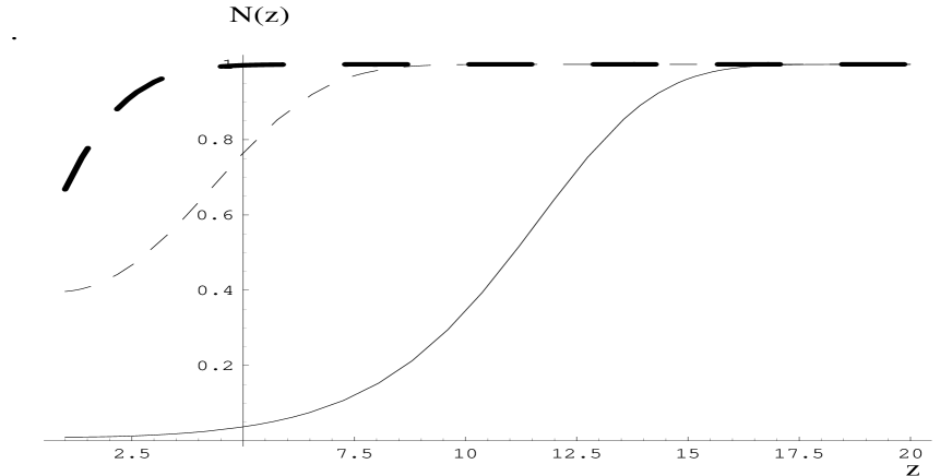
Figure 4: Dipole number density $N(z)$ as a function of the critical line parameter $z$. Solid line is the numerical solution with $\tilde{N}^{\prime}(0)=0.01$, while dashed line corresponds to $\tilde{N}^{\prime}(0)=0.4$. The bold dashed line shows the asymptotic solution of Eq. (4.11) with $\tilde{N}^{\prime}(0)=0.4$.

Fig.4 illustrates the behaviour of $N(z)$ versus $z$. One can see that asymptotic is reached only at very large $z\approx\,7-10$ or for very low $x$ ( $x\,\approx\,10^{-6}-10^{-7}$ ). At HERA we have $z\,\approx\,4-5$ and we are far away from the asymptotic solution. However, we can penetrate the region of large $z$ using a nuclear target,as one can see in Eq. (3.19). Indeed, for heavy nuclei we can easily have $2\eta_{A}\,\approx\,3.5-4$ . It gives a possibility to have even at HERA kinematic region sufficiently large values of $z\,\approx\,7.5-9$.

4.3 Stability of the solution

Arguments of the last section show, that the solution given by Eq. (4.7) has a big chance to be the solution to our equation. To prove this statement we need only to show that the solution of Eq. (4.7) is stable with respect to small perturbations of the initial conditions on the critical line. In other words, let us consider a small variation of the initial conditions $|\delta\zeta_{cr}(y,r,b_{t})|\,<\,\delta$ where $0<\,\delta\,\ll\,1$. The solution is stable if for every $\delta$ we can found a small $\epsilon$ such that $\epsilon\,\,\rightarrow\,\,0$ at $\delta\,\,\rightarrow\,\,0$. We can find a linear equation for function $\delta\zeta(y,r,b_{t})$ substituting $\zeta(y,r,b_{t})\,\,\longrightarrow\,\,\zeta_{s}\,\,\,+\,\,\,\delta\zeta(y,r,b_{t})$ where $\zeta_{s}$ is given by Eq. (4.7). Assuming that $\delta\zeta_{cr}(y,r,b_{t})$ is small we obtain a linear equation

$$\frac{\partial^{2}\delta\zeta(y,r,b_{t})}{\partial\,y\,\,\partial r}\,\,=\,\,\bar{\alpha}_{S}\,\,\delta\zeta(y,r,b_{t})\,\,e^{-\zeta_{s}(z)}\,\,.$$ (4.15)

In variables $z$ and $r$ this equation has a form

$$\frac{\partial^{2}\delta\zeta(z,r,b_{t})}{\partial\,z\,\,\partial r}\,\,=\,\,\frac{1}{4}\,\,\delta\zeta(z,r,b_{t})\,\,e^{-\zeta_{s}(z)}\,\,,$$ (4.16)

which can be solved going to Mellin transform with respect to variable $r$. Indeed, for Mellin image we have

$$\frac{d\delta\zeta(z,\nu,b_{t})}{d\,z}\,\,=\,\,\frac{1}{4\,\nu}\,\,\delta\zeta(z,\nu,b_{t})\,\,e^{-\zeta_{s}(z)}\,\,.$$ (4.17)

The general solution of Eq. (4.17) looks as follows

$$\delta\zeta(z,\nu,b_{t})\,\,\,=\,\,\int^{a+i\infty}_{a-i\infty}\,\,\frac{d\nu}{2\,\pi\,i}\,\delta\zeta(\nu)e^{\nu r\,\,+\,\,\frac{1}{\nu}\,\int^{z}_{0}\,dz^{\prime}\,\,e^{-\zeta_{s}(z^{\prime},b_{t})}}\,\,.$$ (4.18)

The integral over $z^{\prime}$ in Eq. (4.18) does not depend on $z$ at large $z$. It means that the solution given by this equation is actually the function of $r$ only. It is obvious that such a solution cannot be tolerated by the initial conditions on the critical line.

4.4 Low $\mathbf{x}$ ( high energy ) asymptotic

As we have discussed the total dipole cross section is equal to

$$\sigma_{dipole}\,\,=$$ (4.19)

$$\int\,d^{2}b_{t}\,2N(r,y,b_{t})\,\,\,=\,\,2\pi\,\{\int^{b^{2}_{0}}_{0}db^{2}_{t}\,\,N_{\leftarrow}\,\,+\,\,\int^{\infty}_{b^{2}_{0}}\,\,db^{2}_{t}\,\,N_{\rightarrow}\,\,\}=\,\,2\pi\int^{b^{2}_{0}}_{0}\,db^{2}_{t}\,\,=\,\,2\pi\,b^{2}_{0}(y,r)$$

since $N_{\leftarrow}(r,y,b_{t})\,\,\longrightarrow\,\,\,1$ at low $x$ ( see Eq. (4.11) ) and $N_{\rightarrow}(t,y,b_{t})$ gives a small contribution to the integral in Eq. (4.19).

The value for $b^{2}_{0}(y,r)$ we can evaluate recalling that solution of Eq. (4.11) is written for $z=4\,\bar{\alpha}_{S}\,y-r+2\tilde{\eta}+2\ln\frac{AR^{2}_{n}}{R^{2}_{A}}\,-\,\frac{2b^{2}_{t}}{R^{2}_{A}}\,\,>\,\,0$. Therefore,

$$b^{2}_{0}(y,r)\,\,=\,\,\frac{R^{2}_{A}}{2}\,\,\left(\,4\,\bar{\alpha}_{S}\,y-r\,+\,2\ln\frac{AR^{2}_{N}}{R^{2}_{A}}\,\right)\,\,,$$ (4.20)

which gives

$$\sigma_{dipole}\,\,\,=\,\,\,\pi\,R^{2}_{A}\,\left(\,4\,\bar{\alpha}_{S}\,y-r\,+\,2\,\ln\frac{AR^{2}_{N}}{R^{2}_{A}}\right)\,\,.$$ (4.21)

For the gluon structure function Eq. (4.21) leads to

$$xG(x,Q^{2})\,\,\,\longrightarrow\,\,Q^{2}\,R^{2}_{A}\,\,\left(\,4\,\bar{\alpha}_{S}\,\ln(1/x)\,\,-\,\,\ln Q^{2}\,+\,2\,\ln\frac{AR^{2}_{N}}{R^{2}_{A}}\right)\,\,.$$ (4.22)

Eq. (4.19) can be rewritten as an integral over $z$, namely

$$\sigma_{dipole}\,\, = \int\,d^{2}b_{t}\,2N(r,y,b_{t})\,\,\,=\,\,2\pi\,\{\int^{b^{2}_{0}}_{0}db^{2}_{t}\,\,N_{\leftarrow}\,\,+\,\,\int^{\infty}_{b^{2}_{0}}\,\,db^{2}_{t}\,\,N_{\rightarrow}\}\,\,;$$ (4.23)

$$= \,\,\pi\,R^{2}_{A}\,\int^{4\bar{\alpha}_{S}\,y\,-\,r\,+\,2\ln\frac{AR^{2}_{N}}{R^{2}_{A}}}_{0}\,d\,z\,\left(\,1\,\,-\,\,e^{-\,\zeta(z)}\,\right)\,\,+\,\,2\,\bar{\alpha}_{S}\,e\,R^{2}_{A}\,\,.$$ (4.24)

It is interesting to notice that $\sigma^{A}_{dipole}$ for nucleus target manifests itself a remarkable scaling in the kinematic region to the left of the critical line. Indeed, from Eq. (4.24) one can conclude that

$$\frac{\sigma^{A}_{dipole}}{\pi R^{2}_{A}}\,\,=\,\,\frac{\sigma^{N}_{dipole}\left(\,x_{B},\frac{Q^{2}\,(R^{2}_{A})^{2}}{A^{2}\,(R^{2}_{N})^{2}}\,\right)}{\pi R^{2}_{N}}\,\,.$$ (4.25)

Fig.5 shows the $Q^{2}$ behaviour of the ratio $\frac{\sigma^{A}_{dipole}}{\pi R^{2}_{A}}$ at $x=10^{-4}$ with $y=\ln(0.01/x)$ for different nuclei. The full line describes the nucleon target and other lines correspond to nuclei with A= 40 (Ca), 150, 296 (gold) going from bottom to the top. One can see that the cross sections are quite larger than the geometrical estimates.

Figure 5: The ratio of the dipole cross section to the geometrical estimates $\frac{\sigma^{A}_{dipole}}{\pi R^{2}_{A}}$ for low $x=10^{-4}$ ( $y=\ln(0.01/x)$ ) as a function of $Q^{2}$ for different nuclei. All other curves correspond to A=40, 150, 300 going from the bottom to the top; $\alpha_{S}=0.25,Q^{2}_{0}=1\,GeV^{2}$ .

It should be stressed that Eq. (4.20) is an artifact of the oversimplified Gaussian parameterization for the nucleus profile function ( see Eq. (2.6). In more realistic approach to the nucleus profile function ( for example the Wood-Saxon one [21] ) instead of $\exp(-b^{2}_{t}/R^{2}_{A})$ in Eq. (2.6) we have a function which is equal to 1 for $b_{t}\leq R_{A}$ and falls down as $\exp(-b_{t}/h)$, where $h$ does not depend on $A$, at $b_{t}>R_{A}$. Such function gives $b_{0}(y,r)$

$$b_{0}(y,r)\,\,=\,\,R_{A}\,\,+\,\,\frac{h}{2}\,\,\left(\,4\,\bar{\alpha}_{S}\,y-r\,+\,2\ln\frac{AR^{2}_{N}}{R^{2}_{A}}\,\right)\,\,,$$ (4.26)

instead of Eq. (4.20).

Therefore, we expect the following asymptotic behaviour for $\sigma_{dipole}$ and $xG(x,Q^{2})$

$$\sigma_{dipole} \rightarrow 2\,\pi\left(R\,\,+\,\,\frac{h}{2}\,\{\,4\,\bar{\alpha}_{S}\,y\,-\,r\,+2\ln\frac{AR^{2}_{N}}{R^{2}_{A}}\,\}\,\right)^{2};$$ (4.27)

$$xG(x,Q^{2}) \rightarrow Q^{2}\,\left(R\,\,+\,\,\frac{h}{2}\,\{\,4\,\bar{\alpha}_{S}\,y\,-\,r\,+2\ln\frac{AR^{2}_{N}}{R^{2}_{A}}\,\}\,\right)^{2}.$$ (4.28)

5 Summary

In this paper we found the solution to the evolution equation for high parton density QCD ( see Eq. (2.8) ). This solution is given by two equations: Eq. (3.13) to the right of the critical line ( see Fig.1) and Eq. (4.4) to the left of the critical line described by Eq. (3.19).

This solution gives the colour dipole density ($\rho=xG_{A}(x,\frac{1}{{\mathbf{x^{2}}}})/\pi R^{2}_{A}$ ) which is small to the right of the critical line , reaches the value of the order of unity on the critical line and increases up to the value $\rho\,\approx\,\,1/\alpha_{S}$ at very small values of $x$.

Such a behaviour of $\rho$ reveals itself in the following properties of the gluon structure function:

1. To the right of the critical line $xG$ is given by the DGLAP evolution equations;

2. On the critical line $xG(x,Q^{2}_{cr}(x))\,=\,Q^{2}_{cr}(x)R^{2}_{A}$ (see Eq. (3.22) ) where $,Q^{2}_{cr}(x)$ is defined by Eq. (3.21);

3. To the left of the critical line $xG(x,Q^{2})=Q^{2}\,R^{2}_{A}(4\bar{\alpha}_{S}y-r+2\ln\frac{AR^{2}_{N}}{R^{2}_{A}})$.

As far as A-dependence is concerned, in the kinematic region to the right of the critical line we have $xG_{A}\,\propto\,AxG_{N}$, while on the critical line $xG_{A}(x,Q^{2}_{cr}(x))\,\propto\,A^{\frac{4}{3}}$ and only to the left of the critical line we have $xG_{A}\,\,\propto\,\,Q^{2}R^{2}_{A}\,\,\propto\,\,A^{\frac{2}{3}}$.

Our solution reproduces the saturation of the gluon density but due to sufficiently mild dependence on the impact parameter the saturation leads to the dipole-target total cross section proportional to $\ln(1/x)$ in the region of the extremely low $x$ (see Eq. (4.21) for the exact answer).

Both the exact solution near the saturation limit (see Eq. (4.11) ) and the proportionality to $xG\,\propto\,Q^{2}R^{2}_{A}$ ( see Eq. (4.22) ) are the manifestation of the fact that nonlinear equation leads to the parton distribution which peaks at the size ${\mathbf{x^{2}}}\,\approx\,1/Q^{2}_{cr}(x)$. In other words, in the region of low $x$ the parton distribution has a definite mean transverse momentum, namely, $<p^{2}_{t}>=Q^{2}_{cr}(x)$. Therefore, this solution supports the more intuitive approach that has been discussed before for the parton distribution at low $x$ [13] [14].

We want also to draw your attention to the fact that in the region of small $x$ our solution leads to a new scaling between DIS with nucleon and DIS with nucleus given by Eq. (4.25). This equation allows us to calculate how nucleus DIS approaches $A^{\frac{2}{3}}$ dependence in the region of low $x$.

We hope, that our solution will stimulate a more detailed study of the properties of the high density parton system and, in particular, it will lead to more quantitive development of ideas suggested in Ref[14].

Appendix A Appendix

In this appendix we calculate the phase $\psi(\omega,r,t,b_{t})$ in Eq. (3.16) at $t\,\ll\,1$. Using Eq. (3.14), we can find $p$ for $\alpha_{S}\,\ll\,1$ and $t\,\rightarrow\,0$

$$p\,=\,1\,+\,t\,\,-\,\,\frac{\bar{\alpha}_{S}}{\omega}\,(1+2t)\,\,,$$ (A.1)

which leads to

$$\psi(\omega,r,t,b_{t}) + t(\eta_{A}+\tilde{\eta})=\frac{\bar{\alpha}_{S}\gamma}{\omega}\,e^{-\eta_{A}}(p-1)+pr+\omega y+t(\eta_{A}+\tilde{\eta})$$ (A.2)

$$\approx \omega y+r-\frac{\bar{\alpha}_{S}}{\omega}r-tr\left(\frac{\bar{\alpha}_{S}\gamma}{\omega(-r)}\,e^{-\eta_{A}}\,\,-\,\,1\,\,+\,\,\frac{2\bar{\alpha}_{S}}{\omega}+\frac{1}{r}(\eta_{A}+\tilde{\eta})\,\right)\,\,.$$

Integration over $t$ gives a $\delta$ - function which defines the value of $\omega=\omega_{cr}$.

$$\omega_{cr}\,=\,\frac{2\bar{\alpha}_{S}+\frac{\bar{\alpha}_{S}\gamma}{r}\,e^{-\eta_{A}}}{1-\frac{1}{r}(\eta_{A}+\tilde{\eta})}\,\,=\,\,\frac{2\,\bar{\alpha}_{S}\,\,\varsigma}{1-\frac{1}{r}(\eta_{A}+\tilde{\eta})}\,\,,$$ (A.3)

where $\varsigma\,=\,1+\frac{\gamma}{2\,r}e^{-\eta_{A}}$.

We can make the integration over $\omega=\omega_{cr}+\Delta$ , considering $\frac{\Delta}{\omega_{cr}}\,\,\ll\,\,1$.

$$\psi(\omega,r,t,b_{t})\,$$ (A.4)

$$\approx -r+\frac{\bar{\alpha}_{S}r}{\omega_{cr}}+\omega_{cr}y+\Delta\left(y-\frac{\bar{\alpha}_{S}r}{\omega_{cr}^{2}}-\frac{2\bar{\alpha}_{S}tr}{\omega_{cr}^{2}}\right)$$

$$= -r+\frac{\bar{\alpha}_{S}r}{\omega_{cr}}+\omega_{cr}y+\Delta\frac{2\bar{\alpha}_{S}(r)}{\omega_{cr}^{2}}\left(\underbrace{(y-\frac{\bar{\alpha}_{S}r}{\omega_{cr}^{2}})\frac{\omega_{cr}^{2}}{2\bar{\alpha}_{S}(r)\,\varsigma}}_{t_{0}}-t\right)\,\,.$$

Integration over $\Delta$ gives $\delta\left[\frac{2\bar{\alpha}_{S}(-r)}{\omega_{cr}^{2}}(t-t_{0})\right]$ which yields

$$g_{A}(y,\xi=\eta_{A},r,b_{t})\,=\,\frac{\omega^{2}_{cr}}{2\pi\,2\bar{\alpha}_{S}(r)\,t_{0}\,\varsigma}\,\frac{\alpha_{S}\pi^{2}A}{4\pi\,R^{2}_{A}}\,e^{-\frac{b^{2}_{t}}{R^{2}_{A}}}\,e^{\omega_{cr}y-r+\frac{\bar{\alpha}_{S}r}{\omega_{cr}}}\,\,.$$ (A.5)

References

- [1] L. V. Gribov, E. M. Levin and M. G. Ryskin, Phys.Rep. 100, 1 (1983).
-
[2]
A.H. Mueller and J. Qiu, Nucl. Phys. B268, 427 (1986);
E. Laenen and E. Levin, Ann. Rev. Nucl. Part. 44 (1994) 199 and references therein;
A.H. Mueller, Nucl. Phys. B437 (1995) 107;
G. Salam, Nucl. Phys. B461 (1996) 512;
A.L. Ayala, M.B. Gay Ducati and E.M. Levin, Nucl. Phys. B493, (1997) 305,B510,(1998) 355. -
[3]
L. McLerran and R. Venugopalan, Phys. Rev. D49 (1994)
2233,3352, D50 (1994) 2225, D53 (1996) 458;
J. Jalilian-Marian, A. Kovner, A. Leonidov and H. Weigert, Phys. Rev. D 59 (1999) 014014, 034007; Nucl. Phys. B504 (1997) 415;
J.Jalilian-Marian, A. Kovner, L. McLerran and H. Weigert, Phys. Rev. D55, (1997) 5414;
A. Kovner, L. McLerran and H. Weigert, Phys. Rev. D 52 (1995) 3809,6231 ; Yu. Kovchegov, Phys. Rev. D54, (996) 5463 , D55, (1997) 5445;
Yu. V. Kovchegov and A.H. Mueller, Nucl. Phys. B529 (1998) 451;
Yu. V. Kovchegov, A.H. Mueller and S. Wallon, Nucl. Phys. B507 (1997) 367. -
[4]
A.M. Cooper-Sarkar, R.C.E. Devenish and A. De
Roeck, Int.J.Mod.Phys. A13 (1998) 3385;
H.Abramowicz and A. Caldwell, hep-ex/9903037, Rev. Mod. Phys. ( in press ). -
[5]
E. Gotsman,E. Levin and U. Maor, Phys. Lett B379 (1996) 186;
B430 (1997) 120; Nucl. Phys. B464 (1996) 251; B493
(1997) 354;
A.H. Mueller, plenary talk at DIS’98 eds. Ch. Coremans and R. Roosen, WS, 1998; CU-TP-937-99, hep-ph/9904404;
E. Gotsman, E. Levin, U. Maor and E. Naftali, Nucl. Phys. B539 (1999) 535;
K. Golec-Biernat and M. Wüsthoff, Phys. Rev. D59 (1999) 014017, DTP-99-20,hep-ph/9903358. - [6] A.L. Ayala, M.B. Gay Ducati and E.M. Levin, Nucl. Phys. B493 (1997) 305,B510 (1998) 355.
- [7] J. Jalilian-Marian, A. Kovner, A. Leonidov and H. Weigert, Phys. Rev. D 59 (1999) 014014,Erratum- Phys. Rev. D59 (1999) 034007;
-
[8]
V.N. Gribov and L.N. Lipatov,Sov. J. Nucl. Phys. 15 (1972) 438
L.N. Lipatov, Yad. Fiz. 20(1974) 181 ;
G. Altarelli and G. Parisi, Nucl. Phys. B126 (1977) 298;
Yu.L. Dokshitser, Sov. Phys. JETP 46(1977) 641. - [9] Yuri V. Kovchegov, NUC-MN-99/1-T,hep-ph/9901281.
- [10] A.H. Mueller, Nucl. Phys. B425 (1994) 471.
- [11] E. Laenen and E. Levin, Nucl. Phys. B451 (1995) 207.
- [12] J. Bartels and E. Levin, Nucl. Phys. B387 (1992) 617.
- [13] E.M. Levin and M.G. Ryskin, Phys. Rept. 189 (1990) 267.
- [14] A.H. Mueller, CU - TP - 941, hep-ph/9906322, CU - TP - 937, hep-ph/9904404,
- [15] A. H. Mueller: Nucl. Phys. B335 (1990) 115.
- [16] J. Bartels, J. Blumlein and G. Shuler, Z. Phys.C50 (1991) 91.
- [17] J.C. Collins and J. Kwiecinski, Nucl. Phys. B335 (1990) 89.
-
[18]
J. Bartels, Phys. Lett. B298 (1993) 204, Z. Phys. C60 (1993) 471;
E. Levin, M. G. Ryskin and A.G. Shuvaev, Nucl. Phys. B387 (1992) 589. - [19] A. Schwimmer, Nucl. Phys. B94 (1975) 445.
- [20] E. Laenen, E. Levin and A.G. Shuvaev, Nucl. Phys. B419 (1994) 38.
- [21] C.W. De Jagier, H De Vries and C. De Vries, Atomic data and nuclear data tables 14 (1974) 479.