CERN–TH/99–239

RAL–TR–1999–049

MC–TH–99/10

August 1999

Subjet Rates in Hadron Collider Jets

J.R. Forshaw¹ and M.H. Seymour²

¹ Theory Division, CERN,

1211 Geneva 23, Switzerland.

² Particle Physics Department,

Rutherford Appleton Laboratory,

Chilton, Didcot, Oxon. OX11 0QX. England.

We calculate the subjet rates for jets produced in hadron collisions. The $k_{\perp}$ algorithm is used to define the jets and allows the theoretical calculation to sum both the leading and next-to-leading logarithms in the resolution variable, $y_{\mathrm{cut}}$. We also ensure that our calculation matches exactly the leading order in $\alpha_{s}$ result and has sensible behaviour near thresholds.

1 Introduction

Hadron collisions are a prolific source of hadronic jets. When these are hard and well-separated they can be used for a variety of high-precision tests of perturbative QCD [1]. However, much of the theoretical interest comes from the soft region in which the confinement of the produced quarks and gluons into the observed hadrons plays a crucial rôle. Since this is outside perturbative control a number of models have been proposed to describe it. Although these all give reasonable descriptions of hadron-level data, to gain a deeper understanding one would like to bridge the gulf between the individual hadrons and the hard well-separated jets, in such a way that one can choose the dominant domain, smoothly moving between the two extremes. A powerful way of doing this is to define subjets within the jets [2].

Subjets are defined by taking all the particles that ended up in a given jet and running a jet algorithm on those particles with a dimensionless resolution scale, $y_{\mathrm{cut}}$. For large $y_{\mathrm{cut}}$, every jet consists of only a single subjet. As $y_{\mathrm{cut}}$ is decreased the fraction of jets that are resolved into two or more subjets increases, until for small $y_{\mathrm{cut}}$ every jet consists of many subjets. Eventually for small enough $y_{\mathrm{cut}}$, every final-state particle is resolved from every other, and subjet distributions become identical to hadron distributions. The most interesting region is the intermediate one in which the resolution scale is large enough for perturbation theory to be valid, but small enough for the typical multiplicity of subjets to be large. Careful study of this region already shows many of the features of the hadronic final state, despite being fully calculable in perturbation theory.

Subjet studies are already common in $e^{+}e^{-}$ annihilation [2, 3, 4]. However in hadron collisions there have been relatively few studies, mainly because most experiments use cone-based jet algorithms, which are not amenable to the all-orders calculations that are needed to make subjets interesting. However, with the advent of the $k_{\perp}$ algorithm for hadron collisions [5, 6], subjet studies became possible [7]. $k_{\perp}$ algorithms are of the clustering type and are defined by a closeness measure, which decides whether two particles are clustered together, and a recombination scheme, which specifies how they are clustered together. Once these two details have been defined, the algorithm can be applied iteratively to final states containing any number or type (partons/hadrons/calorimeter cells) of particle. For collisions involving incoming hadron beams, one also has to define a closeness to the beam direction to ensure that the resulting cross sections obey the factorization theorem [8]. The variant we use is the ‘inclusive $k_{\perp}$ algorithm’ with the ‘$p_{t}$-recombination scheme’.

To be precise, we define jets in the following way, in terms of a dimensionless parameter $R$, which we will see plays a radius-like rôle in defining the angular extent of the jets, and which we assume is of order 1. We start with a list of ‘particle’ momenta that could consist of partons, hadrons or calorimeter cells, and an empty list of jet momenta. In the $p_{t}$ scheme, all particles are treated as if they were massless, so momenta are defined by only three variables, transverse momentum, $p_{t}$, pseudorapidity, $\eta$, and azimuth, $\phi$. Since these are invariant under Lorentz boosts along the beam direction, the whole algorithm is longitudinally boost invariant.

1. For every pair of particles, $i,j$, calculate their closeness

   $$d_{ij}=\min(p_{t,i}^{2},p_{t,j}^{2})\;\Delta R_{ij}^{2},\quad\left(\Delta R_{ij}^{2}=(\eta_{i}-\eta_{j})^{2}+(\phi_{i}-\phi_{j})^{2}\right).$$ (1)

   Note that in the small angle limit, this reduces to the transverse momentum of the softer particle relative to the axis defined by the harder:

   $$d_{ij}\approx{k_{\perp}}_{ij}^{2}\equiv\min(E_{i}^{2},E_{j}^{2})\;\sin^{2}\Delta\theta_{ij},\quad\Delta R_{ij}^{2}\ll 1.$$ (2)

2. For every particle, $i$, calculate its closeness to the beam directions

   $$d_{i}=p_{t,i}^{2}\;R^{2}.$$ (3)

3. Find the smallest closeness $d_{\mathrm{min}}=\min\left\{d_{ij},d_{i}\right\}$.

   1. If $d_{\mathrm{min}}=d_{ij}$, particles $i$ and $j$ are merged, by replacing their entries in the particle list by a new entry, with momentum

      $$p_{t,ij} = p_{t,i}+p_{t,j},$$ (4)

      $$\eta_{ij} = \Bigl{(}p_{t,i}\eta_{i}+p_{t,j}\eta_{j}\Bigr{)}/p_{t,ij},$$ (5)

      $$\phi_{ij} = \Bigl{(}p_{t,i}\phi_{i}+p_{t,j}\phi_{j}\Bigr{)}/p_{t,ij}.$$ (6)

   2. If $d_{\mathrm{min}}=d_{i}$, $i$ is said to be a completed jet: its momentum is moved from the list of particles to the list of jets.

4. Continue from step 1 until the list of particles is empty.

Note that there is an unambiguous assignment of every final-state particle to exactly one completed jet. Note also that although the particles are merged in order of increasing relative transverse momentum, it is actually their angular separation that controls whether or not they are merged: every merged pair within a jet has $\Delta R_{ij}<R$ and every jet is separated from every other by $\Delta R_{ij}>R$.

Having selected a particular jet $k$ for further study, we define subjets within it, in terms of a dimensionless parameter $y_{\mathrm{cut}}$, by rerunning the above algorithm, but only putting those particles that were assigned to our jet in the initial list, and stopping as soon as all closenesses satisfy

$$d_{ij}>y_{\mathrm{cut}}\;p_{t,k}^{2}.$$ (7)

All particles in the list are then called subjets.

Experimental implementations of this algorithm (see for example [9]) have tended to also define a preclustering stage in which the calorimeter cells are clustered together with a fixed angular cut. We do not consider the effect of such a procedure here, so cannot directly compare with their data at present. In [9], $d_{ij}$ and $d_{i}$ are also defined slightly differently: both are divided by a factor of $R^{2}$ relative to ours. $y_{\mathrm{cut}}$ is still defined through (7) though, so that it is different from ours by a factor of $R^{2}$. This does not affect any physical results, except that their $y_{\mathrm{cut}}$ is therefore identical to our $Y$, defined in (10).

In [7] the mean number of subjets in a hadron collider jet was calculated, to leading order in $\alpha_{s}$ and summing leading and next-to-leading logarithms of $y_{\mathrm{cut}}$ to all orders in $\alpha_{s}$. In this paper we go one step further by calculating the $n$-subjet rates, $P_{n}(y_{\mathrm{cut}})$, i.e. the fraction of jets that consist of $n$ subjets at a given resolution scale, to the same accuracy.

In general, one finds that $P_{n}\sim\alpha_{s}^{n-1}$ and that at small $y_{\mathrm{cut}}$ the leading term at each order $\alpha_{s}^{m}$, $m\geq n-1$, is $\ln^{2m}y_{\mathrm{cut}}$. In the region we are interested in $\alpha_{s}\ln^{2}y_{\mathrm{cut}}\lower 3.01385pt\hbox{$\;\stackrel{{\scriptstyle\textstyle>}}{{\sim}}\;$}1$ and order-by-order perturbation theory does not converge, so these (leading-logarithmic) terms must be summed to all orders in $\alpha_{s}$. Since each higher order in $\alpha_{s}$ contributes two additional logarithms, we must also sum the next-to-leading logarithms, $\alpha_{s}^{m}\ln^{2m-1}y_{\mathrm{cut}}$, before we obtain a result that is of leading-order accuracy (i.e. in which neglected terms are down by a power of $\alpha_{s}$, without any logarithmic enhancement, relative to included terms). The modified leading logarithmic approximation (MLLA) provides a framework to perform this next-to-leading logarithmic resummation (see for example [10, 11]). It turns out that although the leading logarithms are identical in hadron collisions to the well-studied case of $e^{+}e^{-}$ annihilation, the next-to-leading logarithms contain essential contributions from soft gluons that are radiated off the incoming partons. The probability of this depends on the jet kinematics, the parton distribution functions, the collision type and energy and so forth, so cannot easily be treated analytically. However, as pointed out in [7], it is possible to manipulate all these effects into a single factor, which can be calculated numerically, multiplying a tower of logarithms that can be summed analytically.

Finally, in order to describe the region of large $y_{\mathrm{cut}}$, it is necessary to include in $P_{n}$ the exact tree-level contributions from the $n+1$-parton final state. Although these are available for $n$ up to 6 [12], we have only included them up to $n=2$. Formally, our accuracy is therefore

$$\begin{array}[]{rclr}(1-P_{1})&=&(1-P_{1})\left(1+\mathcal{O}(\alpha_{s})\right)&\quad\forall\;y_{\mathrm{cut}},\\ P_{2}&=&P_{2}\left(1+\mathcal{O}(\alpha_{s})\right)&\quad\forall\;y_{\mathrm{cut}},\\ P_{n>2}&=&P_{n>2}\left(1+\mathcal{O}(\alpha_{s})\right)&\quad y_{\mathrm{cut}}\ll 1.\end{array}$$ (8)

Since the higher subjet rates are small for large $y_{\mathrm{cut}}$, this is not a severe limitation.

Within the MLLA the flavour of a jet is well-defined, because all emission is either of a soft gluon, or a collinear parton pair, both of which preserve the jet’s net flavour. However, after including the exact $\mathcal{O}(\alpha_{s})$ contribution this is no longer the case as, for example, configurations arise in which the two subjets of a jet are both quarks. As shown in [7] this is a tiny effect and for all practical purposes quark and gluon jets can be separated. Thus for all our results we show three distributions: for the sum of all jet types (which include the unclassifiable jets), and for quark and gluon jets separately. In fact one of our main results is the fact that the properties of quark and gluon jets of a given transverse momentum are almost entirely insensitive to how they were created: their position in the detector, the beam particles and energies, etc.

2 Summing the leading and next-to-leading logarithms

As mentioned in the introduction, the leading logarithms are identical in hadron collisions to in $e^{+}e^{-}$ annihilation, but the next-to-leading logarithms receive additional contributions from initial-state radiation. We therefore first consider the final-state contributions in Section 2.1 before adding in the initial-state contributions in Section 2.3. This in turn leads us to a natural way of matching with the exact $\mathcal{O}(\alpha_{s})$ matrix-element result, which we discuss in Section 2.4. All of these results can be improved by an improved treatment of the threshold region in the resummed calculation, which we discuss in Section 2.2.

2.1 Final-state logarithms

Within the MLLA, the hardness of a jet is characterised by the product of its energy and the maximum allowed angle of emission from it, in our case $Q=p_{t}\,R$. Its subjet structure is resolved with respect to a cutoff on transverse momentum $Q_{0}=p_{t}\,\surd y_{\mathrm{cut}}$. We seek to sum the leading and next-to-leading logarithms of $Q/Q_{0}$ to all orders. To this accuracy, we are insensitive to the precise values of $Q$ and $Q_{0}$ provided $Q/Q_{0}$ is left unchanged, i.e. we are free to multiply both by any number of order unity. It will turn out to be useful to have $Q=p_{t}$, and hence we define

$$Q = p_{t},$$ (9)

$$Q_{0} = p_{t}\,\surd y_{\mathrm{cut}}/R\equiv p_{t}\,\surd Y.$$ (10)

Our procedure correctly sums logarithms of $Y$ to all orders in $\alpha_{s}$, but does not keep track of the additional logarithms that would arise if $R$ was much less than 1.

Considering only final-state logarithms, the probability of finding $n$ subjets within a jet of flavour $a$, $P_{n}^{a}(Q,Y)$, does not depend on how the jet was produced. In order to compute it we shall use a generating function, $\Phi_{a}(u,Q)$, defined by

$$\Phi_{a}(u,Q)=\sum_{n=1}^{\infty}u^{n}P_{n}^{a}(Q,Y),$$ (11)

from which it follows that

$$P_{n}^{a}(Q,Y)=\left.\frac{1}{n!}\frac{d^{n}\Phi_{a}(u,Q)}{du^{n}}\right|_{u=0}.$$ (12)

For brevity, we suppress the dependence of the generating function on $Y$. The use of generating functions in describing quark and gluon jets in $e^{+}e^{-}$ collisions is now textbook material, see for example [10, 11]. They obey the coupled evolution equations [4, 10, 11]:

$$\Phi_{a}(u,Q) = u+\frac{1}{2}\sum_{b}\int_{4Q_{0}^{2}}^{Q^{2}}\frac{dQ^{\prime 2}}{Q^{\prime 2}}\int_{Q_{0}/Q^{\prime}}^{1-Q_{0}/Q^{\prime}}dz$$ (13)

$$\qquad\frac{\alpha_{s}(z(1-z)Q^{\prime})}{2\pi}P_{a\to bc}(z)\biggl{(}\Phi_{b}(u,zQ^{\prime})\,\Phi_{c}(u,(1-z)Q^{\prime})-\Phi_{a}(u,Q^{\prime})\biggr{)},\phantom{(99)}$$

where $P_{a\to bc}(z)$ is the leading order DGLAP splitting kernel for the branching $a\to b+c$, with $b$ taking an energy fraction $z$. In the final bracket of (13), the first term comes from the real splitting $a\to b+c$, while the second term comes from the corresponding virtual terms, such that unitarity is preserved in the sum of the two.

These equations can be rewritten in a form in which they are easier to solve, by introducing the Sudakov form factors,

$$\Delta_{a}(Q)=\exp\left\{-\frac{1}{2}\sum_{b}\int_{4Q_{0}^{2}}^{Q^{2}}\frac{dQ^{\prime 2}}{Q^{\prime 2}}\int_{Q_{0}/Q^{\prime}}^{1-Q_{0}/Q^{\prime}}dz\frac{\alpha_{s}(z(1-z)Q^{\prime})}{2\pi}P_{a\to bc}(z)\right\},$$ (14)

which sum the virtual terms to all orders, to give

$$\Phi_{a}(u,Q) = u\Delta_{a}(Q)\exp\Biggl{\{}\frac{1}{2}\sum_{b}\int_{4Q_{0}^{2}}^{Q^{2}}\frac{dQ^{\prime 2}}{Q^{\prime 2}}\int_{Q_{0}/Q^{\prime}}^{1-Q_{0}/Q^{\prime}}dz$$ (15)

$$\qquad\frac{\alpha_{s}(z(1-z)Q^{\prime})}{2\pi}P_{a\to bc}(z)\frac{\Phi_{b}(u,zQ^{\prime})\,\Phi_{c}(u,(1-z)Q^{\prime})}{\Phi_{a}(u,Q^{\prime})}\Biggr{\}}.\phantom{(99)}$$

Note that the integration has soft singularities at $z=0$ and $z=1$. It is easier to solve (15) if we rewrite it in such a way that all the singularities appear at $z=0$. We multiply the integrand by $1=z+(1\!-\!z)$ and use the fact that $P_{a\to bc}(z)=P_{a\to cb}(1-z)$ to obtain

$$\Phi_{a}(u,Q) = u\Delta_{a}(Q)\exp\Biggl{\{}\sum_{b}\int_{4Q_{0}^{2}}^{Q^{2}}\frac{dQ^{\prime 2}}{Q^{\prime 2}}\int_{Q_{0}/Q^{\prime}}^{1-Q_{0}/Q^{\prime}}dz$$ (16)

$$\qquad\frac{\alpha_{s}(z(1-z)Q^{\prime})}{2\pi}\;(1-z)P_{a\to bc}(z)\frac{\Phi_{b}(u,zQ^{\prime})\,\Phi_{c}(u,(1-z)Q^{\prime})}{\Phi_{a}(u,Q^{\prime})}\Biggr{\}}.\phantom{(99)}$$

This equation only has a soft singularity at $z=0$. We are therefore free to replace $(1\!-\!z)$ by 1 in all smoothly-varying functions, and to rewrite the upper limit of the $z$ integration as 1. The form of the soft singularity is universal so, introducing $C_{a=q}=C_{F}$ and $C_{a=g}=C_{A}$, we can extract it:

$$\Phi_{a}(u,Q) = u\Delta_{a}(Q)\exp\Biggl{\{}\int_{Q_{0}^{2}}^{Q^{2}}\frac{dQ^{\prime 2}}{Q^{\prime 2}}\int_{Q_{0}/Q^{\prime}}^{1}dz\;\frac{\alpha_{s}(zQ^{\prime})}{2\pi}$$ (17)

$$\Biggl{(}\frac{2C_{a}}{z}\Phi_{g}(u,zQ^{\prime})+\sum_{b}\left[(1-z)P_{a\to bc}(z)-\delta_{bg}\frac{2C_{a}}{z}\right]\frac{\Phi_{b}(u,zQ^{\prime})\,\Phi_{c}(u,Q^{\prime})}{\Phi_{a}(u,Q^{\prime})}\Biggr{)}\Biggr{\}}.\phantom{(99)}$$

Since we have removed the soft singularity, we can replace $z$ by 1 in the final term. Rewriting somewhat, we therefore obtain:

$$\Phi_{a}(u,Q) = u\Delta_{a}(Q)\exp\Biggl{\{}\int_{Q_{0}^{2}}^{Q^{2}}\frac{dQ^{\prime 2}}{Q^{\prime 2}}\frac{\alpha_{s}(Q^{\prime})}{2\pi}\Biggl{(}C_{a}\ln\frac{Q^{2}}{Q^{\prime 2}}\,\Phi_{g}(u,Q^{\prime})$$ (18)

$$\qquad+\sum_{b}\frac{\Phi_{b}(u,Q^{\prime})\,\Phi_{c}(u,Q^{\prime})}{\Phi_{a}(u,Q^{\prime})}\int_{Q_{0}/Q^{\prime}}^{1}dz\left((1-z)P_{a\to bc}(z)-\delta_{bg}\frac{2C_{a}}{z}\right)\Biggr{)}\Biggr{\}}.\phantom{(99)}$$

Finally, the lower limit of the final $z$ integration can be replaced by 0. Writing these equations explicitly, we therefore have

$$\Phi_{q}(u,Q) = u\Delta_{q}(Q)\exp\left[\int_{Q_{0}^{2}}^{Q^{2}}dQ^{\prime 2}\ \Gamma_{q}(Q,Q^{\prime})\Phi_{g}(u,Q^{\prime})\right],$$ (19)

$$\Phi_{g}(u,Q) = u\Delta_{g}(Q)\exp\Bigg{[}\int_{Q_{0}^{2}}^{Q^{2}}dQ^{\prime 2}\ \Big{\{}\Gamma_{g}(Q,Q^{\prime})\Phi_{g}(u,Q^{\prime})+\Gamma_{f}(Q^{\prime})\frac{\Phi_{q}(u,Q^{\prime})^{2}}{\Phi_{g}(u,Q^{\prime})}\Big{\}}\Bigg{]},$$ (20)

and

$$\Delta_{g}(Q) = \exp\left[-\int_{Q_{0}^{2}}^{Q^{2}}dQ^{\prime 2}(\Gamma_{g}(Q,Q^{\prime})+\Gamma_{f}(Q^{\prime}))\right],$$ (21)

$$\Delta_{q}(Q) = \exp\left[-\int_{Q_{0}^{2}}^{Q^{2}}dQ^{\prime 2}\Gamma_{q}(Q,Q^{\prime})\right],$$ (22)

where we have defined

$$\Gamma_{f}(Q) = \frac{N_{f}}{6\pi}\frac{\alpha_{s}(Q^{2})}{Q^{2}}\,,$$ (23)

$$\Gamma_{g}(Q,Q^{\prime}) = \frac{C_{A}}{2\pi}\frac{\alpha_{s}(Q^{\prime 2})}{Q^{\prime 2}}\left(\ln\left(\frac{Q^{2}}{Q^{\prime 2}}\right)-\frac{11}{6}\right),$$ (24)

$$\Gamma_{q}(Q,Q^{\prime}) = \frac{C_{F}}{2\pi}\frac{\alpha_{s}(Q^{\prime 2})}{Q^{\prime 2}}\left(\ln\left(\frac{Q^{2}}{Q^{\prime 2}}\right)-\frac{3}{2}\right).$$ (25)

Throughout this paper, we use the one-loop renormalization group equation for the running of $\alpha_{s}$ within a given jet, but with the starting value fixed by the input parton distribution function set (two-loop) at scale $Q=p_{t}$:

$$\alpha_{s}(Q^{2})=\frac{\alpha_{s}^{\mathrm{nlo}}(p_{t}^{2})}{1+\frac{\alpha_{s}^{\mathrm{nlo}}(p_{t}^{2})}{4\pi}\,\beta_{0}\ln\frac{Q^{2}}{p_{t}^{2}}}\,,$$ (26)

where $\beta_{0}\equiv(11C_{A}-2N_{f})/3$.

The most convenient way to solve (19,20) is by power series expansion in $u$. Writing

$$\Phi_{a}(u,Q)=\sum_{n=1}^{\infty}u^{n}\Phi_{a}^{(n)}(Q),$$ (27)

we find

$$\Phi_{q}^{(1)}(Q) = \Delta_{q}(Q),$$ (28)

$$\Phi_{g}^{(1)}(Q) = \Delta_{g}(Q),$$ (29)

$$\Phi_{q}^{(2)}(Q) = \Delta_{q}(Q)\int_{Q_{0}^{2}}^{Q^{2}}dQ^{\prime 2}\ \Gamma_{q}(Q,Q^{\prime})\Delta_{g}(Q^{\prime}),$$ (30)

$$\Phi_{g}^{(2)}(Q) = \Delta_{g}(Q)\int_{Q_{0}^{2}}^{Q^{2}}dQ^{\prime 2}\left[\Gamma_{g}(Q,Q^{\prime})\Delta_{g}(Q^{\prime})+\Gamma_{f}(Q^{\prime})\frac{\Delta_{q}(Q^{\prime})^{2}}{\Delta_{g}(Q^{\prime})}\right],$$ (31)

$$\Phi_{q}^{(3)}(Q) = \frac{{\Phi_{q}^{(2)}(Q)}^{2}}{2\Delta_{q}(Q)}+\Delta_{q}(Q)\int_{Q_{0}^{2}}^{Q^{2}}dQ^{\prime 2}\ \Gamma_{q}(Q,Q^{\prime})\Phi_{g}^{(2)}(Q^{\prime}),$$ (32)

$$\Phi_{g}^{(3)}(Q) = \frac{{\Phi_{g}^{(2)}(Q)}^{2}}{2\Delta_{g}(Q)}+\Delta_{g}(Q)\int_{Q_{0}^{2}}^{Q^{2}}dQ^{\prime 2}\ \Bigg{\{}\Gamma_{g}(Q,Q^{\prime})\Phi_{g}^{(2)}(Q^{\prime})$$ (33)

$$+\left.\Gamma_{f}(Q^{\prime})\frac{\Delta_{q}(Q^{\prime})}{\Delta_{g}(Q^{\prime})}\left[2\Phi_{q}^{(2)}(Q^{\prime})-\frac{\Delta_{q}(Q^{\prime})}{\Delta_{g}(Q^{\prime})}\Phi_{g}^{(2)}(Q^{\prime})\right]\right\},$$

$$\Phi_{q}^{(4)}(Q) = -\frac{{\Phi_{q}^{(2)}(Q)}^{3}}{3\Delta_{q}(Q)^{2}}+\Delta_{q}(Q)\int_{Q_{0}^{2}}^{Q^{2}}dQ^{\prime 2}\ \Gamma_{q}(Q,Q^{\prime})\Phi_{g}^{(3)}(Q^{\prime})+\frac{\Phi_{q}^{(2)}(Q)\Phi_{q}^{(3)}(Q)}{\Delta_{q}(Q)}\,,$$ (34)

$$\Phi_{g}^{(4)}(Q) = -\frac{{\Phi_{g}^{(2)}(Q)}^{3}}{3\Delta_{g}(Q)^{2}}+\Delta_{g}(Q)\int_{Q_{0}^{2}}^{Q^{2}}dQ^{\prime 2}\ \Bigg{[}\Gamma_{g}(Q,Q^{\prime})\Phi_{g}^{(3)}(Q^{\prime})+\frac{\Gamma_{f}(Q^{\prime})}{\Delta_{g}(Q^{\prime})}\Bigg{(}\ \Phi_{q}^{(2)}(Q^{\prime})^{2}$$ (35)

$$+\ 2\Delta_{q}(Q^{\prime})\Phi_{q}^{(3)}(Q^{\prime})-\frac{\Delta_{q}(Q^{\prime})^{2}}{\Delta_{g}(Q^{\prime})}\Phi_{g}^{(3)}(Q^{\prime})-2\frac{\Delta_{q}(Q^{\prime})}{\Delta_{g}(Q^{\prime})}\Phi_{q}^{(2)}(Q^{\prime})\Phi_{g}^{(2)}(Q^{\prime})+\frac{\Delta_{q}(Q^{\prime})^{2}}{\Delta_{g}(Q^{\prime})^{2}}\Phi_{g}^{(2)}(Q^{\prime})^{2}\Bigg{)}\Bigg{]}$$

$$+ \frac{\Phi_{g}^{(2)}(Q)\Phi_{g}^{(3)}(Q)}{\Delta_{g}(Q)}\,.$$

These results sum the large leading ($\alpha_{s}^{m}\ln^{2m}Y$) and next-to-leading ($\alpha_{s}^{m}\ln^{2m-1}Y$) logarithms to all orders in $\alpha_{s}$. However they are not guaranteed to be reliable, or even physically-behaved, in the threshold region $Y\sim 1$ where logarithms of $Y$ do not dominate. We discuss an improved treatment of this region in the next section.

Having these generating functions at our disposal it is straightforward to calculate the $n$-subjet rates in hadron collisions in the ‘final-state approximation’ (we discuss corrections arising from initial state radiation in Section 2.3). The jet generating function $\Phi_{\mathrm{jet}}$ is formed from the following admixture of the two parton types:

$$\Phi_{\mathrm{jet}}(u,Q)=\sum_{a}F_{a}\Phi_{a}(u,Q),$$ (36)

where the factor $F_{a}$ labels the fraction of events that lead to the production of a leading parton of type $a$ ($a=q$ or $g$), i.e.

$$F_{a}=\frac{\int_{-\eta_{\mathrm{max}}}^{\eta_{\mathrm{max}}}d\eta^{\prime}\frac{1}{s\hat{s}}f_{1}(x_{1})f_{2}(x_{2})|\mathcal{M}_{2}^{a}|^{2}}{\int_{-\eta_{\mathrm{max}}}^{\eta_{\mathrm{max}}}d\eta^{\prime}\frac{1}{s\hat{s}}f_{1}(x_{1})f_{2}(x_{2})|\mathcal{M}_{2}|^{2}}.$$ (37)

Here $f_{i}(x_{i})$ denotes the parton distribution function of hadron $i$ (the factorization scale dependence and flavour dependence are both suppressed), $\eta^{\prime}$ is the rapidity of the recoiling parton; it is integrated over all phase space, i.e. $\eta_{\mathrm{max}}=\ln(\sqrt{s}/p_{t})$. The Mandelstam $s$ is that of the hadron-hadron system and $\hat{s}$ is that of the parton-initiated subprocess, i.e. $\hat{s}=x_{1}x_{2}s$. The $2\to 2$ matrix elements are computed to lowest order in $\alpha_{s}$.

2.2 Threshold region

The solutions to (19,20), i.e. equations (28–35), obey the physical boundary condition that at $Y=1$ every jet consists of 1 subjet. However, reducing $Y$, one finds that $\Phi_{a}^{(1)}$ becomes greater than one, while $\Phi_{a}^{(2)}$ becomes negative, which is clearly unphysical. Only at considerably smaller $Y$ do they start to become physically behaved. Formally this is not a problem, as our results are only strictly valid for very small $Y$. To get a good description of the large $Y$ region one needs to match with the exact order-by-order perturbative results.

Phenomenologically however, it is highly desirable for the resummed results to be physically behaved for all $Y$ and to have thresholds at the correct point in $Y$. That way we expect the matching with fixed-order perturbation theory to be smoother, and to obtain reliable results at a lower perturbative order.

There are two issues to address: the position of the threshold and the behaviour close to it. We tackle them in reverse order.

On critical examination of the sequence of approximations we made to solve (15), we find that all obey positive-definiteness of the probability distributions except the very last: replacing the lower limit of the $z$ integration of the non-soft splitting functions by zero. Up to and including (18), the soft and non-soft parts of the splitting functions are treated on an equal footing, but in getting from (18) to (19,20), we apply looser phase space limits to the non-soft terms than to the soft terms. Since the non-soft splitting functions are not positive definite, it is not surprising that extending the range over which they are integrated, without simultaneously increasing the range over which the soft ones are integrated, leads to negative distributions.

A straightforward solution to this unphysical behaviour was proposed in [4]: one solves (18) without approximating the $z$ limit. That is, one simply replaces the $\Gamma$ functions by

$$\Gamma_{f}(Q;Q_{0}) = \frac{N_{f}}{2\pi}\frac{\alpha_{s}(Q^{2})}{Q^{2}}\left[\frac{1}{3}-{\textstyle{\left(\frac{Q_{0}}{Q}\right)}}+\frac{3}{2}{\textstyle{\left(\frac{Q_{0}}{Q}\right)^{2}}}-\frac{4}{3}{\textstyle{\left(\frac{Q_{0}}{Q}\right)^{3}}}+\frac{1}{2}{\textstyle{\left(\frac{Q_{0}}{Q}\right)^{4}}}\right],$$ (38)

$$\Gamma_{g}(Q,Q^{\prime};Q_{0}) = \frac{C_{A}}{2\pi}\frac{\alpha_{s}(Q^{\prime 2})}{Q^{\prime 2}}\left(\ln\left(\frac{Q^{2}}{Q^{\prime 2}}\right)-\left[\frac{11}{6}-4{\textstyle{\left(\frac{Q_{0}}{Q^{\prime}}\right)}}+3{\textstyle{\left(\frac{Q_{0}}{Q^{\prime}}\right)^{2}}}-\frac{4}{3}{\textstyle{\left(\frac{Q_{0}}{Q^{\prime}}\right)^{3}}}+\frac{1}{2}{\textstyle{\left(\frac{Q_{0}}{Q^{\prime}}\right)^{4}}}\right]\right)\!,\phantom{(99)}$$ (39)

$$\Gamma_{q}(Q,Q^{\prime};Q_{0}) = \frac{C_{F}}{2\pi}\frac{\alpha_{s}(Q^{\prime 2})}{Q^{\prime 2}}\left(\ln\left(\frac{Q^{2}}{Q^{\prime 2}}\right)-\left[\frac{3}{2}-3{\textstyle{\left(\frac{Q_{0}}{Q^{\prime}}\right)}}+\frac{3}{2}{\textstyle{\left(\frac{Q_{0}}{Q^{\prime}}\right)^{2}}}\right]\right),$$ (40)

and all other results, (21,22,28–35), remain unchanged.

We now have $n$-subjet rates that go smoothly to zero as $Y\to 1$ for all $n>1$ and smoothly to one for $n=1$. However, the physical threshold for $n$ massless partons to all be resolved from each other does not lie at $Y=1$ but rather at $Y\equiv Y_{n}<1$. We have not found a general form for $Y_{n}$, but we explicitly find, for $n\leq 4$, $Y_{n}=1/n^{2}$, and $Y_{5}=4/(5+2\surd 5)/5^{2}\approx 0.422/5^{2}$. It is worth noting that even exact numerical solution of the original equation (13) would not get the threshold position right in general. Fortuitously it does in our case for $n=2$, but it does not, for example, in $e^{+}e^{-}$ annihilation, or in either case for larger $n$.

One, completely arbitrary, way to ensure that the $n$-subjet rate goes smoothly to zero as $Y\to Y_{n}$ is to note that with logarithmic accuracy, $Y$ can be replaced by any arbitrary rescaling $Y(1+\mathcal{O}(Y))$[14]. For example, if we replace $Y$ by $Y(1+\frac{1-Y_{n}}{Y_{n}^{2}}Y)$ then the $n$-subjet rates will go smoothly to zero at $Y=Y_{n}$. In particular, we replace

$$P_{1}(Y) \longrightarrow P_{1}\left(Y(1+12Y)\right),$$ (41)

$$P_{n}(Y) \longrightarrow P_{n}\left(Y(1+n^{2}(n^{2}-1)Y)\right),\qquad 2\leq n\leq 4.$$ (42)

Figure 1: Quark subjet rates in the NLLA (dotted), with the inclusion of $Q_{0}$-suppressed terms (dashed) and with shifted thresholds (solid). Also shown is the sum of all subjet rates ($n\leq 4$). Final state radiation only.

Figure 2: Gluon subjet rates in the NLLA (dotted), with the inclusion of $Q_{0}$-suppressed terms (dashed) and with shifted thresholds (solid). Also shown is the sum of all subjet rates ($n\leq 4$). Final state radiation only.

We show results in Figures 2 and 2. They demonstrate that the threshold modifications make a considerable difference to the $n$-subjet rates over quite a wide range in $y_{\mathrm{cut}}$.

Throughout this paper our canonical jets are defined to be produced in $p\bar{p}$ collisions with $p_{t}=60$ GeV, $\eta=0$, $R=1$ and $\surd s=1800$ GeV, and we use the CTEQ4M parton distribution functions [15] as implemented in PDFLIB (NSET = 34) [16]. In fact in the final-state approximation we are discussing here, the properties of quark and gluon jets depend only on their $p_{t}$ and the other parameters are relevant only for determining the quark-to-gluon mix.

We will see later that, after matching with the leading order in $\alpha_{s}$ results, the modifications make less difference, although they are certainly still not negligible. The suppression of the curves corresponding to the sum of the first four subjet rates at large $y_{\mathrm{cut}}$ after including the threshold rescaling is indicative of the potentially large corrections in the threshold region. We shall later see that this suppression disappears after matching with the leading order in $\alpha_{s}$ results.

2.3 Initial-state logarithms

An additional complication occurs in hadron collisions, because at next-to-leading logarithmic accuracy gluons emitted by the incoming partons can contribute to the number of subjets in a jet. Since such emission must be non-collinear one logarithm is lost, so to our required accuracy it is sufficient to consider one initial-state gluon emission, followed by the leading-logarithmic evolution of that gluon, in which all subsequent emission is both soft and collinear to it.

We assume that the leading-order prediction for soft initial-state gluon emission into a jet of flavour $a$ is known and given by

$$dP_{a}=A_{a}\frac{dk_{\perp}^{2}}{k_{\perp}^{2}}\alpha_{s}.$$ (43)

The constant $A_{a}$ depends on the jet kinematics, the hadron collision energy and type, the parton distribution functions, etc. We return to how it is calculated in the next section. The jet’s generating function, (36), then becomes

$$\Phi_{\mathrm{jet}}(u,Q)=\sum_{a}\left[F_{a}\Phi_{a}(u,Q)+\int_{Q_{0}^{2}}^{Q^{2}}\frac{dk_{\perp}^{2}}{k_{\perp}^{2}}\alpha_{s}(k_{\perp}^{2})A_{a}\ \Phi_{a}(u,Q)(\Phi_{g}(u,k_{\perp})-1)\right].$$ (44)

The first of the additional terms (the $\Phi_{g}(u,k_{\perp})$ term) accounts for the evolution of the soft initial-state gluon from the real emission. The second $(-1)$ term accounts for virtual corrections to the $2\to 2$ matrix elements and is needed in order to conserve probability.

Since the non-collinear emission loses us one logarithm, we can work in the LLA for the generating functions which appear in the second and third terms on the right-hand-side of (44). The evolution equation for the generating function of a parton can then simply be obtained by truncating (13) at LLA:

$$\frac{d\Phi_{a}(u,Q)}{d\ln Y}=-C_{a}\int_{Q_{0}^{2}}^{Q^{2}}\frac{dk_{\perp}^{2}}{k_{\perp}^{2}}\frac{\alpha_{s}(k_{\perp}^{2})}{2\pi}\Phi_{a}(u,Q)(\Phi_{g}(u,k_{\perp})-1).$$ (45)

Hence we can rewrite (44):

$$\Phi_{\mathrm{jet}}(u,Q)=\sum_{a}\left\{F_{a}\Phi_{a}(u,Q)-\frac{2\pi A_{a}}{C_{a}}\frac{d\Phi_{a}(u,Q)}{d\ln Y}\right\}.$$ (46)

In writing (46) we have avoided the need to perform the integral over the transverse momentum of the soft gluon. We just need to compute $A_{q}$ and $A_{g}$. Since doing this involves using the exact three-parton matrix-element calculation, it gives us a very convenient way of matching with the exact $\mathcal{O}(\alpha_{s})$ result.

2.4 Matching with exact $\mathcal{O}(\alpha_{s})$ result

We begin by writing down the exact matrix-element result, before going on to show how this can be used to calculate $A_{a}$ and hence match with the resummed result. The $\mathcal{O}(\alpha_{s})$ result, which comes from the ratio of the $\mathcal{O}(\alpha_{s}^{3})$ three-parton and $\mathcal{O}(\alpha_{s}^{2})$ two-parton cross sections, is only non-zero for $P_{1}$ and $P_{2}$. Furthermore, we have the relation $P_{1}+P_{2}=1+\mathcal{O}(\alpha_{s}^{2})$, which means that to this order we only need to calculate $P_{2}$. We define the $\mathcal{O}(\alpha_{s})$ term in the expansion of $P_{2}$ to be $R_{2}$ and obtain

$$R_{2}(y_{\mathrm{cut}},R;p_{t},\eta,\phi)=\frac{\frac{(2\pi)^{4}}{(2(2\pi)^{3})^{3}}p_{t}^{3}\int_{-\eta_{\mathrm{max}}}^{\eta_{\mathrm{max}}}d\eta^{\prime}\int_{0}^{2\pi}d\varphi\int_{y_{\mathrm{cut}}}^{R^{2}/4}dy\int_{\sqrt{y}/R}^{1/2}dz\frac{1-z}{2z}\frac{1}{s\hat{s}}f_{1}(x_{1})f_{2}(x_{2})|\mathcal{M}_{3}|^{2}}{\frac{(2\pi)^{4}}{(2(2\pi)^{3})^{2}}p_{t}\int_{-\eta_{\mathrm{max}}}^{\eta_{\mathrm{max}}}d\eta^{\prime}\frac{1}{s\hat{s}}f_{1}(x_{1})f_{2}(x_{2})|\mathcal{M}_{2}|^{2}}$$ (47)

in the $p_{t}$-scheme [7]. The rescaled transverse momentum, $y$, energy fraction, $z$ and azimuth around the jet axis, $\varphi$, are the most convenient variables to describe the two-parton jet (along with $p_{t}$, $\eta$ and $\phi$) and are integrated over the region where the two partons are resolved as distinct subjets [7]. It is straightforward to perform these integrals numerically and hence compute $R_{2}$. We can also easily classify the jets into ‘quark’, i.e. quark+gluon or antiquark+gluon, ‘gluon’, i.e. gluon+gluon or quark+antiquark of the same flavour, or ‘other’ contributions. In all plots we show the sum of all three contributions, together with the separate quark and gluon contributions.

To this order, the generating function is therefore given by

$$\Phi_{\mathrm{jet}}(u,Q)=u(1-R_{2})+u^{2}R_{2}+\mathcal{O}(\alpha_{s}^{2}).$$ (48)

In order to extract the leading-order probability of emitting a soft initial-state gluon into the jet, we take $R_{2}$ and subtract from it the $\mathcal{O}(\alpha_{s})$ expansion of the final-state contribution:

$$P(y_{\mathrm{cut}},R;p_{t},\eta,\phi) = F_{q}(p_{t},\eta,\phi)P_{q}(y_{\mathrm{cut}},R;p_{t},\eta,\phi)+F_{g}(p_{t},\eta,\phi)P_{g}(y_{\mathrm{cut}},R;p_{t},\eta,\phi)$$ (49)

$$= R_{2}(y_{\mathrm{cut}},R;p_{t},\eta,\phi)-\Delta_{2}(y_{\mathrm{cut}}/R^{2};p_{t},\eta,\phi),$$

where

$$\Delta_{2}(Y;p_{t},\eta,\phi)=F_{q}(p_{t},\eta,\phi)\Delta_{2q}(Y)+F_{g}(p_{t},\eta,\phi)\Delta_{2g}(Y),$$ (50)

$$\Delta_{2q}(Y) = \int_{Q_{0}^{2}}^{Q^{2}}dQ^{\prime 2}\,\Gamma_{q}(Q,Q^{\prime})+\mathcal{O}(\alpha_{s}^{2})$$ (51)

$$= \frac{\alpha_{s}}{4\pi}(C_{F}\ln^{2}Y+3C_{F}\ln Y),$$ (52)

$$\Delta_{2g}(Y) = \int_{Q_{0}^{2}}^{Q^{2}}dQ^{\prime 2}\,(\Gamma_{g}(Q,Q^{\prime})+\Gamma_{f}(Q^{\prime}))+\mathcal{O}(\alpha_{s}^{2})$$ (53)

$$= \frac{\alpha_{s}}{4\pi}(C_{A}\ln^{2}Y+\beta_{0}\ln Y).$$ (54)

The only remaining logarithmically-enhanced terms must come from initial-state radiation.

According to the definition of $A_{a}$, (43), the logarithmically-enhanced part of $P$ is also equal to

$$P_{a}=\alpha_{s}A_{a}\ln(1/Y)+\mathcal{O}(\alpha_{s}),$$ (55)

where the neglected terms are pure $\mathcal{O}(\alpha_{s})$ with no logarithmic enhancement. We can therefore equate (49) and (55) to logarithmic accuracy, to give

$$A_{a}=\frac{(R_{2}-\Delta_{2})_{a}}{\alpha_{s}(Q^{2})\ln Y}.$$ (56)

Inserting this into (46), we arrive at our central result for the generating function of jets in hadron collisions at scale $Q=p_{t}$,

$$\Phi_{\mathrm{jet}}(u,Q)=\sum_{a}\left[F_{a}\Phi_{a}(u,Q)+\frac{2\pi(R_{2}-\Delta_{2})_{a}}{C_{a}\alpha_{s}(Q^{2})\ln Y}\;\frac{d\Phi_{a}(u,Q)}{d\ln Y}\right]-uR_{2}^{\mathrm{others}}+u^{2}R_{2}^{\mathrm{others}}.$$ (57)

We recall that $\Phi_{a}(u,Q)$ are computed in the NLLA as given in (21,22,28–35) and that $d\Phi_{a}(u,Q)/d\ln Y$ are computed in the LLA, by using the same formulæ, but keeping only the logarithmically-enhanced terms in $\Gamma_{a}$, (24,25).

Note that by computing $R_{2}$ using the full $2\to 3$ matrix elements, we are going beyond the NLLA. This is because we are guaranteed to compute the lowest order in $\alpha_{s}$ contribution exactly, i.e. we have succeeded in matching the NLL approach with the fixed order calculation. We have therefore attained the accuracy aimed for in (8). The terms involving $R_{2}^{\mathrm{others}}$ in (57) are $\mathcal{O}(\alpha_{s})$ terms that lie outside of the NLLA but are needed to formally ensure the matching. They are responsible for describing jets that are neither quark jets nor gluon jets and, as mentioned earlier, they are negligibly small.

We finally note that when using the modified results of Section 2.2, the modifications affect not only the resummed parts of (57), but also the matching term $\Delta_{2}$. Since this subtracts off the double-counting between the fixed-order term $R_{2}$ and the resummed results, and $R_{2}$ already contains the correct threshold behaviour, $\Delta_{2}$ must be calculated in the same way as the resummed results. Specifically, the inclusion of the $Q_{0}$-suppressed terms in the evolution affects $\Phi_{a}$ and $\Delta_{2}$ through equations (51,53) and (38–40) and the rescaling of $Y$ affects all results except $R_{2}$.

Figure 3: Comparison of $(R_{2}-\Delta_{2})_{q}$ computed in the NLLA (dashed) with that computed after including threshold modifications (solid).

Figure 4: Comparison of $(R_{2}-\Delta_{2})_{g}$ computed in the NLLA (dashed) with that computed after including threshold modifications (solid).

In Figures 4 and 4 we show $R_{2}-\Delta_{2}$ for quark and gluon jets, without and with the threshold modifications. Since the latter are different for the different subjet rates, there are three solid curves corresponding to the one/two subjet rates (lower curve), three subjet rate (middle curve) and four subjet rate (upper curve). It can be clearly seen that for small $Y$, $R_{2}-\Delta_{2}$ consists of a NLL piece ($\sim\alpha_{s}\ln Y$) and a fixed order piece ($\sim\alpha_{s}$), i.e.

$$R_{2}-\Delta_{2}\sim\alpha_{s}(~{}\ln Y+\mathrm{constant}~{}).$$ (58)

Physically the logarithmically-rising term corresponds to initial-state radiation, while the constant term cannot uniquely be ascribed to the initial or final state. Note that the coefficient of the logarithm is unchanged by the threshold matching, while the constant term, which is small in the NLLA, becomes significant throughout the $y_{\mathrm{cut}}$ region we consider. We stress that this non-logarithmic part is included to ensure proper matching with the lowest order matrix element. We have chosen to multiply it by the LLA parton multiplication factor, $d\Phi_{a}(u,Q)/d\ln Y$. In so doing we have introduced a tower of sub-leading terms that lie beyond our level of approximation.

Looking at the structure of (57), it is tempting to think of the first term as arising solely from final-state radiation and the second solely from initial-state radiation. Indeed this is the case for logarithmically-enhanced terms, but constant terms like the one in (58) are not uniquely part of either contribution. The fact that $R_{2}-\Delta_{2}$ is small at some $y_{\mathrm{cut}}$ value should not therefore be assumed to mean that initial-state effects are small there.

Note that the slopes of Figures 4 and 4, i.e. the coefficients of the initial-state logarithms for quark and gluon jets, are rather similar. In fact in [7], it was mentioned that in the planar approximation (i.e. in the limit of large number of colours, $N_{c}$) they would be the same. Their numerical difference (about 20%) is consistent with this statement. Moreover it was found that the slope was largely independent of their production mechanism, provided the rapidity of the other jet in the event was integrated out. If the recoiling jet’s rapidity is constrained, the slope of $R_{2}-\Delta_{2}$ becomes dependent on it. We return to this point later.

It is also worth pointing out that the initial-state component is roughly proportional to $R^{2}$, so reducing $R$ can make the relative effect of initial-state radiation considerably smaller[9].

3 Numerical results

We recall that our canonical jets are defined to be produced in $p\bar{p}$ collisions with $p_{t}=60$ GeV, $\eta=0$, $R=1$ and $\surd s=1800$ GeV, and we use the CTEQ4M parton distribution functions [15] as implemented in PDFLIB (NSET = 34) [16].

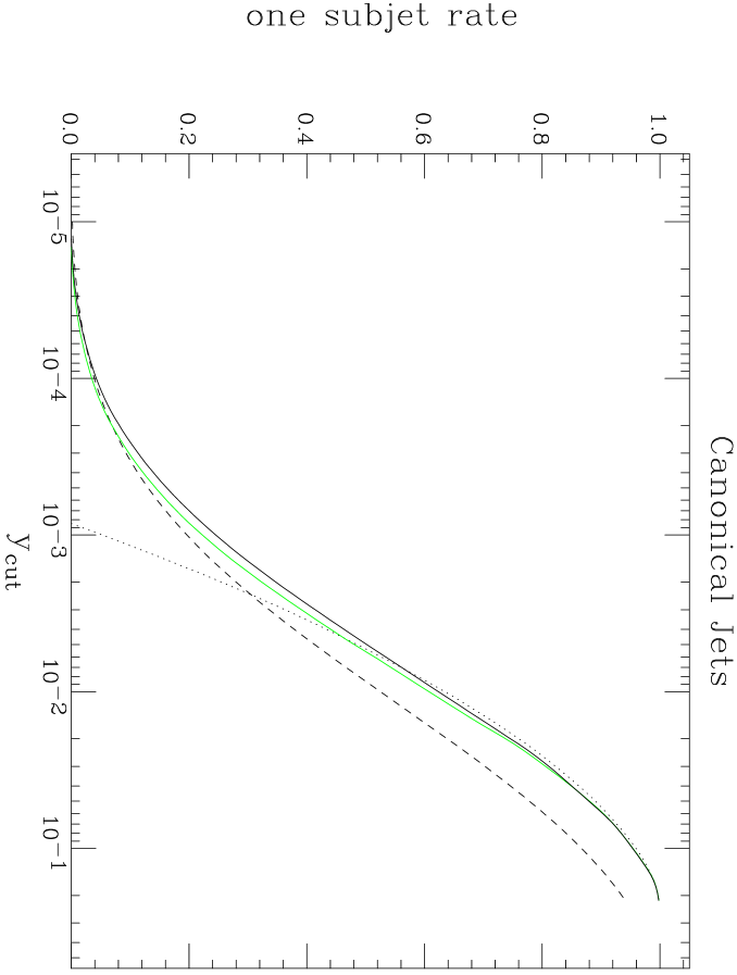
Figure 5: One subjet rate: comparison of leading order (dotted), LLA (dashed), matched NLLA (solid) and matched NLLA with threshold modifications (green).

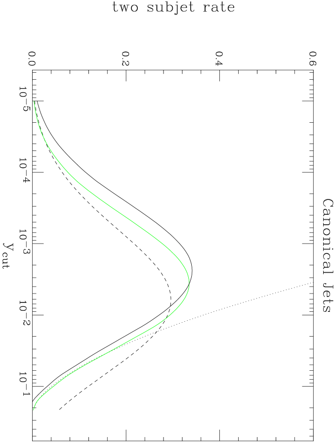
Figure 6: Two subjet rate: comparison of leading order (dotted), LLA (dashed), matched NLLA (solid) and matched NLLA with threshold modifications (green).

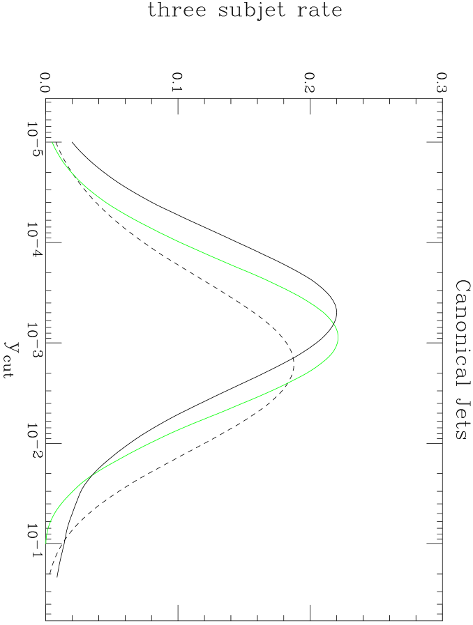
Figure 7: Three subjet rate: comparison of LLA (dashed), matched NLLA (solid) and matched NLLA with threshold modifications (green).

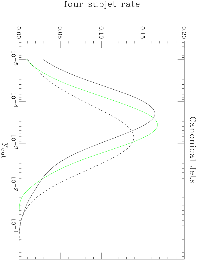
Figure 8: Four subjet rate: comparison of LLA (dashed), matched NLLA (solid) and matched NLLA with threshold modifications (green).

Figures 6–8 show the individual subjet rates in canonical jets for up to and including four subjets. Comparison is made between the leading order prediction, the prediction to leading logarithmic accuracy (LLA) and the fully matched next-to-leading logarithmic accuracy prediction (NLLA) with and without the improved treatment of the threshold region discussed in Sect. 2.2. Firstly, we see that the fixed order results have only a small region of reliability, rapidly becoming unphysical for $y_{\mathrm{cut}}<10^{-2}$. The LLA result is physically behaved, but the higher subjet rates grow much too quickly away from threshold. The matched NLLA results on the other hand should be reliable for all $y_{\mathrm{cut}}$. They approximate the fixed-order results for $P_{1}$ and $P_{2}$ for large $y_{\mathrm{cut}}$ and remain well-behaved for small $y_{\mathrm{cut}}$. We see that the modified threshold treatment makes very little difference for $P_{1}$, slightly more for $P_{2}$ and more still for the higher subjet rates. This is an indication of the relative importance of neglected next-to-next-to-leading logarithmic effects and hence of the accuracy of the whole calculation. This difference would be reduced significantly by matching to the relevant $n$-parton tree-level matrix elements, probably to a similar level to $P_{2}$, but to reduce the dependence further would require working to at least NNLLA. For all subsequent figures we use the threshold-improved results.

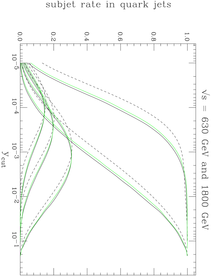
Figure 9: $y_{\mathrm{cut}}$ dependence of subjet rates in quark jets at 630 GeV (green) and 1800 GeV (black) and from final-state logarithms only (dashed). Also shown is the sum of all the rates.

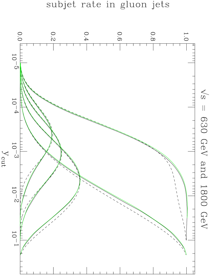
Figure 10: $y_{\mathrm{cut}}$ dependence of subjet rates in gluon jets at 630 GeV (green) and 1800 GeV (black) and from final-state logarithms only (dashed). Also shown is the sum of all the rates.

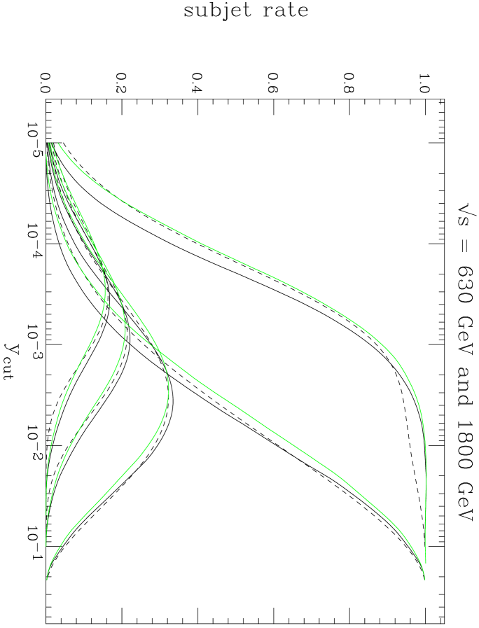
Figure 11: $y_{\mathrm{cut}}$ dependence of subjet rates in all jets at 630 GeV (green) and 1800 GeV (black) and from final-state logarithms only (dashed). Also shown is the sum of all the rates.

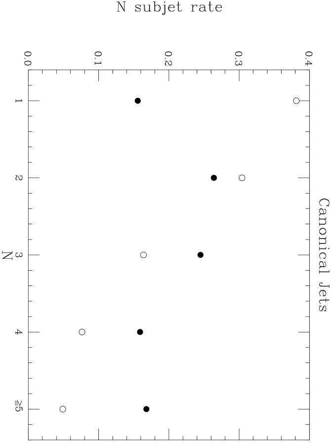
Figure 12: Rates for $N$ subjets at $y_{\mathrm{cut}}~{}=~{}10^{-3}$ in quark (open circles) and gluon (solid circles) jets. The points in the $N=5$ bin are for $N\geq 5$ subjets.

In Figure 10 we show the $y_{\mathrm{cut}}$ dependence of the individual subjet rates in quark jets at the two different collider energies of 630 GeV and 1800 GeV. Figure 10 is a similar plot but for gluon jets and Figure 12 is for all jets. Note the very weak dependence of the rates in quark and gluon jets on the centre-of-mass energy. This result supports the recent DØ analysis where it is assumed that jet observables do not depend upon centre-of-mass energy [9]. One might be tempted to assume, seeing this result and the later ones, that because the properties of quark and gluon jets depend so little on how they were produced they are dominated by final state effects. Comparison with the final-state-only curves in Figures 10 and 10 shows that this is not the case. A significant fraction of the resolved subjets come from non-final-state radiation but are nevertheless still universal to a very good approximation. The all-jets results do vary with centre-of-mass energy, because the quark-to-gluon mix is varying

As discussed at the end of Section 2.4, the effect of initial state radiation cannot be inferred simply from the difference between the dashed and solid lines in Figures 10 and 10. The difference represents the full effect of the $R_{2}-\Delta_{2}$ term in (57), after applying the threshold corrections. This contribution is made up of a logarithmic piece and an order $\alpha_{s}$ piece (see (58)). The logarithmic piece can be termed initial state radiation whilst the latter cannot.

Figure 12 shows the individual subjet rates at fixed $y_{\mathrm{cut}}=10^{-3}$ for canonical quark and gluon jets. The point at $N=5$ is the inferred rate for 5 or more subjets. It has been computed using $P_{n\geq 5}^{a}=1-\sum_{i=1}^{4}P_{i}^{a},$ with the first four subjet rates all shifted to have thresholds at $Y_{5}$, so that $P_{n\geq 5}^{a}$ is sensibly-behaved there.

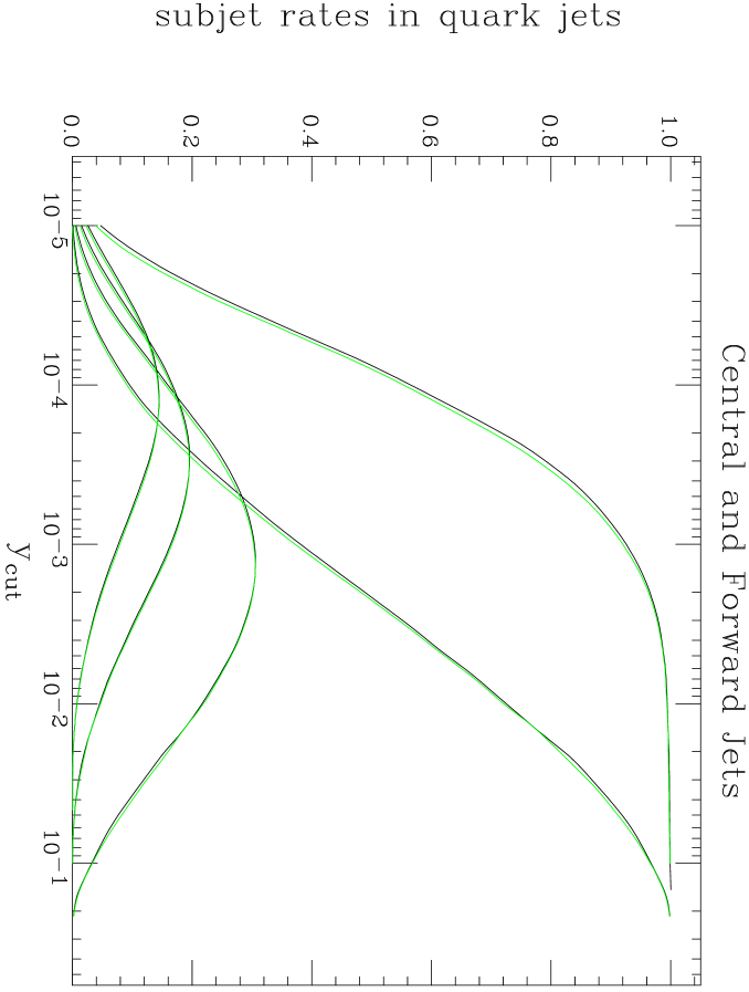
Figure 13: Comparison of subjet rates for $\eta=0$ (black) and $\eta=2$ (green) quark jets.

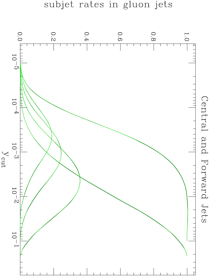
Figure 14: Comparison of subjet rates for $\eta=0$ (black) and $\eta=2$ (green) gluon jets.

We turn now to the rapidity-dependence. Figures 14 and 14 show the $y_{\mathrm{cut}}$ dependence of central ($\eta=0$) and forward ($\eta=2$) jets at $p_{t}=60$ GeV and $\surd s=1800$ GeV. Again they are almost indistinguishable, while the rates for all subjets, Figure 16, do vary owing to the differing mix of quark and gluon jets.

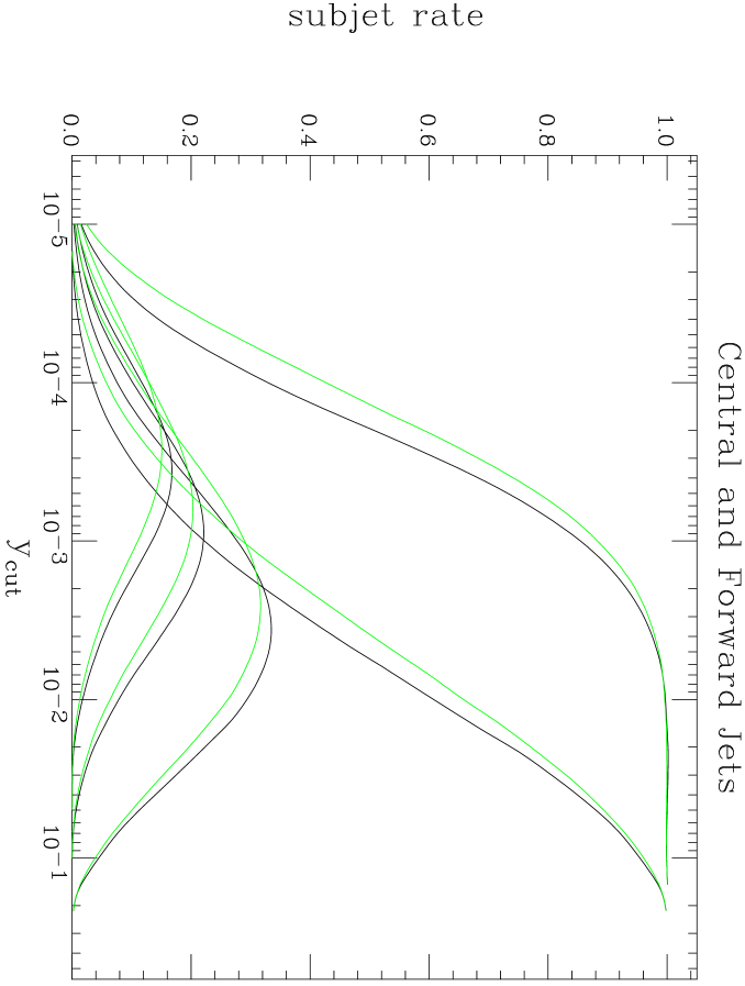
Figure 15: Comparison of subjet rates for $\eta=0$ (black) and $\eta=2$ (green) jets.

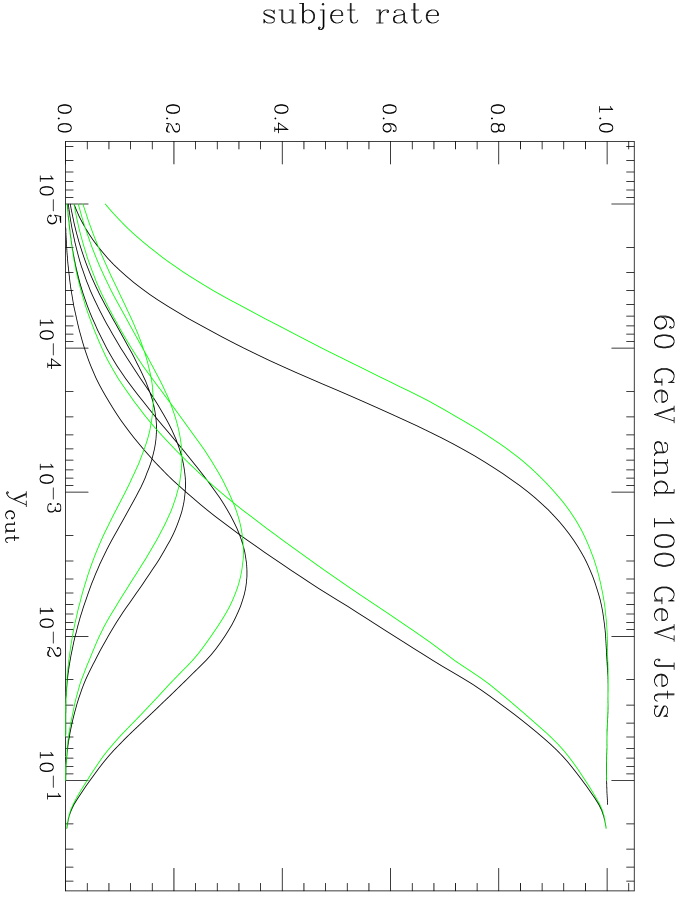
Figure 16: Comparison of subjet rates for jets of $p_{t}=60$ GeV (black) and $p_{t}~{}=~{}100$ GeV (green).

Figure 16 shows the $y_{\mathrm{cut}}$ dependence of $p_{t}=60$ GeV and $p_{t}=100$ GeV jets at $\eta=0$ and $\surd s=1800$ GeV. This time the individual subjet rates for quark (Figure 18) and gluon (Figure 18) jets do depend upon the jet $p_{t}$, because the initial $\alpha_{s}$ value is different.

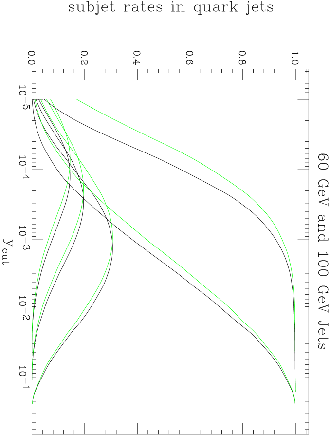
Figure 17: Comparison of subjet rates for quark jets of $p_{t}=60$ GeV (black) and $p_{t}~{}=~{}100$ GeV (green).

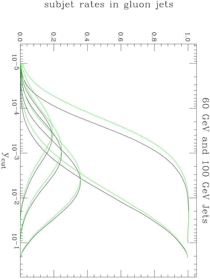
Figure 18: Comparison of subjet rates for gluon jets of $p_{t}=60$ GeV (black) and $p_{t}~{}=~{}100$ GeV (green).

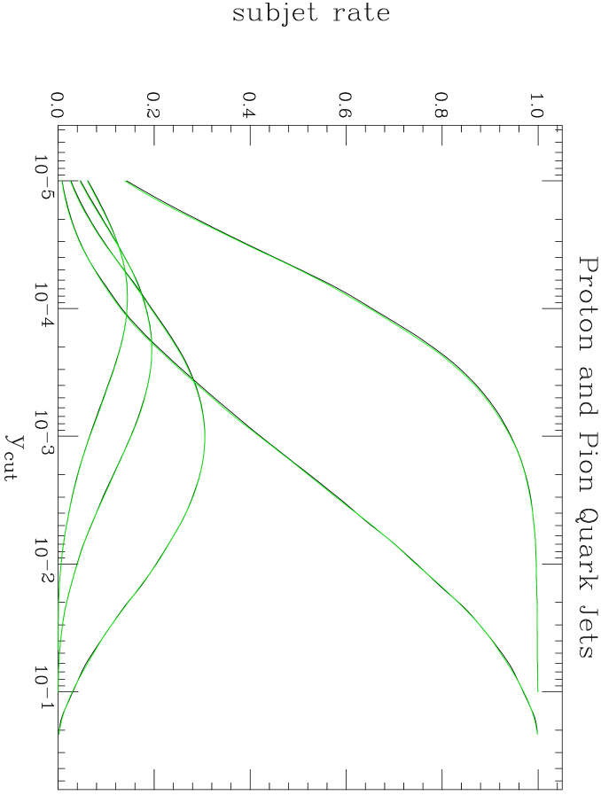
Figure 19: Comparison of subjet rates for quark jets in $p\bar{p}$ collisions (black) and in $\pi^{0}\pi^{0}$ collisions (green).

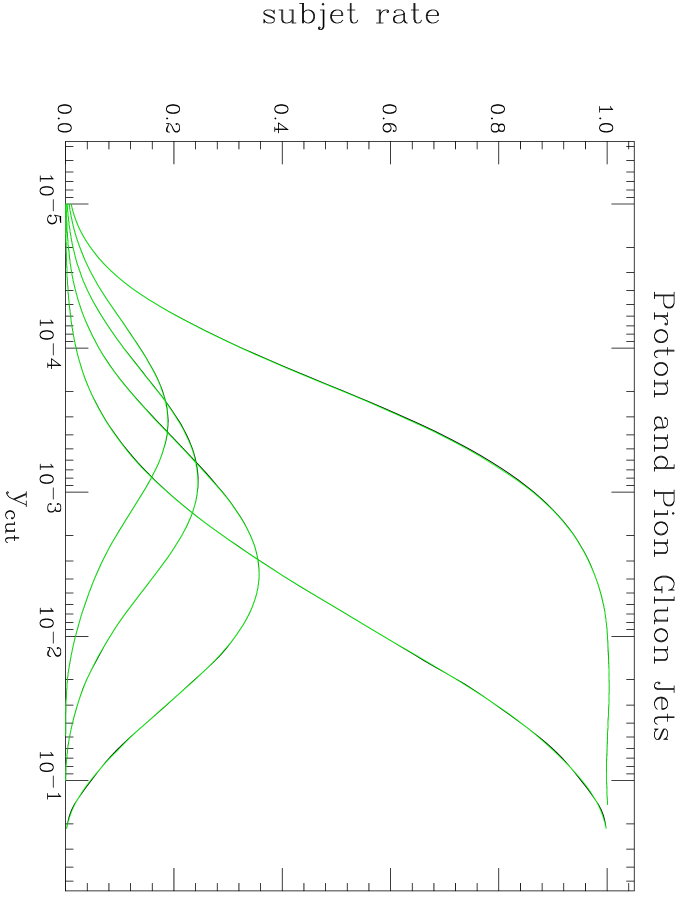
Figure 20: Comparison of subjet rates for gluon jets in $p\bar{p}$ collisions (black) and in $\pi^{0}\pi^{0}$ collisions (green).

Finally, we show in Figures 20 and 20 that not only are the quark and gluon jet properties independent of the collision energy, they are even independent of the collision type, by comparing canonical $p\bar{p}$ jets with those from $\pi^{0}\pi^{0}$ scattering at the same energy. To eliminate spurious differences due to different $\alpha_{s}$ values in the different parton distribution functions, we choose, for these plots only, the GRV sets [17, 18], which use the same $\Lambda$ value for both particle types.

This independence of the properties of a given flavoured jet from the way it was produced is a highly non-trivial result. One would normally expect that the colour coherence of radiation from different emitters in an event would make the soft radiation dependent on the full details of the hard scattering. As mentioned at the end of Section 2.4, the amount of soft initial-state radiation into the jet is in fact largely independent of the scattering kinematics in the fully-inclusive case in which the recoiling jet is integrated out. However, putting requirements on additional jets breaks this inclusivity and the colour coherence changes the properties of the registered jet in response to the kinematics of the other jet.

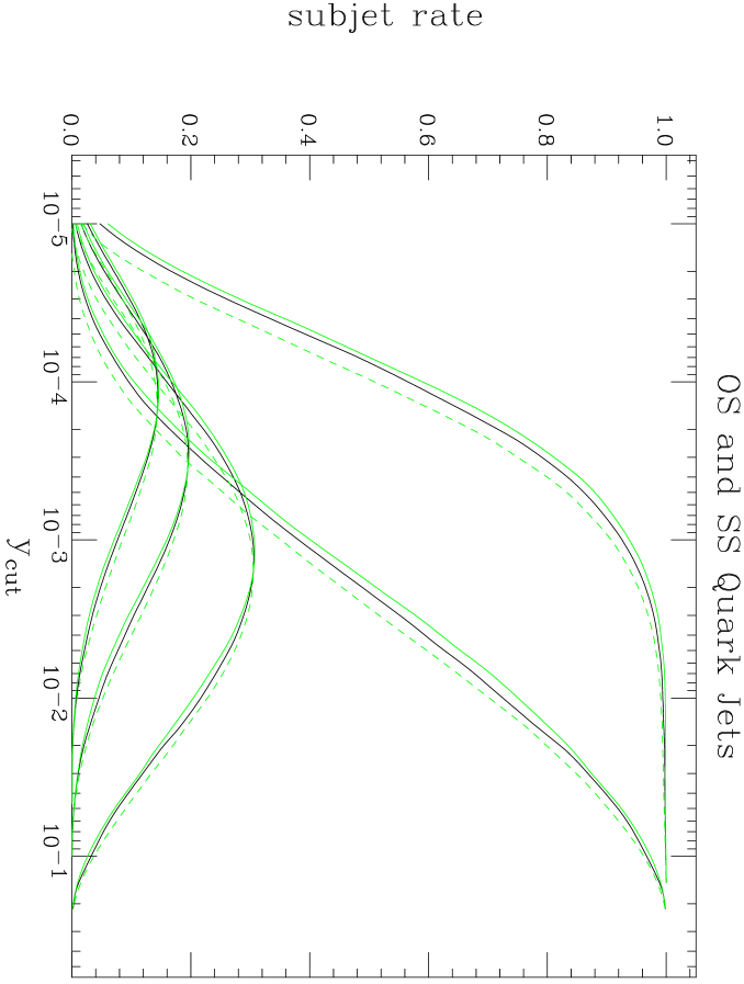
Figure 21: Comparison of subjet rates for quark jets at $\eta=2$ with the other jet in the event allowed to be at any rapidity (black), required to be at $|\eta|=2$ on the same side (solid green) or opposite side (dashed green) of the event.

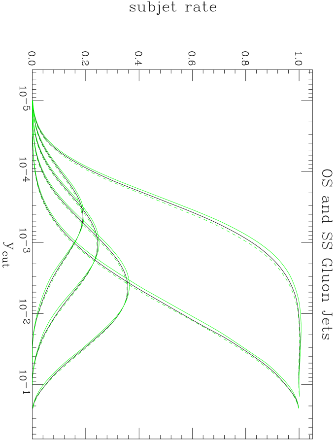
Figure 22: Comparison of subjet rates for gluon jets at $\eta=2$ with the other jet in the event allowed to be at any rapidity (black), required to be at $|\eta|=2$ on the same side (solid green) or opposite side (dashed green) of the event.

This is demonstrated in Figures 22 and 22, where we show the quark and gluon subjet rates for jets at fixed rapidity in the forward region, $\eta=+2$, with the recoiling jet either unconstrained, or required to be at $\eta=+2$ ‘same side’ or $\eta=-2$ ‘opposite side’. The ‘same side/opposite side’ ratio was once thought to be a good way to separate quark and gluon jet properties since, for fixed jet kinematics, the quark-to-gluon mix is very different in the two samples. Figures 22 and 22 show that this is not the case, as the selection itself considerably biases the jet properties. Clearly the method of [9], which uses the centre-of-mass energy-dependence with fixed jet $E_{T}$ is superior.

Although we have not performed a calculation for photoproduction ($\gamma p$ collisions), which has a slightly different structure owing to the direct photon contribution, we expect that the properties of inclusively-defined jets there would be similar to those in hadron collisions, which we have calculated. However, because of the colour coherence effect just mentioned, this statement is unlikely to be true once cuts are made on the other jets in the event. In particular, it is common to try to separate experimentally the direct and resolved photon events by imposing cuts on $x_{\gamma}$, the fraction of the photon’s momentum that is reconstructed in the hardest two jets in the event. It seems likely that this cut will bias the jet properties sufficiently that our calculation cannot be used for a quantitative analysis.

4 Conclusion

We have calculated the subjet rates in hadron collisions to next-to-leading accuracy in logarithms of $y_{\mathrm{cut}}$ to all orders in $\alpha_{s}$, matched with the exact $\mathcal{O}(\alpha_{s})$ result at large $y_{\mathrm{cut}}$. To this accuracy the contribution from initial-state radiation is essential. Nevertheless, it is still possible to separate quark and gluon jets, and we find that their properties are almost completely independent of their production mechanism, depending only on their $p_{t}$, provided that they are defined fully inclusively. As soon as additional cuts are placed on the event, the jet properties become dependent on the details of the hard scattering.

Judging by comparisons of our results with and without threshold matching, which formally differ only by uncalculated next-to-next-to-leading logarithmic terms, we conclude that these terms are rather large, especially for the higher subjet rates. While this situation could certainly be improved by matching the $n$-subjet rate to the tree-level $n\!+\!1$-parton matrix element, further improvement will be extremely difficult. It is likely that, as in $e^{+}e^{-}$ annihilation, $P_{1}$ will remain the best-calculated subjet rate.

References

- [1] G.C. Blazey and B.L. Flaugher, hep-ex/9903058, submitted to Ann. Rev. Nucl. Part. Sci.
- [2] S. Catani, Yu.L. Dokshitzer, F. Fiorani and B.R. Webber, Nucl. Phys. B377 (1992) 445.
-
[3]
S. Catani, Yu.L. Dokshitzer, F. Fiorani and B.R. Webber,
Nucl. Phys. B383 (1992) 419;
G. Gustafson and M. Olsson, Nucl. Phys. B406 (1993) 293;
R. Akers et al. [OPAL Collaboration], Z. Phys. C63 (1994) 363;
D. Buskulic et al. [ALEPH Collaboration], Phys. Lett. B346 (1995) 389;
M. Schmelling, Phys. Scripta 51 (1995) 683;
M.H. Seymour, Phys. Lett. B378 (1996) 279;
S. Lupia and W. Ochs, Phys. Lett. B418 (1998) 214;
D.J. Miller and M.H. Seymour, Phys. Lett. B435 (1998) 199. - [4] Yu.L. Dokshitzer and M. Olsson, Nucl. Phys. B396 (1993) 137.
- [5] S.D. Ellis and D.E. Soper, Phys. Rev. D48 (1993) 3160.
- [6] S. Catani, Yu.L. Dokshitzer, M.H. Seymour and B.R. Webber, Nucl. Phys. B406 (1993) 187.
- [7] M.H. Seymour, Nucl. Phys. B421 (1994) 545.
- [8] S. Catani, Yu.L. Dokshitzer and B.R. Webber, Phys. Lett. B285 (1992) 291.
-
[9]
R. Snihur, ‘Subjet Multiplicity in Quark & Gluon Jets at
DØ’, presented at the DIS99 Workshop, Zeuthen, Germany (1999);
B. Abbott et al. [DØ Collaboration], hep-ex/9907059. - [10] Yu.L. Dokshitzer, V.A. Khoze, A.H. Mueller and S.I. Troyan, “Basics of Perturbative QCD”, Editions Frontières (1991).
- [11] R.K. Ellis, W.J. Stirling and B.R. Webber, “QCD and Collider Physics”, Cambridge University Press (1996).
-
[12]
F.A. Berends, W.T. Giele and H. Kuijf,
Nucl. Phys. B333 (1990) 120;
F.A. Berends and H. Kuijf, Nucl. Phys. B353 (1991) 59. - [13] ZEUS Collaboration, ‘Measurements of Jet Substructure in Photoproduction at HERA’, submitted to EPS99, Tampere, Finland (1999).
- [14] S. Catani, L. Trentadue, G. Turnock and B.R. Webber, Nucl. Phys. B407 (1993) 3.
- [15] H.L. Lai et al. [CTEQ Collaboration], Phys. Rev. D55 (1997) 1280.
- [16] H. Plothow-Besch, Comput. Phys. Commun. 75 (1993) 396.
- [17] M. Glück, E. Reya and A. Vogt, Z. Phys. C67 (1995) 433.
- [18] M. Glück, E. Reya and A. Vogt, Z. Phys. C53 (1992) 651.