DESY 99-037
August 1999
hep-ph/9908289

PREDICTIONS OF ZFITTER v.6 FOR
FERMION-PAIR PRODUCTION WITH ACOLLINEARITY CUT

ZFITTER is a Fortran package for the description of fermion-pair production in $e^{+}e^{-}$-annihilation. We report on results of a rederivation of the complete set of analytical $O(\alpha)$ formulae for the treatment of photonic corrections to the total cross-section and the integrated forward-backward asymmetry with combined cuts on acollinearity angle, acceptance angle, and minimal energy of the fermions. Numerically, the following changes result in ZFITTER v. 6.11 compared to ZFITTER v. 5.20/21: (i) at the $Z$ resonance – numerical changes are negligible; (ii) at LEP 1 energies off-resonance – corrections amount to at most few per mil; (iii) at LEP 2 energies – corrections amount to one per cent or less. Thus, the predictions for LEP/SLC data remain unchanged within the actual errors.

1 Introduction

The Fortran package ZFITTER [?,?,?,?,?,?] is regularly used for the analysis of LEP data since 1989 for the reaction:

$$e^{+}(k_{2})+e^{-}(k_{1})\to{\bar{f}}(p_{2})+f(p_{1})+(n\gamma)(p).$$ (1)

Since the systematic description of ZFITTER  v.4.5 (19 April 1992) [?] a series of improved versions has been released and a nearly complete collection of them may be found in the world wide web [?,?]. Most important updates of recent years are related to the treatment of higher-order corrections. In 1995, this was documented systematically in [?]. Later improvements are described in [?]. The ZFITTER versions 5.20/21 [?] were quite recently followed by versions v.6.nm, beginning with v.6.04/06 [?].

Traditionally we aimed at an accuracy of ZFITTER at LEP 1 energies of the order of 0.5 %. The successful running of LEP 1 together with the precise knowledge of the beam energy however makes an even higher precision necessary [?]: We expect for the final measurements relative errors for total cross-sections and absolute errors for asymmetries of up to 0.15% at the $Z$ peak and of up to 0.5% at $\sqrt{s}=M_{Z}~{}\pm$ several GeV; aiming from the theoretical side ideally at a tenth of these values for the errors of single corrections, we estimate limits of 0.015% and 0.05%, respectively . Similar claims may be found in [?].

First applications of ZFITTER at energies above the $Z$ resonance have become relevant since data from LEP 1.5 and LEP 2 are being analysed. There is also rising interest in applications for the study of the physics potential of a Linear Collider operating at $\sqrt{s}\geq 500$ GeV [?]. At the higher energies, again one generally expects final experimental accuracies of up to 0.8% [?]. So, one should aim at theoretical accuracies of single corrections of up to 0.1 %. The excellent precision of ZFITTER at the $Z$ peak, however, does not automatically guarantee a sufficient accuracy at higher energies, especially since the hard photonic contributions, including higher-order corrections, are no longer suppressed; see Figure 1 and compare to Figure 2.

In 1992, a comparison of ALIBABA v.1 (1991) [?] and ZFITTER v.4.5 (1992) showed deviations between the predictions of the two programs of several per cent [?]; we show one of the plots of that study in Figure 3. These deviations were observed only above the $Z$ peak and only when an acollinearity cut on the fermions was applied; the agreement was much better without this cut. We repeated the comparison in 1998 with ALIBABA v.2 (1991), TOPAZ0 v.4.3 (1998) [?,?], and ZFITTER v.5.14 (1998). The outcome was basically unchanged compared to 1992 as may be seen in Figure 3 of reference [?].

Figure 1: Cross-sections and forward-backward asymmetries for muon-pair production with different acollinearity cuts.

It is well-known that deviations of up to several per cent may result from different treatments of radiative corrections. Recent studies [?] claim for the case of Bhabha scattering that an accuracy of 0.3% for $O(\alpha)$ corrections and of 1% for the complete corrections has been reached at LEP 2 energies as long as the radiative return to the $Z$ peak is prevented by cuts. Similar conclusions were drawn in [?] for fermion-pair production. The radiative return is prevented if $\sqrt{s^{\prime}}>M_{Z}$, i.e. if $R=s^{\prime}/s>M_{Z}^{2}/s$. Our figures contain predictions with an acollinearity cut of $\theta_{\rm acol}<10^{\circ},25^{\circ}$. This corresponds to an $s^{\prime}$-cut of roughly $R>R_{\theta_{\rm acol}}=0.84,0.64$ and $\sqrt{s}>$ 100 GeV, 114 GeV, respectively (see also Table A.1 in the Appendix). The resulting suppression of the radiative return at these and higher energies can nicely be observed in Figure 1. But even if the radiative return is prevented, the influence of hard photonic corrections will be much larger at higher energies than it is near the $Z$ resonance where hard bremsstrahlung is nearly completely suppressed. Figure 2 demonstrates that different portions of hard photon emission lead to nearly identical cross-sections unless the region is reached where even soft photon emission is touched (lowest lying curve).

In this paper, we report on a recalculation of the photonic corrections with acollinearity cut in the ZFITTER approach. In Section 2, we explain changes of flags, subroutines, kinematics, and numerics of ZFITTER. The basic differences to the simpler $s^{\prime}$-cut are explained in subsection 2.2. Section 3 contains few comparisons with other programs and Section 4 a summary.

Figure 2: Muon-pair production cross-sections at LEP 1 energies with different acollinearity cuts.

Figure 3: Muon-pair production cross-section ratios ALIBABA v.1 (1990) versus ZFITTER v.4.5 (1992). An acollinearity cut was applied with $\theta_{\rm acol}^{\max}=25^{\circ}$.

2 Photonic Corrections with Acollinearity Cuts

Perhaps we should remark here that the photonic $O(\alpha)$ corrections in ZFITTER remained basically untouched since about 1989. For the $s^{\prime}$-cut, ZFITTER relies on duplicated analytical calculations [?,?,?,?], and numerical comparisons showed the reliability of the predictions at LEP energies; see e.g. [?] for LEP 1 and [?] for LEP 2. Concerning the acollinearity cut, the situation is different. The corresponding part of ZFITTER [?] was never checked independently, and is not documented. So, we started a complete revision of the $O(\alpha)$ contributions with acollinearity cut. First results were published in [?] where we reported that some deviations from ZFITTER were found for initial-state radiation. We also reported that these deviations could not explain the differences observed when comparing with ALIBABA, while the treatment of higher order corrections evidently was of much higher influence in this respect. Slightly later it was observed in [?] that the perfect agreement of many predictions of ZFITTER v.5.20 and TOPAZ0 v.4.3 at LEP 1 energies of about typically 0.01% could not be reproduced when an acollinearity cut was applied and the initial-final state interference was taken into account. This second puzzle could be resolved by our recalculation; see section 2.4.

By now we have a complete collection of the analytical formulae for the $O(\alpha)$ corrections. The corresponding Fortran package is acol.f. We merged package acol.f with photonic corrections for the integrated total cross-section and the integrated forward-backward asymmetry (with and without acceptance cut) into ZFITTER v.5.21, thus creating ZFITTER v.6.04/06 [?] onwards. The angular distribution will be available in v.6.2 onwards. The remarkably compact expressions for the case that no angular acceptance cut is applied are published [?]. A complete collection of the analytical expressions is in preparation [?].

2.1 Flags and subroutines in ZFITTER

In ZFITTER the calculation of cross sections and asymmetries is dealt with by subroutine ZCUT which either calls subroutines SCUT (angular acceptance cut applied) or SFAST (shorter formulae; no angular acceptance cut). In the latest releases, ZFITTER v.5.20 up to ZFITTER v.6.11, the following flag settings in subroutine ZUCUTS are of relevance here:

• ICUT = –1: cut on the invariant mass of the fermion pair, $s^{\prime}$

• ICUT = 0: cuts on acollinearity and minimal energy of the fermions and on the acceptance angle of one fermion

• ICUT = 1: cuts on $s^{\prime}$ and on the acceptance angle $\vartheta$ of one fermion

Since ZFITTER v.6.04, we introduced two new values of this flag:

• ICUT = 2: new coding of case corresponding to ICUT = 0, but without acceptance cut [?];

• ICUT = 3: new coding of case corresponding to ICUT = 0 [?].

In order to maintain compatibility with earlier releases, the branch ICUT=0 is retained; it calculates with the old coding of the final-state corrections (flag IFUNFIN = 0), while all other branches use the newly corrected final-state contributions (flag IFUNFIN = 1).

All the corrections related to the acollinearity cut are called from essentially only six subroutines/functions of ZFITTER; see Figure 4. The subroutines SHARD and AHARD, or respectively FCROS and FASYM, call the initial-state and initial-final state interference corrections, while FUNFIN calculates final-state corrections (for the case of common exponentiation of initial- and final-state soft photon corrections).

For a detailed description of the Fortran package ZFITTER we refer to [?].

Figure 4: Logical structure of subroutine ZCUT.

2.2 Photonic corrections with acollinearity cut: Kinematics

The phase-space parameterisation

The phase-space parameterisation derived in [?] is used. A three-fold analytical integration of the squared matrix elements had to be performed. The last integration, that over $R=s^{\prime}/s$, is then performed numerically. The Dalitz plot given in Figure 5 may help to understand the relation between a kinematically simple $s^{\prime}$-cut and a more involved acollinearity cut. The variable shown besides $R$ is $x$, the invariant mass of (${\bar{f}}+\gamma$) in the cms. As Figure 5 shows, we have to determine the cross-sections in three phase-space regions with different boundary values of $x$ at given $R$:

$$\frac{d\sigma}{d\cos\vartheta}=\left[\int_{\mathrm{I}}+\int_{\mathrm{II}}-\int_{\mathrm{III}}\right]~{}dR~{}dx\frac{d\sigma}{dRdxd\cos\vartheta}.$$ (2)

Region I corresponds to the simple $s^{\prime}$-cut.

The integration over $R$ extends from $R_{min}$ to 1,

$$R_{min} = R_{E}\left(1-\frac{\sin^{2}(\theta_{\rm acol}^{\max}/2)}{1-R_{E}\cos^{2}(\theta_{\rm acol}^{\max}/2)}\right).$$ (3)

The soft-photon corner of the phase space is at $R=1$. Thus, the additional contributions related to the acollinearity cut are exclusively due to hard photons. The boundaries for the integration over $x$ are, for a given value of $R$:

$$x_{max,min} = \frac{1}{2}(1-R)~{}(1\pm A),$$ (4)

where the parameter $A=A(R)$ depends in every region on only one of the cuts applied:

$$A_{\mathrm{I}} = \sqrt{1-\frac{R_{m}}{R}}\approx 1,$$ (5)

$$A_{\mathrm{II}} = \frac{1+R-2R_{E}}{1-R},$$ (6)

$$A_{\mathrm{III}} = \sqrt{1-\frac{R(1-R_{\theta_{\rm acol}})^{2}}{R_{\theta_{\rm acol}}(1-R)^{2}}},$$ (7)

with:

$$R_{m} = \frac{4m_{f}^{2}}{s},$$ (8)

$$R_{E} = \frac{2E_{min}}{\sqrt{s}},$$ (9)

$$R_{\theta_{\rm acol}} = \frac{1-\sin(\theta_{\rm acol}^{\max}/2)}{1+\sin(\theta_{\rm acol}^{\max}/2)}.$$ (10)

Here, $m_{f}$ and $E_{min}$ are the final-state fermions’ mass and a cut on their individual energies in the cms.

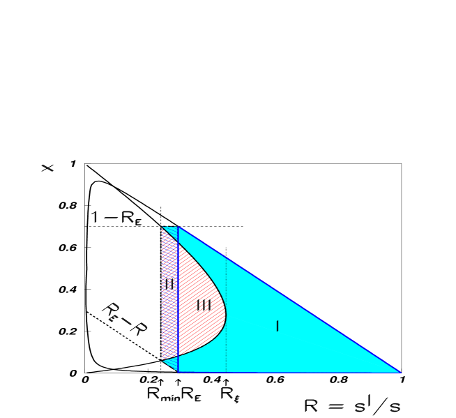
Figure 5: Phase-space with cuts on acollinearity and energy of the fermions.

Mass singularities from initial-state radiation

In the last section we saw that the Dalitz plot in Figure 5 is independent of the scattering angle $\cos\vartheta$. Here we will show that the integrations in regions II and III are nevertheless crucially influenced by $\cos\vartheta$.

The squared matrix elements contain, from initial-state radiation, the electron (positron) propagator, and these terms are proportional to first and second powers of

$$\frac{1}{Z_{1(2)}} = -\frac{1}{(k_{1(2)}-p)^{2}-m_{e}^{2}}=\frac{1}{2k_{1(2)}p}$$ (11)

$$= \frac{1}{A_{1(2)}\pm B\cos\varphi_{\gamma}},$$

with

$$A_{1(2)} = \frac{s}{2}(1-R)(1\pm\beta_{0}\cos\vartheta\cos\theta_{\gamma}),$$ (12)

$$B = \frac{s}{2}(1-R)\beta_{0}\sin\vartheta\sin\theta_{\gamma},$$ (13)

and

$$\beta_{0} = \sqrt{1-4m_{e}^{2}/s},$$ (14)

$$\cos\theta_{\gamma} = \frac{\lambda_{1}-\lambda_{2}-\lambda_{p}}{2\sqrt{\lambda_{2}\lambda_{p}}},$$ (15)

$$\sqrt{\lambda_{1}} = (1-x)s,$$ (16)

$$\sqrt{\lambda_{2}} = (x+R)s,$$ (17)

$$\sqrt{\lambda_{p}} = (1-R)s.$$ (18)

For the calculation of the initial-state corrections we may neglect final-state mass effects.

The first analytical integration is over $\varphi_{\gamma}$, the photon production angle in the ($f+\gamma$) rest system [?]:

$$\frac{d\sigma}{dRdxd\cos\vartheta} = \int_{0}^{2\pi}d\varphi_{\gamma}\frac{d\sigma}{dRdxd\cos\vartheta d\varphi_{\gamma}}.$$ (19)

It is important to take care of the electron mass $m_{e}$, e.g. in the following contribution:

$$\int^{2\pi}_{0}d{\varphi_{\gamma}}\,\frac{1}{Z_{i}(R,\cos\vartheta,x,\varphi_{\gamma})} = \frac{2\pi\sqrt{\lambda_{2}}}{\sqrt{C_{i}}},$$ (20)

$$C_{i} = s^{2}a_{i}x^{2}-2sb_{i}x+c_{i},$$ (21)

$$a_{i} = s^{2}(z_{i}^{2}-R\,\eta_{0}^{2}),$$ (22)

$$b_{i} = s^{3}[R\,z_{i}\,(1-z_{i})-\frac{1}{2}\,R(1-R)\,\eta_{0}^{2}],$$ (23)

$$c_{i} = s^{4}\,R^{2}\,(1-z_{i})^{2},$$ (24)

$$z_{1(2)} = \frac{1\mp\beta_{0}\cos\vartheta}{2}+R\frac{1\pm\beta_{0}\cos\vartheta}{2}$$ (25)

$$\eta_{0}^{2} = 1-\beta_{0}^{2};\quad\beta_{0}^{2}=1-\frac{4m_{e}^{2}}{s}.$$ (26)

Be the next integration that over $x$ with limits (4). Consider e.g. the following integral:

$$I_{i}^{0}(R,\cos\vartheta) = \int\limits_{x_{min}}^{x_{max}}\frac{sdx}{\sqrt{C_{i}}}$$ (27)

$$= \frac{1}{\sqrt{a_{i}}}\left.\ln\left[\sqrt{a_{i}}C_{i}^{\frac{1}{2}}+(sa_{i}x-b_{i})\right]\right|^{x_{max}}_{x_{min}},$$

with

$$C_{i}|_{x_{max,min}} = \frac{1}{4}\,s^{4}(1-R)^{2}\left[(y_{i}\pm Az_{i})^{2}+R\,(1-A^{2})\,\eta_{0}^{2}\right],$$ (28)

$$y_{1(2)} = \frac{1\mp\beta_{0}\cos\vartheta}{2}-R\frac{1\pm\beta_{0}\cos\vartheta}{2},$$ (29)

and

$$(sa_{i}x-b_{i})\Biggr{|}^{x_{max}}_{x_{min}} = (1-R)(y_{i}\pm Az_{i})+O(\eta_{0}^{2}).$$ (30)

We are interested in the limit of vanishing electron mass $m_{e}$ for the subsequent integrations. In this limit there will occur zeros in arguments of logarithms like that in (27) at four locations defined by the conditions:

$$(y_{i}\pm Az_{i})=0,~{}~{}~{}~{}~{}i=1,2.$$ (31)

These zeros appear as functions of $\cos\vartheta$ with parameters $R$ and $A=A(R)$ at certain values $\cos\vartheta=c_{i}^{\pm}$ ($i=1,2$):

$$c_{2}^{+} = \frac{1-R+A(R)(1+R)}{1+R+A(R)(1-R)}\geq 0,$$ (32)

$$c_{2}^{-} = \frac{1-R-A(R)(1+R)}{1+R-A(R)(1-R)},$$ (33)

$$c_{1}^{-} = -c_{2}^{-},$$ (34)

$$c_{1}^{+} = -c_{2}^{+}\leq 0.$$ (35)

The relations $c_{2}^{+}\geq c_{2}^{-}$ and $c_{1}^{+}\leq c_{1}^{-}$ are also fulfilled. In the course of the integrations different analytical expressions have to be used in different kinematical regions when neglecting $m_{e}$ wherever possible. As a result of all that we have to cut the remaining phase space for $\cos\vartheta$ (at fixed $R$ and for given $i$) into three different regions. It is region I (with the $s^{\prime}$-cut) where the conditions (32) to (35) become trivial:

$$c_{2}^{+}(I)=-c_{2}^{-}(I)=c_{1}^{-}(I)=-c_{1}^{+}(I)=1.$$ (36)

There, only one case has to be considered ($-1\leq\cos\vartheta\leq 1$). In regions II and III, the differential cross-section ${d{\sigma}}/({dRd{\cos\vartheta}})$ is a double-sum over $i=1,2$ and has different analytical expressions for each combination of the kinematical ranges defined by (32) to (35).

The final result for e.g. $I^{0}_{i}$ after integration over $x$ setting $m_{e}=0$ becomes ($i=1,2$):
(i) for $|\cos\vartheta|<|c^{-}_{i}|$ with $y_{i}\pm Az_{i}>0$ (case ”$i++$”):

$$I_{i}^{0}=\frac{1}{sz_{i}}\ln\left(\frac{y_{i}+Az_{i}}{y_{i}-Az_{i}}\right)$$ (37)

(ii) for $|c^{-}_{i}|<|\cos\vartheta|<|c^{+}_{i}|$ with $y_{i}+Az_{i}>0$ and $y_{i}-Az_{i}<0$ (case ”$i+-$”):

$$I_{i}^{0}=\frac{1}{sz_{i}}\left\{\ln\left[\frac{z_{i}^{2}(y_{i}+Az_{i})(Az_{i}-y_{i})}{R^{2}(1-\beta_{0}^{2}\cos^{2}\vartheta)}\right]+\ln\left(\frac{s}{m_{e}^{2}}\right)\right\},$$ (38)

(iii) for $|\cos\vartheta|>|c^{+}_{i}|$ with $y_{i}\pm Az_{i}<0$ (case ”$i--$”):

$$I_{i}^{0}=-\frac{1}{sz_{i}}\ln\left(\frac{y_{i}+Az_{i}}{y_{i}-Az_{i}}\right).$$ (39)

One may show that the resulting number of cases for the angular distribution, depending on the value of $\cos\vartheta$ with respect to $c^{\pm}_{i}$ and on $R$, is at most four in regions II and III. These are for $\cos\vartheta\geq 0$ with the abbreviations given in eq. (37) to (39):
a. ”$1++$” combined with ”$2++$”;
b. ”$1+-$” combined with ”$2+-$”;
c. ”$1++$” combined with ”$2+-$”;
d. ”$1--$” combined with ”$2++$”.
For $\cos\vartheta<0$ cases c. and d. are exchanged by:
a. ”$1++$” combined with ”$2++$”;
b. ”$1+-$” combined with ”$2+-$”;
c.’ ”$1+-$” combined with ”$2++$”;
d.’ ”$1++$” combined with ”$2--$”.
For region I (the $s^{\prime}$-cut) only case b. is possible. This simplification follows from $A=1$; see above.

When integrating over $\cos\vartheta$ within acceptance cut boundaries $\pm c$, the distinction of different regions in phase space has to be repeated where the cut-off $c$ now plays the role of $\cos\vartheta$. Depending on the relative position of $c$ with respect to the values $c_{i}^{\pm}$ we have to integrate over different expressions of the angular distribution (indicated above by the distinction of cases a. to d., or a. to d.’ respectively) in the remaining $\cos\vartheta$-$R$ phase space. One finally gets at most four different analytical expressions for $\sigma_{T}^{hard}(R;c,A)$ and six for $\sigma_{FB}^{hard}(R;c,A)$ in different regions of phase space. This is because of symmetric cancellations when integrating over $\cos\vartheta$: $\sigma_{T}^{hard}=\int^{c}_{-c}{d\cos\vartheta}\,{d\sigma^{hard}}/{d\cos\vartheta}$, while $\sigma_{FB}^{hard}=\left(\int^{c}_{0}-\int^{0}_{-c}\right){d\cos\vartheta}\,{d\sigma^{hard}}/{d\cos\vartheta}$. It is the additional occurance of $c=0$ in the definition of $\sigma_{FB}^{hard}$ that leads to more cases.

If no acceptance cut is applied, $c=1$, only one case remains for $\sigma_{T}^{hard}=\sigma(1)-\sigma(-1)$ in regions II and III – because then $-1<c^{\pm}_{i}<1$ (see cases d. and d’ above) – while for $\sigma_{FB}^{hard}$ two of them are left because the additional integrated contributions from $\cos\vartheta=0$ depend on whether $c^{-}_{2}>0$ or not ($c^{-}_{2}=-c^{-}_{1}$): $\sigma_{FB}^{hard}=\sigma(1)-2\sigma(0)+\sigma(-1)$. The conditions (33) and (34) are fulfilled for $\cos\vartheta=0$ with

$$A_{0} = \frac{1-R}{1+R},$$ (40)

so that, depending on $A(R)$, one or the other analytical expression has to be used. This was practised in [?].

One can check that the integrated results $\sigma_{T,FB}^{hard}$ are continuous when $c\rightarrow c_{i}^{\pm}$ while $d\sigma^{hard}/d\cos\vartheta$ can be regularised at $\cos\vartheta=c_{i}^{\pm}$ taking the exact logarithmic results in $m_{e}$ for the integrals.

One can also reassure oneself that the contributions proportional to the Born cross-section $\sigma^{0}$ and Born asymmetry $A_{FB}$ are (anti)symmetric respectively as it should be for the one loop corrected initial-state results. We will come to this in the next section.

The phase-space splitting discussed above has also an influence on the initial-final state interference corrections since there the initial-state propagators with $Z_{1,2}^{-1}$ appear linearly. They will not contribute in the final-state contributions so that the phase-space splitting is not necessary there.

2.3 Initial-state radiation

We systematically compared numerical predictions of ZFITTER v.5.20 and ZFITTER v.6.11 with default flag settings. Version 5.20 was used as released, while version 6.11 was prepared such that the changes due to the recalculation of initial-state corrections, final-state corrections, their interferences, and the net effect could be isolated. We begin with a study of the changes related to initial-state radiation.

For $\sigma_{T}$, the changes are at most one unit in the fifth digit at LEP 1 energies and thus considered to be completely negligible. In Table 1 we show the corresponding shifts of predictions for $A_{FB}$ for two acollinearity cuts, $\theta_{\rm acol}<10^{\circ},25^{\circ}$, and three different acceptance cuts, $\vartheta_{acc}=0^{\circ},20^{\circ},40^{\circ}$. The changes are also less than the theoretical accuracies demanded. We checked that our numbers for ICUT = 0 agree with the ZFITTER predictions shown in Tables 26 and 27 of [?].

In Figure 6 the ratio of $\sigma_{T}$ from ZFITTER v.6.11 and v.5.20 and in Figure 7 the difference of $A_{FB}$ are shown in a wider energy range. While at energies slightly above the $Z$ peak the differences of the predictions show local peaks, at LEP 2 energies and beyond they are negligible for $\sigma_{T}$ and amount to only 0.1% – 0.2% for $A_{FB}$. The peaking structures disappear at energies for which the radiative return is prohibited by the cuts. In dependence on the acollinearity cut, this happens for energies $s>s^{min}$. The $s^{min}$ is calculated in Appendix A.

$A^{\mu}_{{}_{\rm FB}}$ with $\theta_{\rm acol}<10^{\circ}$
$\theta_{\rm acc}$	$M_{{}_{Z}}-3$	$M_{{}_{Z}}-1.8$	$M_{{}_{Z}}$	$M_{{}_{Z}}+1.8$	$M_{{}_{Z}}+3$
$0^{\circ}$	-0.28462	-0.16916	0.00024	0.11482	0.16063
	-0.28453	-0.16911	0.00025	0.11486	0.16071
$20^{\circ}$	-0.27521	-0.16355	0.00032	0.11141	0.15602
	-0.27506	-0.16347	0.00035	0.11148	0.15616
$40^{\circ}$	-0.24230	-0.14398	0.00045	0.09881	0.13868
	-0.24207	-0.14386	0.00050	0.09893	0.13891
$A^{\mu}_{{}_{\rm FB}}$ with $\theta_{\rm acol}<25^{\circ}$
$\theta_{\rm acc}$	$M_{{}_{Z}}-3$	$M_{{}_{Z}}-1.8$	$M_{{}_{Z}}$	$M_{{}_{Z}}+1.8$	$M_{{}_{Z}}+3$
$0^{\circ}$	-0.28651	-0.17051	-0.00043	0.11292	0.15680
	-0.28647	-0.17049	-0.00043	0.11293	0.15682
$20^{\circ}$	-0.27727	-0.16499	-0.00038	0.10942	0.15201
	-0.27722	-0.16497	-0.00037	0.10944	0.15204
$40^{\circ}$	-0.24452	-0.14549	-0.00027	0.09675	0.13449
	-0.24445	-0.14545	-0.00026	0.09678	0.13454

Table 1: Comparison of ZFITTER v.6.11 (first row) with ZFITTER v.5.20 (second row) for the muonic forward-backward asymmetry with angular acceptance cut ($\theta_{\rm acc}=0^{\circ},20^{\circ},40^{\circ}$) and acollinearity cut ($\theta_{\rm acol}<10^{\circ},25^{\circ}$); $M_{{}_{Z}}=91.1867$ (GeV). The initial-final state interference is switched off and only initial-state radiation is corrected.

For the case of initial-state radiation, we were able to trace back the reason of the numerical inaccuracies related to the acollinearity cut of ZFITTER below version 6. It is the result of leaving out a certain class of non-logarithmic, simple terms of order $O(\alpha)$. For $\sigma_{T}$, polynomials proportional to $\cos\vartheta$ (and their integrals) are concerned, and for $\sigma_{FB}$ polynomials of the type $(a+b\cos^{2}\vartheta)$ (and their integrals). At first glance the corresponding contributions seem to vanish for symmetric acceptance cuts. But this is not the case! As we explained in Section 2.2, the cross-section formulae lose the usual simple symmetry/anti-symmetry behaviour under the transformation $\cos\vartheta\leftrightarrow(-\cos\vartheta)$ in regions II and III of the phase space since different analytical expressions may be needed depending on the location of the parameters $c_{i}^{\pm}$ describing the solutions of (31). Then, the symmetry behaviour as a function of $\cos\vartheta$ is ”hidden” since different regions contribute differently to the net result.

Figure 6: Ratios of muon-pair production cross-sections predicted from ZFITTER v.6.11 and v.5.20 without and with acceptance cut and with three different acollinearity cuts: $\theta_{\rm acol}<10^{\circ},25^{\circ},90^{\circ}$; $E_{min}=1$ GeV; programs differ by initial-state radiation.

Figure 7: Differences of muonic forward-backward asymmetries predicted from ZFITTER v.6.11 and v.5.20 without and with acceptance cut and with three different acollinearity cuts: $\theta_{\rm acol}<10^{\circ},25^{\circ},90^{\circ}$; $E_{min}=1$ GeV; programs differ by initial-state radiation.

2.4 Initial-final state interference

The ZFITTER v.5 predictions of photonic corrections from the initial-final state interference also receive modifications due to the recalculation for the versions v.6. The explanation given in Section 2.3 for the case of initial-state radiation is also applicable for a part of the deviations here. The codings for the initial-final state interference also show additional deviations in the hard photonic corrections and the resulting numerical differences are much larger.

$\sigma_{\mu}\,$[nb] with $\theta_{\rm acol}<10^{\circ}$						$\sigma_{\mu}\,$[nb] with $\theta_{\rm acol}<25^{\circ}$
$\theta_{\rm acc}$	$M_{{}_{Z}}-3$	$M_{{}_{Z}}-1.8$	$M_{{}_{Z}}$	$M_{{}_{Z}}+1.8$	$M_{{}_{Z}}+3$	$\theta_{\rm acc}$	$M_{{}_{Z}}-3$	$M_{{}_{Z}}-1.8$	$M_{{}_{Z}}$	$M_{{}_{Z}}+1.8$	$M_{{}_{Z}}+3$
Z6 $0^{\circ}$	0.21928	0.46285	1.44780	0.67721	0.39360	Z6 $0^{\circ}$	0.22328	0.46968	1.46598	0.68688	0.40031
	0.21772	0.46082	1.44776	0.67898	0.39489		0.22228	0.46836	1.46602	0.68816	0.40128
	-7.16	-4.41	-0.03	+2.60	+3.27		-4.51	-2.82	+0.03	+1.86	+2.41
Z5 $0^{\circ}$	0.21928	0.46285	1.44781	0.67722	0.39361	Z5 $0^{\circ}$	0.22328	0.46968	1.46598	0.68688	0.40031
	0.21852	0.46186	1.44782	0.67814	0.39429		0.22281	0.46905	1.46603	0.68754	0.40081
	-3.48	-2.14	+0.01	+1.36	+1.72		-2.11	-1.34	+0.03	+0.96	+1.25
Z6 $20^{\circ}$	0.19987	0.42205	1.32053	0.61756	0.35881	Z6 $20^{\circ}$	0.20357	0.42834	1.33718	0.62647	0.36505
	0.19869	0.42046	1.32018	0.61877	0.35972		0.20281	0.42729	1.33689	0.62731	0.36572
	-5.96	-3.79	-0.27	+1.95	+2.53		-3.74	-2.46	-0.21	+1.35	+1.83
Z5 $20^{\circ}$	0.19987	0.42205	1.32053	0.61756	0.35881	Z5 $20^{\circ}$	0.20357	0.42833	1.33718	0.62647	0.36505
	0.19892	0.42075	1.32021	0.61857	0.35959		0.20321	0.42781	1.33689	0.62684	0.36536
	-4.78	-3.09	-0.24	+1.63	+2.17		-1.77	-1.22	-0.22	+0.59	+0.85
Z6 $40^{\circ}$	0.15032	0.31760	0.99416	0.46475	0.26983	Z6 $40^{\circ}$	0.15318	0.32243	1.00682	0.47164	0.27477
	0.14974	0.31675	0.99349	0.46515	0.27019		0.15280	0.32183	1.00619	0.47188	0.27502
	-3.88	-2.72	-0.67	+0.87	+1.32		-2.48	-1.88	-0.62	+0.51	+0.91
Z5 $40^{\circ}$	0.15032	0.31760	0.99415	0.46474	0.26983	Z5 $40^{\circ}$	0.15318	0.32243	1.00682	0.47164	0.27477
	0.14978	0.31680	0.99350	0.46511	0.27016		0.15287	0.32192	1.00619	0.47180	0.27496
	-3.61	-2.53	-0.65	+0.80	+1.22		-2.03	-1.58	-0.63	+0.34	+0.69

Table 2: Comparison of ZFITTER v.6.11 (first row) with ZFITTER v.5.20 (second row) for muon-pair production cross-sections with angular acceptance cuts ($\theta_{\rm acc}=0^{\circ},20^{\circ},40^{\circ}$) and acollinearity cut ($\theta_{\rm acol}<10^{\circ},25^{\circ}$). First row is without initial-final state interference, second row with, third row the relative effect of that interference in per mil. Final-state treated as in v.5.20.

In Table 2 we show the shifts of predictions for muon-pair production due to the initial-final state interference for two choices of the acollinearity cut. Table 3 shows the corresponding effects for the forward-backward asymmetry. The two tables are the analogues to Tables 37–40 of [?], where TOPAZ0 v.4.3 and ZFITTER v.5.20 were compared. At the $Z$ peak, the predictions for the influence of the initial-final state interference from ZFITTER v.5.20 and ZFITTER v.6.11 deviate from each other only negligibly, with maximal deviations of up to 0.015%. At the wings, the situation is quite different; we observe deviations of up to several per mil for cross-sections and up to a per mil for asymmetries. The deviations between the two codings decrease if the acollinearity cut is weakened.

$A^{\mu}_{{}_{\rm FB}}$ with $\theta_{\rm acol}<10^{\circ}$						$A^{\mu}_{{}_{\rm FB}}$ with $\theta_{\rm acol}<25^{\circ}$
$\theta_{\rm acc}$	$M_{{}_{Z}}-3$	$M_{{}_{Z}}-1.8$	$M_{{}_{Z}}$	$M_{{}_{Z}}+1.8$	$M_{{}_{Z}}+3$	$\theta_{\rm acc}$	$M_{{}_{Z}}-3$	$M_{{}_{Z}}-1.8$	$M_{{}_{Z}}$	$M_{{}_{Z}}+1.8$	$M_{{}_{Z}}+3$
Z6 $0^{\circ}$	-0.28462	-0.16916	0.00024	0.11482	0.16063	Z6 $0^{\circ}$	-0.28651	-0.17051	-0.00043	0.11292	0.15680
	-0.28187	-0.16689	0.00083	0.11379	0.15907		-0.28554	-0.16960	-0.00000	0.11285	0.15669
	+2.75	+2.27	+0.60	-1.03	-1.56		+0.97	+0.91	+0.43	-0.06	-0.11
Z5 $0^{\circ}$	-0.28453	-0.16911	0.00025	0.11486	0.16071	Z5 $0^{\circ}$	-0.28647	-0.17049	-0.00043	0.11293	0.15682
	-0.28282	-0.16783	0.00070	0.11475	0.16059		-0.28555	-0.16975	-0.00005	0.11307	0.15701
	+1.71	+1.28	+0.45	-0.11	-0.12		+0.92	+0.74	+0.48	+0.14	+0.19
Z6 $20^{\circ}$	-0.27521	-0.16355	0.00032	0.11141	0.15602	Z6 $20^{\circ}$	-0.27727	-0.16499	-0.00038	0.10942	0.15201
	-0.27285	-0.16167	0.00080	0.11053	0.15467		-0.27659	-0.16436	-0.00006	0.10943	0.15199
	+2.35	+1.88	+0.47	-0.89	-1.35		+0.68	+0.63	+0.32	+0.00	-0.02
Z5 $20^{\circ}$	-0.27506	-0.16347	0.00035	0.11148	0.15616	Z5 $20^{\circ}$	-0.27722	-0.16497	-0.00037	0.10944	0.15204
	-0.27408	-0.16261	0.00070	0.11133	0.15594		-0.27657	-0.16447	-0.00009	0.10963	0.15229
	+0.98	+0.86	+0.35	-0.15	-0.22		+0.65	+0.50	+0.28	+0.19	+0.25
Z6 $40^{\circ}$	-0.24230	-0.14398	0.00045	0.09881	0.13868	Z6 $40^{\circ}$	-0.24452	-0.14549	-0.00027	0.09675	0.13449
	-0.24063	-0.14277	0.00073	0.09825	0.13780		-0.24423	-0.14527	-0.00010	0.09687	0.13464
	+1.67	+1.22	+0.28	-0.56	-0.88		+0.29	+0.22	+0.17	+0.12	+0.15
Z5 $40^{\circ}$	-0.24207	-0.14386	0.00050	0.09893	0.13891	Z5 $40^{\circ}$	-0.24445	-0.14545	-0.00026	0.09678	0.13454
	-0.24151	-0.14343	0.00069	0.09890	0.13888		-0.24444	-0.14542	-0.00011	0.09700	0.13483
	+0.56	+0.43	+0.19	-0.03	-0.03		+0.01	+0.03	+0.15	+0.22	+0.29

Table 3: Comparison of ZFITTER v.6.11 (first row) with ZFITTER v.5.20 (second row) for the muonic forward-backward asymmetry with angular acceptance cuts ($\theta_{\rm acc}=0^{\circ},20^{\circ},40^{\circ}$) and acollinearity cut ($\theta_{\rm acol}<10^{\circ},25^{\circ}$). First row is without initial-final state interference, second row with, third row the relative effect of that interference in per mil. Final-state treated as in v.5.20.

In Figure 8 the corresponding shifts are shown for $\sigma_{T}$ (relative units) for $\theta_{acc}=0^{\circ},40^{\circ}$, and in Figure 9 with $\theta_{acc}=0^{\circ},40^{\circ}$, for $A_{FB}$ (absolute units) in a wide range of energies. For the cross-sections, the deviations may reach at most up to 1% at LEP 2 energies, while for asymmetries they stay below 0.5% there. Both shifts are more than the precision we aim at for the theoretical predictions.

Figure 8: Ratios of muon-pair production cross-sections predicted from ZFITTER v.6.11 and v.5.20 without and with acceptance cut and with three different acollinearity cuts: $\theta_{\rm acol}<10^{\circ},25^{\circ},90^{\circ}$; $E_{min}=1$ GeV; programs differ by initial-final state interference.

Figure 9: Differences of muonic forward-backward asymmetries predicted from ZFITTER v.6.11 and v.5.20 without and with acceptance cut and with three different acollinearity cuts: $\theta_{\rm acol}<10^{\circ},25^{\circ},90^{\circ}$; $E_{min}=1$ GeV; programs differ by initial-final state interference.

2.5 Final-state corrections

For the case of final-state radiation, common soft-photon exponentiation together with initial-state radiation is foreseen in ZFITTER. For an $s^{\prime}$-cut, ZFITTER follows [?]. As may be seen from [?] (for the angular distributions) or from [?] (for integrated observables), the predictions for common soft-photon exponentiation include one additional integration, namely that over the invariant mass of the final-state fermion pair at a given reduction of $s$ into $s^{\prime}$ after initial-state radiation. This additional integration is called from subroutine FUNFIN and is treated in ZFITTER in a mixed approach. For not too involved integrands, the integration was performed analytically, while the integration of two logarithms is being done numerically using the Lagrange interpolating formula for the integrand (subroutine INTERP and functions FAL1 and FAL2). A lattice of 20 points is used with subroutine INTERP, and defining a more dense lattice gave no improvements. In ZFITTER v.5, we found a wrong sign of the term $D_{2}$ in variable SFIN in subroutine FUNFIN and a wrong definition of the argument of function FAL2. The former contributes to $\sigma_{T}$, the latter to $\sigma_{FB}$. Additionally, we checked the numerical stability related to the numerical integration. We see also no problem related to a neglect of some $\cos\vartheta$ dependent terms for $\sigma_{T}$ in subroutine FUNFIN.

The variables mentioned above are defined in [?].

For LEP 1, the numerical outcome of our minor improvements is shown in Table 4 (for $\theta_{\rm acol}<10^{\circ},25^{\circ}$) for $A_{FB}$ at several different acceptance cuts: $\vartheta_{acc}=0^{\circ},20^{\circ},40^{\circ}$. Again, our numbers for ICUT = 0 agree with those shown in Tables 26 and 27 of [?]. All the changes are though visible, but negligible. For the cross-sections, the differences are completely negligible and not tabulated here.

In Figure 10, the corresponding shifts from ZFITTER v.5.20 to v.6.11 are shown for $\sigma_{T}$ (relative units) and for $A_{FB}$ (absolute units) in a wide energy range for the case without acceptance cut. We see that the deviations are also negligible in the wide energy range, never exceeding 0.01% for the cross-section and 0.1% for the asymmetry. If an acceptance cut is applied, the changes are yet smaller.

$A^{\mu}_{{}_{\rm FB}}$ with $\theta_{\rm acol}<10^{\circ}$
$\theta_{\rm acc}$	$M_{{}_{Z}}-3$	$M_{{}_{Z}}-1.8$	$M_{{}_{Z}}$	$M_{{}_{Z}}+1.8$	$M_{{}_{Z}}+3$
$0^{\circ}$	-0.28487	-0.16932	0.00025	0.11500	0.16091
	-0.28453	-0.16911	0.00025	0.11486	0.16071
$20^{\circ}$	-0.27539	-0.16367	0.00035	0.11162	0.15635
	-0.27506	-0.16347	0.00035	0.11148	0.15616
$40^{\circ}$	-0.24236	-0.14404	0.00050	0.09905	0.13908
	-0.24207	-0.14386	0.00050	0.09893	0.13891
$A^{\mu}_{{}_{\rm FB}}$ with $\theta_{\rm acol}<25^{\circ}$
$\theta_{\rm acc}$	$M_{{}_{Z}}-3$	$M_{{}_{Z}}-1.8$	$M_{{}_{Z}}$	$M_{{}_{Z}}+1.8$	$M_{{}_{Z}}+3$
$0^{\circ}$	-0.286732	-0.170647	-0.000428	0.113029	0.156963
	-0.286474	-0.170493	-0.000427	0.112927	0.156821
$20^{\circ}$	-0.277471	-0.165114	-0.000370	0.109537	0.152173
	-0.277221	-0.164965	-0.000370	0.109438	0.152036
$40^{\circ}$	-0.244669	-0.145582	-0.000255	0.096867	0.134658
	-0.244449	-0.145451	-0.000255	0.096780	0.134537

Table 4: Comparison of ZFITTER v.6.11 (first row) with ZFITTER v.5.20 (second row) for the muonic forward-backward asymmetry with angular acceptance cut ($\theta_{\rm acc}=0^{\circ},20^{\circ},40^{\circ}$) and acollinearity cuts ($\theta_{\rm acol}<10^{\circ}$) and ($\theta_{\rm acol}<25^{\circ}$). The initial-final state interference is switched off and only final-state radiation is corrected.

Figure 10: Ratios of muon-pair production cross-sections and differences of forward-backward asymmetries predicted from ZFITTER v.6.11 and v.5.20 without and with acceptance cut and with three different acollinearity cuts: $\theta_{\rm acol}<10^{\circ},25^{\circ},90^{\circ}$, $E_{min}=1$ GeV; programs differ by final-state radiation.

2.6 Net corrections

Finally, we want to show the resulting effects of the photonic corrections discussed in the foregoing sections. We have to distinguish two different approaches to data. Sometimes experimentalists subtract the intitial-final state interference contributions from measured data, and sometimes the interference effects remain in the data sample.

The net corrections without initial-final interferences are negligible for the cross-section. At LEP 1, they are shown for the muonic forward-backward asymmetry in Tables 5.

For a wider energy range, they are shown in Figures 11-13. Again, at LEP 2 energies, the changes are below what is expected to be relevant.

$A^{\mu}_{{}_{\rm FB}}$ with $\theta_{\rm acol}<10^{\circ}$
$\theta_{\rm acc}$	$M_{{}_{Z}}-3$	$M_{{}_{Z}}-1.8$	$M_{{}_{Z}}$	$M_{{}_{Z}}+1.8$	$M_{{}_{Z}}+3$
$0^{\circ}$	-0.28497	-0.16936	0.00024	0.11496	0.16083
	-0.28453	-0.16911	0.00025	0.11486	0.16071
$20^{\circ}$	-0.27554	-0.16375	0.00032	0.11155	0.15621
	-0.27506	-0.16347	0.00035	0.11148	0.15616
$40^{\circ}$	-0.24259	-0.14416	0.00046	0.09893	0.13885
	-0.24207	-0.14386	0.00050	0.09893	0.13891
$A^{\mu}_{{}_{\rm FB}}$ with $\theta_{\rm acol}<25^{\circ}$
$\theta_{\rm acc}$	$M_{{}_{Z}}-3$	$M_{{}_{Z}}-1.8$	$M_{{}_{Z}}$	$M_{{}_{Z}}+1.8$	$M_{{}_{Z}}+3$
$0^{\circ}$	-0.28677	-0.17066	-0.00043	0.11302	0.15695
	-0.28647	-0.17049	-0.00043	0.11293	0.15682
$20^{\circ}$	-0.27752	-0.16514	-0.00038	0.10952	0.15214
	-0.27722	-0.16497	-0.00037	0.10944	0.15204
$40^{\circ}$	-0.24474	-0.14562	-0.00027	0.09684	0.13461
	-0.24445	-0.14545	-0.00026	0.09678	0.13454

Table 5: Comparison of net corrections from ZFITTER v.6.11 (first row) with ZFITTER v.5.20 (second row) for the muonic forward-backward asymmetry with angular acceptance cut ($\theta_{\rm acc}=0^{\circ},20^{\circ},40^{\circ}$) and acollinearity cuts ($\theta_{\rm acol}<10^{\circ}$) and ($\theta_{\rm acol}<25^{\circ}$). The initial-final state interference is switched off.

Figure 11: Net ratios of muon-pair production cross-sections predicted from ZFITTER v.6.11 and v.5.20 without and with acceptance cut and with three different acollinearity cuts: $\theta_{\rm acol}<10^{\circ},25^{\circ},90^{\circ}$; $E_{min}=1$ GeV; initial-final state interference not included.

Figure 12: Net differences of muonic forward-backward asymmetries predicted from ZFITTER v.6.11 and v.5.20 without and with acceptance cut and with three different acollinearity cuts: $\theta_{\rm acol}<10^{\circ},25^{\circ},90^{\circ}$; $E_{min}=1$ GeV; initial-final state interference not included.

We saw that the corrections to the numerical output from ZFITTER with acollinearity cut increased when the corrected initial-final state interference is taken into account. The resulting net corrections for the muon production cross-section and the forward-backward asymmetry at LEP 1 are shown in Table 6 and in a wider energy range in Figures 11 to 13. The numerical effects are dominated by the initial-final state interference and never exceed 1% at LEP 2 energies. At LEP 1 they are much smaller; see the discussion in Section 2.4.

$\sigma_{\mu}\,$[nb] with $\theta_{\rm acol}<10^{\circ}$
$\theta_{\rm acc}$	$M_{{}_{Z}}-3$	$M_{{}_{Z}}-1.8$	$M_{{}_{Z}}$	$M_{{}_{Z}}+1.8$	$M_{{}_{Z}}+3$
$0^{\circ}$	0.21772	0.46081	1.44776	0.67898	0.39489
	0.21852	0.46186	1.44782	0.67814	0.39429
$20^{\circ}$	0.19869	0.42046	1.32018	0.61877	0.35972
	0.19892	0.42075	1.32021	0.61857	0.35959
$40^{\circ}$	0.14974	0.31675	0.99349	0.46515	0.27019
	0.14978	0.31680	0.99350	0.46511	0.27016
$A^{\mu}_{{}_{\rm FB}}$ with $\theta_{\rm acol}<10^{\circ}$
$0^{\circ}$	-0.28222	-0.16710	0.00083	0.11392	0.15926
	-0.28282	-0.16783	0.00070	0.11475	0.16059
$20^{\circ}$	-0.27319	-0.16187	0.00080	0.11066	0.15486
	-0.27408	-0.16261	0.00070	0.11133	0.15594
$40^{\circ}$	-0.24093	-0.14294	0.00074	0.09837	0.13797
	-0.24151	-0.14343	0.00069	0.09890	0.13888
$\sigma_{\mu}\,$[nb] with $\theta_{\rm acol}<25^{\circ}$
	$M_{{}_{Z}}-3$	$M_{{}_{Z}}-1.8$	$M_{{}_{Z}}$	$M_{{}_{Z}}+1.8$	$M_{{}_{Z}}+3$
$0^{\circ}$	0.22228	0.46836	1.46602	0.68816	0.40127
	0.22281	0.46905	1.46603	0.68754	0.40081
$20^{\circ}$	0.20281	0.42728	1.33688	0.62731	0.36571
	0.20321	0.42781	1.33689	0.62684	0.36536
$40^{\circ}$	0.15280	0.32183	1.00618	0.47188	0.27502
	0.15287	0.32192	1.00619	0.47180	0.27496
$A^{\mu}_{{}_{\rm FB}}$ with $\theta_{\rm acol}<25^{\circ}$
$0^{\circ}$	-0.28580	-0.16975	-0.00000	0.11296	0.15683
	-0.28555	-0.16975	-0.00005	0.11307	0.15701
$20^{\circ}$	-0.27684	-0.16451	-0.00006	0.10952	0.15213
	-0.27657	-0.16447	-0.00009	0.10963	0.15229
$40^{\circ}$	-0.24445	-0.14540	-0.00010	0.09696	0.13476
	-0.24444	-0.14542	-0.00011	0.09700	0.13483

Table 6: Comparison of net corrections from ZFITTER v.6.11 (first row) with ZFITTER v.5.20 (second row) for muon-pair production with angular acceptance cut ($\theta_{\rm acc}=0^{\circ},20^{\circ},40^{\circ}$) and acollinearity cuts ($\theta_{\rm acol}<10^{\circ}$) and ($\theta_{\rm acol}<25^{\circ}$). The initial-final state interference is switched on.

Figure 13: Net ratios of muon-pair production cross-sections predicted from ZFITTER v.6.11 and v.5.20 without and with acceptance cut and with three different acollinearity cuts: $\theta_{\rm acol}<10^{\circ},25^{\circ},90^{\circ}$; $E_{min}=1$ GeV; all the discussed corrections included.

Figure 14: Net differences of muon-pair production asymmetries predicted from ZFITTER v.6.11 and v.5.20 without and with acceptance cut and with three different acollinearity cuts: $\theta_{\rm acol}<10^{\circ},25^{\circ},90^{\circ}$; $E_{min}=1$ GeV; all the discussed corrections included.

3 Some comparisons with other programs

We conclude this report on the update of ZFITTER with few comparisons with other programs .

For LEP 1, we restrict ourselves to the two small tables in Table 7. They represent an update of Tables 37 and 38 of [?], which were produced with ZFITTER v.5.20. The complete Tables 37–40 (the latter two for another acollinearity cut) may be updated with use of our Tables 2 and 3. The agreement was not considered to be satisfactory in [?] but is excellent now.

$\sigma_{\mu}\,$[nb] with $\theta_{\rm acol}<10^{\circ}$
$\theta_{\rm acc}=0^{\circ}$	$M_{{}_{Z}}-3$	$M_{{}_{Z}}-1.8$	$M_{{}_{Z}}$	$M_{{}_{Z}}+1.8$	$M_{{}_{Z}}+3$
	0.21932	0.46287	1.44795	0.67725	0.39366
TOPAZ0	0.21776	0.46083	1.44785	0.67894	0.39491
	–7.16	–4.43	–0.07	+2.49	+3.17
	0.21928	0.46284	1.44780	0.67721	0.39360
ZFITTER	0.21772	0.46082	1.44776	0.67898	0.39489
	–7.16	–4.40	–0.03	+2.60	+3.27
$A^{\mu}_{{}_{\rm FB}}$ with $\theta_{\rm acol}<10^{\circ}$
$\theta_{\rm acc}=0^{\circ}$	$M_{{}_{Z}}-3$	$M_{{}_{Z}}-1.8$	$M_{{}_{Z}}$	$M_{{}_{Z}}+1.8$	$M_{{}_{Z}}+3$
	–0.28450	–0.16914	0.00033	0.11512	0.16107
TOPAZ0	–0.28158	–0.16665	0.00088	0.11385	0.15936
	+2.92	+2.49	+0.55	–1.27	–1.71
	–0.28497	–0.16936	0.00024	0.11496	0.16083
ZFITTER	–0.28222	–0.16710	0.00083	0.11392	0.15926
	+2.75	+2.27	+0.60	–1.03	–1.56

Table 7: A comparison of predictions for muonic cross-sections and forward-backward asymmetries around the $Z$ peak. First row is without initial-final state interference, second row with, third row the relative effect of that interference in per mil.

For a wider energy range, we performed a first comparison in Figure 3 of [?], based on ALIBABA v.2 (1990) [?], TOPAZ0 v.4.3 (1999) [?,?,?], and ZFITTER v.5.14 (1998). We have repeated the comparison with the same version of ALIBABA, TOPAZ0 v.4.4 (1999) [?,?], and ZFITTER v.6.11 (1999) in Figure 15. The ZFITTER numbers are produced with the default settings (if not otherwise stated), and the other two programs have also been run by ourselves.

Concerning the TOPAZO v.4.4 ratios, we register a different behaviour (compared to v.4.3) for $\theta_{\rm acc}=40^{\circ}$ which is now much closer to the ALIBABA ratios. In ZFITTER  we varied the treatment of some higher-order corrections via flags FOT2 and PAIRS with not too much effect. Furthermore, when we switched off the two-loop contributions in ALIBABA (with setting IORDER=3), the agreement became much better.

On the other hand, a cross check of the ZFITTER and TOPAZ0 programs applying $s^{\prime}$-cuts comparable to the acollinearity cuts used for the figures above and below show a very high level of agreement between the two, at LEP 1 ($<O(3\cdot 10^{-4})$), but also at LEP 2 energies at the order of less than a per mil Initial-state pair production and exponentiation of higher-orders do not spoil this high level of agreement for the $s^{\prime}$-cut. This may be seen in Figures 16.

Our $s^{\prime}$-cut dependent ratios deviate from unity mostly in the regions where the radiative return is not prevented. The same is true for the ratios with acollinearity cut; since this cut is not as effective in preventing the radiative return as the $s^{\prime}$-cut, the deviations survive at higher energies to some extent. This fact and the higher order corrections, which remained untouched by our study, seem to be the main sources of the remaining deviations between the different programs.

In this context, it will be quite interesting to see the comparisons with $s^{\prime}$-cut of ZFITTER and KORALZ [?] and KK [?] being extended to situations with acollinearity cut (see also [?,?]).

Figure 15: Muon-pair production cross-section ratios with $\theta_{\rm acol}^{\max}=10^{\circ},25^{\circ}$ and $\theta_{\rm acc}=40^{\circ}$; (a) TOPAZ0 v.4.3 and v.4.4 versus ZFITTER v.6.04/06 and v.6.11 (1999), (b) ALIBABA v.2 (1990) versus ZFITTER v.6.11. Flag setting: ISPP=0.

Figure 16: Comparison of predictions from ZFITTER v.6.11 and TOPAZ0 v.4.4 with $s^{\prime}$-cut: (a) Muon-pair production cross-section ratios, (b) forward-backward asymmetry differences. Flag setting: ISPP=1, FINR=0; further: SIPP=S_PR [?].

4 Summary

We derived analytical formulae for the photonic corrections with acollinearity cut and got substantial deviations from the coding in ZFITTER until version 5. The essentials of the changes have been described and numerical comparisons are performed in great detail. Fortunately, we may conclude that the numerical changes are not as big as one could expect. Although, certain differences to predictions of other codes remain untouched. They are pronounced when the radiative return to the $Z$ resonance is kinematically allowed. If one is interested to perform investigations in this kinematical regime further studies are needed.

References

Appendix A Radiative Return and Acollinearity Cut

An acollinearity cut may act as a simple cut on invariant masses and thus it may prevent the radiative return of $\sqrt{s^{\prime}}$ to the $Z$ peak (and the development of the radiative tail) for measurements at higher $\sqrt{s}$. In Figure 5 it may be seen that a reasonable analogue of a cut value $\sqrt{s^{min}}$ is the upper value of $s^{\prime}$ of region III, $R_{\theta_{acol}}$, defined in (10):

$${\displaystyle\sqrt{s^{\min}}} = \frac{M_{Z}}{\sqrt{R_{\theta_{acol}}}},$$

with

$${\displaystyle R_{\theta_{acol}}} = \frac{1-\sin{({\displaystyle{\theta_{\rm acol}^{\max}}}/{\displaystyle 2})}}{1+\sin{({\displaystyle{\theta_{\rm acol}^{\max}}}/{\displaystyle 2})}}.$$

The relations are visualised in Table A.1.

$$\begin{array}[]{|r@{.}l|r@{.}l|r@{.}l|}\hline\cr\vrule\lx@intercol\hfil\hfil\lx@intercol\vrule\lx@intercol&\lx@intercol\hfil\hfil\lx@intercol\vrule\lx@intercol&\lx@intercol\hfil\hfil\lx@intercol\vrule\lx@intercol\\ \vrule\lx@intercol\hfil\raisebox{6.45831pt}{${\displaystyle\xi^{\max}}$}\hfil\lx@intercol\vrule\lx@intercol&\lx@intercol\hfil\raisebox{6.45831pt}[-6.45831pt]{ ${\displaystyle R_{\xi}}$ }\hfil\lx@intercol\vrule\lx@intercol&\lx@intercol\hfil\raisebox{6.45831pt}{ ${{\displaystyle\sqrt{s^{\min}}}}$ }\hfil\lx@intercol\vrule\lx@intercol\\ \hline\cr\hline\cr~{}~{}~{}0&0^{\circ}{}&~{}1&0000{}&~{}~{}~{}~{}91&2~{}\,\mbox{GeV}{}{}\\ \hline\cr 2&0^{\circ}&0&9657&92&8~{}\,\mbox{GeV}\\ \hline\cr 5&0^{\circ}&0&9164&95&3~{}\,\mbox{GeV}\\ \hline\cr 10&0^{\circ}&0&8397&99&5~{}\,\mbox{GeV}\\ \hline\cr 15&0^{\circ}&0&7691&104&0~{}\,\mbox{GeV}\\ \hline\cr 20&0^{\circ}&0&7041&108&7~{}\,\mbox{GeV}\\ \hline\cr 25&0^{\circ}&0&6441&113&6~{}\,\mbox{GeV}\\ \hline\cr 30&0^{\circ}&0&5888&118&8~{}\,\mbox{GeV}\\ \hline\cr 45&0^{\circ}&0&4465&136&5~{}\,\mbox{GeV}\\ \hline\cr 60&0^{\circ}&0&3333&157&9~{}\,\mbox{GeV}\\ \hline\cr 75&0^{\circ}&0&2432&184&9~{}\,\mbox{GeV}\\ \hline\cr 90&0^{\circ}&0&1716&220&1~{}\,\mbox{GeV}\\ \hline\cr 120&0^{\circ}&0&0718&340&3~{}\,\mbox{GeV}\\ \hline\cr 150&0^{\circ}&0&0173&692&6~{}\,\mbox{GeV}\\ \hline\cr 180&0^{\circ}&0&&\lx@intercol\hfil\infty\hfil\lx@intercol\vrule\lx@intercol\\ \hline\cr\end{array}$$

Table A.1: The minimal cms energy, $\sqrt{s^{\min}}$, at which the radiative return to the $Z$ peak is prevented by an acollinearity cut given as a function of this cut.

References

- [1] D. Bardin, P. Christova, M. Jack, L. Kalinovskaya, A. Olchevski, S. Riemann, and T. Riemann, “ZFITTER v.6.11 – a semi-analytical program for fermion pair production in annihilation”, DESY preprint 99-070 (1999).
- [2] D. Bardin et al., “ZFITTER v.4.5: An analytical program for fermion pair production in annihilation”, preprint CERN-TH. 6443/92 (May 1992), hep-ph/9412201.
- [3] D. Bardin, M. Bilenky, A. Sazonov, Y. Sedykh, T. Riemann, and M. Sachwitz, Phys. Lett. B255 (1991) 290–296.
- [4] D. Bardin, M. Bilenky, A. Chizhov, A. Sazonov, O. Fedorenko, T. Riemann, and M. Sachwitz, Nucl. Phys. B351 (1991) 1–48.
- [5] D. Bardin, M. S. Bilenky, G. Mitselmakher, T. Riemann, and M. Sachwitz, Z. Phys. C44 (1989) 493.
- [6] P. C. Christova, M. Jack, and T. Riemann, Phys. Lett. B456 (1999) 264.
- [7] D. Bardin, M. Bilenky, A. Chizhov, A. Olshevsky, S. Riemann, T. Riemann, M. Sachwitz, A. Sazonov, Y. Sedykh, I. Sheer, and L. Vertogradov, Fortran program ZFITTER v.4.5 (19 April 1992).
-
[8]
D. Bardin,
/afs/cern.ch/user/b/bardindy/public. -
[9]
T. Riemann,
http://www.ifh.de/~riemann/Zfitter/zf.html. - [10] D. Bardin, G. Passarino, and W. Hollik (eds.), “Reports of the working group on precision calculations for the resonance”, report CERN 95–03 (1995).
- [11] D. Bardin, P. Christova, L. Kalinovskaya, A. Olshevski, and S. Riemann, Fortran program ZFITTER v.5.20 (17 Feb 1999), v.5.21 (09 March 1999).
- [12] D. Bardin, P. Christova, M. Jack, L. Kalinovskaya, A. Olshevski, S. Riemann, and T. Riemann, Fortran program ZFITTER v.6.04 (21 April 1999), v.6.06 (13 May 1999).
- [13] P. Christova, M. Jack, S. Riemann, and T. Riemann, “Predictions for fermion-pair production at LEP”, preprint DESY 98-184 (1998), to appear in the proceedings of RADCOR98, Sep 8-12, 1998, Barcelona, Spain, hep-ph/9812412.
- [14] K. Mönig, talk at DESY-ECFA LC Workshop held at Oxford, March 20-23, 1999, to appear in the proceedings.
- [15] D. Bardin, M. Grünewald, and G. Passarino, “Precision calculation project report”, hep-ph/9902452.
- [16] ECFA/DESY LC Physics Working Group Collaboration, E. Accomando et al., Phys. Rept. 299 (1998) 1.
- [17] W. Beenakker, F. Berends, and S. C. van der Marck, Nucl. Phys. B349 (1991) 323.
- [18] S. Riemann, unpublished comparisons (1992).
- [19] G. Montagna, O. Nicrosini, F. Piccinini, and G. Passarino, Comput. Phys. Commun. 117 (1999) 278.
- [20] G. Passarino, private communication, November 1998.
- [21] W. Placzek, S. Jadach, M. Melles, B. Ward, and S. Yost, “Precision calculation of Bhabha scattering at LEP”, preprint CERN-TH/99-07, to appear in the proceedings of RADCOR98, Sep 8-12, 1998, Barcelona, Spain, hep-ph/9903381.
- [22] G. Montagna, O. Nicrosini, and F. Piccinini, Z. Phys. C76 (1997) 45.
- [23] D. Bardin, M. Bilenky, O. Fedorenko, and T. Riemann, “The electromagnetic contributions to annihilation into fermions in the electroweak theory. Total cross-section and integrated asymmetry ”, Dubna preprint JINR E2-87-663 (1987), JINR E2-88-324 (1988).
- [24] D. Bardin, M. Bilenky, A. Chizhov, A. Sazonov, Y. Sedykh, T. Riemann, and M. Sachwitz, Phys. Lett. B229 (1989) 405.
- [25] E. Accomando et al., “Standard model processes”, in Physics at LEP2, report CERN 96–01 (1996) (G. Altarelli, T. Sjöstrand, and F. Zwirner, eds.), pp. 207–248, hep-ph/9601224.
- [26] M. Bilenky and A. Sazonov, ZFITTER Fortran routines for photonic corrections with acollinearity and acceptance cuts, unpublished (1989).
- [27] M. Bilenky and A. Sazonov, “QED corrections at pole with realistic kinematical cuts”, Dubna preprint JINR-E2-89-792 (1989).
- [28] P. Christova, M. Jack, and T. Riemann, extended write-up in preparation.
- [29] G. Passarino, Nucl. Phys. B204 (1982) 237–266.
- [30] G. Montagna, O. Nicrosini, and G. Passarino, Phys. Lett. B309 (1993) 436–442.
-
[31]
G. Montagna, O. Nicrosini, F. Piccinini, and G. Passarino, Fortran program TOPAZ0, v.4.4 available from
http://www.to.infn.it/~giampier/topaz0.html. - [32] S. Jadach, B. F. L. Ward, and Z. Was, Comput. Phys. Commun. 79 (1994) 503–522.
- [33] S. Jadach, B. F. L. Ward, and Z. Was, Phys. Lett. B449 (1999) 97–108.
-
[34]
S. Jadach,
http://home.cern.ch/j/jadach/www/. - [35] S. Jadach, B. Pietrzyk, E. Tournefier, B. Ward, and Z. Was, “Initial-final-state interference in the Z line-shape”, preprint CERN-TH. 99-217 (1999), hep-ph/9907547.