hep-ph/9908286

FTUV/99-25

IFIC/99-27

FSU-HEP-990712

UCCHEP/10-00

August 1999

Two-Body Decays of the Lightest Stop in Minimal Supergravity with and without R-Parity
Marco A. Díaz^1,3, Diego. A. Restrepo², and José. W. F. Valle²

¹Department of Physics, Florida State University,
Tallahassee, Florida 32306, USA
²Departamento de Física Teórica, IFIC-CSIC, Universidad de Valencia
Burjassot, Valencia 46100, Spain
³Departamento de Física, Universidad Católica de Chile
Av. Vicuña Mackenna 4860, Santiago 6904411, Chile

We study the decays of the lightest top squark in supergravity models with and without R-parity. Using the simplest model with an effective explicit bilinear breaking of R-parity and radiative electroweak symmetry breaking we show that, below the threshold for decays into charginos $\tilde{t}_{1}\to b\,{\tilde{\chi}^{+}_{1}}$, the lightest stop decays mainly into third generation fermions, $\tilde{t}_{1}\to b\,\tau$ instead of the R-parity conserving mode $\tilde{t}_{1}\to c\,{\tilde{\chi}^{0}_{1}}$, even for tiny tau–neutrino mass values. Moreover we show that, even above the threshold for decays into charginos, the decay $\tilde{t}_{1}\to b\,\tau$ may be dominant. We study the role played by the universality of the boundary conditions on the soft supersymmetry breaking terms. This new decay mode $\tilde{t}_{1}\to b\,\tau$ as well as the cascades originated by the conventional $\tilde{t}_{1}\to c\,{\tilde{\chi}^{0}_{1}}$ decay followed by the R-parity violating neutralino decays can provide new signatures for stop production at LEP and the Tevatron.

PACS: 14.80.Ly, 11.30.Pb, 11.30.Fs, 12.10.Dm, 12.10.Kt, 12.60.Jv

1 Introduction

The Minimal Supersymmetric Standard Model (MSSM) [1] or its minimal supergravity (SUGRA) version [2] are by far the most well studied realizations of supersymmetry. However, neither gauge invariance nor supersymmetry requires the conservation of R-parity. Indeed, there is considerable theoretical and phenomenological interest in studying possible implications of alternative scenarios [3] in which R-parity is broken [4, 5, 6, 7]. This is especially so considering the fact that it provides an appealing joint explanation of the solar and atmospheric neutrino anomalies which has, in addition, the virtue of being testable at future accelerators like the LHC [8]. The violation of R-parity could arise explicitly [9] as a residual effect of some larger unified theory [5], or spontaneously, through nonzero vacuum expectation values (vev’s) for scalar neutrinos [4, 6, 7]. In realistic spontaneous R-parity breaking models there is an $SU(2)\otimes U(1)$ singlet sneutrino vev characterizing the scale of R-parity violation [10, 11, 12, 13] which is set by the supersymmetry breaking scale.

There are two generic cases of spontaneous R-parity breaking models to consider. In the absence of any additional gauge symmetry, these models lead to the existence of a physical massless Nambu-Goldstone boson, called majoron (J) which is the lightest SUSY particle, massless and therefore stable. It plays an important role in making these models fully consistent with astrophysics and cosmology [3] if one wishes to contemplate the case of large breaking scales and heavy tau neutrino. If the majoron acquires a small mass due to explicit breaking effects at the Planck scale then it may decay into electron and muon neutrinos or photons, on very large time scales of cosmological interest, playing a possible role as unstable dark matter [14]. Alternatively, if lepton number is part of the gauge symmetry and R-parity is spontaneously broken then there is an additional gauge boson which gets mass via the Higgs mechanism, and there is no physical Goldstone boson [13]. As in the standard case in R-parity breaking models the lightest SUSY particle (LSP) is in general a neutralino. However, it now decays mostly into visible states, therefore diluting the missing momentum signal and bringing in increased multiplicity events which arise mainly from three-body decays such as

$$\tilde{\chi}^{0}_{1}\to f\bar{f}\nu,$$ (1)

where $f$ denotes a charged fermion. The neutralino also has the invisible decay mode

$$\tilde{\chi}^{0}_{1}\to 3\nu.$$ (2)

as well as

$$\tilde{\chi}^{0}_{1}\to\nu\,J,$$ (3)

in the case the breaking of R-parity is spontaneous [10, 11]. This last decay conserves R-parity since the majoron has a large R-odd singlet sneutrino component.

If R–parity is broken then supersymmetric (SUSY) particles need not be produced only in pairs, and the lightest of them could decay. The effects of R-parity violation can be large enough to be experimentally observable.

In this paper we focus on the decay modes of the lightest top squark in supergravity models where supersymmetry is realized with R-parity violation. In such models the lightest stop could even be the lightest supersymmetric particle and be produced at LEP. Neither $e^{+}e^{-}$ collider data [15] nor $p\bar{p}$ data from the Tevatron [16] preclude this possibility. In contrast with Ref. [17] here we focus on an effective model where the breaking of R-parity is introduced through an explicit bilinear term in the superpotential. This is substantially simpler than the full majoron version of the model considered previously. In fact, this bilinear model is not only especially simple theoretically, also its phenomenological implications in collider physics can be studied in a very systematic way. The bilinear model constitutes the simplest R-parity breaking model [27] consistent with radiative electroweak symmetry breaking, very much the same way as the minimal R-parity conserving supergravity models with universal soft SUSY breaking terms [18], MSUGRA, for short. As mentioned it also provides an attractive joint explanation of the present neutrino anomalies [8].

In order to discuss stop decays we also refine the work presented in Ref. [19, 20, 21, 22] by giving, for the first time, an exact numerical calculation for the FCNC process $\tilde{t}\to c\,\tilde{\chi}_{1}^{0}$. We also compare the results obtained this way with those one gets by adopting the usual one–step or leading logarithm approximation in the RGE’s. In contrast with the R-parity conserving model such an approximation would be rather poor for our purposes, since we will be interested in comparing FCNC with R-parity violating stop decay modes (see section 5). Moreover, in contrast to ref. [17], where the magnitude of the stop – charm – neutralino coupling was a phenomenological parameter, here we assume a minimal supergravity scheme with universality of soft terms at the unification scale in which this coupling is induced radiatively. As we will see this has important phenomenological implications as for the behaviour of the R-parity violating stop decays with respect to $\tan\beta$. We calculate its magnitude using a set of RGE’s in which the running of the Yukawa couplings and soft breaking terms is taken into account. Here we also provide the analysis of the relationship of the R-parity violating stop decays with the magnitude of the tau neutrino mass. Motivated by the simplest oscillation interpretation of the Super-Kamiokande atmospheric neutrino data, we also generalize the treatment of the R-parity violating decays by explicitly considering the case of light tau–neutrino masses, not previously discussed.

For definiteness and simplicity we focus on supersymmetric models where the breaking of R-parity is parametrized explicitly through a bilinear superpotential term of the type $\ell H_{u}$ [23]. The stop can have new decay modes such as

$$\tilde{t}_{1}\to b\,\tau$$ (4)

due to mixing between charged leptons and charginos. We show that this decay may be dominant or at least comparable to the ordinary R-parity conserving mode

$$\tilde{t}_{1}\to c\,{\tilde{\chi}^{0}_{1}},$$ (5)

where $\tilde{\chi}^{0}_{1}$ denotes the lightest neutralino.

The paper is organized as follows. The model and an analytical analysis of the tree–level tau–neutrino in terms of SUGRA parameters is described in section 2. The mass matrices are given in section 3 while in section 4 we present the top squark decay widths in the minimal supergravity model with universal soft SUSY breaking terms [18], MSUGRA, for short. The relevant Feynman rules and the squark decay widths and branching ratios are calculated in appendix A. They are studied numerically in section 5 and we present our conclusions in section 6.

2 The Model

The supersymmetric Lagrangian is specified by the superpotential $W$ given by

$$W=\varepsilon_{ab}\left[h_{U}^{ij}\widehat{Q}_{i}^{a}\widehat{U}_{j}\widehat{H}_{2}^{b}+h_{D}^{ij}\widehat{Q}_{i}^{b}\widehat{D}_{j}\widehat{H}_{1}^{a}+h_{E}^{ij}\widehat{L}_{i}^{b}\widehat{R}_{j}\widehat{H}_{1}^{a}-\mu\widehat{H}_{1}^{a}\widehat{H}_{2}^{b}\right]+\varepsilon_{ab}\epsilon_{i}\widehat{L}_{i}^{a}\widehat{H}_{2}^{b}\,,$$ (6)

where $i,j=1,2,3$ are generation indices, $a,b=1,2$ are $SU(2)$ indices, and $\varepsilon$ is a completely antisymmetric $2\times 2$ matrix, with $\varepsilon_{12}=1$. The symbol “hat” over each letter indicates a superfield, with $\widehat{Q}_{i}$, $\widehat{L}_{i}$, $\widehat{H}_{1}$, and $\widehat{H}_{2}$ being $SU(2)$ doublets with hypercharges ${\textstyle{1\over 3}}$, $-1$, $-1$, and $1$ respectively, and $\widehat{U}$, $\widehat{D}$, and $\widehat{R}$ being $SU(2)$ singlets with hypercharges $-{\textstyle{4\over 3}}$, ${\textstyle{2\over 3}}$, and $2$ respectively. The couplings $h_{U}$, $h_{D}$ and $h_{E}$ are $3\times 3$ Yukawa matrices, and $\mu$ and $\epsilon_{i}$ are parameters with units of mass.

Supersymmetry breaking is parametrized by the standard set of soft supersymmetry breaking terms

$$V_{soft} = M_{Q}^{ij2}\widetilde{Q}^{a*}_{i}\widetilde{Q}^{a}_{j}+M_{U}^{ij2}\widetilde{U}^{*}_{i}\widetilde{U}_{j}+M_{D}^{ij2}\widetilde{D}^{*}_{i}\widetilde{D}_{j}+M_{L}^{ij2}\widetilde{L}^{a*}_{i}\widetilde{L}^{a}_{j}+M_{R}^{ij2}\widetilde{R}^{*}_{i}\widetilde{R}_{j}$$ (7)

$$\!\!\!\!+m_{H_{1}}^{2}H^{a*}_{1}H^{a}_{1}+m_{H_{2}}^{2}H^{a*}_{2}H^{a}_{2}$$

$$\!\!\!\!-\left[{\textstyle{1\over 2}}M_{3}\lambda_{3}\lambda_{3}+{\textstyle{1\over 2}}M\lambda_{2}\lambda_{2}+{\textstyle{1\over 2}}M^{\prime}\lambda_{1}\lambda_{1}+h.c.\right]$$

$$\!\!\!\!+\varepsilon_{ab}\left[A_{U}^{ij}h_{U}^{ij}\widetilde{Q}_{i}^{a}\widetilde{U}_{j}H_{2}^{b}+A_{D}^{ij}h_{D}^{ij}\widetilde{Q}_{i}^{b}\widetilde{D}_{j}H_{1}^{a}+A_{E}^{ij}h_{E}^{ij}\widetilde{L}_{i}^{b}\widetilde{R}_{j}H_{1}^{a}\right.$$

$$\!\!\!\!\left.-B\mu H_{1}^{a}H_{2}^{b}+B_{i}\epsilon_{i}\widetilde{L}_{i}^{a}H_{2}^{b}\right]\,,$$

For definiteness and simplicity we assume only R-parity Violation (RPV) in the third generation, neglecting the effects of RPV on the two first families, adopting the superpotential [24, 25, 26]

$$W=h_{t}\widehat{Q}_{3}\widehat{U}_{3}\widehat{H}_{2}+h_{b}\widehat{Q}_{3}\widehat{D}_{3}\widehat{H}_{1}+h_{\tau}\widehat{L}_{3}\widehat{R}_{3}\widehat{H}_{1}-\mu\widehat{H}_{1}\widehat{H}_{2}+\epsilon_{3}\widehat{L}_{3}\widehat{H}_{2}$$ (8)

to describe the R–Parity violating violating decay mode $\tilde{t}_{1}\to b\,\tau$. In this case we will omit the labels $i,j$ in the soft breaking terms given above. Note that the bilinear term $\epsilon_{3}$ can not be rotated away, since the rotation that eliminates it reintroduces an R–Parity violating trilinear term, as well as a sneutrino vacuum expectation value. Notice that, in contrast with ref. [8] where the doublet sneutrino vev in the bilinear model is much more loosely constrained, in this case it is not subject to constraints from astrophysics.

Note, in contrast, that in order to describe Flavour Changing Neutral Current (FCNC) effects such as the R–Parity conserving process $\tilde{t}_{1}\to c\,\tilde{\chi}_{1}^{0}$ we need the three generations of quarks.

The above model can be described in various equivalent bases, for example

1. one in which bilinear term and sneutrino vev are non-zero, $\epsilon_{3}^{I}\neq 0$ and $v_{3}^{I}\neq 0$ [27, 3]

2. one in which trilinear term  and sneutrino vev are non-zero, $\lambda_{3}^{II}\neq 0$ and $v^{II}_{3}\neq 0$ [28]

3. the vev-less basis in which $\epsilon_{3}^{III}$ and $\lambda_{3}^{III}$ are non-zero but $v_{3}^{III}=0$ [29, 30]

where the R-parity violating parameters can be expressed in terms of dimension-less basis-independent alignment parameters $\sin\xi$, $\sin\xi^{\prime}$ and $\sin\xi^{\prime\prime}$ [26, 31] ($X=I,II$ or $III$) as follows:

$$\sin\xi = \frac{\epsilon_{3}^{X}v_{d}^{X}+\mu^{X}v_{3}^{X}}{\mu^{\prime}{v_{d}^{\prime}}}=\frac{v_{3}^{II}}{{v_{d}^{\prime}}}=\frac{\epsilon_{3}^{III}}{\mu^{\prime}}$$ (9)

$$\sin\xi^{\prime} = \frac{\mu^{X}\lambda_{3}^{X}+\epsilon_{3}^{X}h_{b}^{X}}{\mu^{\prime}h_{b}^{\prime}}=\frac{\lambda_{3}^{II}}{h_{b}^{\prime}}=\frac{\epsilon_{3}^{I}}{\mu^{\prime}}$$ (10)

$$\sin\xi^{\prime\prime} = \frac{-v_{d}^{X}\lambda_{3}^{X}+v_{3}^{X}h_{b}^{X}}{{v_{d}^{\prime}}h_{b}^{\prime}}=\frac{v_{3}^{I}}{{v_{d}^{\prime}}}=-\frac{\lambda_{3}^{III}}{h_{b}^{\prime}}$$ (11)

where

$$h_{b}^{\prime}=\sqrt{{h_{b}^{X}}^{2}+{\lambda_{3}^{X}}^{2}}\qquad\mu^{\prime}=\sqrt{{\mu^{X}}^{2}+{\epsilon_{3}^{X}}^{2}}\qquad{v_{d}^{\prime}}=\sqrt{{v_{d}^{X}}^{2}+{v_{3}^{X}}^{2}},\quad X=I,II,\hbox{ or }III$$ (12)

Note that, in the notation of eqs. (9)–(11), the parameters $\epsilon_{3}$ and $\mu$ appearing in eq. (8) should bear the superscript I.

Of these parameters only two are independent because they satisfy

$$\sin\xi^{\prime\prime}=\cos\xi^{\prime}\sin\xi-\sin\xi^{\prime}\cos\xi$$ (13)

In the limit when the R-parity violating parameters vanish one recovers the MSSM. From now on we will work in the $\lambda_{3}^{I}=0$–basis, unless otherwise stated. As a result we will omit the label $I$ in all the parameters associated with this basis. We also will drop out the prime in $h_{b}$. One of the advantages in working in this basis is that the RGE’s evolution does not induce the trilinear R-parity violating terms neither in the superpotential nor in the scalar potential if at the beginning we impose universality [26].

It is convenient to introduce the following notation in spherical coordinates for the vacuum expectation values (vev):

$$v_{d} = v\sin\theta\cos\beta$$ (14)

$$v_{u} = v\sin\theta\sin\beta$$ (15)

$$v_{3} = v\cos\theta$$ (16)

which preserves the standard MSSM definition $\tan\beta=v_{u}/v_{d}$. In the MSSM limit, where $\epsilon_{3}=v_{3}=0$, the angle $\theta$ is equal to $\pi/2$. This makes sense in the $\lambda_{3}^{I}=0$–basis where the usual MSSM relation

$$m_{b}=\frac{1}{\sqrt{2}}h_{b}v_{d}\\$$ (17)

holds.

In this model the presence of RPV induces a mass for the tau–neutrino at the tree level [6, 7], as well as radiative masses to the the $\nu_{e}$ and $\nu_{\mu}$ . As already mentioned it is sufficient for our present discussion of stop decays to keep only the tau–neutrino.

In order to study the $\nu_{\tau}$ mass it is convenient to have an analytical expression for $m_{\nu_{\tau}}$ in this limit. The tree level tau–neutrino mass may be expressed as [9, 5, 26] – [32]

$$m_{\nu_{\tau}}\approx-\frac{(g^{2}M^{\prime}+g^{\prime 2}M){\mu^{\prime}}^{2}}{4MM^{\prime}{\mu^{\prime}}^{2}-2(g^{2}M^{\prime}+g^{\prime 2}M){\mu^{\prime}}v_{u}{v_{d}^{\prime}}\cos\xi}{v_{d}^{\prime}}^{2}\sin^{2}\xi$$ (18)

in terms of basis-independent parameters $\mu^{\prime}$, $v_{d}^{\prime}$ and $\sin\xi$ defined in Eqs (12) and (9). The second term in the denominator may be neglected if $M,\mu\raise 1.29167pt\hbox{$\;>$\kern-7.5pt\raise-4.73611pt\hbox{$\sim\;$}}m_{Z}$, as often happens in minimal supergravity models with universal soft SUSY breaking terms [18]. Thus one may obtain an estimate of the neutrino mass by keeping only the first term in the denominator.

$$m_{\nu_{\tau}}\approx\frac{g^{2}}{2M}{v_{d}^{\prime}}^{2}\sin^{2}\xi$$ (19)

where we have used $M^{\prime}=Mg^{\prime 2}/g^{2}$. For $\sin\xi\approx 1$ one can easily check that $m_{\nu_{\tau}}$ could be as large as the experimental upper bound of 18 Mev [33]. However in MSUGRA models one may obtain naturally small $\sin\xi$ values, calculable from the RGE evolution from the unification scale down to the weak scale. Indeed, using the minimization equations $\sin\xi$ can be written in terms $\Delta m^{2}=m^{2}_{H_{1}}-m^{2}_{L_{3}}$ and $\Delta B=B_{3}-B$ [34] as

$$\sin\xi=-\cos\xi^{\prime}\sin\xi^{\prime}\left(\cos\xi\frac{\Delta m^{2}}{{m^{\prime}}_{\tilde{\nu}^{0}_{\tau}}^{2}}+\frac{v_{2}}{v_{d}^{\prime}}\frac{\mu^{\prime}\Delta B}{{m^{\prime}}_{\tilde{\nu}^{0}_{\tau}}^{2}}\right)$$ (20)

One may give a simplified approximate analytical expression for the tau–neutrino mass in this model by solving the renormalization group equations for the soft mass parameters $m^{2}_{H_{1}}$, $m^{2}_{L_{3}}$, $B$, and $B_{3}$ in the one–step approximation. This gives  [34]

$$\sin\xi\left|{}_{\Delta m^{2}}\right. \approx -\cos\xi^{\prime}\sin\xi^{\prime}\cos\xi h_{b}^{2}\left[\frac{m_{H_{1}}^{2}+M_{Q}^{2}+M_{D}^{2}+A_{D}^{2}}{{m^{\prime}}_{\tilde{\nu}^{0}_{\tau}}^{2}}\right]\left(\frac{3}{8\pi^{2}}\ln\frac{M_{U}}{m_{t}}\right)$$ (21)

$$\sim -\cos\xi^{\prime}\sin\xi^{\prime}\cos\xi h_{b}^{2}\left(\frac{3}{8\pi^{2}}\ln\frac{M_{U}}{m_{t}}\right)$$

and

$$\sin\xi\left|{}_{\Delta B}\right.\approx\cos\xi^{\prime}\sin\xi^{\prime}\tan\beta^{\prime}h_{b}^{2}\left[\frac{\mu^{\prime}A_{D}}{{m^{\prime}}_{\tilde{\nu}^{0}_{\tau}}^{2}}\right]\left(\frac{3}{8\pi^{2}}\ln\frac{M_{U}}{m_{t}}\right)$$ (22)

where we have denoted by the symbols $\sin\xi|_{\Delta m^{2}}$ and $\sin\xi|_{\Delta B}$ the two terms contributing to $\sin\xi$ in eq. (20). Using these expressions and assuming no strong cancellation between these terms one finds that the minimum neutrino mass is controlled by the $\sin\xi|_{\Delta m^{2}}$. As a result one finds,

$$m_{\nu_{\tau}}\left|{}_{\mathrm{min}}\right.\sim\frac{g^{2}m_{b}^{2}}{M}\left(\sin^{2}\xi^{\prime}h_{b}^{2}\right)\left(\frac{3}{8\pi^{2}}\ln\frac{M_{U}}{m_{t}}\right)^{2}$$ (23)

The above approximate analytical form of the tau-neutrino mass is useful, as we will see later (e.g. eq. (44)) in order to display explicitly the degree of correlation between the R-parity violating decays, such as $\tilde{t}_{1}\to b\tau$, with the tau-neutrino mass.

The minimum value for $\sin\xi^{\prime}h_{b}$ is determined by the value $\sin\xi^{\prime}$ and that of $\tan\beta$. For $\sin\xi^{\prime}\sim 1$ and relatively small $\tan\beta$ so that $h_{t}$ is perturbative, one has

$$m_{\nu_{\tau}}\raise 1.29167pt\hbox{$\;>$\kern-7.5pt\raise-4.73611pt\hbox{$\sim\;$}}10\hbox{KeV}$$ (24)

for $M\sim 1$ TeV. In order to get smaller $\nu_{\tau}$ masses one needs to suppress $\sin^{2}\xi^{\prime}$ additionally, for example to reach one electron-volt the required R-parity violating parameters are given in Table 1. These order-of-magnitude estimates are given in terms of the basis–independent angles $\xi$ and $\xi^{\prime}$, and in the relevant parameters for the three bases defined before.

Note that whenever the parameter has two values, the first correspond to $\tan\beta=2$ (the lower perturbativity limit) and the second to $\tan\beta=35$. In Table 1, $\sin\xi$ was estimated from eq. (19) and $\sin\xi^{\prime}$ from eq. (23).

Note that the RGE-induced suppression depends basically in the $h_{b}^{2}$ factor in eq. (21) which is $\sim 10^{-3}$ ($\sim 1$) for small (large) $\tan\beta$. As a result the bigger the value of $\tan\beta$, the smaller $\sin\xi^{\prime}$ will have to be for a fixed tau neutrino mass. The RPV parameters in the several bases were estimated from Eqs. (9–11) and (13).

basis–independent				Basis I: $\lambda_{3}^{I}=0$				Basis II: $\epsilon_{3}^{II}=0$		Basis III: $v_{3}^{III}=0$
$\sin\xi$		$\sin\xi^{\prime}$		$\!\!\epsilon_{3}(\hbox{GeV})\!\!$		$\!\!v_{3}(\hbox{GeV})\!\!$		$\lambda_{3}^{II}$	$\!\!v_{3}^{II}(\hbox{GeV})\!\!$	$\lambda_{3}^{III}$	$\!\!\epsilon_{3}^{III}(\hbox{GeV})\!\!$
$\!\!10^{-5}\!\!$	$\!\!10^{-4}\!\!$	$\!\!10^{-2}\!\!$	$\!\!10^{-4}\!\!$	1	$\!\!10^{-2}\!\!$	1	$\!\!10^{-3}\!\!$	$\!\!10^{-4}\!\!$	$\!\!10^{-3}\!\!$	$\!\!10^{-4}\!\!$	$\!\!10^{-3}\!\!$	$\!\!10^{-2}\!\!$

Table 1: Estimated magnitude of R-parity violating parameters required for a tau–neutrino mass in the eV range, without requiring cancellation in $\sin\xi$ in the three bases defined before.

In eq. (23) we have neglected $\Delta B$ contribution with respect to the one coming from $\Delta m^{2}$. It is possible, however, that the $\Delta B$ term may be sizeable. In the large $\Delta B$ case then it may cancel the $\Delta m^{2}$ contribution in $\sin\xi$, leading to an additionally suppressed neutrino mass. As we will see, however, in SUGRA models with universal soft terms at the unification scale ($\epsilon$SUGRA for short) we do not need any substantial cancellation in order to obtain $\nu_{\tau}$ masses below the electron-volt scale.

3 Squark Mass Matrices

The up and down-type squark mass matrices of our model have already been given previously in Ref. [27]. Here we generalize those to the three-generation case. The mass matrix of the up squark sector follows from the quadratic terms in the scalar potential

$$V_{quadratic}=\left[\begin{array}[]{cc}\tilde{\hbox{\bf u}}_{L}^{\dagger}&\tilde{\hbox{\bf u}}_{R}^{\dagger}\end{array}\right]{\tilde{M}_{U}^{2}}\left[\begin{array}[]{c}\tilde{\hbox{\bf u}}_{L}\\ \tilde{\hbox{\bf u}}_{R}\end{array}\right]+\cdots$$ (25)

given by

$${\tilde{M}_{U}^{2}}=\left[\begin{array}[]{cc}{M_{Q}^{2}}+\frac{1}{2}v_{u}^{2}{h_{U}}{h_{U}}^{\dagger}+\Delta_{UL}&\frac{1}{\sqrt{2}}v_{u}{A_{U}^{h}}-\frac{1}{\sqrt{2}}(\mu v_{d}-\epsilon_{3}v_{3}){h_{U}}\\ \frac{1}{\sqrt{2}}v_{u}{A_{U}^{h}}^{\dagger}-\frac{1}{\sqrt{2}}(\mu v_{d}-\epsilon_{3}v_{3}){h_{U}}^{\dagger}&{M_{U}^{2}}+\frac{1}{2}v_{u}^{2}{h_{U}}^{\dagger}{h_{U}}+\Delta_{UR}\end{array}\right]$$ (26)

where $\Delta_{UL}=\frac{1}{8}\big{(}g^{2}-\frac{1}{3}{g^{\prime}}^{2}\big{)}\big{(}v_{d}^{2}-v_{u}^{2}+v_{3}^{2}\big{)}\hbox{\bf 1}$ and $\Delta_{UR}=\frac{1}{6}{g^{\prime}}^{2}(v_{d}^{2}-v_{u}^{2}+v_{3}^{2})\hbox{\bf 1}$ are the splitting in the squark mass spectrum produced by electro-weak symmetry breaking, and ${A_{U}^{h}}_{ij}\equiv A_{U}^{ij}h_{U}^{ij}$. The eigenvalues of ${\tilde{M}_{U}^{2}}$ are

$$\hbox{diag}\,\{m_{\tilde{u}_{1}},m_{\tilde{u}_{2}},\ldots,m_{\tilde{u}_{6}}\}=\left[\begin{array}[]{cc}\Gamma_{UL}&\Gamma_{UR}\end{array}\right]{\tilde{M}_{U}^{2}}\left[\begin{array}[]{c}\Gamma_{UL}^{\dagger}\\ \Gamma_{UR}^{\dagger}\end{array}\right]$$ (27)

This way the six weak-eigenstate fields $\tilde{u}_{iL}$ and $\tilde{u}_{iR}$ ($i=1,2,3$) combine into six up-type mass eigenstate squarks $\tilde{u}_{k}$ as follows: $\tilde{u}_{iL}=\Gamma^{\dagger ik}_{UL}\tilde{u}_{k}=\Gamma^{*ki}_{UL}\tilde{u}_{k}$, $\tilde{u}_{iR}=\Gamma^{\dagger ik}_{UR}\tilde{u}_{k}=\Gamma^{*ki}_{UR}\tilde{u}_{k}$.

For completeness, we also give the mass matrix of the down squark sector. The quadratic scalar potential includes

$$V_{quadratic}=\left[\begin{array}[]{cc}\tilde{\hbox{\bf d}}_{L}^{*}&\tilde{\hbox{\bf d}}_{R}^{*}\end{array}\right]{\tilde{M}_{D}^{2}}\left[\begin{array}[]{c}\tilde{\hbox{\bf d}}_{L}\\ \tilde{\hbox{\bf d}}_{R}\end{array}\right]+\cdots$$ (28)

given by

$${\tilde{M}_{D}^{2}}=\left[\begin{array}[]{cc}{M_{Q}^{2}}+\frac{1}{2}v_{d}^{2}{h_{D}}{h_{D}}^{\dagger}+\Delta_{DL}&\frac{1}{\sqrt{2}}v_{d}{A_{D}^{h}}-\frac{1}{\sqrt{2}}\mu v_{u}{h_{D}}\\ \frac{1}{\sqrt{2}}v_{d}{A_{D}^{h}}^{\dagger}-\frac{1}{\sqrt{2}}\mu v_{u}{h_{D}}^{\dagger}&{M_{D}^{2}}+\frac{1}{2}v_{d}^{2}{h_{D}}^{\dagger}{h_{D}}+\Delta_{DR}\end{array}\right]$$ (29)

where $\Delta_{DL}=-\frac{1}{8}\big{(}g^{2}+\frac{1}{3}{g^{\prime}}^{2}\big{)}\big{(}v_{d}^{2}-v_{u}^{2}+v_{3}^{2}\big{)}\hbox{\bf 1}$, $\Delta_{DR}=-\frac{1}{12}{g^{\prime}}^{2}(v_{d}^{2}-v_{u}^{2}+v_{3}^{2})\hbox{\bf 1}$, and ${A_{D}^{h}}_{ij}\equiv A_{D}^{ij}h_{D}^{ij}$. The eigenvalues of ${\tilde{M}_{D}^{2}}$ are

$$\hbox{diag}\,\{m_{\tilde{d}_{1}},m_{\tilde{d}_{2}},\ldots,m_{d_{6}}\}=\left[\begin{array}[]{cc}\Gamma_{DL}&\Gamma_{DR}\end{array}\right]{\tilde{M}_{D}^{2}}\left[\begin{array}[]{c}\Gamma_{DL}^{\dagger}\\ \Gamma_{DR}^{\dagger}\end{array}\right]$$ (30)

One is left with six mass-eigenstate down squarks fields $\tilde{d}_{k}$ related to $\tilde{d}_{iL}$ and $\tilde{d}_{iR}$ fields as follows: $\tilde{d}_{iL}=\Gamma^{\dagger ik}_{DL}\tilde{d}_{k}=\Gamma^{*ki}_{DL}\tilde{d}_{k}$, $\tilde{d}_{iR}=\Gamma^{\dagger ik}_{DR}\tilde{d}_{k}=\Gamma^{*ki}_{UR}\tilde{d}_{k}$.

For the Higgs-slepton part of the quadratic scalar potential in the one generation case of the Bilinear R-parity Violating (BRpV) model, see refs. [35] and [23].

Of particular interest to us is the chargino/tau mass matrix. For our present purposes it is sufficient to have the form of this matrix for one generation, which is given by

$${\bf M_{C}}=\left[\matrix{M&{\textstyle{1\over{\sqrt{2}}}}gv_{2}&0\cr{\textstyle{1\over{\sqrt{2}}}}gv_{d}&\mu&-{\textstyle{1\over{\sqrt{2}}}}h_{\tau}v_{3}\cr{\textstyle{1\over{\sqrt{2}}}}gv_{3}&-\epsilon_{3}&{\textstyle{1\over{\sqrt{2}}}}h_{\tau}v_{d}}\right]$$ (31)

This form is common to all models with spontaneous breaking of R-parity, as well as in the simplest truncation of these models provided by the BRpV model considered here. We note that the chargino sector decouples from the tau sector in the limit $\epsilon_{3}=v_{3}=0$. As in the MSSM, the chargino mass matrix is diagonalized by two rotation matrices $\bf U$ and $\bf V$

$${\bf U}^{*}{\bf M_{C}}{\bf V}^{-1}=\left[\matrix{m_{\tilde{\chi}^{\pm}_{1}}&0&0\cr 0&m_{\tilde{\chi}^{\pm}_{2}}&0\cr 0&0&m_{\tau}}\right]\,.$$ (32)

The lightest eigenstate of this mass matrix must be the tau lepton ($\tau^{\pm}$) and so the mass is constrained to be $1.77705^{+0.29}_{-0.26}$ GeV. To obtain this the tau Yukawa coupling becomes a function of the parameters in the mass matrix, and the full expression is given in [35]. The composition of the tau is given by

$$\tau^{+}_{R}=V_{3j}\psi_{j}^{+},\qquad\tau^{-}_{L}=U_{3j}\psi_{j}^{-}$$ (33)

where $\psi^{+T}=(-i\lambda^{+},\widetilde{H}_{2}^{1},\tau_{R}^{0+})$ and $\psi^{-T}=(-i\lambda^{-},\widetilde{H}_{1}^{2},\tau_{L}^{0-})$. The two-component Weyl spinors $\tau_{R}^{0-}$ and $\tau_{L}^{0+}$ are weak eigenstates, while $\tau^{+}_{R}$ and $\tau^{-}_{L}$ are the mass eigenstates. It follows easily from eq. (32) that the matrix ${\bf{M_{C}M_{C}^{T}}}$ is diagonalized by ${\bf U}$ and the matrix ${\bf{M_{C}^{T}M_{C}}}$ is diagonalized by ${\bf V}$.

The soft SUSY breaking parameters at the electroweak scale needed for the evaluation of the mass matrices and couplings are calculated by solving the renormalization group equations (RGE’s) of the MSSM and imposing the radiative electroweak symmetry breaking condition. From the measured quark masses, CKM matrix elements and $\tan\beta$ we first solve one-loop RGE’s for the gauge and Yukawa couplings to calculate their corresponding values at the unification scale. Assuming now universal soft supersymmetry breaking boundary conditions, we evolve downwards the RGE’s for all MSSM parameters, including full three-generation mixing in the RGE’s for Yukawa coupling constants, as well as soft SUSY breaking parameters. Next, we evaluate the Higgs potential at the $m_{t}$ scale including the one-loop corrections induced by the Yukawa coupling constants of the third generation. The radiative electroweak symmetry breaking requirement fixes the magnitude of the SUSY Higgs mass parameter $\mu$ and the soft SUSY breaking parameters $B$ and $B_{3}$. Notice that due to the third minimization condition one can solve for $v_{3}$ as a function of $\epsilon_{3}$. At this point, all RPV parameters at the electroweak scale are determined as functions of the input parameters $(\tan\beta,\,m_{0},\,A_{0},m_{1/2},\hbox{sign}(\mu),\epsilon_{3})$. Iteration is required because $\mu$ and $\epsilon_{3}$ are inputs to evaluate the loop-corrected minimum. Having determined all parameters at the electroweak scale, we obtain the masses and the mixings of all the SUSY particles by diagonalizing the corresponding mass matrices. At this stage we also choose $\epsilon_{3}$ in order to get a sufficiently light tau–neutrino.

We scan the soft SUSY breaking parameter space in the range

$$m_{0} \leq 700\,\hbox{GeV}$$

$$100\>\hbox{GeV}< m_{1/2} \leq 400\,\hbox{GeV}$$

$$|A_{0}| \leq 1000\,\hbox{GeV},$$

$$|\epsilon_{3}| <200\,\hbox{GeV}$$

$$1.8< \tan\beta <60$$

the previous range on $\tan\beta$ guarantee that both $h_{t}$ and $h_{b}$ will be perturbative. For the CKM matrix, we use the Particle Data Group convention [36], taking $V_{us}=0.2205$, $V_{cb}=0.041$, $|V_{ub}/V_{cb}|=0.08$ and neglecting CP violation, i.e. $\delta=0$. Notice that here we scan over a much larger range for epsilon than used in ref. [17].

The resulting region of lightest stop and chargino masses is displayed in Fig. 1. Neglecting the three-body decays, we find that in Region I of the $m_{{\tilde{t}}_{1}}$–$m_{{\tilde{\chi}}_{1}^{+}}$ plane, $BR(\tilde{t}_{1}\to c\,\tilde{\chi}_{1}^{0})+BR(\tilde{t}_{1}\to b\,\tau)\approx 1$. In Region II $BR(\tilde{t}_{1}\to b\,\tau)+BR(\tilde{t}_{1}\to b\,\tilde{\chi}_{i}^{+})\approx 1$ (i=1,2). In Region III $BR(\tilde{t}_{1}\to b\,\tau)+BR(\tilde{t}_{1}\to b+\tilde{\chi}_{i}^{+})+BR(\tilde{t}_{1}\to t\,\nu_{\tau})\approx 1$ (i=1,2), while in region IV $BR(\tilde{t}_{1}\to b\,\tau)+BR(\tilde{t}_{1}\to b\,\tilde{\chi}_{i}^{+})+BR(\tilde{t}_{1}\to t\,\nu_{\tau})+BR(\tilde{t}_{1}\to t\,\tilde{\chi}_{j}^{0})\approx 1$ $(j=1,\ldots,4)$. Note that in each region the exact equality to 1 is reached when the FCNC processes are fully included.

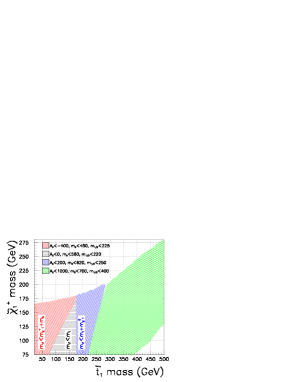
Figure 1: Kinematical regions in the $m_{{\tilde{t}}_{1}}$–$m_{{\tilde{\chi}}_{1}^{+}}$ plane. From left to right: Region I $m_{\tilde{t}_{1}}<m_{{\tilde{\chi}}_{1}^{+}}+m_{b}$; Region II $m_{{\tilde{\chi}}_{1}^{+}}+m_{b}<m_{{\tilde{t}}_{1}}<m_{t}$; Region III $m_{t}<m_{{\tilde{t}}_{1}}<m_{{\tilde{\chi}}_{1}^{0}}+m_{t}$; and region IV $m_{{\tilde{t}}_{1}}>m_{{\tilde{\chi}}_{1}^{0}}+m_{t}$

In Appendix A we give the Feynman rules for all vertices involving squarks, quarks, charginos and neutralinos, as well as the two–body squark decay-widths, for squarks of all three generations. These equations reduce to the expressions found in Ref. [37] provided one identifies $\Gamma_{UL}^{33}=\cos\theta_{\tilde{t}}$ and $\Gamma_{UR}^{33}=\sin\theta_{\tilde{t}}$. They also generalize the results for the BRpV model to the three-generation case.

4 Lightest Stop Two-Body Decays in MSUGRA

In an R–parity conserving supergravity theory the main $\tilde{t}_{1}$ decay channel expected in region I of Fig. 1 is the loop–induced and flavour–changing $\tilde{t}_{1}\to c\,\tilde{\chi}_{1}^{0}$  [19, 20, 21]. As is well-known, the FCNC processes in the MSSM in general involve a very large number of input parameters. For this reason, following common practice, we prefer to perform the phenomenological study of flavour changing processes in the framework of a supergravity theory with universal supersymmetry breaking. The simplest description of FCNC processes in R-parity conserving minimal SUGRA models uses the so-called one-step approximation. Here we start by reproducing the standard calculation for $\tilde{t}_{1}\to c\,\tilde{\chi}_{1}^{0}$ as in [19]. To do this consider only the effect of the third generation Yukawa coupling. From our general eq. (A.10) we have for $\tilde{t}_{1}=\tilde{u}_{l}$

$$\Gamma(\tilde{t}_{1}\to c\,\tilde{\chi}_{1}^{0})\approx\frac{g^{2}}{8\pi}\left(\Gamma_{UL13}\right)^{2}\left[{\hbox{$\frac{2}{3}$}}\sin\theta_{W}N^{\prime}_{11}+\left({\hbox{$\frac{1}{2}$}}-{\hbox{$\frac{2}{3}$}}\sin^{2}\theta_{W}\right)\frac{N^{\prime}_{12}}{\cos\theta_{W}}\right]^{2}m_{\tilde{t}_{1}}\left(1-\frac{m_{\tilde{\chi}_{1}^{0}}^{2}}{m_{\tilde{t}_{1}}^{2}}\right)^{2}$$ (35)

with

$$\Gamma_{UL13}=\frac{\Delta_{L}\cos\theta_{\tilde{t}}-\Delta_{R}\sin\theta_{\tilde{t}}}{m_{\tilde{c}_{L}}^{2}-m_{\tilde{t}_{L}}^{2}}$$ (36)

In the one–step approximation $\Delta_{L},\Delta_{R}$ are given by

$$\Delta_{L} = (\tilde{M}_{U}^{2})_{23}\approx(M_{Q}^{2})_{23}\approx-\frac{t_{U}}{16\pi^{2}}K_{cb}K_{tb}h_{b}^{2}(M_{Q}^{2}+M_{D}^{2}+m_{H_{1}}^{2}+A_{b}^{2})$$ (37)

$$\Delta_{R} = (\tilde{M}_{U}^{2})_{26}\approx(A_{U}^{h})_{23}\approx-\frac{t_{U}}{16\pi^{2}}K_{cb}K_{tb}h_{b}^{2}m_{t}(A_{b}+\frac{1}{2}A_{t})$$ (38)

with $t_{U}=\ln(M_{G}/m_{t})$. So, in the one–step approximation we have

$$\Gamma(\tilde{t}_{1}\to c\,\tilde{\chi}_{1}^{0})\approx Fh_{b}^{4}(\delta_{m_{0}^{2}}\cos\theta_{\tilde{t}}-\delta_{A}\sin\theta_{\tilde{t}})^{2}\left[\frac{\sqrt{2}}{6}(\tan\theta_{W}\,N_{11}+3N_{12})\right]^{2}m_{\tilde{t}_{1}}\left(1-\frac{m_{\tilde{\chi}_{1}^{0}}^{2}}{m_{\tilde{t}_{1}}^{2}}\right)^{2}$$ (39)

where the pre–factor $F=\frac{g^{2}}{16\pi}\left(\frac{t_{U}}{16\pi^{2}}K_{cb}K_{tb}\right)^{2}\sim 6\times 10^{-7}$ and the parameter $\delta_{m_{0}^{2}}$ is given by

$$\delta_{m_{0}^{2}}=\frac{M_{Q}^{2}+M_{D}^{2}+m_{H_{1}}^{2}+A_{b}^{2}}{m_{\tilde{c}_{L}}^{2}-m_{\tilde{t}_{L}}^{2}}\sim 1$$ (40)

is basically independent of the initial conditions due to the $m_{0}$ dependence both in the numerator as in the denominator and

$$\delta_{A}=\frac{m_{t}(A_{b}+\frac{1}{2}A_{t})}{m_{\tilde{c}_{L}}^{2}-m_{\tilde{t}_{L}}^{2}}$$ (41)

Note however, that the one-step approximation includes only the third generation Yukawa couplings and neglects the running of the soft breaking terms [19, 20, 21, 22]. Such an approximation is rather poor for our purposes, since we will be interested in comparing with R-parity violating decay modes (see the next section). In order to have an accurate calculation of the respective branching ratios we need to go beyond the one-step approximation. We therefore use a exact numerical calculation for the FCNC process $\tilde{t}\to c\,\tilde{\chi}_{1}^{0}$ in which the running of the Yukawa couplings and soft breaking terms is taken into account. First we have checked that indeed the effect of the Yukawas from the two first generations is negligible. However the same is not true for the running of the soft breaking terms. As can be seen from Figure 2 the range of variation that we obtain from the numerical solution is

$$\Gamma(\tilde{t}_{1}\to c\,\tilde{\chi}_{1}^{0})\sim(10^{-16}\hbox{ -- }10^{-6})\hbox{GeV}$$ (42)

depending on the assumed value of $m_{1/2}$ and $\tan\beta$. In this figure we have compared the decay width obtained from eq. (A.10) with the approximate formulae in eq. (35) for two fixed values of $m_{1/2}$, $\tan\beta$ and taking $A_{0}=0$. The approximate formulae only reproduce well the numerical result for the academic case of no SUSY breaking gaugino mass, $m_{1/2}=0$. For the more realistic case $m_{1/2}>100\,$GeV, the exact solution is usually one decade smaller than the approximate one. In the one-step approximation $\Gamma(\tilde{t}_{1}\to c\,\tilde{\chi}_{1}^{0})$ can be arbitrarily small if the two terms $\delta_{m_{0}^{2}}\cos\theta_{\tilde{t}}$ and $\delta_{A}\sin\theta_{\tilde{t}}$ in eq. (39) cancel. This behaviour can be illustrated in Figure 2 by the dashed line labelled 358, which corresponds to $m_{0}=358$ GeV. One sees clearly that while the approximate solution goes to zero, the numerical one reaches a minimum value around $10^{-11}$ GeV. The wrong behaviour of the approximate solution indicates that the $\delta_{A}$ depends strongly on the scale. For example, the RGE for $A_{b}$ is very sensitive on $m_{1/2}$ and $\tan\beta$ and in the one-step approximation there is no explicit dependence on $m_{1/2}$, which is crucial. Both solutions increase with $\tan\beta$, as expected by the bottom Yukawa dependence explicit in eq. (39) and remain practically constant for large $m_{1/2}$ values.

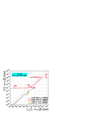
Figure 2: Comparison between the exact numerical calculation (ordinate) and the one–step approximation (abscissa) for the $\tilde{t}_{1}\to c\,\tilde{\chi}_{1}^{0}$ decay width for various values of $\tan\beta$ and $m_{1/2}$ with $A_{0}=0$ and $m_{0}$ varying in the indicated range. The dotted left diagonal line would signify the equality between the estimates, while the right diagonal line would indicate one order of magnitude difference. Results of both estimates indicated in the lower right legend. More details are found in the text.

5 Two-Body Decays of the Lightest Stop: the R-parity violating case

In contrast to the case of an R–parity conserving supergravity theory, in our broken R–parity model one can have a competing R-parity violating stop decay mode in region I of Fig. 1. From eq. (A.11) with $\tau=F_{3}^{+}$ one can easily compute the R-parity violating stop decay width $\tilde{t}_{1}\to b\,\tau$,

$$\Gamma(\tilde{t}_{1}\to b\,\tau) = \frac{g^{2}\lambda^{1/2}(m_{\tilde{t}_{1}}^{2},m_{b}^{2},m_{\tau}^{2})}{16\pi m_{\tilde{t}_{1}}^{3}}\{-4U_{32}^{*}\hat{h}_{b}c_{\theta_{\tilde{t}}}(V_{32}^{*}\hat{h}_{t}s_{\theta_{\tilde{t}}}-V_{31}^{*}c_{\theta_{\tilde{t}}})m_{b}m_{\tau}$$ (43)

$$+[(V_{32}^{*}\hat{h}_{t}s_{\theta_{\tilde{t}}}-V_{31}^{*}c_{\theta_{\tilde{t}}})^{2}+U_{32}^{*2}\hat{h}_{b}^{2}c^{2}_{\theta_{\tilde{t}}}](m_{\tilde{t}_{1}}^{2}-m_{b}^{2}-m_{\tau}^{2})\}$$

which coincides with the result found in Ref. [17]. In [38] it was shown that, except for $U_{32}$ which determines the SU(2)-conserving mixing of the Higgsino with the left-handed $\tau$, all other mixing matrix elements $V_{3i}$ and $U_{3i}$ are proportional to $v_{3}^{II}$ and therefore to the tau–neutrino mass. Neglecting these terms we have from eq. (43)

$$\Gamma(\tilde{t}_{1}\to b\,\tau)\approx\frac{g^{2}\lambda^{1/2}(m_{\tilde{t}_{1}}^{2},m_{b}^{2},m_{\tau}^{2})}{16\pi m_{\tilde{t}_{1}}^{3}}\sin^{2}\xi^{\prime}\hat{h}_{b}^{2}c^{2}_{\theta_{\tilde{t}}}(m_{\tilde{t}_{1}}^{2}-m_{b}^{2}-m_{\tau}^{2})$$ (44)

noting that, to a good approximation,

$$|U_{32}|\approx\left|\frac{\epsilon_{3}}{\mu^{\prime}}\right|=|\sin\xi^{\prime}|$$ (45)

where $\epsilon_{3}$ corresponds to the bilinear mass parameter in basis I. The lesson here is that the R-Parity violating decay rate $\Gamma(\tilde{t}_{1}\to b\,\tau)$ is proportional to $\epsilon_{3}$ or, equivalently, to $\sin^{2}\xi^{\prime}$, instead of $\sin^{2}\xi$, and thus not necessarily small, since it is not directly controlled by the neutrino mass. In other words, there can be cancellations in the latter but not in the R-parity violating branching ratio.

The meaning of the factor $\sin^{2}\xi^{\prime}h_{b}^{2}$ may also be seen in basis II, where $\epsilon^{II}_{3}=0$. In this case $v_{3}^{II}$ is proportional to the tau–neutrino mass so that, as already mentioned, in this basis all the elements $U_{3i}$ and $V_{3i}$ are small [26]. Neglecting these terms, $\Gamma(\tilde{t}_{1}\to b\,\tau)$ may be written directly from the interaction term $\tilde{t}_{L}b_{R}\tau_{L}$, which is induced by the trilinear term in the $\epsilon^{II}_{3}=0$–basis given in eq. (10) as

$$\lambda_{3}^{II}=\left(\epsilon_{3}/\mu^{\prime}\right)h_{b}=h_{b}\sin\xi^{\prime}$$ (46)

which is the factor in eq. (44). Note, however, that in our numerical calculation to be described in the next section we have used for $\Gamma(\tilde{t}_{1}\to b\,\tau)$ the full expression given in eq. (A.10) of the appendix.

In the next section we will determine the conditions under which the R-parity violating decay width $\Gamma(\tilde{t}_{1}\to b\,\tau)$ can be dominant over the R-parity conserving ones, $\Gamma(\tilde{t}_{1}\to c\,\tilde{\chi}_{1}^{0})$ and $\Gamma(\tilde{t}_{1}\to b\,\tilde{\chi}_{1}^{+})$.

5.1 Region I

Using the one-step approximation for $\Gamma(\tilde{t}_{1}\to c\,\tilde{\chi}_{1}^{0})$ one finds

$$\Gamma(\tilde{t}_{1}\to c\,\tilde{\chi}_{1}^{0})\sim 10^{-6}h_{b}^{4}m_{\tilde{t}_{1}}\left(1-\frac{m_{\tilde{\chi}_{1}^{0}}^{2}}{m_{\tilde{t}_{1}}^{2}}\right)^{2}$$ (47)

Using the eq. (44) and neglecting charm, tau and bottom masses we get

$$\frac{\Gamma(\tilde{t}_{1}\to c\,\tilde{\chi}_{1}^{0})}{\Gamma(\tilde{t}_{1}\to b\,\tau)}\sim 10^{-5}\frac{h_{b}^{2}}{\sin^{2}\xi^{\prime}}\left(1-\frac{m_{\tilde{\chi}_{1}^{0}}^{2}}{m_{\tilde{t}_{1}}^{2}}\right)^{2}$$ (48)

Therefore $\Gamma(\tilde{t}_{1}\to c\,\tilde{\chi}_{1}^{0})$ will start to compete with $\Gamma(\tilde{t}_{1}\to b\,\tau)$ from $\sin\xi^{\prime}\raise 1.1625pt\hbox{$\;<$\kern-6.75pt\raise-4.2625pt\hbox{$\sim\;$}}5\times 10^{-3}$ ($10^{-4}$) for $\tan\beta$ large (small). In Fig. 3 we compare $BR({\tilde{t}}_{1}\to c\,{\tilde{\chi}_{1}^{0}})$ [calculated numerically from their exact formula in (A.10)] with $BR({\tilde{t}}_{1}\to b\,\tau)$ within the restricted region of the $m_{{\tilde{t}}_{1}}$–$m_{{\tilde{\chi}}_{1}^{0}}$ plane where only those two decay modes are open. We consider different $m_{\nu_{\tau}}$ values (these correspond to relatively small values of the R-parity parameters $|\epsilon_{3}|,|v_{3}|\raise 1.1625pt\hbox{$\;<$\kern-6.75pt\raise-4.2625pt\hbox{$\sim\;$}}1$ GeV). We vary the MSSM parameters randomly obeying the condition $m_{\tilde{t}_{1}}<m_{\tilde{\chi}^{\pm}_{1}}+m_{b}$ and depict the corresponding region in light grey. The upper–left triangular region is defined by kinematics and corresponds to $m_{\tilde{t}_{1}}<m_{\tilde{\chi}^{0}_{1}}+m_{c}$, so that $BR(\tilde{t}_{1}\to b\,\tau)=100\>\%$. The lower–right grey corresponds to $m_{\tilde{t}_{1}}>m_{\tilde{\chi}^{0}_{1}}+m_{c}$ when the sampling is done over the region defined by eq. (3). One notices from Fig. 3 that in the central region the dominant stop decay mode is $\tilde{t}_{1}\to b\,\tau$ with branching ratio $BR(\tilde{t}_{1}\to b\,\tau)>0.9$. The dotted lines in the light grey region indicate maximum $\nu_{\tau}$ mass values obtained in the scan. In the calculation of the $\nu_{\tau}$ mass, we have allowed only up to one order of magnitude of cancellation between the two terms which contribute to $\sin\xi$. Therefore if the lightest stop only decays into the two modes considered here, the processes $\tilde{t}_{1}\to b\,\tau$, will be important even for the case of very light tau–neutrino masses.

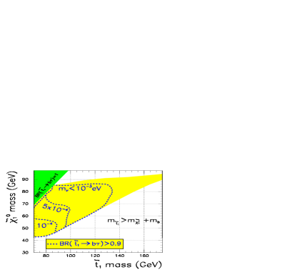
Figure 3: Regions where the ${\tilde{t}}_{1}\to b\,\tau$ decay branching ratio exceeds 90% in the $m_{{\tilde{t}}_{1}}$–$m_{{\tilde{\chi}}_{1}^{0}}$ plane for different $m_{\nu_{\tau}}$ values. The MSSM parameters are randomly varied as indicated in the text under the restriction $m_{\tilde{t}_{1}}<m_{\tilde{\chi}^{\pm}_{1}}+m_{b}$. The upper–left triangular region corresponds to $m_{\tilde{t}_{1}}<m_{\tilde{\chi}^{0}_{1}}+m_{c}$ so that only the $\tilde{t}_{1}\to b\,\tau$ decay channel is open. The lower–right unshaded region corresponds to $m_{\tilde{t}_{1}}>m_{\tilde{\chi}^{+}_{1}}+m_{b}$.

We note however that we can use the limits obtained from leptoquark searches [39] in order to derive limits on the top-squark for our R-parity violating case. In particular, if $BR({\tilde{t}}_{1}\to b\tau)=1$ stop masses less than 99 GeV are excluded at 95% of CL., under the assumption that the three–body decays of the stops are negligible. Therefore, the dark region in Fig. 3 would be ruled out. In ref. [40] we have determined the corresponding restrictions on the SUGRA parameter space.

The dependence on the tau neutrino mass may be seen in Fig. 4 where the role played by $\tan\beta$ is manifest. In this figure we have shown $BR(\tilde{t}_{1}\to b\,\tau)$ as function of the lighter stop mass for tau–neutrino mass in the sub–eV range, indicated by the simplest oscillation interpretation of the Super-Kamiokande atmospheric neutrino data. We have obtained such tau–neutrino mass values numerically, allowing only one decade of cancellation between the two terms that contribute to $\sin\xi$ in eq. (20). The degree of suppression for $\epsilon_{3}/\mu$ obtained numerically agrees very well with the expectations from the approximate formula for the minimal tau–neutrino mass in eq. (23). In contrast with Ref. [17], in our case $BR({\tilde{t}}_{1}\to b\tau)$ decreases with $\tan\beta$. The reason for this difference is that here we take into account the fact that the mixing parameter $\Gamma_{UL13}$ obtained from the RGE depends on $h_{b}^{2}$ in eq. (35), while in ref. [17] was simply regarded as a phenomenological input parameter (called $\delta$ there).

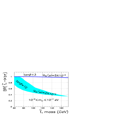
Figure 4: $BR(\tilde{t}_{1}\to b\,\tau)$ as function of the lighter stop mass for tau–neutrino mass in the sub–eV range and two different values of $\tan\beta$ and $\epsilon_{3}/\mu$. This prediction is natural in the sense that we have allowed only up to one order of magnitude of cancellation between the two terms that contribute to $\sin\xi$.

The message from this subsection is that in our SUGRA R-parity violating model the R-Parity violating decay mode $\tilde{t}_{1}\to b\,\tau$ can very easily dominate the R-Parity conserving decay mode $\tilde{t}_{1}\to c\,\tilde{\chi}_{1}^{0}$, even for very small neutrino masses.

5.2 Region II

In region II the R–Parity conserving decay mode $\tilde{t}_{1}\to b\tilde{\chi}^{+}_{1}$ is open (but not $\tilde{t}_{1}\to t\nu$), and competes with the R–Parity violating mode $\tilde{t}_{1}\to b\,\tau$. Replacing the subindex 3 by 1 on the diagonalization matrices $U$ and $V$ in eq. (43) we get the corresponding expression for $\Gamma(\tilde{t}_{1}\to b\,\tilde{\chi}_{1}^{+})$. In order to get an approximate expression for the ratio of the two main decay rates in this region, we note that in MSUGRA the lightest chargino is usually gaugino-like, implying that $V_{11}^{2}\sim 1$. In addition, the lightest stop is usually right-handed, hence $\sin^{2}\theta_{\tilde{t}}\raise 1.1625pt\hbox{$\;>$\kern-6.75pt\raise-4.2625pt\hbox{$\sim\;$}}\cos^{2}\theta_{\tilde{t}}$. This way we find

$$\frac{\Gamma(\tau)}{\Gamma(\tilde{\chi}_{1}^{+})}\equiv\frac{\Gamma(\tilde{t}_{1}\to b\,\tau)}{\Gamma(\tilde{t}_{1}\to b\,\tilde{\chi}_{1}^{+})}\approx\frac{\sin^{2}\xi^{\prime}\hat{h}_{b}^{2}\cos^{2}{\theta_{\tilde{t}}}}{\left[(V_{11}^{*}\cos{\theta_{\tilde{t}}}-V_{12}^{*}\hat{h}_{t}\sin{\theta_{\tilde{t}}})^{2}+U_{12}^{*2}\hat{h}_{b}^{2}\cos^{2}{\theta_{\tilde{t}}}\right]}\,K$$ (49)

where $K$ is a kinematical factor depending on the lightest stop and chargino masses, and here we have defined $\hat{h}_{t,b}\equiv h_{t,b}/g$. The presence of the bottom quark Yukawa coupling indicates that large values of $\tan\beta$ are necessary to have large R–Parity violating branching ratios in this region. In fact, we have checked numerically with the exact expressions that in Region II (RII) ${\Gamma(\tau)}/{\Gamma(\tilde{\chi}_{1}^{+})}\raise 1.1625pt\hbox{$\;>$\kern-6.75pt\raise-4.2625pt\hbox{$\sim\;$}}1$ only for large $\tan\beta$ as we will see in the next figures.

In Fig. 5 we show the regions in the $m_{\chi^{\pm}_{1}}-m_{\tilde{t}_{1}}$ plane where $BR(\tilde{t}_{1}\to b\,\tau)$ dominates over $BR(\tilde{t}_{1}\to b\widetilde{\chi}^{+}_{1})$. In the upper–left region the decay mode $\tilde{t}_{1}\to b\widetilde{\chi}^{+}_{1}$ is not allowed and corresponds to Region I. Below and to the right of this zone, and above and to the left of three rising lines, lies region RII where ${\Gamma(\tau)}/{\Gamma(\tilde{\chi}_{1}^{+})}>1$. The three lines correspond to $|\epsilon_{3}|<80$ GeV (dashed), $|\epsilon_{3}|<60$ GeV (dotted), and $|\epsilon_{3}|<40$ GeV (dot–dashed), respectively. The proximity to the upper-left zone indicates that the RPV decay dominates only close to the threshold where there is a high kinematical suppression of the R–parity-conserving one, through the factor $K$. Unlike the case of region I this requires large values of the RPV parameters. Note, moreover, that if the stops have a small mixing ($\cos{\theta_{\tilde{t}}}\approx 0$), then ${\Gamma(\tau)}/{\Gamma(\tilde{\chi}_{1}^{+})}\ll 1$ in RII.

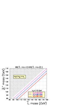
Figure 5: Contours of $BR({\tilde{t}}_{1}\to b\,\tau)>BR({\tilde{t}}_{1}\to b\tilde{\chi}_{1}^{+})$ in the $m_{{\tilde{t}}_{1}}$–$m_{{\tilde{\chi}}_{1}^{+}}$ plane for $|v_{3}|<10$ GeV. Three different maximum values for $|\epsilon_{3}|$ are considered: $|\epsilon_{3}|<40$ GeV (dot-dash), $|\epsilon_{3}|<60$ GeV (dots), and $|\epsilon_{3}|<80$ GeV (dashes). The region where $m_{\tilde{t}_{1}}<m_{b}+m_{\widetilde{\chi}^{+}_{1}}$ corresponds to the previously studied Region I.

A simpler expression for the ratio of decay rates in eq. (49) is obtained if we take $V_{11}\approx 1$ and assume no kinematical suppression in eq. (49) through the factor $K$:

$$\frac{\Gamma(\tau)}{\Gamma(\tilde{\chi}_{1}^{+})}\sim\sin^{2}\xi^{\prime}\hat{h}_{b}^{2}\,.$$ (50)

Note that the presence of the parameter $\sin\xi^{\prime}=\epsilon_{3}/\mu^{\prime}$ indicates that the R–Parity violating decay mode is not strictly proportional to the neutrino mass, but proportional to the BRpV parameter $\epsilon_{3}^{2}$.

However generically we expect some correlation with the $\nu_{\tau}$ mass, especially in the case where the boundary conditions in the RGE are universal and there are no strong cancellations between two terms that contribute to $\sin\xi$ as shown in Fig. 6. In this figure we plot the ratio $\Gamma(\tau)/\Gamma(\tilde{\chi}_{1}^{+})$ in RII as a function of the tau–neutrino mass. Both decay rates have been calculated numerically from the exact formulas. In this figure we have imposed both $m_{H_{1}}^{2}=M_{L}^{2}$ and $B=B_{3}$ within 0.1% at the GUT scale. Cancellation between the $\Delta m^{2}$ and $\Delta B$ terms in the neutrino mass formula of eq. (20) are accepted only within 1 decade. As a reference we have drawn the line corresponding to $\Delta B=0$ and $\Delta m^{2}=\Delta m^{2}_{min}$ ($\Delta m^{2}$ is negative and its magnitude is bounded from below by $\Delta m^{2}_{min}$) at the weak scale, which gives an idea of the value of the neutrino mass when there is no cancellation between the $\Delta B$ and $\Delta m^{2}$ terms.

We have imposed an upper bound on $m_{\nu_{\tau}}$ at the collider experimental limit of the tau–neutrino mass, and have chosen fixed values of $\epsilon_{3}/\mu=1$, 0.1, and 0.01. The allowed region for $\epsilon_{3}/\mu=1$ is above the dashed line. In the case of $\epsilon_{3}/\mu=0.1$ (0.01) the allowed region lies enclosed between the solid (dotted) lines. The effect of $\tan\beta$ is to increase the ratio $\Gamma(\tau)/\Gamma(\tilde{\chi}_{1}^{+})$: the minimum value of the ratio is obtained for $\tan\beta\approx 2$ and the maximum corresponds to $\tan\beta\approx 60$. The extreme values of $\tan\beta$ are dictated by perturbativity.

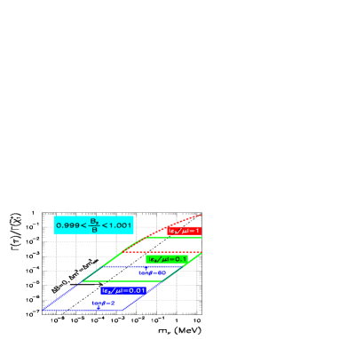
Figure 6: Regions for $\Gamma({\tilde{t}}_{1}\to b\,\tau)/\Gamma({\tilde{t}}_{1}\to b\,{\tilde{\chi}_{1}^{+}})$ as a function of the tau–neutrino mass with the universality condition $B=B_{3}$ at the unification scale imposed at the 0.1% level as indicated. Its effect is to alter the maximum attainable tau–neutrino mass. The dot-dashed line corresponds to the case where $\Delta B=0$ at the weak scale.

A number of statistically less significant points appear outside the drawn regions in Fig. 6 and are not depicted. They correspond to points with $m_{\tilde{t}_{1}}-m_{b}-m_{{\tilde{\chi}}_{1}^{\pm}}<10\,$ GeV which appear above the diagonal line, and points with $\cos\theta_{\tilde{t}}<0.1$ which appear below the horizontal line corresponding to the lowest values of $\tan\beta$. In the last case, our approximation in eq. (50) does not work any more. On the other hand, eq. (50) predicts very well the behavior of $\Gamma(\tau)/\Gamma(\tilde{\chi}_{1}^{+})$ if $\cos\theta_{\tilde{t}}>0.1$. For example for $\epsilon_{3}/\mu=1$, or equivalently $\sin\xi^{\prime}=1/\sqrt{2}$, we expect from eq. (50) a maximum value of order 1 for large $\tan\beta$ ($h_{b}\approx 1$) and a minimum value of order $10^{-3}$ for small $\tan\beta$ ($h_{b}^{2}\approx 10^{-3}$), and this is confirmed by Fig. 6. High values of the R–parity violating branching ratio for large $\epsilon_{3}$ values are highly restricted for large $\tan\beta$. This can be understood as follows. In the case of $\epsilon_{3}/\mu=1$ and $\tan\beta=60$ acceptable neutrino masses are obtained only if $\sin\xi\sim 1$. On the other hand, in this regime we find from eq. (20) that the $\Delta B$ term is large because of the high value of $\tan\beta$, and that the $\Delta m^{2}$ term is large because $m_{H_{1}}^{2}$ becomes negative and $\Delta m^{2}=m_{H_{1}}^{2}-M_{L}^{2}$ grows in magnitude. This way, acceptable neutrino masses are achieved only with cancellation within more than one decade. In any case, we think that Fig. 6 is very conservative considering that in MSSM–SUGRA with unification of top-bottom-tau Yukawa couplings, the large value of $\tan\beta$ implies that a cancellation of four decades among vev’s is needed.

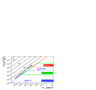
Figure 7: Regions for $\Gamma({\tilde{t}}_{1}\to b\,\tau)/\Gamma({\tilde{t}}_{1}\to b\,{\tilde{\chi}_{1}^{+}})$ as a function of the tau–neutrino mass for different levels of cancellation between the two terms that contribute to the neutrino mass. We impose the universality condition $m_{H_{1}}^{2}=M_{L}^{2}$ at the unification scale, but $B$ and $B_{3}$ are not universal. We take $|\epsilon_{3}/\mu|=1$ (inside the dashed lines), $|\epsilon_{3}/\mu|=0.1$ (solid lines), and $|\epsilon_{3}/\mu|=0.01$ (dotted lines).

The width of the band in Fig. 6 reflects the degree of correlation between the ratio $\Gamma({\tilde{t}}_{1}\to b\,\tau)/\Gamma({\tilde{t}}_{1}\to b\,{\tilde{\chi}_{1}^{+}})$ and the neutrino mass under the mentioned conditions. Note that one would have an indirect measurement of the neutrino mass if this ratio were determined independently. The band will open to the left if one allows a stronger cancellation between the terms in $\Delta B$ and $\Delta m^{2}$. On the other hand it will open to the right if the universality between $B$ and $B_{3}$ is relaxed. This is shown in Fig. 7 where we plot the ratio $\Gamma(\tau)/\Gamma(\tilde{\chi}_{1}^{+})$ in RII as a function of the tau–neutrino mass, but without imposing universality between $B_{3}$ and $B$. If we accept cancellation within one decade between the $\Delta B$ and $\Delta m^{2}$ terms , then the allowed region is at the right and below the corresponding dashed tilted line. If a larger degree of cancellation is accepted, the left boundary of the allowed region moves to the left as indicated in the figure, enhancing the R-parity violating channel. In addition if we accept only a decade of cancellation between the two terms that contribute to the tau–neutrino mass, then our approximate formula which predicts the minimum tau–neutrino mass in eq. (23) works very well.

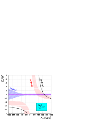
Figure 8: Universality condition $B=B_{3}$ at the unification scale as a function of $A_{0}$. As $\tan\beta$ increases, the allowed values of $A_{0}$ are more constrained.

In summary, in this subsection we have shown that even in region II, where the R-Parity conserving decay mode ${\tilde{t}}_{1}\to b\,{\tilde{\chi}_{1}^{+}}$ is also open, the R-Parity violating decay mode ${\tilde{t}}_{1}\to b\,\tau$ can be comparable to ${\tilde{t}}_{1}\to b\,{\tilde{\chi}_{1}^{+}}$ for large $\tan\beta$ and $\epsilon_{3}$, and relatively close to the chargino production threshold. In general, this implies a large neutrino mass unless a cancellation is accepted between the two terms contributing to the tree level neutrino mass. In addition, the non-universality of the $B$ and $B_{3}$ terms at the GUT scale does not increase appreciably the allowed parameter space, except at large $\tan\beta$. The main consequence of this non-universality is to restrict the allowed values of $A_{0}$ at large $\tan\beta$. In the next subsection we study the effects introduced by the non-universality of $m_{H_{1}}^{2}$ and $m_{L_{3}}^{2}$.

5.3 Effects of non–Universality

We now study the effect of possible non-universality of soft-breaking SUSY parameters on our previous results. In particular, the non-universality between $m_{H_{1}}^{2}$ and $m_{L_{3}}^{2}$ at the GUT scale. The Minimal SUGRA model, while highly predictive, rests upon a number of simplifying assumptions which do not necessarily hold in specific models due to the possible evolution of the physical parameters in the range from $M_{Planck}$ to $M_{GUT}$. Specifically, there are several models in the literature with non-universal soft SUSY breaking mass parameters at high scales. A recent survey can be found in [41], where several models such as based on string theory, M-theory, and anomaly mediated supersymmetry are analyzed. For this reason we find interesting to explore here the effects of non-universal soft terms.

The SUGRA spectra are typically found for given values of $m_{1/2}$, $m_{0}$, $A_{0}$, $\tan\beta$ and Sgn($\mu$). In our case we have in addition $\sin\xi^{\prime}$ (or equivalently, $\epsilon_{3}$). The value of $v_{3}$ is determined by the previous parameters through the minimization conditions. In addition, a relation between $A_{0}$ and the ratio $B_{3}/B$ at the GUT scale (which indicates the degree of universality) emerges. This relation can be seen in Fig. 8 for $\epsilon_{3}/\mu=1$ and the values $\tan\beta=3$, 40, and 60, for $m_{H_{1}}^{2}=M_{L}^{2}$. The relation becomes more restrictive as $\tan\beta$ is increased, starting from $-1000<A_{0}<1000$ GeV allowed for $\tan\beta=3$, to a single $A_{0}$ value compatible with unification for $\tan\beta=60$.

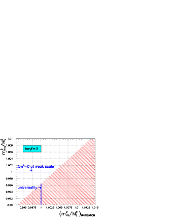
Figure 9: Comparison between the ratio $m_{H_{1}}^{2}/M_{L}^{2}$ at the weak and the unification scales for $\tan\beta=3$. Universality at the unification scale, $m_{H_{1}}^{2}/M_{L}^{2}=1$, implies a maximum value for this ratio at the weak scale.

Another way to enhance the R-parity violating channel, enlarging the band towards the left in Fig. 6, is by relaxing the universality between $m_{H_{1}}^{2}$ and $M_{L}^{2}$ at the GUT scale. In Fig. 9 we plot the ratio $m_{H_{1}}^{2}/M_{L}^{2}$ at the weak scale as a function of the same ratio at the unification scale $M_{GUT}$ for $\tan\beta=3$. The shaded region is allowed, implying a maximum value for the ratio $m_{H_{1}}^{2}/M_{L}^{2}$ at the weak scale for a given value of the ratio at the GUT scale. We see from Fig. 9 that a relaxation of universality of 0.5% or more is enough to make $(m_{H_{1}}^{2}/M_{L}^{2})_{weak}=1$ possible, meaning that smaller neutrino masses are attainable without having to rely on a cancellation between the $\Delta m^{2}$ and $\Delta B$ terms or small values of $\Gamma({\tilde{t}}_{1}\to b\tau)$.

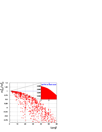
Figure 10: $(m_{H_{1}}^{2}/M_{L}^{2})$ evaluated at the weak scale as a function of $\tan\beta$. This ratio is always less than one and decreases with $\tan\beta$.

However as we increase $\tan\beta$ the maximum value of $m_{H_{1}}^{2}/M_{L}^{2}$ decreases, and thus, the required non-universality between $m_{H_{1}}$ and $M_{L}$ at unification scale grows drastically. In Fig. 10 we show the ratio $m_{H_{1}}^{2}/M_{L}^{2}$ at the weak scale as a function of $\tan\beta$. We appreciate clearly the growing of $|\Delta m^{2}|_{min}$ with $\tan\beta$. We remind the reader that this kind of non–universality in the soft terms is not uncommon in string models [42], or GUT models based on $SU(5)$ [43] or $SO(10)$ [44] for example. There are in fact some $SO(10)$ models for non-universality of the GUT scale scalar masses which naturally favour light neutrino mass [44].

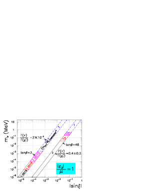
Figure 11: Minimum value of the tau–neutrino mass as a function of $\sin\xi$ for different values of $m_{H_{1}}/M_{L}$ at the GUT scale and two values of $\tan\beta$. The ratio $\epsilon_{3}/\mu$ is fixed to the indicated value, leading to a nearly constant value for $\Gamma({\tilde{t}}_{1}\to b\,\tau)/\Gamma({\tilde{t}}_{1}\to b\,{\tilde{\chi}_{1}^{+}})$. Here we assume that the two terms contributing to the tau–neutrino mass cancel to within an order of magnitude.

The effect of non–universality it is also explored in Fig. 11 where it is shown the relation between the neutrino mass and the parameter $\sin\xi$ for $\epsilon_{3}/\mu=1$. Two different bands are shown: one for $\tan\beta=3$ and $\Gamma(\tau)/\Gamma(\tilde{\chi}_{1}^{+})=2\times 10^{-3}$, and a second one for $\tan\beta=46$ and $\Gamma(\tau)/\Gamma(\tilde{\chi}_{1}^{+})=0.4\pm 0.2$. The required degree of universality at the GUT scale is indicated inside the bands. For example, in order to have neutrino masses of the order of eV for $\tan\beta=3$, $m_{H_{1}}^{2}$ needs to be at least 0.2% larger than $M_{L}^{2}$. Similarly, for $\tan\beta=46$ we need a $m_{H_{1}}^{2}$ twice as large as $M_{L}^{2}$ at the GUT scale in order to have neutrino masses of 1 eV. We stress the fact that for Fig. 11 we have conservatively accepted cancellation at the level of one order-of-magnitude only.

In summary, the lesson to learn here is that non-universal soft SUSY breaking terms at the GUT scale have the potential of making it easier to reconcile sizeable R-Parity violating effects in the stop sector with very small neutrino masses, without resorting to cancellations.

6 Conclusions

We have studied the decays of the lightest top squark in SUGRA models with and without R-parity. We have improved the calculation for the decay $\tilde{t}_{1}\to c\,\tilde{\chi}^{0}$ by numerically solving the renormalization group equations (RGE’s) of the MSSM including full generation mixing in the RGE’s for Yukawa couplings as well as soft SUSY breaking parameters. The decay-width is in general one order of magnitude smaller than the one obtained in the usual one–step approximation. This result will therefore enlarge the regions of parameter space where the four–body decays of lightest stop dominate over the decay into a charm quark and the lightest neutralino. As a result it will affect the present experimental lower bound on the $\tilde{t}_{1}$ mass even in the R-parity conserving case [22]. If R–parity breaks of course new decay modes appear and, as we have shown, they can be sizeable. In fact we have shown that the lightest stop can be the LSP, decaying with 100% rate into a bottom quark and a tau lepton. We have shown that the decay mode $\tilde{t}_{1}\to b\,\tau$ dominates over $\tilde{t}_{1}\to c\,\tilde{\chi}^{0}$ even for neutrino masses in the range suggested by the simplest oscillation interpretation of the Super-Kamiokande atmospheric neutrino data. This result would have a strong impact on the top squark search strategies at LEP [45] and TEVATRON [46], where it is usually assumed that the $\tilde{t}_{1}\to c\,\tilde{\chi}^{0}$ decay mode is the main channel. In addition to the signal of two jets and two taus present when the two produced stops decays through the R-parity violating channel, one expects a plethora of exotic high–multiplicity fermion events arising from neutralino decay, since such decay can happen inside the detector even for the small neutrino masses in the range suggested by the $\nu_{\mu}$ to $\nu_{\tau}$ oscillation interpretation of the atmospheric neutrino anomaly [8]. We have also compared the decay $\tilde{t}_{1}\to b\,\tau$ with the R-parity and flavor conserving mode $\tilde{t}_{1}\to b\,\tilde{\chi}^{+}$ and shown that the rate of the former can be comparable or even bigger than the latter if the tau–neutrino mass and $\tan\beta$ are large. However one may have a sizeable branching of $\tilde{t}_{1}\to b\,\tau$ in the case of suppressed tree level neutrino mass as a result of strong cancellations between the two terms that contribute to $\sin\xi$, or in some regions of parameter space of non-universal SUGRA models with $(m^{2}_{H_{1}}/m^{2}_{L_{3}})_{GUT}\neq 1$. A detailed analysis of the detectability prospects of such related signatures at present and future accelerators lies outside of the scope of the present paper and it will be taken up elsewhere.

Appendix A Feynman Rules

In this Appendix we derive the Feynman rules $F_{j}^{0}q_{i}\tilde{q}_{k}$ (involving a neutralino/tau-neutrino, a quark, and a squark) and $F_{j}^{\pm}q_{i}\tilde{q}^{\prime}_{k}$ (involving a chargino/tau, a quark, and a squark of different electric charge) in the case of three generations and RPV in the third generation. This is a generalization of the Feynman rules contained in [47], which are done for the R–Parity conserving MSSM and for one generation of quarks and squarks.

Following [48] we work in a quark interaction basis where $d_{L,R}=d_{L,R}^{0}$, $u_{L}=Ku_{L}^{0}$, and $u_{R}=u_{R}^{0}$ (we denote $q$ and $q^{0}$ the mass and current eigenstates respectively), as opposed to Ref. [49] where a more general basis is used. In addition, we implement the notation $\tilde{q}_{L,R}\equiv\tilde{q}^{0}_{L,R}$ for the interaction basis.

The starting point is the following piece of the Lagrangian

$${\cal L}_{u\tilde{u}F^{0}} = -g{\bar{u}}_{i}^{0}\Bigg{\{}\sqrt{2}\left[\sin\theta_{W}e_{U}{N^{\prime}}_{J1}+\frac{1}{\cos\theta_{W}}({\textstyle{1\over 2}}-e_{U}\sin^{2}\theta_{W}){N^{\prime}}_{J2}\right]\tilde{u}_{iL}$$ (A.1)

$$+\frac{m^{0U}_{ij}}{\sqrt{2}m_{W}\sin\beta\sin\theta}{N^{\prime}}_{J4}\tilde{u}_{jR}\Bigg{\}}P_{R}F_{J}^{0}$$

$$+g{\bar{u}}^{0}_{i}\Bigg{\{}\sqrt{2}\left[\sin\theta_{W}e_{U}{N^{\prime}}_{J1}^{*}+\frac{1}{\cos\theta_{W}}(-e_{U}\sin^{2}\theta_{W}){N^{\prime}}_{J2}^{*}\right]\tilde{u}_{iR}$$

$$-\frac{m^{0U\dagger}_{ij}}{\sqrt{2}m_{W}\sin\beta\sin\theta}{N^{\prime}}_{J4}^{*}\tilde{u}_{jL}\Bigg{\}}P_{L}F_{J}^{0}+\hbox{h.c.}$$

written in the quark interaction basis. The $5\times 5$ matrix $N^{\prime}$ diagonalizes the neutralino/neutrino mass matrix in the $(\tilde{\gamma},\tilde{Z},\tilde{H}_{1}^{0},\tilde{H}_{2}^{0},\nu_{\tau})$ basis as defined in [35], with the index $J=1...5$. The $3\times 3$ up–type quark mass matrix $m^{0U}$ is not diagonal, with the indexes $i,j=1,2,3$.

In order to write the above Lagrangian with mass eigenstates we use the basic relations mentioned before, in particular, $u_{iL}^{0}=(K^{\dagger})^{ij}u_{jL}$, which implies that ${\bar{u}}_{iL}^{0}={\bar{u}}_{jL}K^{ji}$. We need the following relations:

$${\bar{u}}_{iL}^{0}\tilde{u}_{iL} = {\bar{u}}_{iL}\left(\Gamma_{UL}^{*}{(K^{\dagger})}^{*}\right)^{ki}\tilde{u}_{k}$$

$${\bar{u}}_{iL}^{0}m^{0U}_{ij}\tilde{u}_{jR} = {\bar{u}}_{iL}(\Gamma_{UR}^{*}m^{U})^{ki}\tilde{u}_{k}$$

$${\bar{u}}_{iR}\tilde{u}_{iR} = {\bar{u}}_{iR}\Gamma_{UR}^{*ki}\tilde{u}_{k}$$ (A.2)

$${\bar{u}}_{iR}m^{0U}_{ij}\tilde{u}_{jL} = {\bar{u}}_{iR}(\Gamma_{UL}^{*}K^{*}{m}^{U})^{ki}\tilde{u}_{k}$$

where $i,j=1,2,3$ label the quark flavours, $k=1...6$ labels the squarks, and $m^{U}\equiv{\mathrm{diag}}\,\{m_{u},m_{c},m_{t}\}$ is the diagonal up–type quark mass matrix. In this way, the Lagrangian in eq. (A.1) can be written as

$${\cal L}_{u\tilde{u}F^{0}}=-g{\bar{u}}_{i}[(\sqrt{2}G_{0UL}^{*jki}+H_{0UR}^{*jki})P_{R}-(\sqrt{2}G_{0UR}^{*jki}-H_{0UL}^{*jki})P_{L}]F_{j}^{0}\tilde{u}_{k}+\hbox{h.c.}$$ (A.3)

where the different couplings are

$$G_{0UL}^{jki} = \left[\sin\theta_{W}e_{U}{N^{\prime}}^{*}_{j1}+\frac{1}{\cos\theta_{W}}({\textstyle{1\over 2}}-e_{U}\sin^{2}\theta_{W}){N^{\prime}}^{*}_{j2}\right]\left(\Gamma_{UL}K^{\dagger}\right)^{ki}$$

$$G_{0UR}^{jki} = \left[\sin\theta_{W}e_{U}{N^{\prime}}_{j1}+\frac{1}{\cos\theta_{W}}(-e_{U}\sin^{2}\theta_{W}){N^{\prime}}_{j2}\right]\Gamma_{UR}^{ki}$$ (A.4)

$$H_{0UL}^{jki} = {N^{\prime}}_{j4}(\Gamma_{UL}K^{\dagger}{\hat{h}}_{U})^{ki}$$

$$H_{0UR}^{jki} = {N^{\prime}}^{*}_{j4}(\Gamma_{UR}\hat{h}_{U})^{ki}$$

and $\hat{h}_{U}\equiv$diag$\,(m_{u},m_{c},m_{t})/(\sqrt{2}m_{W}\sin\beta\sin\theta)$. Graphically, the $F_{j}^{0}u_{i}\tilde{u}_{k}$ Feynman rules are given by

$-ig[(\sqrt{2}G_{0UL}^{jki}+H_{0UR}^{jki})P_{L}-(\sqrt{2}G_{0UR}^{jki}-H_{0UL}^{jki})P_{R}]$

$-ig[(\sqrt{2}G_{0UL}^{*jki}+H_{0UR}^{*jki})P_{R}-(\sqrt{2}G_{0UR}^{*jki}-H_{0UL}^{*jki})P_{L}]$
The analogous Feynman rules in the MSSM are obtained by replacing $F_{i}^{0}\to\tilde{\chi}^{0}_{i}$, by interpreting the matrix $N$ as the usual $4\times 4$ neutralino mixing matrix, and by setting $\theta=\pi/2$ in the formula for the Yukawa couplings.

Similarly, replacing all $u(\tilde{u})$ by $d(\tilde{d})$ in eq. (A.1) and starting from

$${\cal L}_{q\tilde{q}^{\prime}F^{+}} = g\bar{d}_{i}\left[\frac{m^{0U\dagger}_{ij}}{\sqrt{2}m_{W}\sin\beta\sin\theta}V_{J2}\tilde{u}_{jR}-V_{J1}\tilde{u}_{iL}\right]P_{R}F^{c}_{J}$$ (A.5)

$$+g\bar{d}_{i}\frac{m^{D}_{ij}}{\sqrt{2}m_{W}\cos\beta\sin\theta}U^{*}_{J2}\tilde{u}_{jL}P_{L}F^{c}_{J}$$

$$+g\bar{u}^{0}_{i}\left[\frac{m^{D\dagger}_{ij}}{\sqrt{2}m_{W}\cos\beta\sin\theta}U_{J2}\tilde{d}_{jR}-U_{J1}\tilde{d}_{iL}\right]P_{R}F^{+}_{J}$$

$$+g\bar{u}^{0}_{i}\frac{m^{0U}_{ij}}{\sqrt{2}m_{W}\cos\beta\sin\theta}V^{*}_{J2}\tilde{b}_{jL}P_{L}F^{+}_{J}+\hbox{h.c}$$

we can obtain the complete Feynman rules for the neutralino/tau–neutrino and chargino/tau with quarks and squarks. The results, that complements the obtained in [48], are

Neutralino–(d)quark–(d)squark

$-ig[(\sqrt{2}G_{0DL}^{jki}+H_{0DR}^{jki})P_{L}-(\sqrt{2}G_{0DR}^{jki}-H_{0DL}^{jki})P_{R}]$

$-ig[(\sqrt{2}G_{0DL}^{*jki}+H_{0DR}^{*jki})P_{R}-(\sqrt{2}G_{0DR}^{*jki}-H_{0DL}^{*jki})P_{L}]$

The mixing matrices $G_{0D}$ and $H_{0D}$ are defined as

$$G_{0DL}^{jki} = \left[\sin\theta_{W}e_{D}{N^{\prime}}_{j1}^{*}+\frac{1}{\cos\theta_{W}}(T_{3D}-e_{D}\sin^{2}\theta_{W}){N^{\prime}}^{*}_{j2}\right]\Gamma_{DL}^{ki}$$

$$G_{0DR}^{jki} = \left[\sin\theta_{W}e_{D}{N^{\prime}}_{j1}+\frac{1}{\cos\theta_{W}}(-e_{D}\sin^{2}\theta_{W}){N^{\prime}}_{j2}\right]\Gamma_{DR}^{ki}$$

$$H_{0DL}^{jki} = {N^{\prime}}_{j3}(\Gamma_{DL}{\hat{h}}_{D})^{ki}$$

$$H_{0DR}^{*jki} = {N^{\prime}}_{j3}^{*}(\Gamma_{DR}\hat{h}_{D})^{ki}$$ (A.6)

Chargino/tau–(d)quark–(u)squark

$-ig(-C^{-1})[(G_{UL}^{jki}-H_{UR}^{jki})P_{L}-H_{UL}^{jki}P_{R}]$

$-ig[(G_{UL}^{*jki}-H_{UR}^{*jki})P_{R}-H_{UL}^{*jki}P_{L}]C$

where $C$ is the charge conjugation matrix (in spinor space) and the mixing matrices $G_{U}$ and $H_{U}$ are defined as

$$G_{UL}^{jki} \equiv V_{j1}^{*}\Gamma_{UL}^{ki},\qquad H_{UL}^{jki}\equiv U_{j2}^{*}(\Gamma_{UL}\hat{h}_{D})^{ki},$$

$$H_{UR}^{jki} \equiv V_{j2}^{*}(\Gamma_{UR}\hat{h}_{U}K)^{ki},$$ (A.7)

Chargino/tau–(u)quark–(d)squark

$-ig(-C^{-1})[(G_{DL}^{jki}-H_{DR}^{jki})P_{L}-H_{DL}^{jki}P_{R}]$

$-ig[(G_{DL}^{*jki}-H_{DR}^{*jki})P_{R}-H_{DL}^{*jki}P_{L}]C$

where the mixing matrices $G_{D}$ and $H_{D}$ are defined as

$$G_{DL}^{jki} \equiv U_{j1}^{*}(\Gamma_{DL}K^{\dagger})^{ki},\qquad H_{DL}^{jki}\equiv V_{j2}^{*}(\Gamma_{DL}K^{\dagger}\hat{h}_{U})^{ki},$$

$$H_{DR}^{jki} \equiv U_{j2}^{*}(\Gamma_{DR}\hat{h}_{D}K^{\dagger})^{ki},$$ (A.8)

In order to derive the decays widths we write, for example eq. (A.3) as

$${\cal L}_{u\tilde{u}F^{0}}=g{\bar{u}}_{i}^{0}(f^{*jki}_{U}P_{R}+h^{*jki}_{U}P_{L})F_{j}^{0}\tilde{u}_{k}+\hbox{h.c}$$ (A.9)

The result is

$$\Gamma(\tilde{q}_{k}\to q_{i}+F_{j}^{0}) = \frac{g^{2}\lambda^{1/2}(m_{\tilde{q}_{k}}^{2},m_{q_{i}}^{2},m_{F_{j}^{0}}^{2})}{16\pi m_{\tilde{q}_{k}}^{3}}\bigg{[}-4h^{jki}_{Q}f^{jki}_{Q}m_{q_{i}}m_{F_{j}^{0}}$$ (A.10)

$$+\bigg{(}(h^{jki}_{Q})^{2}+(f^{jki}_{Q})^{2}\bigg{)}\bigg{(}m_{\tilde{q}_{k}}^{2}-m_{q_{i}}^{2}-m_{F_{j}^{0}}^{2}\bigg{)}\bigg{]}$$

$$\Gamma(\tilde{q}_{k}\to q^{\prime}_{i}+F_{j}^{\pm}) = \frac{g^{2}\lambda^{1/2}(m_{\tilde{q}_{k}}^{2},m_{q^{\prime}_{i}}^{2},m_{F_{j}^{\pm}}^{2})}{16\pi m_{\tilde{q}_{k}}^{3}}\bigg{[}-4l^{jki}_{Q}H^{jki}_{QL}m_{q^{\prime}_{i}}m_{F_{j}^{\pm}}$$ (A.11)

$$+\bigg{(}(l^{jki}_{Q})^{2}+(H^{jki}_{QL})^{2}\bigg{)}\bigg{(}m_{\tilde{q}_{k}}^{2}-m_{q^{\prime}_{i}}^{2}-m_{F_{j}^{\pm}}^{2}\bigg{)}\bigg{]}$$

where $Q=U,D$ refers to $\tilde{q}$ and

$$f^{jki}_{Q} = -(\sqrt{2}G_{0QL}^{jki}+H_{0QR}^{jki})$$ (A.12)

$$h^{jki}_{Q} = \sqrt{2}G_{0QR}^{jki}-H_{0QL}^{jki}$$ (A.13)

$$l^{jki}_{Q} = H_{QR}^{jki}-G_{QL}^{jki}$$ (A.14)

with the $G$ and $H$ couplings defined earlier in this appendix.

References

[1]
H. Haber and G. Kane, Phys. Rep. 117 (1985) 75.
[2]
H. P. Nilles, Phys. Rep. 110 (1984) 1.
[3]
For a recent review see J.W.F. Valle, Supergravity Unification with
Bilinear R Parity Violation, Proceedings of PASCOS98, ed. P. Nath,
W. Scientific, [hep-ph 9808292]; J. W. F. Valle, in Physics Beyond
the
Standard Model, lectures given at the VIII Jorge Andre Swieca
Summer School (Rio de Janeiro, February 1995) and at V Taller
Latinoamericano de Fenomenologia de las Interacciones Fundamentales
(Puebla, Mexico, October 1995); hep-ph/9603307.
[4]
C. S. Aulakh, R.N. Mohapatra, Phys. Lett. B119 (1982) 136.
[5]
L. Hall, M. Suzuki, Nucl. Phys. B231 (1984) 419.
[6]
G. G. Ross, J. W. F. Valle, Phys. Lett. 151B (1985) 375; J. Ellis, G. Gelmini,
C. Jarlskog, G. G. Ross, J. W. F. Valle, Phys. Lett. 150B (1985) 142.
[7]
A. Santamaria, J.W.F. Valle, Phys. Lett. 195B (1987) 423; Phys. Rev. D39 (1989) 1780;
Phys. Rev. Lett. 60 (1988) 397.
[8] J.C. Romao, M.A. Diaz, M. Hirsch, W. Porod and
J.W. Valle, Phys. Rev. D61 (2000) 071703 [hep-ph/9907499];
M. Hirsch, M. A. Diaz, W. Porod, J. C. Romao and J. W. F. Valle,
hep-ph/0004115.
[9]
S. Dimopoulos, L.J. Hall, Phys. Lett. 207B (1988) 210; E. Ma, D. Ng, Phys. Rev. D41 (1990) 1005; V. Barger, G. F. Giudice, T. Han, Phys. Rev. D40 (1989) 2987;
T. Banks, Y. Grossman, E. Nardi, Y. Nir, Phys. Rev. D52 (1995) 5319;
M. Nowakowski, A. Pilaftsis, Nucl. Phys. B461 (1996) 19; G. Bhattacharyya,
D. Choudhury, K. Sridhar, Phys. Lett. B349 (1995) 118; B. de Carlos,
P. L. White, Phys. Rev. D54 (1996) 3427.
[10]
A Masiero, J. W. F. Valle, Phys. Lett. B251 (1990) 273; J. C. Romão,
C. A. Santos, and J. W. F. Valle, Phys. Lett. B288 (1992) 311 J.C. Romao,
A. Ioannisian and J.W. F. Valle, Phys. Rev. D55, 427 (1997),
hep-ph/9607401.
[11]
G. Giudice, A. Masiero, M. Pietroni, A. Riotto, Nucl. Phys. B396 (1993) 243;
M. Shiraishi, I. Umemura, K. Yamamoto, Phys. Lett. B313 (1993) 89;
see also I. Umemura, K. Yamamoto, Nucl. Phys. B423 (1994) 405.
[12]
P. Nogueira, J. C. Romão, J. W. F. Valle, Phys. Lett. B251 (1990) 142;
R. Barbieri, L. Hall, Phys. Lett. B238 (1990) 86;
M. C. Gonzalez-García, J W F Valle, Nucl. Phys. B355 (1991) 330;
J. Romão, J. Rosiek and J. W. F. Valle, Phys. Lett. B351 (1995) 497;
J. C. Romão, N. Rius, J. W. F. Valle, Nucl. Phys. B363 (1991) 369;
J. C. Romão and J. W. F. Valle
Phys. Lett. B272 (1991) 436; Nucl. Phys. B381 (1992) 87.
[13]
J. W. F. Valle, Phys. Lett. B196 (1987) 157.
[14]
V. Berezinskii and J.W.F. Valle, Phys. Lett. B318 (1993) 360;
A. D. Dolgov, S. Pastor, and J.W.F. Valle astro-ph/9506011.
[15]
P. Abreu et al.
[DELPHI Collaboration],
CERN-EP-99-049; J.-F. Grivaz, Rapporteur Talk, International Europhysics
Conference on High Energy Physics, Brussels, 1995;
ALEPH collaboration, Phys. Lett. B373 (1996) 246-260;
H. Nowak and A. Sopczak, L3 Note 1887, Jan. 1996 ;
S. Asai and S. Komamiya, OPAL Physics Note PN-205, Feb. 1996
[16] B. Abbott et al. [D0 Collaboration],
hep-ex/9902013; D0 collaboration, Phys. Rev. Lett. 75 (1995) 618; and references
therein, CDF collaboration, Phys. Rev. Lett. 69 (1992) 3439; UA2 collaboration,
Phys. Lett. B235 (1990) 363.
[17]
A. Bartl, W. Porod, M. A. Garcia-Jareno, M. B. Magro,
J. W. F. Valle, W. Majerotto, Phys. Lett. B384 (1996) 151.
[18]
See for example: Stephen P. Martin, in Perspectives on
supersymmetry, edited G.L. Kane, World Scientific, 1998,
88pp. hep-ph/9709356, A. Bartl, et al, Published in the
Proceedings of the 1996 DPF/DPB Summer Study on New Directions For
High-Energy Physics, Edited by D.G. Cassel, L. Trindle Gennari,
R.H. Siemann, 1997, p. 693-705. See also
http://www.slac.stanford.edu/pubs/snowmass96/.
[19]
K. I. Hikasa and M. Kobayashi, Phys. Rev. D36 (1987) 724
[20] H. Baer, M. Drees, R. Godbole, J.F. Gunion, X. Tata,
Phys. Rev. D44 (1991) ; T. Kon, T. Nonaka, Phys. Lett. B319 (1993) 355; T. Kon,
T. Kobayashi, S. Kitamura, K. Nakamura and S. Adachi,
Zeit. fur Physik C61 (1994) 239; T. Kon, T. Nonaka, ITP-SU-94-02, hep-ph/9404230;
W. Porod and T. Wohrmann, Phys. Rev. D55 (1997) 2907; W. Porod,
Phys. Rev. D59 (1999) 095009.
[21]
W. Porod, Ph.D thesis, hep-ph/9804208 and references therein.
[22] C. Boehm, A. Djouadi and Y. Mambrini,
Phys. Rev. D61 (2000) 095006
[hep-ph/9907428].
[23]
F. de Campos, M. A. García-Jareño, A. Joshipura,
J. Rosiek, J. W. F. Valle, Nucl. Phys. B451 (1995) 3-15;
H. Hempfling, Nucl. Phys. B478 (1996) 3.
[24] M.A. Díaz, J. Ferrandis, J.C. Romão, and
J.W.F. Valle, Phys. Lett B453, 263 (1999); M.A. Díaz, E. Torrente–Lujan, J.W.F. Valle, Nucl. Phys. B551,
78 (1999), L. Navarro, W. Porod and J. W. F. Valle, Phys. Lett. B459 (1999) 615 [hep-ph/9903474].
[25] S. Roy and B. Mukhopadhyaya, Phys. Rev. D55
(1997) 7020; Phys. Rev. D60 (1999) 115012; A. Datta,
B. Mukhopadhyaya and S. Roy, Phys. Rev. D61 (2000) 055006
[hep-ph/9905549]; T. Feng, hep-ph/980650;
hep-ph/9808379; C. Chang and T. Feng,
Eur. Phys. J. C12 (2000) 137 [hep-ph/9901260]; I.-H. Lee,
Phys. Lett. 138B (1984) 121; A.S. Joshipura and M. Nowakowski,
Phys. Rev. D51 (1995) 21; S. Roy and B. Mukhopadhyaya, Phys. Rev. D55 (1997) 7020;
F.M. Borzumati, Y. Grossman, E. Nardi and Y. Nir,
Phys. Lett. B384 (1996) 123; E. Nardi, Phys. Rev. D55 (1997) 5772; H.P. Nilles and
N. Polonsky Nucl. Phys. B484 (1997) 33.
[26] J. Ferrandis, Phys. Rev. D60 (1999) 095012
[hep-ph/9810371];
M.A. Diaz, J. Ferrandis, J.C. Romao and J.W.F. Valle,
hep-ph/9906343.
[27]
M.A. Díaz, J.C. Romao and J.W. Valle, Nucl. Phys. B524, 23
(1998).
[28]
F. Borzumati, J. Kneur and N. Polonsky,
Phys. Rev. D60 (1999) 115011
[hep-ph/9905443].
[29] Y. Grossman and H.E. Haber, Phys. Rev. D59 (1999) 093008; Phys. Rev. Lett. 78 (1997) 3438.
[30] M. Bisset, O.C. Kong, C. Macesanu and
L.H. Orr, Phys. Lett. B430 (1998) 274; hep-ph/9811498;
hep-ph/9907359.
[31]
S. Davidson and J. Ellis, Phys. Lett. B390 (1997) 210;
S. Davidson and J. Ellis, Phys. Rev. D56 (1997) 4182;
S. Davidson, Phys. Lett. B439 (1998) 63.
[32] B. Mukhopadhyaya, S. Roy and F. Vissani, Phys. Lett.
B443 (1998) 191;V. Bednyakov, A. Faessler and S. Kovalenko,
Phys. Lett. B442 (1998) 203; O.C. Kong, Mod. Phys. Lett. A14 (1999) 903; E.J. Chun, et al, Nucl. Phys. B544
(1999) 89; S. Y. Choi, E. J. Chun, S. K. Kang and J. S. Lee,
Phys. Rev. D60 (1999) 075002 [hep-ph/9903465]; A. S. Joshipura
and S. K. Vempati, Phys. Rev. D60 (1999) 111303 [hep-ph/9903435];
Phys. Rev. D60 (1999) 095009 [hep-ph/9808232]; R. Adhikari and
G. Omanovic, hep-ph/9802390; D. E. Kaplan and A. E. Nelson,
JHEP 0001 (2000) 033 [hep-ph/9901254]; Y. Grossman and H.E. Haber, hep-ph/9906310; S. Rakshit, G. Bhattacharyya and A. Raychaudhuri,
Phys. Rev. D59 (1999) 091701
[34] M.A. Díaz, in Beyond the Standard Model:
¿From Theory to Experiment, Proceedings of Valencia 97,
ed. I. Antoniadis, L. E. Ibanez and J. W. F. Valle, W. Scientific,
p 188 [hep-ph/9802407]
[35]
A. Akeroyd, M.A. Díaz, J. Ferrandis, M.A. Garcia–Jareño,
and J.W.F. Valle, Nucl. Phys. B529 (1998) 3.
[36]
C. Caso et al.,
Eur. Phys. J. C3 (1998) 1.
[37]
A. Bartl, W. Majerotto and W. Porod, Zeit. fur Physik C64 (1994) 499.
[38]
A. G. Akeroyd, M.A. Díaz, J.W.F. Valle, Phys. Lett. B441 (1998) 224.
[39]
F. Abe et al. [CDF Collaboration],
Phys. Rev. Lett. 78 (1997) 2906.
[40] F. de Campos, , M. A. Diaz, O. J. P. Eboli,
M. B. Magro, L. Navarro, W. Porod, D. A. Restrepo, J. W. F. Valle,
Physics at Run II: QCD and Weak Boson Physics Workshop Batavia, IL ;
4 - 6 Mar 1999 Publ. in: Proceedings G Landsberg,
hep-ph/9903245.
[41]
H. Baer, M. A. Diaz, P. Quintana and X. Tata,
JHEP 0004 (2000) 016
[hep-ph/0002245]
[42]
A. Brignole, L.E. Ibañez, and C. Muñoz, hep-ph/9707209.
[43]
N. Polonsky and A. Pomarol, Phys. Rev. Lett.73, 2292
(1994).
[44]
H. Murayama, M. Olechowski, and S. Pokorski, Phys. Lett. B371, 57 (1996); H. Baer, M.A. Díaz, and J. Ferrandis,
hep-ph/9907211.
[45] G. Abbiendi et al. [OPAL
Collaboration], Phys. Lett. B456 (1999) 95
[46] C. Holck [CDF Collaboration], Talk given at
American Physical Society (APS) Meeting of the Division of Particles
and Fields (DPF 99), Los Angeles, CA, 5-9 Jan 1999. hep-ex/9903060.