CPT-99/P.3870

UAB-FT-469

Decay of Pseudoscalars into Lepton Pairs
and Large–$N_{C}$ QCD
M. Knecht^a, S. Peris^b, M. Perrottet^a and E. de Rafael^a

^a Centre de Physique Théorique, CNRS–Luminy, Case 907

F-13288 Marseille Cedex 9, France.

^b Grup de Física Tèorica and IFAE, Universitat Autònoma de Barcelona

E-08193 Barcelona, Spain.

PACS: 11.15.Pg, 12.39.Fe, 12.38.Aw

Keywords: Chiral Symmetry, Chiral Perturbation Theory, Electroweak Theory, Large–$N_{C}$ QCD.

The counterterm combination that describes the decay of pseudoscalar mesons into charged lepton pairs at lowest order in chiral perturbation theory is considered within the framework of QCD in the limit of a large number of colours $N_{C}$. When further restricted to the lowest meson dominance approximation to large-$N_{C}$ QCD, our results agree well with the available experimental data.

Abstract

The counterterm combination that describes the decay of pseudoscalar mesons into charged lepton pairs at lowest order in chiral perturbation theory is considered within the framework of QCD in the limit of a large number of colours $N_{C}$. When further restricted to the lowest meson dominance approximation to large-$N_{C}$ QCD , our results agree well with the available experimental data.

1. The theoretical study of the $\pi^{0}$ and $\eta$ decaying into lepton pairs and the comparison with the experimental rates [1, 2] offers an interesting possibility to test our understanding of the long–distance dynamics of the Standard Model. These processes are dominated by the exchange of two virtual photons and it is therefore phenomenologically useful to consider the branching ratios normalized to the two-photon branching ratio ($P=\pi^{0},\eta$)

$$\!\!\!\!\!\!\!\!R(P\to\ell^{+}\ell^{-}) = \frac{Br(P\to\ell^{+}\ell^{-})}{Br(P\to\gamma\gamma)}$$ (1)

$$= 2\bigg{(}\frac{\alpha m_{\ell}}{\pi M_{P}}\bigg{)}^{2}\,\beta_{\ell}(M_{P}^{2})\,|{\cal A}(M_{P}^{2})|^{2},$$ (2)

with $\beta_{\ell}(s)=\sqrt{1-4m_{\ell}^{2}/s}$. The unknown dynamics is then contained in the amplitude ${\cal A}(M_{P}^{2})$. To lowest order in the chiral expansion the contribution to this amplitude arises from the two graphs of Fig. 1 with the result

$${\cal A}(s)=\chi_{P}(\mu)+\frac{N_{C}}{3}\bigg{[}\,-\frac{5}{2}+\frac{3}{2}\ln\bigg{(}\frac{m_{\ell}^{2}}{\mu^{2}}\bigg{)}\,+\,C(s)\,\bigg{]},$$ (3)

where $\chi_{\pi^{0}}=\chi_{\eta}=-(\chi_{1}+\chi_{2})/4\equiv\chi$, with $\chi_{1}$ and $\chi_{2}$ the couplings of the two counterterms which describe the direct interactions of pseudoscalar mesons with lepton pairs to lowest order in the chiral expansion [3]

$${\cal L}_{P\ell^{+}\ell^{-}}=\frac{3i}{32}\left(\frac{\alpha}{\pi}\right)^{2}\,{\bar{\ell}}\gamma^{\mu}\gamma_{5}\ell$$ (4)

$$\times\,\big{[}\chi_{1}\mbox{\rm tr}(Q_{R}Q_{R}D_{\mu}UU^{\dagger}-Q_{L}Q_{L}D_{\mu}U^{\dagger}U)$$ (5)

$$+\,\chi_{2}\mbox{\rm tr}(U^{\dagger}Q_{R}D_{\mu}UQ_{L}-UQ_{L}D_{\mu}U^{\dagger}Q_{R})\big{]}.$$ (6)

Here the unitary matrix $U$ describes the meson fields and $Q_{L}=Q_{R}=\mbox{\rm diagonal}(2/3,-1/3,-1/3)$. The function $C(s)$ in Eq. (3) corresponds to a finite three–point loop integral which can be expressed in terms of the dilogarithm function ${\mbox{Li}}_{2}(x)\,=\,-\int_{0}^{x}(dt/t)\ln(1-t)$. For $s<0$, its expression reads

$$C(s) = \frac{1}{\beta_{\ell}(s)}\bigg{[}\,{\mbox{Li}}_{2}\bigg{(}\frac{\beta_{\ell}(s)-1}{\beta_{\ell}(s)+1}\bigg{)}\,+\,\frac{\pi^{2}}{3}$$ (8)

$$+\,\frac{1}{4}\ln^{2}\bigg{(}\frac{\beta_{\ell}(s)-1}{\beta_{\ell}(s)+1}\bigg{)}\,\bigg{]}.$$

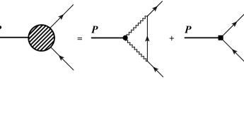
FIG. 1.: The lowest order contributions to the $P\to\ell^{+}\ell^{-}$ decay amplitude. The second graph denotes the contribution from the counterterm lagrangian of Eq. (6).

The corresponding expression for $s>4m_{\ell}^{2}$ is obtained by analytic continuation, using the usual $i\epsilon$ prescription. The loop diagram of Fig. 1 originates from the usual coupling of the light pseudoscalar mesons to a photon pair given by the well–known Wess–Zumino anomaly [4]. The divergence associated with this diagram has been renormalized within the ${\overline{\mbox{MS}}}$ minimal subtraction scheme of dimensional regularization. The logarithmic dependence on the renormalization scale $\mu$ displayed in the above expression is compensated by the scale dependence of the combination $\chi(\mu)$ of renormalized low–energy constants defined above. Let us stress here that, as shown explicitly in Eq. (3) and in contrast with the usual situation in the purely mesonic sector, this scale dependence is not suppressed in the large–$N_{C}$ limit, since it does not arise from meson loops. The evaluation of $\chi(\mu)$ will be the main subject of this paper.

It has recently been shown [5] that, when evaluated within the chiral $U(3)\otimes U(3)$ framework and in the $1/N_{C}$ expansion, the $|\Delta S|=1$ $K_{L}^{0}\to\ell^{+}\ell^{-}$ transitions can also be described by the expressions (2) and (3), with an effective constant $\chi_{K^{0}_{L}}$ containing an additional piece from the short–distance contributions [6]. Of course, a cast-iron understanding of these transitions is very important[7] as the evaluation of $\chi(\mu)$ could then have a potential impact on possible constraints on physics beyond the Standard Model. We comment on this issue at the end of the paper.

2. As a first step towards its subsequent evaluation we shall identify the coupling constant $\chi$ in terms of a QCD correlation function. For that purpose, consider the matrix element of the light quark isovector pseudoscalar density $P^{3}(x)\,=\,{1\over 2}({\bar{u}}i\gamma_{5}u-{\bar{d}}i\gamma_{5}d)(x)$ between leptonic states in the chiral limit. In the absence of weak interactions, and to lowest non–trivial order in the fine structure constant, this matrix element is given by the integral

$$\!\!\!\!<\ell^{-}(p^{\prime})\,|\,P^{3}(0)\,|\,\ell^{-}(p)>\qquad$$ (9)

$$\quad=e^{4}\int\frac{d^{4}q}{(2\pi)^{4}}\,\frac{{\bar{u}}(p^{\prime})\gamma^{\mu}[{\not\!p}^{\prime}-{\not\!q}+m_{\ell}]\gamma^{\nu}u(p)}{[(p^{\prime}-q)^{2}-m_{\ell}^{2}]q^{2}(p^{\prime}-p-q)^{2}}$$ (10)

$$\quad\times\,i\int d^{4}x\int d^{4}y\,e^{iq\cdot x}e^{i(p^{\prime}-p-q)\cdot y}$$ (11)

$$\quad\times<0\,|\,T\{j_{\mu}^{\mbox{{em}}}(x)j_{\nu}^{\mbox{{em}}}(y)P^{3}(0)\}\,|\,0>,$$ (12)

with $j_{\mu}^{\mbox{{em}}}={1\over 3}(2{\bar{u}}\gamma_{\mu}u-{\bar{d}}\gamma_{\mu}d-{\bar{s}}\gamma_{\mu}s)$. In the chiral limit, the QCD three–point correlator appearing in this expression is an order parameter of spontaneous chiral symmetry breaking. This ensures that it has a smooth behaviour at short distances. In particular, Bose symmetry and parity conservation of the strong interactions yield

$$\!\!\!\!\!\!\!\!\!\!\int d^{4}x\int d^{4}y\,e^{iq_{1}\cdot x}e^{iq_{2}\cdot y}$$ (13)

$$\times<0\,|\,T\{j_{\mu}^{\mbox{{em}}}(x)j_{\nu}^{\mbox{{em}}}(y)P^{3}(0)\}\,|\,0>$$ (14)

$$=\ \frac{2}{3}\,\epsilon_{\mu\nu\alpha\beta}q_{1}^{\alpha}q_{2}^{\beta}\,{\cal H}(q_{1}^{2},q_{2}^{2},(q_{1}+q_{2})^{2}),$$ (15)

with ${\cal H}(q_{1}^{2},q_{2}^{2},(q_{1}+q_{2})^{2})={\cal H}(q_{2}^{2},q_{1}^{2},(q_{1}+q_{2})^{2})$. For very large (euclidian) momenta, the leading short–distance behaviour of this correlation function is given by

$$\!\!\!\!\lim_{\lambda\to\infty}\,{\cal H}\big{(}(\lambda q_{1})^{2},(\lambda q_{2})^{2},(\lambda q_{1}+\lambda q_{2})^{2}\big{)}$$ (16)

$$=\ -\frac{1}{2\lambda^{4}}<{\bar{\psi}}\psi>\,\frac{q_{1}^{2}+q_{2}^{2}+(q_{1}+q_{2})^{2}}{q_{1}^{2}q_{2}^{2}(q_{1}+q_{2})^{2}}$$ (17)

$$\ +\,{\cal O}\bigg{(}\frac{\alpha_{s}}{\lambda^{4}},\frac{1}{\lambda^{6}}\bigg{)}.$$ (18)

Actually, what matters for the convergence of the integral in Eq. (12) is the leading short–distance singularity of the $T-$product of the two electromagnetic currents, which corresponds to

$$\!\!\!\!\lim_{\lambda\to\infty}\,{\cal H}\big{(}(\lambda q)^{2},(p^{\prime}-p-\lambda q)^{2},(p^{\prime}-p)^{2}\big{)}$$ (19)

$$=\ -\frac{1}{\lambda^{2}}<{\bar{\psi}}\psi>\,\frac{1}{q^{2}(p^{\prime}-p)^{2}}\,+\,{\cal O}\bigg{(}\frac{\alpha_{s}}{\lambda^{2}},\frac{1}{\lambda^{3}}\bigg{)},$$ (20)

and which implies that the loop integral in Eq. (12) is indeed convergent. The QCD corrections of order ${\cal O}(\alpha_{s})$ in Eqs. (18) and (20) will not be considered here. Let us however notice that since the pseudoscalar density $P^{3}(x)$ and the single–flavour $<{\bar{\psi}}\psi>$ condensate share the same anomalous dimension, the power–like fall–off displayed by Eqs. (18) and (20) is canonical, i.e. it is not modified by powers of logarithms of the momenta.

On the other hand, at very low momentum transfers, the same correlator can be computed within Chiral Perturbation Theory (ChPT). At lowest order, it is saturated by the pion–pole contribution, given by the anomalous coupling of a neutral pion, emitted by the pseudoscalar source $P^{3}(0)$, to the two electromagnetic currents, i.e.

$${\cal H}(0,0,(q_{1}+q_{2})^{2})\ =\ \,\frac{N_{C}}{8\pi^{2}}\,\frac{<{\bar{\psi}}\psi>}{F_{0}^{2}}\,\frac{1}{(q_{1}+q_{2})^{2}}\ +\cdots\ ,$$ (21)

where the ellipsis stands for higher orders in the low–momentum expansion and where $F_{0}$ denotes the pion decay constant in the chiral limit. The matrix element $<\ell^{-}(p^{\prime})\,|\,P^{3}(0)\,|\,\ell^{-}(p)>$ itself may also be evaluated in ChPT. At lowest order, it is given by the diagrams of Fig. 1, where the (off–shell) pion is now emitted by the pseudoscalar source $P^{3}(0)$. The result reads, with $t=(p^{\prime}-p)^{2}$,

$$\!\!\!\!\!\!\!\!<\ell^{-}(p^{\prime})\,|\,P^{3}(0)\,|\,\ell^{-}(p)>\big{|}_{\mbox{~{}{ChPT}}}$$ (22)

$$=\ -\frac{ie^{4}}{32\pi^{4}t}\,\frac{<{\bar{\psi}}\psi>}{F_{0}^{2}}\,m_{\ell}{\bar{u}}(p^{\prime})\gamma_{5}u(p)\,{\cal A}(t),$$ (23)

with the function ${\cal A}(t)$ defined in Eqs. (3) and (8). The contribution of the loop diagram of Fig. 1 is obtained upon replacing, in Eq. (12), the three–point QCD correlator by its lowest order chiral expression given in Eq. (21). The coupling constant $\chi(\mu)$ is thus given by the residue of the pole at $t=0$ of the matrix element $<\ell^{-}(p^{\prime})\,|\,P^{3}(0)\,|\,\ell^{-}(p)>$, after subtraction of the contribution of the two–photon loop, i.e.

$$\frac{\chi(\mu)}{32\pi^{4}}\,\frac{<{\bar{\psi}}\psi>}{F_{0}^{2}}\,m_{\ell}{\bar{u}}(p^{\prime})\gamma_{5}u(p)=\ -\frac{2i}{3}\,{\bar{u}}(p^{\prime})\gamma_{\lambda}\gamma_{5}u(p)$$ (24)

$$\times\lim_{(p^{\prime}-p)^{2}\to 0}\,\int\frac{d^{d}q}{(2\pi)^{d}}\frac{(p^{\prime}-p)^{2}}{[(p^{\prime}-q)^{2}-m_{\ell}^{2}]q^{2}(p^{\prime}-p-q)^{2}}$$ (25)

$$\times\,(p^{\prime}-p-2q)_{\alpha}\bigg{[}\,q^{\alpha}(p^{\prime}-p)^{\lambda}-\,(p^{\prime}-p)^{\alpha}q^{\lambda}\,\bigg{]}$$ (26)

$$\times\,\bigg{[}\,{\cal H}(q^{2},(p^{\prime}-p-q)^{2},(p^{\prime}-p)^{2})\,-\,{\cal H}(0,0,(p^{\prime}-p)^{2})\,\bigg{]}.$$ (27)

Since the integral occurring in the above expression diverges, we have regularized it by analytical continuation in the space–time dimension $d$. The coupling $\chi(\mu)$ on the left–hand side is then defined by the ${\overline{\mbox{MS}}}$ minimal subtraction prescription, as in Eq. (3). Keeping only the contributions that do not vanish as $(p^{\prime}-p)^{2}$ goes to zero, and neglecting terms of order ${\cal O}(m_{\ell}^{2}/\Lambda_{H}^{2})$, where $\Lambda_{H}\sim M_{\rho}$ is a typical hadronic scale for non–Goldstone mesonic states, we obtain a somewhat simpler expression,

$$\!\!\!\!\frac{\chi(\mu)}{32\pi^{4}}\,\frac{<{\bar{\psi}}\psi>}{F_{0}^{2}}=\ -\bigg{(}1\,-\,\frac{1}{d}\bigg{)}\,\int\frac{d^{d}q}{(2\pi)^{d}}\,\bigg{(}\frac{1}{q^{2}}\bigg{)}^{2}$$ (29)

$$\!\!\!\times\lim_{(p^{\prime}-p)^{2}\to 0}\,(p^{\prime}-p)^{2}\bigg{[}\,{\cal H}(q^{2},q^{2},(p^{\prime}-p)^{2})$$ (30)

$$\qquad\qquad\qquad\qquad\quad-\,{\cal H}(0,0,(p^{\prime}-p)^{2})\,\bigg{]}.$$ (31)

In order to perform this integral, one needs to extend the knowledge of the three–point correlation function ${\cal H}(q_{1}^{2},q_{2}^{2},(q_{1}+q_{2})^{2})$ in the chiral limit beyond its behaviour at energies very high, Eq. (18), or at energies very low, Eq. (21). Stated like that, in full generality, this represents a rather formidable task. As we shall next show, it is possible, however, following the examples discussed recently in Refs. [11, 12], to proceed further within the framework of the $1/N_{C}$–expansion in QCD [13].

3. In the limit where the number of colours $N_{C}$ becomes infinite, with $\alpha_{s}\times N_{C}$ staying finite, the QCD spectrum reduces to an infinite tower of zero–width mesonic resonances [14], and the leading large–$N_{C}$ contributions to the three–point correlator (15) are given by the tree–level exchanges of these resonances in the various channels, as shown in Fig. 2. This involves couplings of the resonances among themselves and to the external sources which, just like the masses of the resonances themselves, cannot be fixed in the absence of an explicit solution of QCD in the large–$N_{C}$ limit. In this limit, however, the analytical structure of the three–point function in Eq. (15) is very simple: the singularities in each channel consist of a succession of simple poles. Furthermore, the quantity appearing in Eq. (31) has the general structure

$$\!\!\!\!\lim_{(p^{\prime}-p)^{2}\to 0}\,(p^{\prime}-p)^{2}\,{\cal H}(q^{2},q^{2},(p^{\prime}-p)^{2})\ =\ -\frac{1}{2}\frac{<{\bar{\psi}}\psi>}{F_{0}^{2}}$$ (32)

$$\qquad\times\sum_{V}\,M_{V}^{2}\,\bigg{[}\,\frac{a_{V}}{(q^{2}-M_{V}^{2})}\,-\,\frac{b_{V}q^{2}}{(q^{2}-M_{V}^{2})^{2}}\,\bigg{]}\ ,$$ (33)

where a priori the sum extends over the infinite spectrum of vector resonances of QCD in the large–$N_{C}$ limit. Equation (33) follows from the fact that its left–hand side enjoys some additional properties: i) In the pseudoscalar channel, only the pion pole survives, while massive pseudoscalar resonances cannot contribute. ii) The momentum transfer in the two vector channels is the same. iii) Its high–energy behaviour is fixed by Eq. (20).

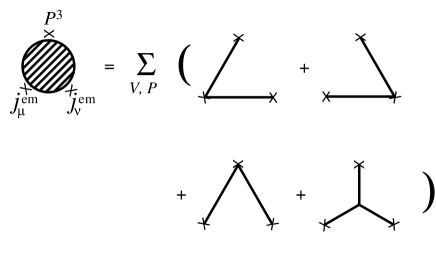
FIG. 2.: The contributions to the vector–vector–pseudoscalar three–point function in the large–$N_{C}$ limit of QCD. The sum extends over the infinite number of zero-width vector ($V$) and pseudoscalar ($P$) states.

Even though the constants $a_{V}$ and $b_{V}$ depend on the masses and couplings of the vector resonances in an unknown manner, they are however constrained by the two conditions

$$\sum_{V}\,a_{V}=\frac{N_{C}}{4\pi^{2}},\quad\sum_{V}\,(a_{V}\,-\,b_{V})\,M_{V}^{2}=2F_{0}^{2},$$ (34)

which follow from Eqs. (21) and (20), respectively. Notice that there are no contributions from the perturbative QCD continuum to these sums. Taking the first of these conditions (which, coming from the anomaly, has no ${\cal O}(\alpha_{s})$ corrections) into account, we obtain

$$\chi(\mu)=\frac{5N_{C}}{12}-2\pi^{2}\,\sum_{V}\,\bigg{[}\,a_{V}\ln\left(\frac{M_{V}^{2}}{\mu^{2}}\right)\,-\,b_{V}\,\bigg{]}.$$ (35)

This equation, together with the two conditions (34), constitutes the central result of our paper. This is as far as the large–$N_{C}$ limit allows us to go. Let us point out that the scale dependence of $\chi(\mu)$ is correctly reproduced by the expression (35), again as a consequence of the first condition in Eq. (34). However, in order to obtain a numerical estimate of $\chi(\mu)$ additional assumptions are needed.

4. In order to proceed further, we shall consider the Lowest Meson Dominance (LMD) approximation to the large–$N_{C}$ spectrum of vector meson resonances discussed in [15]. This approximation has been shown to reproduce very well the relevant low–energy constants of the ${\cal O}(p^{4})$ chiral Lagrangian [16] and the electromagnetic $\pi^{+}-\pi^{0}$ mass difference [11]. In our case, it corresponds to the assumption that the sums occurring in Eqs. (33) and (34) are saturated by the lowest lying vector meson octet. In the LMD approximation to large–$N_{C}$ QCD, the two conditions (34) completely pin down the two quantities $a_{V}$ and $b_{V}$ in terms of $F_{0}$ and of the mass $M_{V}$ of this lowest lying vector meson octet,

$$a_{V}^{\mbox{LMD}}=\frac{N_{C}}{4\pi^{2}}\quad\mbox{and}\quad b_{V}^{\mbox{LMD}}=\frac{N_{C}}{4\pi^{2}}\,-\,\frac{2F_{0}^{2}}{M_{V}^{2}}.$$ (36)

In fact, within the LMD approximation of large–$N_{C}$ QCD, it is easy to write down the expression for the correlation function ${\cal H}(q_{1}^{2},q_{2}^{2},(q_{1}+q_{2})^{2})$ which correctly interpolates between the high energy behaviour in Eq. (18) and the ChPT result in Eq. (21) [17]

$${\cal H}^{\mbox{LMD}}(q_{1}^{2},q_{2}^{2},(q_{1}+q_{2})^{2})\ =\ -\frac{1}{2}<{\bar{\psi}}\psi>$$ (37)

$$\times\frac{q_{1}^{2}+q_{2}^{2}+(q_{1}+q_{2})^{2}-M_{V}^{4}a_{V}^{\mbox{LMD}}/F_{0}^{2}}{(q_{1}^{2}-M_{V}^{2})(q_{2}^{2}-M_{V}^{2})(q_{1}+q_{2})^{2}}.$$ (38)

Notice that this expression also correctly reproduces the behaviour in Eq. (20). With the results of Eq. (36), and for $N_{C}$=3, it follows from Eq. (35) that

$$\chi^{\mbox{LMD}}(\mu)=\frac{11}{4}\,-\,\frac{3}{2}\ln\left(\frac{M_{V}^{2}}{\mu^{2}}\right)-4\pi^{2}\frac{F_{0}^{2}}{M_{V}^{2}}.$$ (39)

Numerically, using the physical values $F_{0}=92.4$ MeV and $M_{V}=M_{\rho}=770$ MeV, we obtain

$$\chi^{\mbox{LMD}}(\mu=M_{V})\ =\ 2.2\pm 0.9,$$ (40)

where we have allowed for a systematic theoretical error of 40%, as a rule of thumb estimate of the uncertainties attached to the large–$N_{C}$ and LMD approximations. The predicted ratios of branching ratios in Eq. (2) which follow from this result [10] are displayed in Table I. We conclude that, within errors, the LMD–approximation to large–$N_{C}$ QCD reproduces well the observed rates of pseudoscalar mesons decaying into lepton pairs.

5. At present, the most accurate experimental determination of the $K_{L}^{0}\to\mu^{+}\mu^{-}$ branching ratio [20] gives the result: $Br(K_{L}^{0}\to\mu^{+}\mu^{-})=(7.18\pm 0.17)\times 10^{-9}$. In the framework of the $1/N_{C}$ expansion and using the experimental branching ratio [2] $Br(K_{L}^{0}\to\gamma\gamma)=(5.92\pm 0.15)\times 10^{-4}$, this leads to a unique solution for an effective $\chi_{K_{L}^{0}}=5.17\pm 1.13$. Furthermore, following Ref. [5], $\chi_{K_{L}^{0}}=\chi-{\cal N}\ \delta\chi_{SD}$ where ${\cal N}=(3.6/g_{8}c_{\rm red})$ normalizes the $K_{L}^{0}\to\gamma\gamma$ amplitude. The coupling $g_{8}$ governs the $\Delta I=1/2$ rule, the constant $c_{\rm red}$ is defined in Ref. [5] and $\delta\chi_{SD}^{\mbox{\rm Standard}}=(+1.8\pm 0.6)$ is the short distance contribution in the Standard Model [6].

Therefore our understanding of the short distance contribution to this process completely hinges on our understanding of the long distance constant ${\cal N}$ and therefore of the $\Delta I=1/2$ rule in the $1/N_{C}$ expansion. Moreover, $c_{\rm red}$ is regretfully very unstable in the chiral and large-$N_{C}$ limits, a behaviour that surely points towards the need to have higher order corrections under control. For instance, for $M_{\pi}=0,M_{K}\not=0,N_{C}\rightarrow\infty$ one obtains $c_{\rm red}=0$, while for $M_{\pi}=M_{K}=0,N_{C}\rightarrow\infty$ (and the external $K_{L}^{0}$ off shell) one obtains $c_{\rm red}=-4/3$ instead. The analysis of Ref. [5] uses $c_{\rm red}\simeq+1$ and $g_{8}\simeq 3.6$, where these numbers are obtained phenomenologically by requiring agreement with the two-photon decay of $K_{L}^{0},\pi^{0},\eta$ and $\eta^{\prime}$ as well as $K\to 2\pi,3\pi$. Should we use these values of $c_{\rm red}$ and $g_{8}$ and Eq. (19) we would obtain $\chi_{K_{L}^{0}}=0.4\pm 1.1$, corresponding to a ratio $R(K_{L}^{0}\to\mu^{+}\mu^{-})=(2.24\pm 0.41)\times 10^{-5}$ which is $2.5\sigma$ above the experimental value $R(K_{L}^{0}\to\mu^{+}\mu^{-})=(1.21\pm 0.04)\times 10^{-5}$.

TABLE I.: The values for the ratios $R(P\to\ell^{+}\ell^{-})$ obtained within the LMD approximation to large–$N_{C}$ QCD and the comparison with available experimental results.

$R$	LMD	Experiment
$R(\pi^{0}\to e^{+}e^{-})\times 10^{8}$	$6.2\pm 0.3$	$7.13\pm 0.55$ [1]
$R(\eta\to\mu^{+}\mu^{-})\times 10^{5}$	$1.4\pm 0.2$	$1.48\pm 0.22$ [2]
$R(\eta\to e^{+}e^{-})\times 10^{8}$	$1.15\pm 0.05$	—

In view of these uncertainties we conclude that it does not seem to be possible, within our understanding of long–distance effects in the electroweak interactions, to argue that $K_{L}^{0}\to\mu^{+}\mu^{-}$ is, at present, a useful decay to constrain physics beyond the Standard Model.

We thank Ll. Ametller and A. Pich for discussions. Work supported in part by TMR, EC–Contract No. ERBFMRX–CT980169. The work of S.P. is also supported by AEN98-1093.

REFERENCES

[1]
A. Alavi-Harati et al., hep-exp/9903007 and references therein.
[2]
C. Caso et al., Review of Particle Physics, Eur. Phys. J. C3
1 (1998), and references therein.
[3]
M.J. Savage, M. Luke and M.B. Wise, Phys. Lett.B291, 481
(1992).
[4]
J. Wess and B. Zumino, Phys. Lett. B37 95 (1971).
[5]
D. Gómez Dumm and A. Pich, Phys. Rev. Lett. 80, 4633 (1998).
[6]
G. Buchalla and A.J. Buras, Nucl. Phys. B412, 106 (1994);
A.J. Buras and R. Fleischer, in Heavy Flavours II, edited
by A.J. Buras and M. Linder, hep-ph/9704376.
[7]
We refer the reader to Ref. [5] for further details. See
also Refs. [8] and [9] for an alternative approach.
[8]
G. D’Ambrosio, G. Isidori and J. Portolés, Phys. Lett. B423,
385 (1998).
[9]
G. Valencia, Nucl. Phys. B517, 339 (1998).
[10]
In the case of the
decay into a muon pair,
corrections lower the result of
Eq. (40) by about 7%, and are taken into account in the
numerical values of Table I.
[11]
M. Knecht, S. Peris and E. de Rafael, Phys. Lett. B443,
255 (1998).
[12]
M. Knecht, S. Peris and E. de Rafael, Phys. Lett. B457,
227 (1999).
[15]
S. Peris, M. Perrottet and E. de Rafael, JHEP 05, 011
(1998). See also, M. Golterman and S. Peris, hep-ph/9908252.
[16]
J. Gasser and H. Leutwyler, Nucl. Phys. B250, 465 (1984).
[17]
A similar analysis for the
vector–vector–scalar and
vector–axial–pseudoscalar three–point
functions can be found in Refs. [18] and [19],
respectively.
[18]
B. Moussallam and J. Stern, in Two - Photon Physics: From
DAPHNE to LEP 200 and Beyond, edited by F. Kapusta and J.J. Parisi,
World Scientific (1994), and hep-ph/9404353.
[19]
B. Moussallam, Nucl. Phys. B504, 381 (1997).
[20]
D. Ambrose et al., reported at the KAON’99 Workshop,
Chicago, June 1999, (to be published).