Bosonic Quartic Couplings at LEP2

G. Bélanger1, F. Boudjema1, Y. Kurihara2, D. Perret-Gallix3, A. Semenov4

1. Laboratoire de Physique Théorique LAPTH

Chemin de Bellevue, B.P. 110, F-74941 Annecy-le-Vieux, Cedex, France.

2. High Energy Accelerator Research Organisation, KEK,

Tsukuba, Ibaraki 305-801, Japan.

3. LAPP

Chemin de Bellevue, B.P. 110, F-74941 Annecy-le-Vieux, Cedex, France.

4. Joint Institute for Nuclear Research, JINR,

141980 Dubna, Russia.

Abstract

We list the set of ${\cal{C}}\;$and ${\cal{P}}\;$conserving anomalous quartic vector bosons self-couplings which can be tested at LEP2 through triple vector boson production. We show how this set can be embedded in manifestly $SU(2)\times U(1)$ gauge invariant operators exhibiting an $SU(2)_{c}$ global symmetry. We derive bounds on these various couplings and show the most relevant distributions that can enhance their contribution. We also find that an $e^{+}e^{-}$ collider running at $500$ GeV can improve the LEP2 limits by as much as three-orders of magnitude.

KEK-CP-087

LAPTH-744/99

1 Photonic Quartic Couplings

LEP has now crossed the threshold for Z pair production and therefore experiments can now study triple boson production like $e^{+}e^{-}\;\rightarrow W^{+}W^{-}\gamma,ZZ\gamma$, beside $e^{+}e^{-}\;\rightarrow\gamma\gamma\gamma,\gamma\gamma Z$ which may be studied at lower energies. These processes have the potential to study new quartic photonic couplings, photonic in the sense that at least one of the vector bosons is a photon. One should refer to these quartic couplings as genuine quartic couplings [1, 2, 3] contrary to quartic couplings that may emerge from an operator that induces for instance both a tri-linear $WW\gamma$ coupling as well as a possible $WW\gamma\gamma$, as required by gauge invariance. The latter (non-genuine) couplings can therefore be investigated much more efficiently through their tri-linear counterpart in, for instance, $e^{+}e^{-}\;\rightarrow W^{+}W^{-}$. An example of such a coupling is the much studied operator described by $\lambda_{\gamma}$ in the by now classic classification [4] , $\lambda_{\gamma}$ is sometimes referred to as the anomalous quadrupole moment of the $W$. From this perspective genuine quartic couplings can only be studied in triple vector boson production or through boson-boson fusion, the latter becoming a more efficient means at TeV energies [3].

Let us note that quartic neutral couplings, $4-\gamma\;,\;Z-3\gamma$, contributing to $e^{+}e^{-}\;\rightarrow 3\gamma$ have already been studied in [2] and could be explored for energies below those presently available. Since these quartic couplings involve at least three photons, electromagnetic gauge invariance alone allows these couplings only if they emerge from dimension-eight (or higher) operators. On the other hand, anomalous couplings such as $WW\gamma\gamma$ or $WWZ\gamma$ that contribute to $e^{+}e^{-}\rightarrow W^{+}W^{-}\gamma\;$may be associated to dim-6 operators and are hence a more likely signal of a possible residual effects of New Physics. As a matter of fact $WW\gamma\gamma$ and $WWZ\gamma$ are present in the ${\cal{S}}{\cal{M}}\;$at tree-level and as a consequence these types of couplings are more important to study. These quartic photonic couplings were first introduced in [1] in view of studying their effects on $\gamma\gamma\rightarrow W^{+}W^{-}\;$in the laser mode of the Linear Collider. They were derived by only appealing to electromagnetic gauge invariance and $SU(2)_{c}$ custodial symmetry. The phenomenology of these couplings has since then been studied in the next linear collider both in the $e^{+}e^{-}\;$[3, 5], $\gamma\gamma$ [1] and $e\gamma$ [6] modes. Very recently these couplings have been re-investigated for LEP2 energies [7]. Unfortunately, as we will show, when studying the effect of genuine quartic couplings in $e^{+}e^{-}\rightarrow W^{+}W^{-}\gamma\;$and $e^{+}e^{-}\;\rightarrow Z\gamma\gamma$, one needs to consider a larger set of structures than the two that have been written down for $\gamma\gamma\rightarrow W^{+}W^{-}\;$. The aim of this paper is to generalize the study we performed in [1, 3] and to review and clarify some of the issues related to the photonic quartic couplings.

The plan of the paper is as follows. In the next section, we start by first listing the leading quartic operators that contribute to $e^{+}e^{-}\;\rightarrow W^{+}W^{-}\gamma$ (and $Z\gamma\gamma$). In writing down this list we will only appeal to explicit $U(1)_{\rm em}$ gauge invariance as well as ${\cal{C}}\;$and ${\cal{P}}\;$conservation. In a sense these structures constitute the quartic counterpart to the tri-linear classification in [4]. In passing we will point out that a third “photonic” quartic coupling that has been entertained [6, 7] in the literature does in fact violate ${\cal{C}}{\cal{P}}\;$. We will then show how the different structures can be embedded within $SU(2)\times U(1)$ operators which we require also to exhibit the $SU(2)_{c}$ global custodial symmetry which leads to $\rho=1$ in the limit of vanishing hypercharge coupling. This can be done either in the usual approach by exploiting the covariant derivative on the Goldstone-Higgs field (for notations and conventions refer to [8, 9]) or in the non-linear chiral approach of symmetry breaking (see [8, 10]). The explicitly $SU(2)\times U(1)$ approach together with the $SU(2)$ global symmetry will allow to relate some $WW\gamma\gamma$ and $ZZ\gamma\gamma$ structures, for example. In section 3 we turn to the analysis of these quartic couplings in $e^{+}e^{-}\rightarrow W^{+}W^{-}\gamma\;$and $e^{+}e^{-}\;\rightarrow Z\gamma\gamma$. We will derive the limits one may hope to extract and show the distributions which are most sensitive to these couplings. The case of the ${\cal{C}}{\cal{P}}\;$violating operator is relegated to an Appendix.

2 Structures which contribute to $e^{+}e^{-}\rightarrow W^{+}W^{-}\gamma\;$, $Z\gamma\gamma$ and $ZZ\gamma$

For LEP2, the processes of interest, and the lowest-dimension anomalous quartic couplings they are sensitive to, are

• $e^{+}e^{-}\;\rightarrow W^{+}W^{-}\gamma\;\;\;\;\;\longrightarrow{\rm quartic:}\;\;WW\gamma\gamma,WWZ\gamma$

• $e^{+}e^{-}\;\rightarrow Z\gamma\gamma\;\;\;\;\;\longrightarrow{\rm quartic}\;\;ZZ\gamma\gamma$

• $e^{+}e^{-}\;\rightarrow ZZ\gamma\;\;\;\;\;\longrightarrow{\rm quartic}\;\;ZZZ\gamma,ZZ\gamma\gamma$

Due to phase space the latter process is marginal at LEP2. Note that for $Z\gamma\gamma$ production only one coupling is checked, $ZZ\gamma\gamma$, if one restricts oneself to the lowest dimension operators, otherwise a $Z3\gamma$ which is of highest dimension may also contribute. Already at LEP2, one may also exploit $e^{+}e^{-}\;\rightarrow\nu\bar{\nu}\gamma\gamma$ as a testing ground for the quartic coupling $WW\gamma\gamma$, as suggested in [7, 11].

We start by listing all those genuine quartic bosonic operators that contribute to the latter processes and which are of lowest possible dimension, as it turns out, dim-6. We first only require electromagnetic gauge invariance together with ${\cal{C}}\;$and ${\cal{P}}\;$symmetry. At this stage the $WW\gamma\gamma$, $WWZ\gamma$ or $ZZ\gamma\gamma$ couplings, for example, are not related. Each photon requires the use of the electromagnetic tensor $F_{\mu\nu}=\partial_{\mu}A_{\nu}-\partial_{\nu}A_{\mu}$. As we have shown elsewhere [1], there can be only two basic Lorentz structures for the lowest dimension $WW\gamma\gamma$ operators. These map into the parameters $a_{0}$ and $a_{c}$ first introduced in [1, 3]. Hence the two $WW\gamma\gamma$ Lorentz structures are:

$${{\cal W}}_{0}^{\gamma} = -\frac{e^{2}g^{2}}{2\Lambda^{2}}\;F_{\mu\nu}F^{\mu\nu}W^{+\alpha}W^{-}_{\alpha}$$

$${{\cal W}}_{c}^{\gamma} = -\frac{e^{2}g^{2}}{4\Lambda^{2}}\;F_{\mu\nu}F^{\mu\alpha}\left(W^{+\nu}W^{-}_{\alpha}\;+\;W^{-\nu}W^{+}_{\alpha}\right)$$ (2.1)

where $e$ is the electromagnetic coupling, $g=e/\sin\theta_{W}=e/s_{W}$ and $\Lambda$ a mass scale characterizing the New Physics.

For $W^{+}W^{-}Z\gamma$, it is also easy to see that one can have a maximum of $5$ independent structures. With $g_{Z}=e/s_{W}c_{W}$ and $V_{\mu\nu}=\partial_{\mu}V_{\nu}-\partial_{\nu}V_{\mu}$ where $V=W^{\pm},Z$, we have

$${{\cal W}}_{0}^{Z} = -\frac{e^{2}g^{2}}{\Lambda^{2}}F_{\mu\nu}Z^{\mu\nu}W^{+\alpha}W^{-}_{\alpha}$$

$${{\cal W}}_{c}^{Z} = -\frac{e^{2}g^{2}}{2\Lambda^{2}}F_{\mu\nu}Z^{\mu\alpha}\left(W^{+\nu}W^{-}_{\alpha}\;+\;W^{-\nu}W^{+}_{\alpha}\right)$$

$${{\cal W}}_{1}^{Z} = -\frac{eg_{Z}g^{2}}{2\Lambda^{2}}\;F^{\mu\nu}\left(W^{+}_{\mu\nu}W^{-}_{\alpha}Z^{\alpha}\;+\;W^{-}_{\mu\nu}W^{+}_{\alpha}Z^{\alpha}\right)$$

$${{\cal W}}_{2}^{Z} = -\frac{eg_{Z}g^{2}}{2\Lambda^{2}}\;F^{\mu\nu}\left(W^{+}_{\mu\alpha}W^{-\alpha}Z_{\nu}\;+\;W^{-}_{\mu\alpha}W^{+\alpha}Z_{\nu}\right)$$

$${{\cal W}}_{3}^{Z} = -\frac{eg_{Z}g^{2}}{2\Lambda^{2}}\;F^{\mu\nu}\left(W^{+}_{\mu\alpha}W^{-}_{\nu}Z^{\alpha}\;+\;W^{-}_{\mu\alpha}W^{+}_{\nu}Z^{\alpha}\right)$$

Note that instead of the use of the field tensor, $V_{\mu\nu}$, for one of the massive vector boson in Eq. 2, we could have used instead a simple derivative, $\partial_{\mu}V_{\nu}$. However it is easy to show that using the derivative only maps into one/or a combination of the above $7$ operators, if one requires the photon from Eq. 2 to be on-shell like in the process of interest, $e^{+}e^{-}\rightarrow W^{+}W^{-}\gamma\;$. Therefore, all in all, there are 7 ${\cal{C}}\;$and ${\cal{P}}\;$conserving Lorentz structures which at leading order contribute to $e^{+}e^{-}\rightarrow W^{+}W^{-}\gamma\;$. Note that at high enough energy one may differentiate, in $e^{+}e^{-}\rightarrow W^{+}W^{-}\gamma\;$, between the quartic couplings of type ${{\cal W}}_{0,c}$ and those of the type ${{\cal W}}_{1,2,3}^{Z}$ if one is able to reconstruct the final polarisation of the $W$’s. Indeed both $W$’s in the former are preferentially longitudinal whereas in the latter, one is transverse and the other longitudinal, this is because in the latter the operators involve at least a field strength to describe a $W$.

It is straightforward to “convert” the above operators to genuine quartic couplings for $ZZ\gamma\gamma$ and $ZZZ\gamma$ which contribute to $e^{+}e^{-}\;\rightarrow Z\gamma\gamma$ and $e^{+}e^{-}\;\rightarrow ZZ\gamma$. One counts two independent operators for $ZZ\gamma\gamma$

$${{\cal Z}}_{0}^{\gamma} = -\frac{e^{2}g_{Z}^{2}}{4\Lambda^{2}}\;F_{\mu\nu}F^{\mu\nu}Z^{\alpha}Z_{\alpha}$$

$${{\cal Z}}_{c}^{\gamma} = -\frac{e^{2}g_{Z}^{2}}{4\Lambda^{2}}\;F_{\mu\nu}F^{\mu\alpha}Z^{\nu}Z_{\alpha}$$ (2.3)

and two for $ZZZ\gamma$

$${{\cal Z}}_{0}^{Z} = -\frac{e^{2}g_{Z}^{2}}{2\Lambda^{2}}\;F_{\mu\nu}Z^{\mu\nu}Z^{\alpha}Z_{\alpha}$$

$${{\cal Z}}_{c}^{Z} = -\frac{e^{2}g_{Z}^{2}}{2\Lambda^{2}}\;F_{\mu\nu}Z^{\mu\alpha}Z^{\nu}Z_{\alpha}$$ (2.4)

2.1 Feynman Rules

The Feynman rules for the above operators are easy to derive. It is worth noticing that all the above operators can be expressed in terms of very few Lorentz structures. We define

$${{\cal P}}_{0}(A(k_{1},\mu);N(k_{2},\nu);V_{\alpha}\;;V_{\beta})=\frac{ie^{2}g^{2}}{\Lambda^{2}}\;\;2\;g_{\alpha\beta}(g_{\mu\nu}k_{1}.k_{2}-k_{1\nu}k_{2\mu})$$ (2.5)

$k_{i}$ stand for the momentum of the particle and $\{\mu\;\nu\;\alpha\;\beta\}$ are the Lorentz indices.

$${{\cal P}}_{c}(A(k_{1},\mu);N(k_{2},\nu);V_{\alpha};V_{\beta})=\frac{ie^{2}g^{2}}{2\Lambda^{2}}\;\;$$

$$\left((g_{\mu\alpha}g_{\nu\beta}+g_{\nu\alpha}g_{\mu\beta})k_{1}.k_{2}\;+\;g_{\mu\nu}(k_{2\beta}k_{1\alpha}+k_{1\beta}k_{2\alpha})\right.$$

$$-\left.k_{2\mu}k_{1\alpha}g_{\nu\beta}\;-\;k_{2\beta}k_{1\nu}g_{\mu\alpha}\;-\;k_{2\alpha}k_{1\nu}g_{\mu\beta}\;-\;k_{2\mu}k_{1\beta}g_{\nu\alpha}\right)$$ (2.6)

For the $WWZ\gamma$ with no $WW\gamma\gamma$ equivalent, the last three structures in Eq. 2, three more structures are needed

$${{\cal P}}_{1}(A(k_{1},\mu);Z(k_{2},\nu);W^{+}(k_{+},\alpha);W^{-}(k_{-},\beta))=\frac{ieg_{Z}g^{2}}{\Lambda^{2}}\;\;$$

$$\left((k_{1}.k_{+}g_{\mu\alpha}-k_{+\mu}k_{1\alpha})g_{\nu\beta}\;+\;(k_{1}.k_{-}g_{\mu\beta}-k_{-\mu}k_{1\beta})g_{\nu\alpha}\right)$$ (2.7)

$${{\cal P}}_{2}(A(k_{1},\mu);Z(k_{2},\nu);W^{+}(k_{+},\alpha);W^{-}(k_{-},\beta))=\frac{ieg_{Z}g^{2}}{2\Lambda^{2}}\;\;$$

$$\left((k_{1}.k_{+}+k_{1}.k_{-})g_{\mu\nu}g_{\alpha\beta}\;-\;(k_{1\alpha}k_{+\beta}+k_{1\beta}k_{-\alpha})g_{\mu\nu}\right.$$

$$-\left.(k_{+\mu}+k_{-\mu})k_{1\nu}g_{\alpha\beta}\;+\;(k_{+\beta}g_{\mu\alpha}+k_{-\alpha}g_{\mu\beta})k_{1\nu}\right)$$ (2.8)

$${{\cal P}}_{3}(A(k_{1},\mu);Z(k_{2},\nu);W^{+}(k_{+},\alpha);W^{-}(k_{-},\beta))=\frac{ieg_{Z}g^{2}}{2\Lambda^{2}}\;\;$$

$$\left(k_{1}.k_{+}g_{\mu\beta}g_{\nu\alpha}\;+\;k_{1}.k_{-}g_{\mu\alpha}g_{\nu\beta}\;+\;(k_{+\nu}-k_{-\nu})k_{1\beta}g_{\mu\alpha}\right.$$

$$-\left.(k_{+\nu}-k_{-\nu})k_{1\alpha}g_{\mu\beta}\;-\;k_{+\mu}k_{1\beta}g_{\nu\alpha}\;-\;k_{-\mu}k_{1\alpha}g_{\nu\beta}\right)$$ (2.9)

For the couplings of four neutral bosons, it is useful to introduce

$${{\cal P}}_{0,c}^{Z}={{\cal P}}_{0,c}(g\rightarrow g_{Z})$$ (2.10)

then taking all particles to be incoming, the Feynman rules are

$${{\cal W}}_{0,c}^{\gamma} \rightarrow {{\cal P}}_{0,c}(A(k_{1},\mu);A(k_{2},\nu);W^{+}(\alpha);W^{-}(\beta))$$

$${{\cal W}}_{0,c}^{Z} \rightarrow {{\cal P}}_{0,c}(A(k_{1},\mu);Z(k_{2},\nu);W^{+}(\alpha);W^{-}(\beta))$$

$${{\cal W}}_{1,2,3}^{Z} \rightarrow {{\cal P}}_{1,2,3}(A(k_{1},\mu);Z(k_{2},\nu);W^{+}(k_{+}\alpha);W^{-}(k_{-}\beta))$$

$${{\cal Z}}_{0,c}^{\gamma} \rightarrow {{\cal P}}_{0,c}^{Z}(A(k_{1},\mu);A(k_{2},\nu);Z(\alpha);Z(\beta))$$

$${{\cal Z}}_{0,c}^{Z} \rightarrow {{\cal P}}_{0,c}^{Z}(A(k,\mu);Z(k_{1},\nu);Z(k_{2}\rho);Z(k_{3}\lambda))\;+\;\left((k_{1},\nu)\leftrightarrow(k_{2},\rho)\right)\;+\;\left((k_{1},\nu)\leftrightarrow(k_{3},\lambda)\right)$$

2.2 Embedding in gauge invariant $SU(2)_{c}$ symmetric operators

All the above operators can be embedded in manifestly $SU(2)\times U(1)$ gauge invariant and $SU(2)_{c}$ symmetric operators, which are then ${\cal{C}}\;$and ${\cal{P}}\;$conserving. The construction has been explained at some length in [8]. For these kind of quartic operators it is more appropriate to use the chiral Lagrangian approach, which assumes no Higgs. The leading order operators in the energy expansion reproduce the “Higgsless” standard model. Introducing our notations, as concerns the purely bosonic sector, the SU(2) kinetic term that gives the standard tree-level gauge self-couplings is

$${{\cal L}}_{{\rm Gauge}}=-\frac{1}{2}\left[{\rm Tr}({\mbox{\boldmath$W$}}_{\mu\nu}{\mbox{\boldmath$W$}}^{\mu\nu})+{\rm Tr}({\mbox{\boldmath$B$}}_{\mu\nu}{\mbox{\boldmath$B$}}^{\mu\nu})\right]$$ (2.12)

where the $SU(2)$ gauge fields are ${\mbox{\boldmath$W$}}_{\mu}=W^{i}_{\mu}\tau^{i}$, while the hypercharge field is denoted by ${\mbox{\boldmath$B$}}_{\mu}=\tau_{3}B_{\mu}$. The normalisation for the Pauli matrices is ${\rm Tr}(\tau^{i}\tau^{j})=2\delta^{ij}$. We define the field strength as, ${\mbox{\boldmath$W$}}_{\mu\nu}$

$${\mbox{\boldmath$W$}}_{\mu\nu} = \frac{1}{2}\left(\partial_{\mu}{\mbox{\boldmath$W$}}_{\nu}-\partial_{\nu}{\mbox{\boldmath$W$}}_{\mu}+\frac{i}{2}g[{\mbox{\boldmath$W$}}_{\mu},{\mbox{\boldmath$W$}}_{\nu}]\right)$$ (2.13)

$$= \frac{\tau^{i}}{2}\left(\partial_{\mu}W^{i}_{\nu}-\partial_{\nu}W^{i}_{\mu}-g\epsilon^{ijk}W_{\mu}^{j}W_{\nu}^{k}\right)$$

The Goldstone bosons, $\omega^{i}$, within the built-in SU(2) symmetry are assembled in a matrix $\Sigma$

$$\Sigma=exp(\frac{i\omega^{i}\tau^{i}}{v})\;\;;v=246~{}GeV\;\;\;\mbox{ and}\;\;{{\cal D}}_{\mu}\Sigma=\partial_{\mu}\Sigma+\frac{i}{2}\left(g{\mbox{\boldmath$W$}}_{\mu}\Sigma-g^{\prime}B_{\mu}\Sigma\tau_{3}\right)\;;\;g^{\prime}=e/c_{W}$$

This leads to the gauge invariant mass term for the $W$ and $Z$

$${{\cal L}}_{M}=\frac{v^{2}}{4}{\rm Tr}({{\cal D}}^{\mu}\Sigma^{\dagger}{{\cal D}}_{\mu}\Sigma)\equiv-\frac{v^{2}}{4}{\rm Tr}\left({\mbox{\boldmath$V$}}_{\mu}{\mbox{\boldmath$V$}}^{\mu}\right)\;\;\;\;;\;\;{\mbox{\boldmath$V$}}_{\mu}=\left({{\cal D}}_{\mu}\Sigma\right)\Sigma^{\dagger}\;\;;\;\;M_{W}=\frac{gv}{2}$$ (2.15)

Incidentally, in the unitary gauge, ${\mbox{\boldmath$V$}}_{\mu}$ corresponds to the triplet of the massive gauge bosons $W^{\pm},Z$. Note also that at the next-to-leading order in the chiral Lagrangian approach there are genuine quartic couplings, however they only involve the massive vector bosons, $WWWW,WWZZ,ZZZZ$. These quartic couplings can not, unfortunately, be studied at LEP2. They are described, in the $SU(2)_{c}$ limit,

$${{\cal L}}_{NLO}=\frac{L_{1}}{16\pi^{2}}\left({\rm Tr}({\mbox{\boldmath$V$}}_{\mu}{\mbox{\boldmath$V$}}^{\mu})\right)^{2}+\frac{L_{2}}{16\pi^{2}}\left({\rm Tr}({\mbox{\boldmath$V$}}^{\mu}{\mbox{\boldmath$V$}}_{\nu})\right)^{2}$$ (2.16)

Photonic quartic operators appear first as next-to-next-to-leading operators. Even by requiring $SU(2)_{c}$, ${\cal{C}}\;$and ${\cal{P}}\;$conservation there are quite a few quartic photonic operators. We list them below and show the contribution of each to the quartic Lorentz structures of interest, described earlier in Eqs. 2- 2. The $\dots$ represent possible $4W,4Z,WWZZ$ as well as Goldstones vertices. The $k_{i}^{j}$ parameterise the strength of the anomalous coupling. By exploiting properties of the trace of unitary $2\times 2$ matrices, other possible combinations of operators can be expressed as combinations of the operators given below.

$$\frac{k_{0}^{w}}{\Lambda^{2}}\;g^{2}\;{\rm Tr}({\mbox{\boldmath$W$}}_{\mu\nu}{\mbox{\boldmath$W$}}^{\mu\nu}){\rm Tr}({\mbox{\boldmath$V$}}^{\alpha}{\mbox{\boldmath$V$}}_{\alpha}) \rightarrow k_{0}^{w}\left(\right.\;{{\cal Z}}_{0}^{\gamma}\;+\;\frac{c_{W}}{s_{W}}{{\cal Z}}_{0}^{Z}\;+\;{{\cal W}}_{0}^{\gamma}\;+\;\frac{c_{W}}{s_{W}}{{\cal W}}_{0}^{Z}\;+\;\dots$$

$$\frac{k_{c}^{w}}{\Lambda^{2}}\;g^{2}\;{\rm Tr}({\mbox{\boldmath$W$}}_{\mu\nu}{\mbox{\boldmath$W$}}^{\mu\alpha}){\rm Tr}({\mbox{\boldmath$V$}}^{\nu}{\mbox{\boldmath$V$}}_{\alpha}) \rightarrow k_{c}^{w}\left(\right.{{\cal Z}}_{c}^{\gamma}\;+\;\frac{c_{W}}{s_{W}}{{\cal Z}}_{c}^{Z}\;+\;{{\cal W}}_{c}^{\gamma}\;+\;\frac{c_{W}}{s_{W}}{{\cal W}}_{c}^{Z}\;+\;\dots$$

$$\frac{k_{1}^{w}}{\Lambda^{2}}\;g^{2}\;{\rm Tr}({\mbox{\boldmath$W$}}_{\mu\nu}{\mbox{\boldmath$V$}}^{\alpha}){\rm Tr}({\mbox{\boldmath$W$}}^{\mu\nu}{\mbox{\boldmath$V$}}_{\alpha}) \rightarrow k_{1}^{w}\left(\right.{{\cal Z}}_{0}^{\gamma}\;+\;\frac{c_{W}}{s_{W}}{{\cal Z}}_{0}^{Z}\;+\;{{\cal W}}_{1}^{Z}\;+\;\dots$$ (2.19)

$$\frac{k_{2}^{w}}{\Lambda^{2}}\;g^{2}\;{\rm Tr}({\mbox{\boldmath$W$}}_{\mu\nu}{\mbox{\boldmath$V$}}^{\nu}){\rm Tr}({\mbox{\boldmath$W$}}^{\mu\alpha}{\mbox{\boldmath$V$}}_{\alpha}) \rightarrow k_{2}^{w}\left(\right.{{\cal Z}}_{c}^{\gamma}\;+\;\frac{c_{W}}{s_{W}}{{\cal Z}}_{c}^{Z}\;+\;{{\cal W}}_{2}^{Z}\;+\;\dots$$ (2.20)

$$\frac{k_{3}^{w}}{\Lambda^{2}}\;g^{2}\;{\rm Tr}({\mbox{\boldmath$W$}}_{\mu\nu}{\mbox{\boldmath$V$}}_{\alpha}){\rm Tr}({\mbox{\boldmath$W$}}^{\mu\alpha}{\mbox{\boldmath$V$}}^{\nu}) \rightarrow k_{3}^{w}\left(\right.{{\cal Z}}_{c}^{\gamma}\;+\;\frac{c_{W}}{s_{W}}{{\cal Z}}_{c}^{Z}\;+\;{{\cal W}}_{3}^{Z}\;+\;\dots$$ (2.21)

$$\frac{k_{0}^{b}}{\Lambda^{2}}\;g^{\prime 2}{\rm Tr}({\mbox{\boldmath$B$}}_{\mu\nu}{\mbox{\boldmath$B$}}^{\mu\nu}){\rm Tr}({\mbox{\boldmath$V$}}^{\alpha}{\mbox{\boldmath$V$}}_{\alpha}) \rightarrow k_{0}^{b}\left(\right.{{\cal Z}}_{0}^{\gamma}\;-\;\frac{s_{W}}{c_{W}}{{\cal Z}}_{0}^{Z}\;+\;{{\cal W}}_{0}^{\gamma}\;-\;\frac{s_{W}}{c_{W}}{{\cal W}}_{0}^{Z}\;+\;\dots$$

$$\frac{k_{c}^{b}}{\Lambda^{2}}\;g^{\prime 2}{\rm Tr}({\mbox{\boldmath$B$}}_{\mu\nu}{\mbox{\boldmath$B$}}^{\mu\alpha}){\rm Tr}({\mbox{\boldmath$V$}}^{\nu}{\mbox{\boldmath$V$}}_{\alpha}) \rightarrow k_{c}^{b}\left(\right.{{\cal Z}}_{c}^{\gamma}\;-\;\frac{s_{W}}{c_{W}}{{\cal Z}}_{c}^{Z}\;+\;{{\cal W}}_{c}^{\gamma}\;-\;\frac{s_{W}}{c_{W}}{{\cal W}}_{c}^{Z}\;+\;\dots$$

$$\frac{k_{1}^{b}}{\Lambda^{2}}\;g^{\prime 2}{\rm Tr}({\mbox{\boldmath$B$}}_{\mu\nu}{\mbox{\boldmath$V$}}^{\alpha}){\rm Tr}({\mbox{\boldmath$B$}}^{\mu\nu}{\mbox{\boldmath$V$}}_{\alpha}) \rightarrow k_{1}^{b}\left(\right.{{\cal Z}}_{0}^{\gamma}\;-\;\frac{s_{W}}{c_{W}}{{\cal Z}}_{0}^{Z}\;+\;\dots$$ (2.24)

$$\frac{k_{2}^{b}}{\Lambda^{2}}\;g^{\prime 2}{\rm Tr}({\mbox{\boldmath$B$}}_{\mu\nu}{\mbox{\boldmath$V$}}^{\nu}){\rm Tr}({\mbox{\boldmath$B$}}^{\mu\alpha}{\mbox{\boldmath$V$}}_{\alpha}) \rightarrow k_{2}^{b}\left(\right.{{\cal Z}}_{c}^{\gamma}\;-\;\frac{s_{W}}{c_{W}}{{\cal Z}}_{c}^{Z}\;+\;\dots$$ (2.25)

and

$$\frac{k_{0}^{m}}{\Lambda^{2}}\;gg^{\prime}{\rm Tr}({\mbox{\boldmath$W$}}_{\mu\nu}{\mbox{\boldmath$B$}}^{\mu\nu}){\rm Tr}({\mbox{\boldmath$V$}}^{\alpha}{\mbox{\boldmath$V$}}_{\alpha}) \rightarrow k_{0}^{m}\left(\right.{{\cal Z}}_{0}^{\gamma}\;+\;c_{ZW}{{\cal Z}}_{0}^{Z}\;+\;{{\cal W}}_{0}^{\gamma}\;+\;c_{ZW}{{\cal W}}_{0}^{Z}\;+\;\dots$$

$$\frac{k_{c}^{m}}{\Lambda^{2}}\;gg^{\prime}{\rm Tr}({\mbox{\boldmath$W$}}_{\mu\nu}{\mbox{\boldmath$B$}}^{\mu\alpha}){\rm Tr}({\mbox{\boldmath$V$}}^{\nu}{\mbox{\boldmath$V$}}_{\alpha}) \rightarrow k_{c}^{m}\left(\right.{{\cal Z}}_{c}^{\gamma}\;+\;c_{ZW}{{\cal Z}}_{c}^{Z}\;+\;{{\cal W}}_{c}^{\gamma}\;+\;c_{ZW}{{\cal W}}_{c}^{Z}\;+\;\dots$$

$$\frac{k_{1}^{m}}{\Lambda^{2}}\;gg^{\prime}{\rm Tr}({\mbox{\boldmath$W$}}_{\mu\nu}{\mbox{\boldmath$V$}}^{\alpha}){\rm Tr}({\mbox{\boldmath$B$}}^{\mu\nu}{\mbox{\boldmath$V$}}_{\alpha}) \rightarrow k_{1}^{m}\left(\right.{{\cal Z}}_{0}^{\gamma}\;+\;c_{ZW}{{\cal Z}}_{0}^{Z}\;+\;\frac{1}{2}{{\cal W}}_{1}^{Z}\;+\;\dots$$ (2.28)

$$\frac{k_{2}^{m}}{\Lambda^{2}}\;gg^{\prime}{\rm Tr}({\mbox{\boldmath$W$}}_{\mu\nu}{\mbox{\boldmath$V$}}^{\nu}){\rm Tr}({\mbox{\boldmath$B$}}^{\mu\alpha}{\mbox{\boldmath$V$}}_{\alpha}) \rightarrow k_{2}^{m}\left(\right.{{\cal Z}}_{c}^{\gamma}\;+\;c_{ZW}{{\cal Z}}_{c}^{Z}\;+\;\frac{1}{2}{{\cal W}}_{2}^{Z}\;+\;\dots$$ (2.29)

$$\frac{k_{3}^{m}}{\Lambda^{2}}\;gg^{\prime}{\rm Tr}({\mbox{\boldmath$W$}}_{\mu\nu}{\mbox{\boldmath$V$}}^{\alpha}){\rm Tr}({\mbox{\boldmath$B$}}^{\mu\alpha}{\mbox{\boldmath$V$}}_{\nu}) \rightarrow k_{3}^{m}\left(\right.{{\cal Z}}_{c}^{\gamma}\;+\;c_{ZW}{{\cal Z}}_{c}^{Z}\;+\;\frac{1}{2}{{\cal W}}_{3}^{Z}\;+\;\dots$$ (2.30)

with

$$c_{ZW}\equiv cotg2\theta_{W}=\frac{c_{W}^{2}-s_{W}^{2}}{2c_{W}s_{W}}$$

There are a few observations that one can make. First, this construction shows that the number of gauge invariant operators exceeds the number of Lorentz structures, Eqs. 2 - 2, which may be probed by the three processes, $e^{+}e^{-}\;\rightarrow W^{+}W^{-}\gamma,ZZ\gamma,Z\gamma\gamma$. Note that the $k_{1,2,3}^{w,b,m}$ do not contribute to $\gamma\gamma\rightarrow W^{+}W^{-}\;$and therefore have no connection to the operators $a_{0,c}$ that were introduced in [1, 3]. In fact $k_{1,2}^{b}$ does not even contribute to $e^{+}e^{-}\rightarrow W^{+}W^{-}\gamma\;$. Note also that a limit on $k_{1,2,3}^{w}$ from the process $e^{+}e^{-}\rightarrow W^{+}W^{-}\gamma\;$can be directly translated as a limit on $k_{1,2,3}^{m}/2$.

We see that contrary to the claim in [7, 6], the fact that we have used a manifestly gauge invariant and $SU(2)_{c}$ symmetric approach shows that operators which contribute to $WW\gamma\gamma$, $k_{0,c}^{w,b,m}$, do in general induce a $WWZ\gamma$ vertex. In [3] only the structures $\gamma\gamma VV$, $V=W,Z$, were considered in order to compare with limits extracted from the laser mode of the LC [1]. Therefore strictly speaking the analysis in [3] assumes a relation between the $k_{i}$ such that the $WWZ\gamma$ (and also the $ZZZ\gamma$) vanishes. With $k_{1,2,3}^{w,b,m}=0$, the general condition for the vanishing of the $WWZ\gamma$ and $ZZZ\gamma$ vertices is $2k^{w}_{0,c}+k^{m}_{0,c}=2\sin^{2}\theta_{W}(k^{b}_{0,c}+k^{w}_{0,c}+k^{m}_{0,c})$, with $k^{b}_{0,c}+k^{w}_{0,c}+k^{m}_{0,c}\neq 0$, so that one does not also make the $VV\gamma\gamma$ vanish. One very simple implementation of this condition is to have, all $k_{i}=0$ apart from $k_{0,c}^{w}$ and $k_{0,c}^{b}$ with the constraint

$$k_{0,c}^{w} = k_{0,c}^{\gamma\gamma}\;s_{W}^{2}$$

$$k_{0,c}^{b} = k_{0,c}^{\gamma\gamma}\;c_{W}^{2}$$

we then end up with only two independent parameters controlling $WW\gamma\gamma$ like in the analysis in [1]. With the constraint on the vanishing of $WWZ\gamma$, we can make contact with the original operators introduced in [1, 3]. We then have, with the constraint Eq. 2.2

$$a_{0,c}=4g^{2}(k_{0,c}^{w}+k_{0,c}^{b}+k_{0,c}^{m})=4g^{2}k_{0,c}^{\gamma\gamma}$$ (2.32)

On the other hand we can arrange the operators such that the $SU(2)_{c}$ $\gamma\gamma VV$ couplings vanish so that effectively $a_{0,c}=0$, but not the quartic $WWZ\gamma$. For instance with all $k_{i}=0$ but $k_{0,c}^{b},k_{0,c}^{w}$, this can be achieved by having $k_{0,c}^{b}=-k_{0,c}^{w}$.

In the basis, for the chiral Lagrangian, that we have chosen all operators are seen to contribute to $e^{+}e^{-}\;\rightarrow Z\gamma\gamma,ZZ\gamma$. However it is easy to see that we can choose combinations of $k_{i}^{j}$ such that all $ZZ\gamma\gamma$ and $ZZZ\gamma$ vanish, in which case only $e^{+}e^{-}\rightarrow W^{+}W^{-}\gamma\;$will provide a test on the quartic photonic anomalous couplings. For example taking $k_{2}^{m}=-k_{3}^{m}$, with all other parameters set to zero, only leaves the $WWZ\gamma$ vertex. Also because all the operators map on only two distinct $ZZ\gamma\gamma$ Lorentz structures, $e^{+}e^{-}\;\rightarrow Z\gamma\gamma$ can not discriminate between the various operators.

The argument in [7] that there can not be a dim-4 (in the U-gauge) operator with photons because of custodial symmetry is incorrect. The reason is $U(1)$ gauge invariance as stated in [3]. The authors of [6, 7] consider another operator which contributes to $WWZ\gamma$ but not to $WW\gamma\gamma$. Though that operator can be made $SU(2)_{c}$ invariant it explicitly breaks ${\cal{C}}{\cal{P}}\;$(see Appendix) , and therefore we do not consider it here nor do we consider any of the quartic couplings that violate other discrete symmetries.

3 Linear approach to embedding the photonic quartic couplings

As shown repeatedly, see for instance [8, 12], any operator can be made gauge invariant even in the linear approach with the presence of a Higgs. What changes is the hierarchy in the couplings. For instance the equivalent of the structures $k_{0,c}$ are

$${{\cal L}}_{0} = \frac{1}{\Lambda^{4}}(D_{\mu}\Phi)(D^{\mu}\Phi)^{\dagger}\times\;\;\left\{g^{\prime 2}\;Q_{0}^{b}\;B_{\alpha\beta}B^{\alpha\beta}\;\;+\;\;g^{2}\;Q_{0}^{w}\;W_{\alpha\beta}^{i}W^{i\;\alpha\beta}\;\;+\;\;gg^{\prime}\;Q_{0}^{m}\;W^{3}_{\alpha\beta}B^{\alpha\beta}\right\}$$

and

$${{\cal L}}_{c} = \frac{1}{\Lambda^{4}}\;\;\frac{1}{2}\left\{(D^{\mu}\Phi)(D_{\nu}\Phi)^{\dagger}+h.c.\right\}\times$$ (3.34)

$$\left\{g^{\prime 2}\;Q_{c}^{b}\;B_{\alpha\mu}B^{\alpha\nu}\;\;+\;\;g^{2}\;Q_{c}^{w}\;W_{\;\alpha\mu}^{i}W^{i\;\alpha\nu}\;\;+\;\;gg^{\prime}\;Q_{c}^{m}\;W^{3}_{\alpha\mu}B^{\alpha\nu}\right\}$$

Written in terms of the fundamental fields of the ${\cal{S}}{\cal{M}}\;$the above operators lead to quartic couplings but also to vertices with up to 8 legs! All the operators contribute to $\gamma\gamma WW,\gamma\gamma ZZ,\gamma ZWW,\gamma ZZZ,ZZWW,ZZZZ$, while $Q^{w}_{0,c}$ contributes also to $WWWW$.

When studying the quartic anomalous couplings, we can make the following equivalence

$$\frac{Q_{i}^{j}}{\Lambda^{2}}=-\frac{1}{2}\frac{g^{2}}{M_{W}^{2}}k_{i}^{j}\;\;\;;\;\;\;i=0,c$$ (3.35)

However the main difference is that in the linear approach à la ${\cal{S}}{\cal{M}}\;$, the operators are dimension $8$ operators. Therefore to be consistent one should also list operators of the form $F_{\mu\nu}^{4}$ which lead to $4\gamma$. This shows once more that quartic operators are more likely in the event that there is no Higgs. This observation has already been made for the leading order $WWWW,WWZZ,ZZZZ$ operators [8]. The equivalent operators corresponding to $k_{1,2,3}^{w,b,m}$ can also be easily written within the linear approach, but we refrain from doing so.

4 Analysis

The computation of the different cross sections have been checked at different levels by comparing the outputs of a hand calculation implemented in the program used in [3] against those of two automatic programs for the generation of Feynman diagrams and calculations of cross sections: GRACE [13] and CompHEP [14]. The former enables checks of the polarised cross sections. Moreover, with CompHEP all the new operators, even in their explicit $SU(2)\times U(1)$ forms, have been implemented at the Lagrangian level through an interface with LANHEP [15]. The latter, given the Lagrangian, automatically generates all the Feynman rules and vertices in a format which is read directly by CompHEP, therefore one can say that the checks have been performed even at the level of the Feynman rules, thanks to LANHEP [15].

In all our calculations we have taken: $M_{Z}=91.18~{}GeV,M_{W}=80.41~{}GeV,\sin^{2}\theta_{W}=1-M_{W}^{2}/M_{Z}^{2}$ and $\alpha(M_{Z})^{-1}=128.07$. However the electromagnetic coupling involving any external photon is set to $\alpha=1/137.035$. When stating limits on the anomalous couplings we will take $\Lambda=M_{W}$, all limits can be trivially rescaled for any other choice of $\Lambda$. All our analysis is based on the total $WW\gamma$ and $ZZ\gamma$ cross section allowing for all decay products of the $W$ and $Z$. We have not considered the added effect of any anomalous tri-linear coupling, as already stressed the latter are much better probed in $e^{+}e^{-}\;\rightarrow W^{+}W^{-}$. In an experimental setting, the signature to consider is the one with $4$-fermions and an energetic photon. There are then other contributions, which depend on the 4-f final state, which are not mediated through the diagrams that contribute to $WW\gamma$ with both $W$ decaying. The full 4-fermion $+\gamma$ contributions have been thoroughly studied very recently [16]. These background contributions, not going through the resonant $WW\gamma$ contribution, are less important at LEP2 energies [16]. Moreover invariant mass cuts such that the 4-fermions reconstruct a $W$ pair and are central (to reduce “single W” production), should drastically suppress these background contributions.

Already at this stage we can guess the main characteristics of the distributions. The use of the field tensor for the photon means that the anomalous terms lead energetic photons which will be preferentially produced in the central region, contrary to the ${\cal{S}}{\cal{M}}\;$photons which are essentially radiative bremsstrahlung photons. For LEP2 we confine our analysis to the ultimate LEP2 energy of 200 GeV and assume a luminosity of $150$ pb^-1. For higher energies to illustrate how drastic the improvement is, we take $\sqrt{s}=500$ GeV and ${{\cal L}}=500$ fb^-1.

4.1 $e^{+}e^{-}\rightarrow W^{+}W^{-}\gamma\;$at LEP2

Figure 1: Dependence of the $e^{+}e^{-}\rightarrow W^{+}W^{-}\gamma\;$cross section at $\sqrt{s}=200$ GeV on the anomalous parameters a) $k_{0}$, b) $a_{0}$ with the constraint  Eq. (2.2) c) $k_{c}$ and d) $k_{1,2,3}^{w}$. For the cuts on the photon refer to the text. The horizontal line indicates the $3\sigma$ increase of the cross section. $\Lambda$ has been set to $M_{W}$.

Our cuts on the photon energy, $E_{\gamma}$, and its angle with the beam, $\theta_{\gamma}$, are such that $E_{\gamma}>5~{}GeV$ and $20^{0}<\theta_{\gamma}<160^{0}$. The ${\cal{S}}{\cal{M}}\;$cross section is then $.417$ pb. With the design luminosity of $150$ pb^-1 this amounts to about $60$ events, before any efficiency or selection factor is included. Fig. 1 shows the dependence of the total cross section, at $\sqrt{s}=200$ GeV, on the parameters $k_{i}$. As discussed in the previous section, $k_{1,2}^{b}$ do not contribute to $e^{+}e^{-}\rightarrow W^{+}W^{-}\gamma\;$, moreover the limits one extracts from $k_{1,2,3}^{w}$ can be directly translated to $k_{1,2,3}^{m}$ (there is only a factor 2 to apply between the limits) since both only contribute to the $WWZ\gamma$ coupling. On the other hand in our classification, this is not true for the $k_{0,c}^{w,b,m}$ since each gives a different weight to the $WWZ\gamma$ coupling compared to the $WW\gamma\gamma$ and therefore we show all of the $k_{0,c}$ dependencies. As an illustration we also show a model with the constraints Eq. (2.2) where only the anomalous $WW\gamma\gamma$ coupling survives and hence is amenable to a description in terms of $a_{0}$. One notices that the $k_{0}^{i}$ (including $a_{0}$) interfere very little with the ${\cal{S}}{\cal{M}}\;$compared to the other couplings. As we will see, this explains why two values of $k_{i},i\neq 0$ which give the same cross section can give markedly different distributions. From these figures with the simple cuts that we have assumed, a $3\sigma$ measurement of the cross section allows to set the following individual limits:

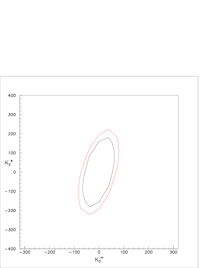
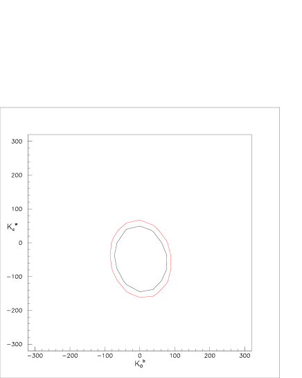
Figure 2: $2\sigma$ and $3\sigma$ contours from $e^{+}e^{-}\rightarrow W^{+}W^{-}\gamma\;$at $\sqrt{s}=200$ GeV in $k_{0}^{m}-k_{2}^{w}$ and the $k_{0}^{b}-k_{c}^{w}$ planes.

$$-1.35\;10^{-2}\;{\rm GeV}^{-2} < \frac{k_{0}^{b}}{\Lambda^{2}}<1.30\;10^{-2}\;{\rm GeV}^{-2}$$

$$-0.78\;10^{-2}\;{\rm GeV}^{-2} < \frac{k_{0}^{w}}{\Lambda^{2}}<0.73\;10^{-2}\;{\rm GeV}^{-2}$$

$$-1.20\;10^{-2}\;{\rm GeV}^{-2} < \frac{k_{0}^{m}}{\Lambda^{2}}<1.14\;10^{-2}\;{\rm GeV}^{-2}$$

$$-3.70\;10^{-2}\;{\rm GeV}^{-2} < \frac{k_{c}^{b}}{\Lambda^{2}}<2.50\;10^{-2}\;{\rm GeV}^{-2}$$

$$-2.69\;10^{-2}\;{\rm GeV}^{-2} < \frac{k_{c}^{w}}{\Lambda^{2}}<1.13\;10^{-2}\;{\rm GeV}^{-2}$$

$$-4.14\;10^{-2}\;{\rm GeV}^{-2} < \frac{k_{c}^{m}}{\Lambda^{2}}<1.77\;10^{-2}\;{\rm GeV}^{-2}$$

$$-1.44\;10^{-2}\;{\rm GeV}^{-2} < \frac{k_{1}^{w}}{\Lambda^{2}},\frac{k_{1}^{m}}{2\Lambda^{2}}<2.73\;10^{-2}\;{\rm GeV}^{-2}$$

$$-3.10\;10^{-2}\;{\rm GeV}^{-2} < \frac{k_{2}^{w}}{\Lambda^{2}},\frac{k_{2}^{m}}{2\Lambda^{2}}<3.20\;10^{-2}\;{\rm GeV}^{-2}$$

$$-2.82\;10^{-2}\;{\rm GeV}^{-2} < \frac{k_{3}^{w}}{\Lambda^{2}},\frac{k_{3}^{m}}{2\Lambda^{2}}<5.28\;10^{-2}\;{\rm GeV}^{-2}$$

$$-2.48\;10^{-2}\;{\rm GeV}^{-2} < \frac{a_{0}}{\Lambda^{2}}<2.39\;10^{-2}\;{\rm GeV}^{-2}\leftrightarrow-1.59\;10^{-2}\;{\rm GeV}^{-2}<\frac{k_{0}^{\gamma\gamma}}{\Lambda^{2}}<1.49\;10^{-2}\;{\rm GeV}^{-2}$$

We have also considered correlations for some specific combinations of couplings. As an illustration we show the correlations in the $k_{0}^{m}-k_{2}^{w}$ and the $k_{0}^{b}-k_{c}^{w}$ planes, see Fig. 2. In each instance all the other couplings are set to zero.

Figure 3: Distribution in the energy of the photon in $e^{+}e^{-}\rightarrow W^{+}W^{-}\gamma\;$due to the anomalous couplings $k_{0}^{b}$ and $k_{c}^{b}$ as compared to the tree-level ${\cal{S}}{\cal{M}}\;$. We have taken $k_{i}$ values that lead to a $3\sigma$ increase of the cross section as explained in the text. The $\pm$ are the positive and negative values given by Eq. (4.1).

We now turn to the distributions. As explained above we expect the distribution in the photon energy to be most revealing. This is borne out by our analysis where we do find that these couplings lead to energetic photons. To compare the various couplings we have chosen all $k_{i}$ such that they all give a $3\sigma$ increase in the $e^{+}e^{-}\rightarrow W^{+}W^{-}\gamma\;$cross section at $\sqrt{s}=200$ GeV with ${{\cal L}}=150$ fb^-1. First, we note that all $k_{0}^{i}$ give the same distribution. This is easily understood since we have found that these couplings interfered very little with the ${\cal{S}}{\cal{M}}\;$contribution and also because they all have the same Lorentz structure. However this is not the case for the other couplings. For this class of operators ($k_{i}^{j}\neq k_{0}^{j}$), we can, on the basis of the photon distribution discriminate, between the two signs of the couplings of a same operator (an effect of the interference with the ${\cal{S}}{\cal{M}}\;$) beside being able, in general, to differentiate between different operators, see Fig 3. Another interesting distribution to look at is the $p_{T}$ of the W, see Fig 4.

Figure 4: As in Fig. 3 but for the $p_{T}$ of one of the $W$’s.

4.2 $e^{+}e^{-}\;\rightarrow Z\gamma\gamma$ at LEP2

We take the same cuts on both photons as previously for $e^{+}e^{-}\rightarrow W^{+}W^{-}\gamma\;$. We then have a cross section which is sensibly the same as the one for $e^{+}e^{-}\rightarrow W^{+}W^{-}\gamma\;$: $.416$ pb. As explained above we basically are probing only two parameters $k_{0,1}^{i}$ and $k_{c,2,3}^{j}$. We have chosen to show $k_{0}^{b}$ and $k_{c}^{b}$ dependencies in Fig. 5. In $Z\gamma\gamma$, the $k_{0}$ couplings interfere more with the ${\cal{S}}{\cal{M}}\;$contributions than in $e^{+}e^{-}\rightarrow W^{+}W^{-}\gamma\;$.

Figure 5: Dependence of the $e^{+}e^{-}\;\rightarrow Z\gamma\gamma$ cross section at $\sqrt{s}=200$ GeV on the anomalous parameters $k_{0,c}$ with $\Lambda=M_{W}$. For the cuts on the photon refer to the text.

For the $3\sigma$ deviations we extract

$$-0.95\;10^{-2}\;{\rm GeV}^{-2} < \frac{k_{0}^{b},k_{0}^{w},k_{0}^{m},k_{1}^{b},k_{1}^{w},k_{1}^{m}}{\Lambda^{2}}<1.87\;10^{-2}\;{\rm GeV}^{-2}$$

$$-2.68\;10^{-2}\;{\rm GeV}^{-2} < \frac{k_{c}^{b},k_{c}^{w},k_{c}^{m},k_{2}^{b},k_{2}^{w},k_{2}^{m},k_{3}^{w},k_{3}^{m}}{\Lambda^{2}}<3.07\;10^{-2}\;{\rm GeV}^{-2}$$

$$-1.48\;10^{-2}\;{\rm GeV}^{-2} < \frac{a_{0}}{\Lambda^{2}}<3.01\;10^{-2}\;{\rm GeV}^{-2}$$ (4.37)

We now get limits on all couplings including $k_{1,2}^{b}$ which were not probed in $e^{+}e^{-}\rightarrow W^{+}W^{-}\gamma\;$. What is more interesting is that $e^{+}e^{-}\;\rightarrow Z\gamma\gamma$ sets slightly better limits on $k_{2,3}^{w,m}$. For the other couplings, combining both reactions improves the limits set by each process.

Once again the most typical distribution is that of the least energetic photon, as we can see from Fig. 6. Here again, given enough statistics it should be possible to disentangle between the two Lorentz structures.

Figure 6: Distribution in the least energetic photon in $e^{+}e^{-}\;\rightarrow\gamma\gamma Z$ due to the anomalous couplings $k_{0}^{b}$ and $k_{c}^{b}$. We have taken $k_{i}$ values that lead to a $3\sigma$ increase of the cross section as explained in the text. The $\pm$ are the positive and negative values given by Eq. (4.2).

4.3 Improvement at high energy

All these couplings will be much better probed as the energy increases. We have found that a linear collider running at $500$ GeV will improve these limits by as much as three orders of magnitude, especially for the $k_{0}$ couplings, see Fig. 7. To extract the $3\sigma$ limits we have assumed the same cuts as those at LEP2, we have only concentrated on the use of the $WW\gamma$ channel where we find the cross section to be $202.6$ fb. Choosing one operator from each of the three sets, ($k_{0},k_{c},k_{1}$), and assuming a total integrated luminosity of $500$ fb^-1, one will have the following constraints

$$-2.0\;10^{-5}\;{\rm GeV}^{-2} < \frac{k_{0}^{w}}{\Lambda^{2}}<0.6\;10^{-5}\;{\rm GeV}^{-2}$$

$$-8.1\;10^{-5}\;{\rm GeV}^{-2} < \frac{k_{c}^{m}}{\Lambda^{2}}<-5.0\;10^{-5}\;{\rm GeV}^{-2}\;\;{\rm and}\;\;-2.0\;10^{-5}\;{\rm GeV}^{-2}<\frac{k_{c}^{w}}{\Lambda^{2}}<1.2\;10^{-5}\;{\rm GeV}^{-2}$$

$$-9.0\;10^{-5}\;{\rm GeV}^{-2} < \frac{k_{2}^{w}}{\Lambda^{2}}<15.0\;10^{-5}\;{\rm GeV}^{-2}$$ (4.38)

We have also analysed how the sensitivity on the above limits changes if one increased the cut on the photon energy from $5$ GeV to $20$ GeV. The limits hardly change.

Note that we can in principle also use other channels, like for instance $e^{+}e^{-}\;\rightarrow WWZ$. However this channel is more conducive to tests on the $WWZZ$ couplings which appear at a lower order in the energy expansion in the context of the chiral Lagrangian and are thus more likely.

Figure 7: As in Fig. 1 but with $\sqrt{s}=500$ GeV. Here both the $\pm 3\sigma$ deviation with ${\cal{L}}=500$ fb^-1 are shown.

5 Remarks and conclusion

We have given an extensive list of ${\cal{C}}\;$and ${\cal{P}}\;$conserving quartic bosonic operators involving a photon and which may be probed at LEP2. Previous studies have considered only two operators beside a third which we have shown to be ${\cal{C}}{\cal{P}}\;$violating. We have shown how these structures can be embedded in a fully $SU(2)\times U(1)$ and $SU(2)_{c}$ globally invariant operators. We have derived limits on these couplings from $e^{+}e^{-}\rightarrow W^{+}W^{-}\gamma\;$and $e^{+}e^{-}\;\rightarrow Z\gamma\gamma$ at LEP2. When constraining the different structures so that we reproduce the contrived models considered by the OPAL collaboration [17] and in [7], our limits are consistent with theirs. We should however add a note of warning. The natural size of these couplings, $k_{i}^{j}$, should be of order unity for $\Lambda\sim 4\pi v\sim 3$TeV. Viewed this way the limits one will extract from LEP2 are not very meaningful and are much worse compared to the limits on the tri-linear couplings derived from LEP2. However the next generation of linear colliders can quite usefully constraint these operators, since we can gain as much as three-orders of magnitude compared to LEP2. Some order of magnitude on these non-renormalisable operators can also be set from their contributions to the low-energy precision measurements. However a study within a fully gauge invariant framework has not been done. A partial investigation [6] taking into account only two operators, with the restriction that no $WWZ\gamma$ and $ZZZ\gamma$ ensue, has been attempted, however the approach taken in [6] leads to these operators not decoupling in loop contributions and therefore cast a shadow on limits derived this way. For a discussion of how to treat the loop effects of the anomalous operator on low energy observables one should refer to [12, 18].

A Appendix

In [7] a $WWZ\gamma$ operator not listed in Eq.( 2) is also considered. Though $SU(2)_{c}$ symmetric, it is explicitly ${\cal{C}}{\cal{P}}\;$violating. The authors [7] take

$${{\cal L}}_{n}=-\frac{e^{2}}{16\Lambda^{2}}a_{n}\epsilon_{ijk}W^{i}_{\mu\alpha}W^{j}_{\nu}W^{k\;\alpha}F^{\mu\nu}$$ (A.1)

where the $W^{i}$ are the elements of $W$ triplet before mixing. Note that this Lagrangian differs from that of [6] by an overall $i$ factor which would make it non hermitian. Expanding in the physical fields one would get:

$${{\cal L}}_{n} = \;-i\;\frac{e^{2}}{16c_{W}\Lambda^{2}}a_{n}\left\{F_{\mu}^{\;\;\;\nu}\left[Z^{\mu\alpha}(W^{+}_{\alpha}W^{-}_{\nu}-W^{-}_{\alpha}W^{+}_{\nu})\right.\right.$$ (A.2)

$$+ \left.W^{+\;\mu\alpha}(W^{-}_{\nu}Z_{\alpha}-Z_{\nu}W^{-}_{\alpha})\;-\;W^{-\;\mu\alpha}(W^{+}_{\nu}Z_{\alpha}-Z_{\nu}W^{+}_{\alpha})\right]$$

Note now that properly going to the physical basis, the Lagrangian expressed in terms of the charged fields has an $i$ as required by hermiticity. In the passage from Eq. A.1 to Eq. A.2, a $i$ is missing in [7]. As explicit in Eq. A.2 this $i$ is crucial for hermiticity. On the other hand it is quite explicit also that this coupling violates ${\cal{C}}\;$and ${\cal{C}}{\cal{P}}\;$. Even if one had considered this coupling in computing $e^{+}e^{-}\;\rightarrow W^{+}W^{-}\gamma$, without any (transversely) polarized beams or the study of specific correlations in the decay products, this couplings does not interfere with the ${\cal{S}}{\cal{M}}\;$amplitudes. Therefore one only has a quadratic sensitivity on this anomalous coupling It is also interesting to write this Lagrangian in a gauge invariant manner. For instance in the chiral Lagrangian approach we may write:

$${{\cal L}}_{n}=i\frac{a_{4}^{{\rm CP}}}{\Lambda^{2}}g^{\prime}\;g{\rm Tr}\left(\tau_{3}{\mbox{\boldmath$B$}}_{\mu\nu}\right)\;{\rm Tr}\left({\mbox{\boldmath$W$}}^{\mu\alpha}\left[{\mbox{\boldmath$V$}}_{\nu},{\mbox{\boldmath$V$}}_{\alpha}\right]\right)$$ (A.3)

When written in terms of the physical fields this leads to the quartic couplings

$${{\cal L}}_{n}\rightarrow \frac{i}{2}\;e\;g^{2}\;g_{Z}\;\frac{a_{4}^{{\rm CP}}}{\Lambda^{2}}\left\{F_{\mu}^{\;\;\nu}\left[Z^{\mu\alpha}(W^{+}_{\alpha}W^{-}_{\nu}-W^{-}_{\alpha}W^{+}_{\nu})\right.\right.$$ (A.4)

$$+ \left.W^{+\;\mu\alpha}(W^{-}_{\nu}Z_{\alpha}-Z_{\nu}W^{-}_{\alpha})\;-\;W^{-\;\mu\alpha}(W^{+}_{\nu}Z_{\alpha}-Z_{\nu}W^{+}_{\alpha})\right]$$

$$- \left.\frac{s_{W}}{c_{W}}Z_{\mu}^{\;\;\nu}\left[W^{+\;\mu\alpha}(W^{-}_{\nu}Z_{\alpha}-Z_{\nu}W^{-}_{\alpha})\;-\;W^{-\;\mu\alpha}(W^{+}_{\nu}Z_{\alpha}-Z_{\nu}W^{+}_{\alpha})\right]\right\}$$

we would then have with the correct $i$,

$$a_{n}=\;-\;\frac{8}{s_{W}}g^{2}a_{4}^{{\rm CP}}$$ (A.5)

Note that this vertex when written in a gauge invariant manner also contributes to a $WWZZ$ vertex.

References

- [1] G. Bélanger and F. Boudjema, Phys. Lett. B288 (1992) 210.
- [2] M. Baillargeon, F. Boudjema, E. Chopin and V. Lafage, Z.Phys. C71 (1996) 431.hep-ph/9506396.
- [3] G. Bélanger and F. Boudjema, Phys. Lett. B288 (1992) 201.
- [4] K. Hagiwara, R. Peccei, D. Zeppenfeld and K. Hikasa Nucl. Phys. B282 (1987) 253.
- [5] G. Abu-Leil and W. J. Stirling, J. Phys. G21 (1995) 517.
- [6] O.J. P. Eboli, M.C. Gonzalez-Garcia and S. F. Novaes, Nucl. Phys. B411 (1994) 381.
- [7] W. J. Stirling and A. Werthenbach, Durham Preprint DTP/99/30. hep-ph/9903315. An analysis with final states has also been considered by these authors, DTP/99/62, hep-ph/9907235.
- [8] F. Boudjema, Invited talk at the Workshop on Physics and Experiments with Linear Colliders, Morioka, Japan, 1995, eds. A. Miyamoto et al.,, World Scientific, 1996, p. 199.
- [9] F. Boudjema and E. Chopin, Z. Phys. C73 (1996) 85.
- [10] M. Baillargeon, G. Bélanger and F. Boudjema, Nucl. Phys. B (1997) Nucl.Phys.B500 (1997) 224. hep-ph/9701372 .
-
[11]
OPAL Collaboration, Opal Physics Note PN410.
http://www.cern.ch/Opal/pubs/physnote/info/pn410.html. - [12] C.P. Burgess and D. London, Phys. Rev. Lett. 69 (1993) 3428; ibid Phys. Rev. D48 (1993) 4337.
- [13] T.Ishikawa, T.Kaneko, K.Kato, S.Kawabata, Y.Shimizu and K.Tanaka, KEK Report 92-19, 1993, The GRACE manual Ver. 1.0.
- [14] For a description of CompHep, see E.Boos et al., Proc.of the XXVIth Rencontres de Moriond, ed.by J.Tran Thanh Van, Editions Frontiers, 1991, p.501; E.Boos et al., Proc. of the Int. Conf. on Computing in High Energy Physics, ed.by Y.Watase, F.Abe, Universal Academy Press, Tokyo, 1991, p.391; E.Boos et al., Int. J. Mod. Phys. C5 (1994) 615; E.Boos et al., SNU CTP preprint 94-116, Seoul, 1994 (hep-ph/9503280).
-
[15]
A. Semenov. LanHEP — a package for automatic generation of Feynman
rules. User’s manual. INP MSU 96–24/431, Moscow, 1996; hep-ph/9608488
A. Semenov. Nucl.Inst.&Meth. A393 (1997) p. 293.
A. Semenov. Comp. Phys. Comm., Vol. 115 (1998) 124. - [16] A. Denner, S. Dittmaier, M. Roth and D. Wackeroth, Preprint BI-TP 99/10 and PSI-PR-99-12 hep-ph/9904472.
-
[17]
OPAL Collaboration, Opal Physics Note PN401.
http://www.cern.ch/Opal/pubs/physnote/info/pn401.html. - [18] K. Hagiwara, S. Ishihara, R. Szalapski and D. Zeppenfeld, Phys. Rev. D48 (1993) 2182.