[

UAB-FT-470

The $7/11$ rule: an estimate of $m_{\rho}/f_{\pi}$

Maarten F.L. Golterman Grup de Fisica Teorica and IFAE, Universitat Autonoma de Barcelona,
08193 Bellaterra (Barcelona), Spain
and
Department of Physics, Washington University,
St. Louis, MO 63130, USA[1]    Santiago Peris Grup de Fisica Teorica and IFAE, Universitat Autonoma de Barcelona,
08193 Bellaterra (Barcelona), Spain

Abstract

We derive an estimate for the ratio of the rho mass and the pion decay constant from an analysis of vector and axial-vector two-point functions using large-$N_{c}$, lowest-meson dominance and the operator product expansion, in the chiral limit. We discuss the extension of this analysis to the scalar and pseudoscalar sector. Furthermore, this leads to a successful parameter-free determination of the $L_{i}$ couplings of the chiral Lagrangian if an improved Nambu-Jona-Lasinio ansatz for Green functions is assumed at low energies.

pacs:

PACS numbers: 12.38.-t, 11.15.Pg, 11.55.Hx

]

I Introduction

The large-$N_{c}$ expansion [2] offers at present the only nonperturbative analytic approximation to QCD. This approximation is powerful enough to allow, for instance, a proof (within certain assumptions) of the expected pattern of chiral symmetry breaking [3]. In particular, for Green functions of color-singlet quark bilinears, the lowest order in this expansion corresponds to a theory of an infinite number of stable mesons.

At low energies there exists an effective field theory description in terms of what is called Chiral Perturbation Theory[4, 5] which corresponds to a systematic expansion of Green functions involving Goldstone mesons in powers of momenta and light quark masses. The resonance saturation of the $O(p^{4})$ Gasser–Leutwyler low-energy constants $L_{i}$ of Refs. [6, 7] can then be viewed as the matching between Chiral Perturbation Theory and large-$N_{c}$ QCD in the low-energy regime [8].

At high energies, QCD is described more efficiently by weak-coupling perturbation theory (enhanced with the Operator Product Expansion (OPE)). Unlike the low-energy counterpart, the matching between the high-energy regimes of large-$N_{c}$ QCD and perturbative QCD has been studied much less systematically, even though it has an enormous impact on our understanding of important problems such as weak matrix elements, see for instance Ref. [9].

Following Ref. [8] we will assume that the spectrum of this infinite tower of mesons can be reasonably approximated by just one resonance plus a sharp onset of the perturbative continuum at a scale $s_{0}$ (global duality) [10, 11]. Furthermore, in order to simplify the analysis, we will work in the chiral limit. The scale $s_{0}$ is fixed by the requirement of matching to the first term in the OPE[12]. Higher terms in the OPE then become fixed [13] in terms of the resonance parameters.

Concerning the reliability of this description we expect a certain “hierarchy” in this approach. First, at higher orders in the OPE, our simple description is likely to break down, but then the relative importance of the corresponding terms is also suppressed by higher powers of momenta. In practice, how far one can go is an open question, and may depend on the channel one is looking at. Second, one should expect that any linear combination of sum rules that is an order parameter of chiral symmetry (i.e. which would vanish were chiral symmetry unbroken) would be better approximated by our one-resonance-plus-continuum description than something that is not, as the former does not depend on our simple ansatz for the onset of the perturbative continuum, since it must cancel by definition in such combinations.

In Sect. II, we will consider two-point functions of the vector and axial-vector (nonsinglet) flavor currents. This will lead us to a new relation between the rho mass $m_{\rho}$, its electromagnetic decay constant $f_{\rho}$, and $f_{\pi}$. This relation turns out to work remarkably well when compared to experimental values of these parameters. In Sect. III, we discuss the extension of this type of analysis to the scalar and pseudo-scalar sector. While we find a relatively stable value for the scalar mass, this extension also exhibits the limitations of the approach, notably with respect to the chiral condensate. We make contact with a previous analysis based on a Nambu–Jona-Lasinio ansatz in Sect. IV, and summarize in Sect. V.

II Vectors

Although historically the two Weinberg sum rules [14] for the $\rho$ and $a_{1}$ mesons,

$$f_{\rho}^{2}m_{\rho}^{2}=f_{a_{1}}^{2}m_{a_{1}}^{2}+f_{\pi}^{2}\;,$$ (II.1)

$$f_{\rho}^{2}m_{\rho}^{4}=f_{a_{1}}^{2}m_{a_{1}}^{4}\;,$$ (II.2)

came before the large-$N_{c}$ expansion, they can be derived in our context in the following way [11]. One assumes that the vector-current two-point function $\Pi_{V}(q^{2})$, defined from

$$\Pi^{V}_{\mu\nu}(q) = i\int dx\;e^{iqx}\langle T(V_{\mu}(x)V^{\dagger}_{\nu}(0))\rangle$$ (II.3)

$$= (q_{\mu}q_{\nu}-g_{\mu\nu}q^{2})\Pi_{V}(q^{2})\;,$$ (II.4)

with $V_{\mu}(x)={\bar{d}}(x)\gamma_{\mu}u(x)$, can be described by (up to one subtraction)

$$\Pi_{V}(Q^{2}) = \int_{0}^{\infty}\frac{dt}{t+Q^{2}}\frac{1}{\pi}{\rm Im}\;\Pi_{V}(t)\;,$$ (II.5)

$$\frac{1}{\pi}{\rm Im}\;\Pi_{V}(t) = 2f_{\rho}^{2}m_{\rho}^{2}\delta(t-m_{\rho}^{2})$$ (II.7)

$$+\left(\frac{4}{3}\frac{N_{c}}{(4\pi)^{2}}+\dots\right)\theta(t-s_{0})\;,$$

where $f_{\rho}$ is the electromagnetic decay constant of the rho. The ellipsis represents higher-order perturbative corrections above a certain energy $\sqrt{s_{0}}$.

In the chiral limit, an analogous ansatz then holds for ${\rm Im}\;\Pi_{A}$ in terms of corresponding parameters for the $a_{1}$, defined from the axial current $A_{\mu}(x)={\bar{d}}(x)\gamma_{\mu}\gamma_{5}u(x)$, except that a term representing the pion, $2f_{\pi}^{2}(t)\delta(t)$, has to be added (we use the convention in which the experimental value of $f_{\pi}\simeq 93$ MeV). Since perturbative QCD does not see chiral symmetry breaking, one takes $s_{0}$ the same in the vector and axial channels.

One may now calculate $\Pi_{V,A}(Q^{2})$ for Euclidean momentum $Q$ from Eq. (II.7) and confront it with the OPE-result for large $Q^{2}$. One obtains the following set of relations [10, 12, 8]:

$$2f_{\rho}^{2}m_{\rho}^{2}-\frac{4}{3}\frac{N_{c}}{(4\pi)^{2}}s_{0} = 0\;,$$ (II.8)

$$-2f_{\rho}^{2}m_{\rho}^{4}+\frac{2}{3}\frac{N_{c}}{(4\pi)^{2}}s_{0}^{2} = \frac{1}{12\pi}\langle\alpha_{s}G_{\mu\nu}G^{\mu\nu}\rangle\;,$$ (II.9)

$$2f_{\rho}^{2}m_{\rho}^{6}-\frac{4}{9}\frac{N_{c}}{(4\pi)^{2}}s_{0}^{3} = -\frac{28}{9}\pi\alpha_{s}\langle\overline{\psi}\psi\rangle^{2}\;,$$ (II.10)

where the second term on the left-hand side of each of these equations comes from the leading term in the perturbative contribution to ${\rm Im}\;\Pi_{V}$, and the right-hand side is leading order in $\alpha_{s}$ and $1/N_{c}$. (Note that all terms are of the same order in $N_{c}$.) For the axial channel, one obtains

$$2f_{a_{1}}^{2}m_{a_{1}}^{2}+2f_{\pi}^{2}-\frac{4}{3}\frac{N_{c}}{(4\pi)^{2}}s_{0} = 0\;,$$ (II.11)

$$-2f_{a_{1}}^{2}m_{a_{1}}^{4}+\frac{2}{3}\frac{N_{c}}{(4\pi)^{2}}s_{0}^{2} = \frac{1}{12\pi}\langle\alpha_{s}G_{\mu\nu}G^{\mu\nu}\rangle\;,$$ (II.12)

$$2f_{a_{1}}^{2}m_{a_{1}}^{6}-\frac{4}{9}\frac{N_{c}}{(4\pi)^{2}}s_{0}^{3} = \frac{44}{9}\pi\alpha_{s}\langle\overline{\psi}\psi\rangle^{2}\;.$$ (II.13)

Combining Eqs. (II.8,II.11) and eliminating the gluon condensate between Eqs. (II.9,II.12) yields the two Weinberg sum rules in the form Eqs. (II.1,II.2).

One may expect these sum rules to be reasonably well satisfied, if the “onset” of perturbation theory occurs at a scale $\sqrt{s_{0}}$ (for which a phenomenological value can be calculated from Eq. (II.8)) above $m_{a_{1}}$, where presumably one may trust perturbative QCD. In addition, the sum rules do not depend on the gluon condensate. Eq. (II.9) then gives a phenomenological estimate for the gluon condensate as well, but this estimate may be less reliable, because it arises as the difference between two large numbers, one representing the low-energy, and the other representing the high-energy behavior of $\Pi_{V}$.

So far, we only reviewed a derivation of long-known results. However, we may carry this procedure one step further, and also eliminate the fermion condensate between Eqs. (II.10,II.13). Substituting the value of $s_{0}$ from Eq. (II.8), the result is a relation between $m_{\rho}$, $f_{\rho}$ and $f_{\pi}$:

$$\frac{1-\frac{3}{4}\frac{(4\pi)^{4}}{N_{c}^{2}}f_{\rho}^{4}}{(1-\frac{f_{\pi}^{2}}{f_{\rho}^{2}m_{\rho}^{2}})^{-1}-\frac{3}{4}\frac{(4\pi)^{4}}{N_{c}^{2}}f_{\rho}^{4}}=-\frac{7}{11}\;,$$ (II.14)

once $m_{a_{1}}$ and $f_{a_{1}}$ are eliminated using Weinberg’s sum rules.

The fact that the right-hand side of Eq. (II.14) is negative already leads to an interesting lower bound on $f_{\rho}$. First, note that $f_{\rho}^{2}m_{\rho}^{2}>f_{\pi}^{2}$, from Eq. (II.1). It then follows that the denominator of the left-hand side of Eq. (II.14) is larger than the numerator, and hence that the numerator has to be negative. In fact, we have

$$\frac{4}{3}\frac{N_{c}^{2}}{(4\pi)^{4}}<f_{\rho}^{4}<\frac{4}{3}\frac{N_{c}^{2}}{(4\pi)^{4}}\frac{1}{1-\frac{f_{\pi}^{2}}{f_{\rho}^{2}m_{\rho}^{2}}}\;,$$ (II.15)

and from the left inequality it follows that $f_{\rho}>0.148$. Using $f_{\pi}=87$ MeV (as an estimate of what its value would be in the chiral limit [5]), and $m_{\rho}=770$ MeV, the right inequality leads to $f_{\rho}<0.171$. This compares well with the experimental value $f_{\rho}=0.20$ if we take into account that we have used the large-$N_{c}$ (narrow resonance) and chiral approximations.

At this point we bring in yet another ingredient. Within our set of assumptions, another relation between $m_{\rho}$, $f_{\rho}$ and $f_{\pi}$ was previously obtained in Ref. [6] from the requirement that the pion electromagnetic form factor and axial form factor in $\pi\rightarrow e\nu_{e}\gamma$ satisfy unsubtracted dispersion relations:

$$f_{\rho}^{2}m_{\rho}^{2}=2f_{\pi}^{2}\;.$$ (II.16)

The right inequality now translates into $f_{\rho}<0.176$ (12% below the experimental value). In addition, this leads to a complete solution for all the parameters in the vector and axial channels in terms of $f_{\pi}$ (for $N_{c}=3$):

$$(4\pi f_{\rho})^{2}=4(4\pi f_{a_{1}})^{2}=\frac{10}{\sqrt{6}}\;,$$ (II.17)

$$m_{\rho}^{2}=m_{a_{1}}^{2}/2=\frac{\sqrt{6}}{5}(4\pi f_{\pi})^{2}\;,$$ (II.18)

and

$$\sqrt{s_{0}} = 4\pi f_{\pi}\;,$$ (II.19)

$$\langle\alpha_{s}G_{\mu\nu}G^{\mu\nu}\rangle = \frac{384}{5}\pi^{3}(5-2\sqrt{6})f_{\pi}^{4}\;,$$ (II.20)

$$\pi\alpha_{s}\langle\overline{\psi}\psi\rangle^{2} = \frac{768}{25}\pi^{4}f_{\pi}^{6}\;.$$ (II.21)

Using $f_{\pi}=87$ MeV, this gives $m_{\rho}=765$ MeV, $m_{a_{1}}=1082$ MeV, $f_{\rho}=0.16$ and $f_{a_{1}}=0.08$ which are remarkably good ($f_{a_{1}}$ is only poorly known experimentally).

The scale $\sqrt{s_{0}}=1.09$ GeV, slightly larger than the $a_{1}$ mass, is acceptable for the “onset” of perturbation theory. Even the condensates (which, as argued above, might be expected to fare less well) are reasonable: $\langle\alpha_{s}G_{\mu\nu}G^{\mu\nu}\rangle=0.014$ GeV⁴, and $\pi\alpha_{s}\langle\overline{\psi}\psi\rangle^{2}=(330~{}{\rm MeV})^{6}\simeq 13\times 10^{-4}$ GeV⁶. These numbers may for instance be compared to $\langle\alpha_{s}G_{\mu\nu}G^{\mu\nu}\rangle\simeq 0.048\pm 0.030$ GeV⁴ from Ref. [15], and to the combination $\pi\alpha_{s}\langle\overline{\psi}\psi\rangle^{2}\simeq(9\pm 2)\times 10^{-4}$ GeV⁶ as obtained from the fit to tau decays with the four-quark condensate recently performed in Ref. [16].

Using the two-loop running of $\alpha_{s}$ in the $\overline{MS}$ scheme,

$$\frac{\alpha_{s}(\mu)}{\pi}=\frac{A}{\log{\mu^{2}/\Lambda^{2}}}\left(1-B\frac{\log{\log{\mu^{2}/\Lambda^{2}}}}{\log{\mu^{2}/\Lambda^{2}}}\right)\;,$$ (II.22)

with $A=4/11$ and $B=102/121$ for $N_{c}=\infty$ and $A=4/9$, $B=64/81$ at $N_{c}=n_{f}=3$, one can now try to give an estimate for the value of the chiral condensate at the scale $s_{0}$. Using $\Lambda=300$–$400$ MeV and $N_{c}=3,\infty$, with $\alpha_{s}(\sqrt{s_{0}})/\pi=0.097$–$0.160$, one obtains

$$\langle\overline{\psi}\psi\rangle(\sqrt{s_{0}})=-(319\pm 13~{}{\rm MeV})^{3}\;,$$ (II.23)

where the error comes from the variation of $\alpha_{s}$.

At this point, we would like to make several comments about the stability of these results.

First, unlike the Weinberg sum rules, Eq. (II.14) does depend on higher-order corrections in $\alpha_{s}$ to the $s_{0}^{n}$ terms and the condensate terms in Eqs. (II.8–II.13). To leading order, $\alpha_{s}$-corrections to the $s_{0}^{n}$ terms can be incorporated by replacing $N_{c}/(4\pi)^{2}\to N_{c}(1+\alpha_{s}/\pi)/(4\pi)^{2}$ in Eq. (II.14) [17], which leads to a value of $f_{\rho}$ increased by a factor $1+\alpha_{s}/(2\pi)$. With the range of values for $\alpha_{s}$ above, this leads to an increase of at most 8%, or a decrease of $m_{\rho}$ by the same amount. There are also perturbative corrections to the ratio $-7/11$ in Eq. (II.14), which are not known to us. (There is no contribution from dimension 6 gluon condensates to the order considered[18].) However, recent attempts to extract information on the actual value of this ratio from $\tau$ decays data are consistent with a value not very different from $-7/11$ [19]. A change of the ratio $-7/11$ by 10% leads to a change of $f_{\rho}$ of about 1%. Note also that just the fact that the right-hand side of Eq. (II.14) is negative already led to an estimate $f_{\rho}=0.16(1)$, given the experimental value of the rho mass.

Second, one expects the estimates for the condensates to be less reliable than those for the $\rho$ and $a_{1}$ parameters as they arise from a subtle balance between the low- and high-energy ansätze for the vector and axial-vector two-point functions. We also remind the reader that, as a matter of principle, the gluon condensate has a physical meaning only in conjunction with the perturbative part and not in isolation [20]. All this, however, does not affect the Weinberg sum rules or the sum rule Eq. (II.14).

Third, one may expect that chiral corrections to the ratio $m_{\rho}/f_{\pi}$ are not large by noticing that the experimental value, 8.3, is close to $m_{K^{*}}/f_{K}=7.9$. (The difference between the two ratios should be due mainly to chiral corrections from the strange quark mass.)

III Scalars

In the previous section, we have applied some rather simple phenomenological assumptions to an analysis of vector and axial-vector two-point functions. This led to a complete and rather remarkable determination of the vector and axial-vector resonance parameters $m_{\rho,a_{1}}$ and $f_{\rho,a_{1}}$. Here we would like to explore what happens when we attempt to do the same in the (pseudo)scalar sector.

Again, we assume that, in the large $N_{c}$ and chiral limits, the scalar and pseudoscalar two-point functions, given by

$$\Pi_{S,P}(q)=i\int dx\;e^{iqx}\langle T(J_{S,P}(x)J_{S,P}^{\dagger}(0))\rangle\;,$$ (III.1)

where $J_{S}((x)={\overline{d}}(x)u(x)$ and $J_{P}(x)={\overline{d}}(x)\gamma_{5}u(x)$, can be described by

$$\Pi_{S,P}(Q^{2})=\int_{0}^{\infty}\frac{dt}{t+Q^{2}}\frac{1}{\pi}{\rm Im}\;\Pi_{S,P}(t)+{\rm subtractions}\;,$$ (III.2)

with

$${\rm Im}\;\Pi_{S}(t) = 16B^{2}c_{m}^{2}\delta(t-m_{S}^{2})+\frac{N_{c}}{(4\pi)^{2}}\kappa 2t\theta(t-{\hat{s}}_{0})\;,$$ (III.3)

$${\rm Im}\;\Pi_{P}(t) = 2B^{2}f_{\pi}^{2}\delta(t)+16B^{2}d_{m}^{2}\delta(t-m_{P}^{2})$$ (III.5)

$$+\frac{N_{c}}{(4\pi)^{2}}\kappa 2t\theta(t-{\hat{s}}_{0})\;,$$

where we use the notation of Ref. [7]. The scale ${\hat{s}}_{0}$ is not necessarily the same as the scale $s_{0}$ in the vector sector. To first order in perturbation theory, the factor $\kappa$ is known to contain very large $\alpha_{s}$ corrections[21]

$$\kappa=1+\frac{\alpha_{s}(\mu)}{\pi}\left(\frac{17}{3}-2\log{\frac{t}{\mu^{2}}}\right)\;,$$ (III.6)

which is the reason why we do not discard it right from the beginning. Eq. (III.6) is only valid at $N_{c}=3$. However, as we will see in the numerical analysis that follows, these large $\alpha_{s}$ corrections turn out to have no significant impact on the numerical results.

For large Euclidean $Q^{2}$, we may again confront $\Pi_{S,P}(Q^{2})$ calculated from Eqs. (III.2-III.6) with the OPE result of Ref. [22]. Taking $\mu=\sqrt{{\hat{s}}_{0}}$, and equating inverse powers of $Q^{2}$, one finds, with $B=-\langle\overline{\psi}\psi\rangle/f_{\pi}^{2}$, in the large $N_{c}$ and chiral limits

$$16B^{2}c_{m}^{2}-\frac{N_{c}}{16\pi^{2}}{\hat{s}}_{0}^{2}\kappa_{1}({\hat{s}}_{0}) = \frac{1}{8\pi}\langle\alpha_{s}G_{\mu\nu}G^{\mu\nu}\rangle\;,$$ (III.7)

$$-16B^{2}c_{m}^{2}m_{S}^{2}+\frac{N_{c}}{24\pi^{2}}{\hat{s}}_{0}^{3}\kappa_{2}({\hat{s}}_{0}) = -\frac{22}{3}\pi\alpha_{s}\langle\overline{\psi}\psi\rangle^{2}$$ (III.8)

in the scalar sector, and

$$2B^{2}f_{\pi}^{2}+16B^{2}d_{m}^{2}-\frac{N_{c}}{16\pi^{2}}{\hat{s}}_{0}^{2}\kappa_{1}({\hat{s}}_{0})=$$ (III.9)

$$\!\!\!\!\!\!\!\!\!\!\!\!\!\frac{1}{8\pi}\langle\alpha_{s}G_{\mu\nu}G^{\mu\nu}\rangle\;,$$ (III.10)

$$-16B^{2}d_{m}^{2}m_{P}^{2}+\frac{N_{c}}{24\pi^{2}}{\hat{s}}_{0}^{3}\kappa_{2}({\hat{s}}_{0})=$$ (III.11)

$$\!\!\!\!\!\!\!\!\!\!\!\!\!\frac{14}{3}\pi\alpha_{s}\langle\overline{\psi}\psi\rangle^{2}$$ (III.12)

in the pseudoscalar sector. The leading perturbative corrections $\kappa_{1}$ and $\kappa_{2}$ stem from the $\kappa$ factor in Eq. (III.6), and read

$$\kappa_{1}({\hat{s}}_{0}) = 1+\frac{20}{3}\frac{\alpha_{s}(\sqrt{{\hat{s}}_{0}})}{\pi}\;,$$ (III.13)

$$\kappa_{2}({\hat{s}}_{0}) = 1+\frac{19}{3}\frac{\alpha_{s}(\sqrt{{\hat{s}}_{0}})}{\pi}\;.$$ (III.14)

At this point, let us discuss how we may try to explore these equations. In order to eliminate the dependence on the gluon condensate and the perturbative terms, we might choose to first consider combinations that are order parameters of chiral symmetry, and look at the differences (III.7)$-$(III.9) and (III.8)$-$(III.11), i.e. [23, 24]:

$$8c_{m}^{2}-8d_{m}^{2}-f_{\pi}^{2} = 0\;,$$ (III.15)

$$B^{2}c_{m}^{2}m_{S}^{2}-B^{2}d_{m}^{2}m_{P}^{2} = {3\over 4}\pi\alpha_{s}\langle\overline{\psi}\psi\rangle^{2}\;.$$ (III.16)

Given the values of $\pi\alpha_{s}\langle\overline{\psi}\psi\rangle^{2}$ (for instance from the vector sector, cf. Eq. (II.21)) and $m_{S,P}$ we may solve these equations for $c_{m}$, $d_{m}$, which are then still logarithmically dependent on the scale ${\hat{s}}_{0}$ (through $\alpha_{s}$). The additional equation is provided by Eq. (III.7) (or equivalently Eq. (III.9)), and we obtain a solution for $c_{m}$, $d_{m}$ and ${\hat{s}}_{0}$. It turns out that the solution is very insensitive to the gluon condensate (see below). This leaves us with the question of what values to use for $m_{S,P}$. We will assume that $m_{P}$ corresponds to the mass of the $\pi(1300)$, which is firmly established in the Particle Data Tables. As is well known, the situation in the scalar sector is much less understood (for a recent discussion, see Ref. [25]). Therefore, instead of directly guessing a value for the scalar mass, we will add an extra equation. Within our set of assumptions, the low-energy constant $L_{8}$ [5] is determined by [7]

$$L_{8}=\frac{c_{m}^{2}}{2m_{S}^{2}}-\frac{d_{m}^{2}}{2m_{P}^{2}}\;.$$ (III.17)

The experimental value is $L_{8}=0.9(3)\times 10^{-3}$ [26].

Note that we have not used Eq. (III.8) (or, equivalently, Eq. (III.11)) separately yet.

Let us now consider solutions. Taking $f_{\pi}=87$ MeV, $\Lambda_{\overline{MS}}=372$ MeV [28], $m_{P}=1300$ MeV, and $L_{8}=0.0009$, and using the results Eqs. (II.20,II.21) for the condensates, we obtain

$$c_{m}=41~{}{\rm MeV}, d_{m}=27~{}{\rm MeV},$$ (III.18)

$$m_{S}=0.86~{}{\rm GeV}, \sqrt{{\hat{s}}_{0}}=2.16~{}{\rm GeV}\;.$$ (III.19)

Note that the $\pi$(1300) “decouples from” $L_{8}$ in that it only gives a very small contribution to it.

Except for ${\hat{s}}_{0}$, these results are rather stable. In order to demonstrate this, we will vary one input at a time and see how the values of $c_{m}$, $d_{m}$, $m_{S}$ and ${\hat{s}}_{0}$ change.

Varying the gluon condensate from 0 to 10 times the value given in Eq. (II.20) has no significant impact on the solution. Changing $\Lambda_{\overline{MS}}$ to 300 MeV changes these numbers by at most about 5%. Even changing the $\alpha_{s}$ corrections in the $\kappa$ factor by a huge factor such as 10, or omitting the $\alpha_{s}$ correction altogether, does not significantly change these numbers (except the value of ${\hat{s}}_{0}$).

Changing $m_{P}$, and even more so $L_{8}$, has a bigger effect (note that these effects are related through Eq. (III.17)). Taking $m_{P}$ from 1400 MeV to 1200 MeV (keeping $L_{8}=0.0009$) leads to

$$38~{}{\rm MeV}< c_{m} <46~{}{\rm MeV}\;,$$ (III.20)

$$22~{}{\rm MeV}< d_{m} <34~{}{\rm MeV}\;,$$ (III.21)

$$0.84~{}{\rm GeV}< m_{S} <0.90~{}{\rm GeV}\;,$$ (III.22)

$$2.08~{}{\rm GeV}< \sqrt{{\hat{s}}_{0}} <2.32~{}{\rm GeV}\;.$$ (III.23)

We found no solution for $m_{P}\stackrel{{\scriptstyle<}}{{\sim}}1$GeV. Similarly, changing $L_{8}$ from 0.0012 to 0.0006 (keeping $m_{P}=1300$ MeV) gives

$$36~{}{\rm MeV}< c_{m} <81~{}{\rm MeV}\;,$$ (III.24)

$$19~{}{\rm MeV}< d_{m} <74~{}{\rm MeV}\;,$$ (III.25)

$$0.71~{}{\rm GeV}< m_{S} <1.20~{}{\rm GeV}\;,$$ (III.26)

$$2.02~{}{\rm GeV}< \sqrt{{\hat{s}}_{0}} <3.25~{}{\rm GeV}\;.$$ (III.27)

Although all these solutions satisfy the difference (III.8)$-$(III.11), they do not satisfy Eq. (III.8) or Eq. (III.11) separately. With the value of $\pi\alpha_{s}\langle\overline{\psi}\psi\rangle^{2}$ from the vector sector, there does not appear to exist any reasonable solution to the four equations Eqs. (III.7-III.11) (for any reasonable choice of $m_{P}$). Perhaps another indication of this problem is the value of ${\hat{s}}_{0}$, which is substantially larger than the value of $s_{0}$ found in the vector sector. At $\Lambda_{\overline{MS}}=372$ MeV, one has $\alpha_{s}({\hat{s}}_{0})\approx 0.09(0.07)$, to be compared with $\alpha_{s}(s_{0})\approx 0.15(0.12)$ for $N_{c}=n_{f}=3$ ($N_{c}=\infty$). This makes a difference of about 20% in the value of $\langle\overline{\psi}\psi\rangle$. If we solve the same set of equations, but with Eq. (III.8) replacing Eq. (III.7), we obtain, instead of the result (III.18) and (III.19),

$$c_{m}=40~{}{\rm MeV}, d_{m}=26~{}{\rm MeV},$$ (III.28)

$$m_{S}=0.86~{}{\rm GeV}, \sqrt{{\hat{s}}_{0}}=1.64~{}{\rm GeV}\;.$$ (III.29)

Resonance parameters stay the same; the only thing that changes is the value of ${\hat{s}}_{0}$. This is an example of a point we made in the Introduction: our simple ansatz for the onset of the perturbative continuum seems to make Eq. (III.8) and Eq. (III.11) incompatible (but, see below).

However, since the continuum cancels in the difference, the combination (III.8)$-$(III.11) does lead to a solution. Of course, the lack of a solution to both Eqs. (III.8) and Eq. (III.11) may merely mean that our spectrum is too simple to reproduce the physics of dimension-six operators in the OPE. However, even in the present case, we may appreciate how stable resonance parameters seem to be by means of the following little exercise. First notice that, up to now, we have been using the value of $\pi\alpha_{s}\langle\overline{\psi}\psi\rangle^{2}$ obtained in the (axial)vector sector. Just as we studied the effect of the variation of other inputs earlier, this brings us now to the sensitivity of the solution in the scalar-pseudoscalar sector to the value of the quark condensate. It is interesting to see what happens if we lower, by fiat, the value of this four-fermion condensate. (The value of $\langle\overline{\psi}\psi\rangle$ in Eq. (II.23) is rather high in comparison with other phenomenological estimates.) As it turns out, we happen to find a solution for $m_{S,P}$, $c_{m}$, $d_{m}$ and ${\hat{s}}_{0}$ from the whole set of equations (Eqs. (III.7-III.11,III.17)) if we lower the value of Eq. (II.21) by a fudge factor 11:

$$c_{m}=51~{}{\rm MeV}, d_{m}=41~{}{\rm MeV},$$ (III.30)

$$m_{S}=0.92~{}{\rm GeV}, m_{P}=1.13~{}{\rm GeV},$$ (III.31)

$$\sqrt{{\hat{s}}_{0}}=1.14~{}{\rm GeV}\;.$$ (III.32)

(For reduction factors smaller than 11, we find ${\hat{s}}_{0}<m_{P}^{2}$, which is not acceptable: the basic assumption was that two-point functions can be described by a small number of narrow resonances below an energy scale $s_{0}$, and perturbative QCD above that scale.) What we learn is that even in this case the solution (in particular the scalar mass) stays roughly in the neighborhood of the resonance parameters found in Eqs. (III.18,III.19).

While it is clear that the scalar sector is less simple than the vector sector in this approach, one interesting fact emerges from this section: it seems likely that there exists a scalar resonance with mass between 700 and 1200 MeV in the large-$N_{c}$ and chiral limits.

IV The $L_{i}$ couplings

In Ref. [8] it was shown how an extended Nambu–Jona-Lasinio [29] ansatz for Green’s functions in QCD can be improved to restrict the parameters of the lowest-meson dominance approximation to the large-$N_{c}$ limit in a way which is compatible with several examples of the OPE. The final outcome of this analysis was a determination of all the $L_{i}$’s leading at large $N_{c}$ in terms of the ratio $f_{\pi}/m_{\rho}$. At $N_{c}=3$, they read [8]:

$$6L_{1}= 3L_{2}=-\frac{8}{7}L_{3}=4L_{5}=8L_{8}=\frac{3}{4}L_{9}=-L_{10}$$ (IV.1)

$$=\frac{3}{8}\frac{f_{\pi}^{2}}{m_{\rho}^{2}}\;.$$ (IV.2)

Since we can now use Eq. (II.18) to fix this ratio to be

$$\frac{3}{8}\frac{f_{\pi}^{2}}{m_{\rho}^{2}}=\frac{15}{8\sqrt{6}}\frac{1}{16\pi^{2}}\;,$$ (IV.3)

Eqs. (IV.2,IV.3) lead to a parameter-free determination for the $L_{i}$ couplings.

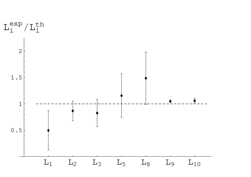
FIG. 1.: Ratios of the experimental values and those obtained from Eq.  (IV.2,IV.3) for the $O(p^{4})$ constants $L_{i}$. The error bars represent the experimental errors.

This is plotted in Fig. 1, where we use $\mu=m_{\rho}$ for the renormalization scale in these couplings to estimate their experimental values. The error bars represent only the errors in the experimental values, and one should keep the uncertainty in the choice of renormalization scale in mind while considering Fig. 1. For instance, if we change the scale from $m_{\rho}$ to 1 GeV, the couplings $L_{9}$ and $L_{10}$ change by $-6$%, resp. 8%, which is more than the experimental error. Of course, a more precise knowledge about the scale $\mu$ at which the matching takes place would be required for a more detailed analysis (which would necessarily go beyond leading order in $1/N_{c}$).

V Discussion

Let us summarize what we have learned from this simple large-$N_{c}$ inspired model for vector and scalar two-point functions.

First, we showed that the usual “large-$N_{c}$ plus lowest-meson dominance” derivation of the two Weinberg sum rules can be extended to give us a third sum rule, Eq. (II.14), relating vector masses and couplings. Like the first two sum rules, this sum rule is nontrivial because of the fact that chiral symmetry is spontaneously broken, with nonvanishing $f_{\pi}$ and $\langle\overline{\psi}\psi\rangle$.

This new sum rule can be combined with Eq. (II.16) to express $m_{\rho}$, $m_{a_{1}}$ and $f_{\rho}$, $f_{a_{1}}$ in terms of $f_{\pi}$. We find $m_{\rho}/f_{\pi}=8.8$, and $f_{\rho}=0.16$, to be compared with the experimental values $m_{\rho}/f_{\pi}=8.3$, and $f_{\rho}=0.20$. (The $a_{1}$ parameters then follow from the Weinberg sum rules in the usual way.) The agreement between our values and the experimental ones is very good, considering that the $1/N_{c}$ and chiral expansions are ingredients of our analysis.

The scale for the onset of perturbation theory comes out slightly higher than the $a_{1}$ mass. One also obtains values for the gluon and chiral condensates. Note, however, that the three sum rules are derived by eliminating the condensates, and that our results for $m_{\rho}$ and $f_{\rho}$ are therefore independent of their values.

Then, we presented a similar analysis for the scalar and pseudoscalar two-point functions. An important qualitative difference is the fact that, in this case, restricting ourselves to the same set of condensates in the OPE, only four (Eqs. (III.7-III.11)) instead of six (Eqs. (II.8-II.13) are obtained. This is related to the fact that in the scalar sector, two subtractions are needed in Eq. (III.2), while only one subtraction is necessary in the vector sector, because of current conservation.

As a consequence of this, our analysis for the scalars does in principle depend on the gluon and chiral condensates. The sensitivity to the value of the gluon condensate turns out to be very small. This is not true for the chiral condensate, $\langle\overline{\psi}\psi\rangle$. We find, in particular, that the value of the chiral condensate obtained from the vectors, is too large to satisfy all equations in the scalar sector with reasonable values for all parameters. This is consistent with the fact that this value of the condensate is also on the high side in comparison with other estimates. Interestingly, we find that the value of the scalar mass is very insensitive to the value of the chiral condensate. It depends, however, on the value of $L_{8}$ (which we used as input). We would like to emphasize that one should not try to identify this large-$N_{c}$ scalar resonance with the broad $\sigma$ [25] appearing in $\pi-\pi$ scattering, as the latter is more likely a $\pi-\pi$ bound state [27], whose dynamics is subleading at large $N_{c}$, and cannot give rise to a leading large-$N_{c}$ coupling like $L_{8}$.

To summarize, in all cases we considered, we find a scalar mass between $\sim 0.7$ and $\sim 1.2$ GeV[30], where the spread is mostly due to the error in the experimental value of $L_{8}$.

Finally we use our Eq. (II.18) in combination with the analysis of Ref. [8] to produce a parameter-free determination of the Gasser–Leutwyler $L_{i}$ couplings in the ${\cal O}(p^{4})$ chiral Lagrangian, see Fig. 1. The overall agreement for the seven $L_{i}$ couplings is remarkable.

Acknowledgements:

We thank M. Knecht, A. Pich, E. de Rafael, A. Gonzalez-Arroyo and F. Yndurain for discussions and comments; and A.A. Andrianov and D. Espriu for pointing out a numerical error in a previous version of the manuscript.

MG thanks the Physics Department of the University of Washington, where part of this work was carried out, for hospitality. MG is supported in part by a Fellowship of the Spanish Government SAB1998-0171 and as a US Department of Energy Outstanding Junior Investigator. SP is supported by the research project CICYT-AEN98-1093 of the Spanish Government and by TMR, EC-Contract No. ERBFMRX-CT980169 (EURODA$\phi$NE).

REFERENCES

- [1] Permanent address.
- [2] G. ’t Hooft, Nucl. Phys. B72 (1974) 461; E. Witten, Nucl. Phys. B 160 (1979) 57.
- [3] S. Coleman and E. Witten, Phys. Rev. Lett. 45 (1980) 100.
- [4] S. Weinberg, Physica A 96 (1979) 327.
- [5] J. Gasser and H. Leutwyler, Annals of Phys. (NY) 158 (1984) 142; Nucl. Phys. B250 (1985) 465.
- [6] G. Ecker et al., Phys. Lett. B223 (1989) 425.
- [7] G. Ecker et al., Nucl. Phys. B321 (1989) 311.
- [8] S. Peris, M. Perrottet and E. de Rafael, JHEP05 (1998) 011.
- [9] M. Knecht, S. Peris and E. de Rafael, Phys. Lett. B443 (1998) 255; Phys. Lett. B457 (1999) 227.
- [10] M.A. Shifman, A.I. Vainshtein and V.I. Zakharov, Nucl. Phys. B147 (1979) 385; Nucl. Phys. B147 (1979) 448.
- [11] E. de Rafael, hep-ph/9802448; lectures delivered at Les Houches 1997.
- [12] R.A. Bertlmann, G. Launer and E. de Rafael, Nucl. Phys. B250 (1985) 61.
- [13] M. Knecht and E. de Rafael, Phys. Lett. B424 (1998) 335.
- [14] S. Weinberg, Phys. Rev. Lett. 18 (1967) 507.
- [15] F.J. Yndurain, hep-ph/9903457.
- [16] M. Davier, A. Hocker, L. Girlanda and J. Stern, Phys. Rev. D58 (1998) 096014.
- [17] S.G. Gorishny, A.L. Kataev and S.A. Larin, Phys. Lett. B259 (1991) 144; L.R. Surguladze and M.A. Samuel, Phys. Rev. Lett. 66 (1991) 560, and references therein.
- [18] W. Hubschmid and S. Mallik, Nucl. Phys. B207 (1982) 29.
- [19] ALEPH Collaboration, Eur. Phys. J. C4 (1998) 409; see also A. Pich, “ Tau Physics”, hep-ph/9704453, in “ Heavy Flavours II”, eds. A.J. Buras and M. Lindner, World Sci. 1997 and references therein. We are most grateful to A. Pich for informative discussions on this point.
- [20] See for instance, G. Martinelli and C.T. Sachrajda, Nucl. Phys. B478 (1996) 660.
- [21] C. Becchi, S. Narison, E. de Rafael and F. Yndurain, Z. Phys. C8 (1981) 335.
- [22] M. Jamin and M. Münz, Z. Phys.C66 (1995) 633.
- [23] M. Knecht and E. de Rafael, unpublished.
- [24] A.A. Andrianov, D. Espriu and R. Tarrach, Nucl. Phys. B533 (1998) 429. See also A.A. Andrianov and D. Espriu, hep-ph/9906459.
- [25] M. Pennington, Talk at the Workshop on Hadron Spectroscopy, WHS99, Frascati, March 1999, hep-ph/9905241.
- [26] See for instance A. Pich hep-ph/9806303, lectures delivered at Les Houches 1997. For a recent determination of and see M. Davier et al., Phys. Rev. D58 (1998) 096014
- [27] See for instance, J.A. Oller and E. Oset hep-ph/9809337, to appear in Phys. Rev. D, and references therein.
- [28] M. Davier and A. Hocker, Phys. Lett. B419 (1998) 419.
- [29] See for instance, J. Bijnens, Phys. Rep. 265 (1996) 369.
- [30] Recently this result has also been obtained independently in Ref. [24]. Some of the views of these authors are however different from ours.