Abstract

We study the third order pion–nucleon scattering amplitude obtained from heavy baryon chiral perturbation theory inside the Mandelstam triangle. We reconstruct the pion–nucleon amplitude in the unphysical region by use of dispersion relations and determine the pertinent low–energy constants by a fit to this amplitude. A detailed comparison with values obtained from phase shift analysis is given. Our analysis leads to a pion–nucleon $\sigma$–term of $\sigma(0)=40\,$MeV based on the Karlsruhe partial wave analysis. We have repeated the same procedure using the latest solution of the VPI group and find a much larger value for $\sigma(0)$.

1 Introduction

A detailed understanding of elastic pion–nucleon scattering in the low energy region allows for precise tests of the chiral QCD dynamics. Recently, this process has been investigated to third order in heavy baryon chiral perturbation theory by various groups. At that order, one has to deal with tree graphs and one loop diagrams. At second and third order, there are in total four and five so–called low–energy constants, respectively, which have to be determined by comparison to data. The loop contribution only depends on the weak pion decay constant $F=92.4$ MeV and the axial–vector coupling $g_{A}=1.26$. In ref.[1], particular combinations of threshold and subthreshold parameters were found which do not depend on the dimension three low–energy constants (LECs). Also, it was shown that the ensuing numerical values of these dimension two LECs, called $c_{i}$, can be understood in terms of resonance exchange. In ref.[2], the threshold parameters based on the Karlsruhe–Helsinki analysis together with the pion–nucleon $\sigma$–term were used to fix the nine LECs. The results for the $c_{i}$ were in good agreement with the ones obtained in [1]. The amplitude given in [2] was used later to obtain S– and P–wave phase shifts below the first resonance [3]. The most systematic study was performed in ref.[4], where the S– and P–wave partial wave amplitudes from three different analyses were used (in the physical region and in the range of the lowest existing data) to fit the LECs. However, chiral perturbation theory is expected to yield the most reliable predictions for $s$ (the center–of–mass energy squared) and $t$ (the squared invariant four–momentum transfer) lying inside the Mandelstam triangle (depicted in fig.1), for essentially two reasons. First, in this region the scattering amplitude is purely real and it is well known that at a given order in the chiral expansion, the real part is in general more precisely determined than the corresponding imaginary part (since the latter only starts at one loop order). Second, in the interior of the Mandelstam triangle the kinematical variables $t$ and $(s-u)/4m$ take their smallest values. As this region is unphysical, there is no direct access by experimental data. By the use of dispersion relations this problem can be circumvented. This is done here. First, using data from phase shift analysis we construct the pion–nucleon amplitude inside the Mandelstam triangle. We then use the chiral third order amplitude constructed in [4] to determine the 8 LECs under consideration by a best fit as described below and compare their numerical values with the ones obtained previously. The ninth LEC is fixed by the value of the pion–nucleon coupling constant used in our analysis. We expect a more precise determination of the dimension two LECs since to the order we are working, we are not sensitive to the $1/m$ corrections to the dimension three LECs (which are known to be important in the determination of the $c_{i}$, compare e.g. the values obtained in [5] with the ones of refs.[1, 2, 4].). We remark that Höhler [6] has stressed that one should also compare directly the analytical form of the pion–nucleon amplitude obtained by different means. We refer to his work for a detailed comparison between the dispersive and the chiral representation. Also, it is known that in some small regions the heavy baryon amplitude converges slowly. This can be traced back to the fact that the strict heavy baryon limit tends to modify the analytical structure of the $\pi N$ amplitude. These effects can be dealt with by subtracting from the amplitudes the full Born terms, since the latter generate the singularities (such an effect also appears in the discussion of the nucleon electromagnetic form factors, see e.g. [7, 8, 9]). It is important to stress that this subtraction procedure is not arbitrary since the subthreshold expansion of the $\pi N$ invariant amplitudes is usually formulated by subtracting the Born terms to avoid their rapid variations in the appropriate kinematical variables. Another way of circumventing this problem is to stick to a relativistic formulation of the matter fields, as recently proposed in ref.[10] since in that way all strictures from analyticity are automatically fulfilled. Here, however, we are concerned with the comparison of the $\pi N$ amplitude obtained in heavy baryon chiral perturbation theory (HBCHPT) since in this framework the most precise predictions for the threshold parameters have been obtained and we wish to explore the consistency of these calculations at the order they have been performed. In contrast to previous investigations, we confine ourselves to the inside of the Mandelstam triangle for the reasons mentioned above.

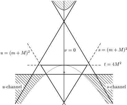
Figure 1: Mandelstam plane. The Mandelstam triangle is the inside of the thick lines. The star marks the so–called “ideal point” explained in sec. 4.

The manuscript is organized as follows. Some formalism pertaining to elastic pion–nucleon scattering pertinent to our investigation is given in sec. 2. In sec. 3 we construct the invariant amplitudes inside the Mandelstam triangle by use of dispersion relations. The chiral perturbation theory amplitudes are fitted to these dispersive amplitudes in sec. 4. Further results on subthreshold parameters and the $\sigma$–term are discussed in sec. 5. The summary and conclusions follow in sec. 6.

2 Formal aspects of elastic pion–nucleon scattering

Consider elastic pion–nucleon scattering,

$$\pi^{a}(q_{1})+N(p_{1})\to\pi^{b}(q_{2})+N(p_{2})~{},$$ (1)

with ‘$a,b$’ (cartesian) pion isospin indices and $q_{i}$, $p_{i}$ the four–momenta of the pions and the nucleons, respectively. The scattering amplitude is usually decomposed in terms of the four invariant functions $A^{\pm}(s,t)$ and $B^{\pm}(s,t)$ (where the superscript ‘$\pm$’ refers to the isoscalar/isovector part),

$$T^{ba}_{\pi N}(s,t) = T_{\pi N}^{+}(s,t)\,\delta^{ba}+T_{\pi N}^{-}(s,t)\,\frac{1}{2}[\tau^{b},\tau^{a}]~{},$$

$$T^{\pm}_{\pi N}(s,t) = \bar{u}(p_{2},\lambda_{2})\,\biggl{[}A^{\pm}(s,t)+\frac{1}{2}(q_{2}+q_{1})^{\mu}\gamma_{\mu}\,B^{\pm}(s,t)\biggr{]}\,u(p_{1},\lambda_{1})~{},$$ (2)

with $\sqrt{s}$ the cms energy and $t=(q_{1}-q_{2})^{2}$ the invariant momentum transfer squared. The $\lambda_{i}$ ($i=1,2)$ denote the helicities of the incoming/outgoing nucleon. In what follows, we also need the linear combinations related to the physical channels $\pi^{+}p\to\pi^{+}p$ and $\pi^{-}p\to\pi^{-}p$. These are related to the isospin amplitudes by

$$X^{\pm}(s,t)=\frac{1}{2}\biggl{(}X_{-}(s,t)\pm X_{+}(s,t)\biggr{)}~{},\quad X=\{A,B\}~{}.$$ (3)

The invariant amplitudes fulfill the crossing relations

$$A^{+}(s,t,u) = A^{+}(u,t,s)~{},$$

$$B^{-}(s,t,u) = B^{-}(u,t,s)~{},$$

$$A^{-}(s,t,u) = -A^{-}(u,t,s)~{},$$

$$B^{+}(s,t,u) = -B^{+}(u,t,s)~{}.$$ (4)

For heavy baryon chiral perturbation theory, it is more natural to work directly with the non–spin–flip and spin–flip amplitudes $g^{\pm}(\omega,t)$ and $h^{\pm}(\omega,t)$, respectively. For a discussion of this point, see [4]. Then, the $\pi N$ scattering amplitude takes the form

$$T^{ba}_{\pi N}(\omega,t) = \biggl{(}\frac{E+m}{2m}\biggr{)}\,\biggl{\{}\delta^{ba}\Big{[}g^{+}(\omega,t)+i\vec{\sigma}\cdot(\vec{q}_{2}\times\vec{q}_{1}\,)\,h^{+}(\omega,t)\Big{]}$$ (5)

$$\qquad\quad+i\,\epsilon^{bac}\tau^{c}\Big{[}g^{-}(\omega,t)+i\vec{\sigma}\cdot(\vec{q}_{2}\times\vec{q}_{1}\,)\,h^{-}(\omega,t)\Big{]}\biggr{\}}$$

with $\omega$ the pion cms energy,

$$\omega=\sqrt{\frac{(s-m^{2}+M^{2})^{2}}{4s}}~{},$$ (6)

$E=(\vec{q\,}^{2}+m^{2})^{1/2}$ the nucleon energy and the pion momenta

$$\vec{q\,}_{1}^{2}=\vec{q\,}_{2}^{2}\equiv\vec{q\,}^{2}\equiv q^{2}={(s-M^{2}-m^{2})^{2}-4m^{2}M^{2}\over 4s}\quad.$$ (7)

The relations between the invariant amplitudes $A^{\pm},B^{\pm}$ and $g^{\pm},h^{\pm}$ is

$$g^{\pm}(\omega,t)={C_{4}A^{\pm}(\omega,t)-C_{2}B^{\pm}(\omega,t)\over C_{1}C_{4}-C_{2}C_{3}}~{},$$ (8)

$$h^{\pm}(\omega,t)={-C_{3}A^{\pm}(\omega,t)+C_{1}B^{\pm}(\omega,t)\over C_{1}C_{4}-C_{2}C_{3}}~{},$$ (9)

with the coefficient functions $C_{i}$ $(i=1,\ldots,4$) given by

$$C_{1} = {\frac{{m^{2}}-{M^{2}}-m\,\omega+m\,{\sqrt{{m^{2}}-{M^{2}}+{{\omega}^{2}}}}}{2\,({m^{2}}-{M^{2}})}}~{},$$

$$C_{2} = \frac{1}{4\,\left(m^{2}-M^{2}\right)}\left\{4\,{m^{2}}\,{M^{2}}-4\,{M^{4}}-{m^{2}}\,t+{M^{2}}\,t-4\,{m^{3}}\,\omega\right.$$

$$\left.+m\,t\,\omega+4\,{M^{2}}\,{{\omega}^{2}}-m\,\left(t+4\,m\,\omega-4\,{M^{2}}\right)\,{\sqrt{{m^{2}}-{M^{2}}+{{\omega}^{2}}}}\right\}~{},$$

$$C_{3} = {\frac{1}{2\,\left(\omega+{\sqrt{{m^{2}}-{M^{2}}+{{\omega}^{2}}}}\right)}}~{},$$

$$C_{4} = {\frac{\left(m+{\sqrt{{m^{2}}-{M^{2}}+{{\omega}^{2}}}}\right)\,\left(4\,m\,\left(m+{\sqrt{{m^{2}}-{M^{2}}+{{\omega}^{2}}}}\right)-t\right)}{4\,\left({m^{2}}-{M^{2}}+m\,\omega+{{\omega}^{2}}+\left(m+\omega\right)\,{\sqrt{{m^{2}}-{M^{2}}+{{\omega}^{2}}}}\right)}}~{}.$$ (10)

This form differs from the one in [4] in that it is explicitly given in terms of $\omega$ and $t$ and also it is more directly applicable for considering processes in regions other than the physical $s$–channel domain. Note that these coefficient functions should not be expanded in $1/m$ when one performs the chiral expansion. Finally, we will also use the crossing–symmetric variable $\nu=(s-u)/4m$, the scattering angle in the center–of–mass system in the $s$-channel, $\cos\theta=1+t/2q^{2}$, and sometimes denote the cms energy by $W$, i.e. $s=W^{2}$. We also need the subthreshold expansion of the invariant amplitudes with the pseudovector Born terms subtracted (as indicated by the “bar”) [11]

$$\bar{X}=\sum_{m,n}x_{mn}\,\nu^{2m+k}\,t^{n}~{},\quad X=\{A^{\pm},B^{\pm}\}~{},$$ (11)

with $k=1\,(0)$ if the function considered is odd (even) in $\nu$. The Taylor–coefficients $x_{mn}$ are the so–called subthreshold parameters. For a more detailed account of the pertinent kinematics, we refer to the monograph [11].

3 Construction of the invariant amplitudes inside the Mandelstam triangle using dispersion relations

In the next step, we use dispersion relations to construct the $\pi N$ amplitude inside the Mandelstam triangle. The Mandelstam triangle is the interior of the region bounded by the three lines $s=(M+m)^{2}$, $u=(M+m)^{2}$ and $t=4M^{2}$ in the Mandelstam plane, see fig. 1. Dispersion relations for $\pi N$ scattering have been studied in great detail in axiomatic field theory in the last thirty years [12, 11]. Using analyticity, unitarity, and crossing symmetry one obtains dispersive relations for the scattering amplitudes of the form

$${\rm Re}~{}A^{\pm}(\nu,t) = {1\over\pi}{\int\!\!\!\!\!\!-}_{\nu_{\rm thr}}^{\infty}\!\!\!\!\!{\rm Im}~{}A^{\pm}(\nu^{\prime},t)\biggl{\{}\frac{1}{\nu^{\prime}-\nu}\pm\frac{1}{\nu^{\prime}+\nu}\biggr{\}}\,d\nu^{\prime}~{},$$ (12)

$${\rm Re}~{}B^{\pm}(\nu,t) = {1\over\pi}{\int\!\!\!\!\!\!-}_{\nu_{\rm thr}}^{\infty}\!\!\!\!\!{\rm Im}~{}B^{\pm}(\nu^{\prime},t)\biggl{\{}\frac{1}{\nu^{\prime}-\nu}\mp\frac{1}{\nu^{\prime}+\nu}\biggr{\}}\,d\nu^{\prime}+\frac{g^{2}}{2m}\left(\frac{1}{\nu_{B}-\nu}\mp\frac{1}{\nu_{B}+\nu}\right)~{},$$

with $\nu_{\rm thr}=M+t/(4m)$ and $\nu_{B}=(t-2M^{2})/(4m)$. Note that the nucleon Born terms contribute only to $B^{\pm}(\nu,t)$. Here

$$f^{2}=\frac{g^{2}}{4\pi}\left(\frac{M}{2m}\right)^{2}\simeq 0.079$$ (14)

is the pion–nucleon coupling constant squared. There is some debate about its actual value, some analysis favoring a somewhat smaller value, $f^{2}\simeq 0.075$, as discussed below. However, to be consistent with refs.[1, 2, 4], which mostly use the Karlsruhe phase shifts and therefore the value given in eq.(14), we also use the large value for $f^{2}$. Note that in addition we consider an analysis favouring a smaller value for $f^{2}$ later on. We mention that it seems clear that the imaginary part of the amplitudes $A^{-},B^{\pm}$ fall off sufficiently fast so that no subtraction is needed. This might also be true for $A^{+}$, see e.g. [13]. However, to precisely determine the subthreshold parameters related to $A^{+}$, we perform a subtraction for the amplitude $A^{+}$ [11],

$${\rm Re}~{}A^{+}(\nu,t)={\rm Re}~{}A^{+}(\nu=0,t)+{2\nu^{2}\over\pi}{\int\!\!\!\!\!\!-}_{\nu_{\rm thr}}^{\infty}\,{{\rm Im}~{}A^{+}(\nu^{\prime},t)\over\nu^{\prime}(\nu^{\prime 2}-\nu^{2})}\,d\nu^{\prime}~{},$$ (15)

where the first term on the right–hand–side of eq.(15) is the subtraction function. This will be discussed in more detail below. Note also that the influence of any high energy contribution is damped further in the once subtracted dispersion relation for $A^{+}(\nu,t)$.

The absorptive parts of the amplitudes in the dispersive integrals are broken up into two parts: a) the low energy part with laboratory momenta $k_{\rm lab}\leq 6\,$GeV and b) the high energy part. The first is constructed by partial waves of the Karlsruhe group (KA84) [14]. We note that there has been considerable criticism of these partial wave amplitudes recently (see e.g. the proceedings of MENU 97 [15]), however, at present no other analysis exist which consistently includes data from threshold to the highest available energies (for example, the VPI group uses the Karlsruhe analysis for $k_{\rm lab}$ above 2.1 GeV [6]). In our numerical analysis we work with the S– to K–wave approximation of the physical amplitudes $A_{\pm}(\nu,t)$ and $B_{\pm}(\nu,t)$, i.e. (for clarity, we only display the S– and P–wave contributions here. The ellipsis stands for the contributions from the higher partial waves.)

$${A_{+}(\nu,t)\over 4\pi} = {W+m\over E+m}\biggl{\{}f_{0+}^{3/2}(\nu)+3\cos\theta f_{1+}^{3/2}(\nu)\biggr{\}}-{W-m\over E-m}\biggl{\{}f_{1-}^{3/2}(\nu)-f_{1+}^{3/2}(\nu)\biggr{\}}~{}+\ldots,$$

$${A_{-}(\nu,t)\over 4\pi} = {W+m\over 3(E+m)}\biggl{\{}f_{0+}^{3/2}(\nu)+2f_{0+}^{1/2}(\nu)-3\cos\theta\bigl{[}f_{1+}^{3/2}(\nu)-2f_{1+}^{1/2}(\nu)\bigr{]}\biggr{\}}$$ (17)

$$- {W-m\over 3(E-m)}\biggl{\{}f_{1-}^{3/2}(\nu)+2f_{1-}^{1/2}(\nu)-f_{1+}^{3/2}(\nu)-2f_{1+}^{1/2}(\nu)\biggr{\}}~{}+\ldots,$$

$${B_{+}(\nu,t)\over 4\pi} = {1\over E+m}f_{0+}^{3/2}(\nu)+\biggl{\{}{3\cos\theta\over E+m}-{1\over E-m}\biggr{\}}f_{1+}^{3/2}(\nu)+{1\over E-m}f_{1-}^{3/2}(\nu)~{}+\ldots,$$ (18)

$${B_{-}(\nu,t)\over 4\pi} = {1\over 3(E+m)}\biggl{\{}f_{0+}^{3/2}(\nu)+2f_{0+}^{1/2}(\nu)+3\cos\theta\bigl{[}f_{1+}^{3/2}(\nu)+2f_{1+}^{1/2}(\nu)\bigr{]}\biggr{\}}$$ (19)

$$+ {1\over 3(E-m)}\biggl{\{}f_{1-}^{3/2}(\nu)+2f_{1-}^{1/2}(\nu)-f_{1+}^{3/2}(\nu)-2f_{1+}^{1/2}(\nu)\biggr{\}}~{}+\ldots~{},$$

yielding the desired amplitudes $A^{\pm},B^{\pm}$ by eq.(3). To construct e.g. the amplitude $B_{+}(\nu,t)$, we need the partial waves with the appropriate quantum numbers from S31 up to K315 (in the usual notation $l_{2I,2j}$). The pertinent partial wave amplitudes $f_{l\pm}^{I}(\nu)$ for total isospin $I=1/2,3/2$, pion–nucleon angular momentum $l$ and total angular momentum $j=l\pm 1/2$ are given in terms of the phase shifts $\delta_{l\pm}^{I}(\nu)$ and inelasticities $\eta_{l\pm}^{I}(\nu)$ via

$$f_{l\pm}^{I}(\nu)={1\over 2iq}\bigl{\{}\eta_{l\pm}^{I}(\nu)\exp\delta_{l\pm}^{I}(\nu)-1\bigr{\}}~{}.$$ (20)

Figure 2: Argand plot of $A^{+}(\nu,t=0)$ for $k_{\rm lab}\leq 6\,$GeV. All units are appropriate powers of the pion mass.

Figure 3: Argand plot of $\omega\,B^{-}(\nu,t=0)$ for $k_{\rm lab}\leq 6\,$GeV. All units are appropriate powers of the pion mass.

The corresponding Argand diagrams for $A^{+}$ and $\omega B^{-}$ in the low energy region are shown in figs. 2 and 3, respectively. These reproduce the ones given by Höhler and collaborators with sufficient accuracy for our later purposes, compare with the corresponding figures in ref.[16]. For the high energy part of the amplitudes $A^{-}$ and $B^{-}$ we assume a reggeized $\rho$–meson exchange in the $t$–channel of the charge exchange process $\pi^{-}p\to\pi^{0}n$ to be the sole component of the amplitude [11], e.g.

$${\rm Im}~{}B_{R}^{-}(\omega,t)=D_{0}\,\alpha(t)\{\alpha(t)+1\}\biggl{(}\frac{\omega}{\omega_{0}}\biggr{)}^{\alpha(t)-1}~{},$$ (21)

with $D_{0}=38.9\,$mb, $\omega_{0}=1\,$GeV and the Regge slope is parameterized via $\alpha(t)=0.56+1.08\cdot t$ [17].

In the present work we will make use of the amplitudes along the lines $\nu=0$ and $t=2M^{2}/3$ (and also $t=0$) to map out the interior of the Mandelstam triangle (cf. fig. 1). The choice of this particular value of $t$ is justified in the next section. Consequently, $B^{-}(0,t)$ and the subtraction function $A^{+}(0,t)$ will be of special interest to us. We remark that $A^{-}(0,t)$ and $B^{+}(0,t)$ vanish because of crossing symmetry. $A^{+}(0,t)$ is reconstructed by approximating the real and imaginary part of $A^{+}$ in the physical region of the $s$–channel by the available partial waves. Inverting eq.(15) then yields $A^{+}(0,t)$. The result is shown in fig. 4. We remark that this amplitude fulfills the Adler consistency condition

$$A^{+}(\nu=0,t=M^{2},q_{1}^{2}=0,q_{2}^{2}=M^{2})\simeq\frac{g^{2}}{m}$$ (22)

within one percent. Since physical pions do not have vanishing four–momentum, one expects a deviation from this relation of the order of $M^{2}/(4\pi F)^{2}\simeq 1.5\%$. $B^{-}(0,t)$ is obtained from eq.(3). The $\nu$–dependence of the amplitudes is evaluated in a similar fashion by keeping $t$ fixed at the value given above.

Figure 4: The subtraction function $A^{+}(\nu=0,t)$. The solid (dotted) line refers to the KA84 (VPI SP99) partial–wave analysis.

So far, we have used the KA84 phase shift analysis. We are aware that some of the data entering that analysis are now considered inconsistent. Consequently, we will also use the latest version of the VPI phase shift analysis, called SP99 [18], for our calculations. We note that the VPI group uses dispersion relations only for some of the amplitudes and in a certain energy region, different from the Karlsruhe method. Based on the VPI SP99 phases, we have constructed the amplitudes $A^{\pm},B^{\pm}$ as described before. We refrain from showing the corresponding figures, but we remark that the Adler consistency condition is then violated by 10 percent. The corresponding subtraction function is also shown in fig.4 by the dotted curve. Of course, one has to account for the smaller value of the pion–nucleon coupling constant used by the VPI group, $f^{2}\simeq 0.076$. The Adler consistency relation is of importance for the precise determination of the amplitudes when the Born terms are subtracted. We believe that for making accurate statements on small quantities like the pion–nucleon $\sigma$ term, it is mandatory to fulfill such constraints as e.g. the Adler condition to the expected accuracy as explained before.

4 Chiral perturbation theory amplitudes inside the Mandelstam triangle

We now turn to the comparison with the chiral amplitude. For that, it is important to study the dependence of the various invariant amplitudes on the pertinent LECs. We give here the explicit expressions for the counterterm amplitudes taken from ref.[4] (in terms of $t$ and $\omega$)

$$g^{+}_{\rm ct} = \frac{c_{2}\,\omega}{mF^{2}}\Bigl{[}4\omega^{2}-4M^{2}+t\Bigr{]}+\frac{1}{F^{2}}\left[-4c_{1}M^{2}+2c_{2}\omega^{2}+c_{3}(2M^{2}-t)\right]~{},$$ (23)

$$g^{-}_{\rm ct} = \frac{c_{4}\,\omega\,t}{2mF^{2}}+\frac{2\omega}{F^{2}}(2M^{2}-t)\,(\bar{d}_{1}+\bar{d}_{2})+\frac{4\omega^{3}}{F^{2}}\,\bar{d}_{3}+\frac{8\omega\,M^{2}}{F^{2}}\,\bar{d}_{5}$$ (24)

$$\qquad\qquad+\,\frac{g_{A}}{F^{2}}\frac{M^{2}}{\omega}(2\omega^{2}-2M^{2}+t)\,\bar{d}_{18}$$

$$h^{+}_{\rm ct} = \frac{2\omega}{F^{2}}\,(\bar{d}_{14}-\bar{d}_{15})+\frac{g_{A}}{F^{2}}\frac{2M^{2}}{\omega}\,\bar{d}_{18}~{},$$ (25)

$$h^{-}_{\rm ct} = \frac{c_{4}\,\omega}{mF^{2}}+\frac{c_{4}}{F^{2}}~{},$$ (26)

to facilitate the later discussion. The $\nu$–dependence can be worked out using the fact that $\omega$ and $\nu$ are related via

$$\nu=\frac{1}{4m}\,(2s+t-2M^{2}-2m^{2})~{},$$ (27)

and using eq.(6). Note that most of the LECs appear only in one particular invariant amplitude, e.g. $c_{1},c_{2},c_{3}$ are fixed entirely from varying $g^{+}(\omega,t)$ inside the Mandelstam triangle. Only $c_{4}$ and $\bar{d}_{18}$ appear in two different amplitudes. In particular, we expect that most of the dimension three LECs cannot be pinned down accurately, since they only appear in $g^{-}_{\rm ct}$ with small prefactors. This expectation is borne out by the results given below. Furthermore, to this order in the chiral expansion we are not sensitive to the $1/m$ corrections to the $\bar{d}_{i}$. Such terms are known to play an important role in the precise determination of the dimension two LECs, compare e.g. the values obtained in ref.[5] with the ones in refs.[1, 2, 4]. It should be noted that the amplitudes given in [4] are valid for $\omega>M,t<0$. Therefore, when working inside the Mandelstam triangle, one has to ensure the correct analytic continuation to the unphysical region $\omega<M$ of the complex–valued one–loop contributions of $g^{\pm}$ and $h^{\pm}$ by use of [1]

$$\sqrt{1-x^{2}}=-i\,\sqrt{x^{2}-1}~{},\quad\arcsin x=\frac{\pi}{2}+i\ln\left(x+\sqrt{x^{2}-1}\right)~{}.$$ (28)

A similar statement holds for the continuation to $t>0$. We use the tree and one–loop amplitudes explicitly given in [4] but refrain from spelling them out here.

The chiral amplitudes to order $O(q^{3})$ do not have the correct analytic structure inside the Mandelstam triangle. This is in part due to the Taylor expansion of the lowest order amplitude in powers of $m^{-1}$. To avoid this problem, it is necessary to neglect the tree contributions and the counter terms $\sim g_{A}$. This holds in particular for the tree graphs with insertions $\sim\bar{d}_{18}$. The latter allow one to use the physical value of the pion–nucleon coupling constant (instead of its value in the chiral limit) in the tree graphs, which are responsible for the incorrect analytic behaviour. This procedure is equivalent to working with the quantities $\bar{A}^{+}\equiv A^{+}-g^{2}/m$ and so on instead of $A^{\pm},B^{\pm}$ in eqs.(8),(9). This way, all the contributions due to $\bar{d}_{18}$ drop out and the latter has to be calculated in a different way, e.g. by the so–called Goldberger-Treiman discrepancy (i.e the deviation from the Goldberger-Treiman relation):

$$g_{\pi N}=\frac{g_{A}m}{F_{\pi}}\left(1-\frac{2M_{\pi}^{2}\bar{d}_{18}}{g_{A}}\right)~{}.$$ (29)

In the present work we compare the chiral amplitudes with their dispersive counterparts in a small region inside the Mandelstam triangle. More precisely, we concentrate on two regions. The first of these is concentrated around the point $\nu=0$ and $t=2M^{2}/3$, the so–called “ideal point”. In the chiral limit, where the pions are massless, the ideal point is given by $\nu=t=0$ and the constraint $s+t+u=2m_{0}^{2}$ has to be fulfilled, with $m_{0}$ the nucleon mass in the chiral limit. Since we are considering physical nucleons and physical pions, the ideal point is shifted to $t\simeq 2M^{2}/3$ because now $s+t+u=2m^{2}+2M^{2}$. We consider two fits, which span the following regions within the Mandelstam triangle

$${\rm Fit~{}1:} {\rm around}~{}\nu=0,~{}t=0~{}$$ (30)

$${\rm with}~{}\{-0.5~{}M^{2}\leq t\leq 0.5~{}M^{2}\,,45.7M^{2}\leq s\leq 46.7M^{2}\}~{},$$

$${\rm Fit~{}2:} {\rm around}~{}\nu=0,~{}t=2M^{2}/3~{}$$ (31)

$${\rm with}~{}\{-0.3~{}M^{2}\leq t\leq 0.7~{}M^{2}\,,45.35M^{2}\leq s\leq 46.35\}~{},$$

This means that for both fits we cover the range of one pion mass squared in the two independent Mandelstam variables. A larger range cannot be accounted for by the third order chiral amplitudes. We have convinced ourselves that decreasing these ranges by a factor of two does not change our results. Note that for the fits along the line $\nu=0$, a simplification arises. Due to crossing symmetry and eqs.(8),(9), each of the amplitudes $\bar{g}^{\pm},\bar{h}^{\pm}$ depends on only one of the invariant amplitudes $\bar{A}^{\pm},\bar{B}^{\pm}$. E.g. the non-spin-flip amplitude $\bar{g}^{+}(\nu=0,t)$ is related to the modified subtraction function $\bar{A}^{+}(\nu=0,t)$ via

$$\bar{g}^{+}(0,t) = \frac{C_{4}}{C_{1}C_{4}-C_{2}C_{3}}\bar{A}^{+}(0,t)~{}.$$ (32)

A fit to each of the dispersive amplitudes $\bar{g}^{\pm}(\nu,t),\bar{h}^{\pm}(\nu,t)$ at 21 equidistantly separated points in the two directions of fixed $\nu$ and fixed $t$ in the regions given in eq.(30) yields the following values for the LECs (we give here the averaged values obtained from fit 1 and fit 2 together, the individual results are displayed and discussed below):

$$c_{1} = (-0.81\pm 0.12)~{}\mbox{GeV}^{-1}~{},\quad c_{2}=(8.43\pm 56.9)~{}\mbox{GeV}^{-1}~{},$$

$$c_{3} = (-4.70\pm 1.16)~{}\mbox{GeV}^{-1}~{},\quad c_{4}=(3.40\pm 0.04)~{}\mbox{GeV}^{-1}~{}.$$ (33)

The errors given are the the ones from the two fits added in quadrature. The errors for each fit have been determined from the square root of the diagonal elements of the error matrix. We note that there is a sizeable variation in the precision with which the dimension two LECs are determined. It is expected that the isovector amplitudes are more accurately predicted at third order by chiral perturbation theory since the isoscalar amplitudes vanish to leading order in the chiral expansion. That is also the reason why the LEC $c_{4}$ is more precisely pinned down than the LECs $c_{1,2,3}$. In table 1 we compare the values of the dimension two LECs for fit 1 and fit 2 separately with previous determinations.

$c_{i}$	Fit 1	Fit 2	Ref.[1]	Ref.[2]	Ref.[4] (Fit 1)
1	$-0.81\pm 0.15$	$-0.80\pm 0.07$	$-0.93\pm 0.10$	$-0.94\pm 0.06$	$-1.23\pm 0.16$
2	$9.35\pm 66.7$	$7.52\pm 45.0$	$3.34\pm 0.20$	$3.20\pm 0.10$	$3.28\pm 0.23$
3	$-4.69\pm 1.34$	$-4.70\pm 0.95$	$-5.29\pm 0.25$	$-5.40\pm 0.06$	$-5.94\pm 0.09$
4	$3.40\pm 0.04$	$3.40\pm 0.04$	$3.63\pm 0.10$	$3.47\pm 0.06$	$3.47\pm 0.05$

Table 1: The dimension two LECs $c_{1,2,3,4}$ in GeV^-1 from our determination based on the KA84 phase shifts compared to previous ones using also information from $\pi N$ scattering in the physical region and the $\sigma$–term.

In ref.[1], (sub)threshold parameters and the $\sigma$–term (i.e. quantities free of dimension three LECs) were used, while in ref.[2] the $c_{i}$ and dimension three LECs were determined from a fit to threshold parameters of the Karlsruhe–Helsinki group [19]. Finally, the determination in ref.[4] (fit 1 therein) used only the available low–energy KA84 phase shifts for pion laboratory momenta in the range from 40 to 97 MeV. The results for $c_{1}$, $c_{3}$ and $c_{4}$ are very consistent for all the different determinations. The exception is our value for $c_{2}$, which is essentially an undetermined quantity. There reason for that is that in the amplitude $g^{+}$, which is small, the LECs $c_{1}$ and $c_{3}$ are weighted with factors of $M^{2}$, whereas the term $\sim c_{2}$ is proportional to $\omega^{2}$ (to leading order in the $1/m$) and this quantity is suppressed by a factor of 10 compared to $M^{2}$ in the region around the center of the Mandelstam triangle. As a consequence, we can not make a precise prediction for the combination $c^{+}=c_{2}+c_{3}-2c_{1}$, which can also be deduced from pion scattering off deuterium [20]. One could, however, turn the argument around and use the value of $c^{+}$ determined in ref.[20], $c^{+}=-0.09\pm 0.37\,$GeV^-1. Neglecting the uncertainties in $c_{1}$ and $c_{3}$, this leads to

$$c_{2}=(2.99\pm 0.37)~{}\mbox{GeV}^{-1}~{},$$ (34)

which is consistent with the other determinations compiled in table 1. It is also possible to pin down the LECs $c_{1,3,4}$ from the long–range part of the proton–proton interaction based on the chiral two–pion exchange potential. This has been done in ref.[21] and leads to results consistent with the ones found here and in previous works. The values obtained in ref.[21] are $c_{1}=-0.76(7)$, $c_{3}=-5.08(28)$ and $c_{4}=4.70(70)$ (all in GeV^-1). Finally, we remark that the errors we quote (compare eq.(4) and table 1) must be handled with care: to our knowledge, there is no error analysis available for the KA84 phase shifts and elasticities. Thus, it is impossible to give reliable errors for the dispersive amplitudes inside the Mandelstam triangle. In the present work we assume an error of 10 % for the amplitudes of interest. In this sense our errors are arbitrary. Stated differently, using other errors does not change the central values but the uncertainties deduced from the corresponding error matrix.

We now turn to the dimension three LECs. We have found that if we fit along lines of fixed $\nu$ or fixed $t$, they can be pinned down with good precision. However, the so determined values are not mutually consistent. The reason for this lies in the fact that the third order amplitude employed here is not sufficiently precise to describe the small contributions from ${\cal L}_{\pi N}^{(3)}$ accurately. In table 2 we compare our results for the $\bar{d}_{i}$. Only the combination $\bar{d}_{14}-\bar{d}_{15}$ comes out consistent for the determinations within the regions given by fits 1 and 2, respectively. Note, however, that the overall description of the amplitude $h^{+}$ is fairly poor, so that this determination of $\bar{d}_{14}-\bar{d}_{15}$ has to be taken with some caution (even though the uncertainty in this LEC from the fits is tiny). It appears that the $1/m^{2}$ corrections with fixed coefficients and the $c_{i}/m$ terms are more important than the genuinely new operators of dimension three. Also shown in table 2 are results from previous determinations determined by fitting to threshold parameters and phase shifts. It would be valuable to have additional information on these LECs, say from a study of elastic pion–nucleon scattering to fourth order in the chiral expansion or from the reaction $\pi N\to\pi\pi N$.

$\bar{d}_{i}$	Fit 1	Fit 2	Ref.[2]	Ref.[4] (Fit 1)
1+2	$3.33\pm 0.01$	$-1.91\pm 0.14$	$2.4\pm 0.3$	$3.06\pm 0.21$
3	$-152.3\pm 0.24$	$98.16\pm 6.90$	$-2.8\pm 0.6$	$-3.27\pm 0.73$
5	$-0.11\pm 0.01$	$-0.20\pm 0.01$	$1.4\pm 0.3$	$0.45\pm 0.42$
14-15	$0.96\pm 0.00$	$0.93\pm 0.00$	$-6.1\pm 0.6$	$-5.65\pm 0.41$

Table 2: The dimension three LECs $\bar{d}_{i}$ in GeV^-2 (and combinations thereof) from our determination compared to previous ones using information from $\pi N$ scattering in the physical region.

Using now the SP99 phases as input to construct the amplitudes and redo the fit, we find (taking into account the different value for the $\pi N$ coupling constant used by the VPI group)

$$\begin{array}[]{lcccr}c_{1}&=&(-3.00\ldots-2.96)~{}{\rm GeV}^{-1}&&[(-1.53\pm 0.18)~{}{\rm GeV}^{-1}]~{},\\ c_{2}&=&(-9.51\ldots 7.22)~{}{\rm GeV}^{-1}&&[(3.22\pm 0.25)~{}{\rm GeV}^{-1}]~{},\\ c_{3}&=&(-6.63\ldots-6.20)~{}{\rm GeV}^{-1}&&[(-6.20\pm 0.09)~{}{\rm GeV}^{-1}]~{},\\ c_{4}&=&(3.39\ldots 3.40)~{}{\rm GeV}^{-1}&&[(3.51\pm 0.04)~{}{\rm GeV}^{-1}]~{},\\ \bar{d}_{14}+\bar{d}_{15}&=&(0.92\ldots 0.93)~{}{\rm GeV}^{-2}&&[(-1.53\pm 0.18)~{}{\rm GeV}^{-2}]~{},\\ \end{array}$$ (35)

where we have given the range based on fits 1,2 as described above. The numbers in the square brackets are the results of fit 3 of ref.[4] based on the VPI SP98 solution. The uncertainties of the so determined LECs are very similar to the ones obtained based on the KA84 partial waves. Again, we note that $c_{2}$ cannot be determined. Notice in particular the very large value for $c_{1}$, which will be commented on below. The value for $c_{4}$ is in perfect agreement with the one found before, i.e. the amplitude $h^{-}$ is the same for the KA84 and VPI SP99 analysis. For $\bar{d}_{1}+\bar{d}_{2}$, $\bar{d}_{3}$ and $\bar{d}_{5}$ we encounter the same problems as discussed before and therefore refrain from giving the corresponding numbers. We note, however, that the values obtained for these LECs are very similar to the ones obtained for the Karlsruhe phase shifts, compare table 2. For the reasons discussed in sec.3, we consider the determination based on the KA84 phases more consistent (despite the fact that a part of the data set used in the Karlsruhe analysis is now outdated). As noted before, the dimension three LECs can mostly not be determined precisely. For achieving a better precision, one has to go to fourth order and fit in a larger region inside the Mandelstam triangle.

5 Results and discussion

In HBCHPT the quantities of interest are expressed in terms of the LECs. Explicit expressions for e.g. the subthreshold parameters and the $\sigma$-term $\sigma(0)$ are given in [1, 4]. For convenience, we collect some of these expressions in the appendix. We concentrate here on a subset of quantities namely these which a) were found to be most problematic in the analysis using mostly data from the physical region and b) do only involve $\bar{d}_{14}-\bar{d}_{15}$ from the dimension three LECs. The data set eq.(4) yields e.g. the following predictions for some of the low subthreshold coefficients (for the reasons mentioned above, we do not give any uncertainties):

$$a^{+}_{00}=-1.32~{}M^{-1}~{},\quad a^{+}_{10}=4.49~{}M^{-3}~{},\quad a^{+}_{01}=0.97~{}M^{-3}~{},\quad b^{-}_{00}=9.99~{}M^{-2}~{}.$$ (36)

The subthreshold parameters are in good agreement with the Karlsruhe analysis, $a^{+}_{00}=-1.46\pm 0.10$, $a^{+}_{10}=4.66$, $a^{+}_{01}=1.14\pm 0.02$ and $b^{-}_{00}=10.36\pm 0.10$, in appropriate units of the inverse pion mass. Of particular interest is the result for $a^{+}_{10}$, which came out consistently too large in the chiral analysis based on the phase shifts, cf. table E.1 in ref.[4]. Furthermore, the result for $b^{-}_{00}$, which has not been given before in the literature, is in good agreement with the Karlsruhe analysis. While these results are very promising, one still has to check their stability by performing a fourth order calculation.

Most striking, however, is the result for the pion–nucleon $\sigma$–term,

$$\sigma(0)=40~{}\mbox{MeV}~{},$$ (37)

which agrees nicely with the dispersion theoretical analysis of ref.[23], $\sigma(0)=(44\pm 8\pm 7)\,$MeV, which is also based on the Karlsruhe phase shifts. On the other hand, the third order chiral perturbation theory analysis based on the phase shifts lead to much larger values of the sigma–term, $\sigma(0)=59\,$MeV in ref.[2] and $\sigma(0)=70\,$MeV in ref.[4] for the corresponding central values of the LEC $c_{1}$. This lends further credit to the statement that the chiral predictions for $\pi N$ scattering are most reliable inside the Mandelstam triangle since there the pertinent kinematical variables take their smallest possible values. For the reasons mentioned above, we find it difficult to determine a theoretical uncertainty to this number. We estimate the theoretical uncertainty (at this order) to be of the same size than in the analysis of ref.[23]. Using the formula derived in refs.[24, 25]

$$\sigma(0)=\frac{(36\pm 7)~{}{\rm MeV}}{1-y}~{},\quad y=\frac{2\langle p|\bar{s}s|p\rangle}{\langle p|\bar{u}u+\bar{d}d|p\rangle}~{},$$ (38)

we get for the strangeness content $y=0.10\pm 0.17$, somewhat smaller but compatible with the result of ref.[23]. If we insert the much larger value for $c_{1}$ obtained in the analysis based on the VPI phase shifts, we obtain naturally a much larger $\sigma$–term of about 209 MeV. This value is even larger than the one found in ref.[4], where the threshold $\pi N$ phases from the VPI SP98 solution were analyzed. As we noted before, this particular LEC (together with $c_{3}$) is sensitive to the subtraction function $A^{+}(0,t)$. We also stated before that the subtraction function deduced from the SP99 solution leads to an unacceptably large deviation from the Adler consistency condition. Consequently, the very small isoscalar amplitude might not be well represented. Inserting such a large value for $c_{1}$ into eq.(38), one obtains a huge strangeness content, $y=0.83\pm 0.04$, which would mean that a large fraction of the nucleon mass is due to strange quark pairs. Such a picture of the nucleon is not tenable. However, one might argue that higher orders not taken into account in eq.(38) might drastically alter the number $(36\pm 7)\,$MeV in the numerator of eq.(38) which is crucial in the link between $\sigma(0)$ and the strangeness content. While such a scenario is improbable, it can only be ruled out be a complete two–loop calculation of the scalar sector of baryon CHPT. Clearly, a full dispersive analysis using the modern data set is needed to further clarify this issue. We also mention that such a large $\sigma$–term would be at odds with all other information one has on nucleon matrix elements of the various strangeness operators like e.g. $\bar{s}\,\gamma_{\mu}\,s$ or $\bar{s}\,\gamma_{\mu}\gamma_{5}\,s$. The contribution of such matrix elements to observables like e.g. the proton magnetic moment seems to be fairly small, as indicated by recent measurements on parity–violation in electron scattering [26, 27]. What also should be done is to supply more stringent theoretical uncertainties. For that, one can not use the partial–wave analyses since these do not supply any error. Consequently, one has to reanalyze the pion–nucleon scattering data. This together with a more detailed discussion of the other amplitudes and subthreshold parameters will be given elsewhere [28].

6 Summary and conclusions

In this paper, we have considered pion–nucleon scattering inside the Mandelstam plane from the point of dispersion and chiral perturbation theory. Dispersion relations are based on general principles like unitarity, crossing and analyticity and allow one to reconstruct the invariant amplitudes from the data, in particular also inside the Mandelstam triangle. We have performed such a calculation here based on the Karlsruhe partial–wave analysis as well as on the SP99 solution of the VPI group. On the other hand, chiral perturbation theory is the effective field theory of the Standard Model at low energies and can be used to investigate the strictures from the spontaneous and explicit chiral symmetry violation. It is also based on general principles and admits a systematic power counting in small momenta and quark masses. Therefore, it should work best inside the Mandelstam plane. That this is indeed the case has been demonstrated here for heavy baryon chiral perturbation theory (after subtraction of the Born terms which need a special treatment because of the analytic structure). We have determined the so–called low–energy constants by a direct comparison of the amplitudes obtained from HBCHPT with the dispersive ones. From that, we can work out physical quantities and in particular, we find a pion–nucleon $\sigma$–term of $\sigma(0)=40\,$MeV, consistent with a previous dispersive analysis of the Karlsruhe data [23]. We have also found a much improved description of the subthreshold parameters $a^{+}_{10}$ and $b_{00}^{-}$. The VPI SP99 partial wave analysis leads to a much larger $\sigma$–term of about 200 MeV. This partial wave analysis is, however, less stringently constrained by strictures from analyticity, which we believe to be an essential ingredient for a precise determination of small quantities like the pion–nucleon $\sigma$–term. As noted before, the Karlsruhe analysis contains some data which are now considered inconsistent with the rest of the data set. Therefore, a full scale dispersive analysis based on the Karlsruhe method using only the accepted modern data set is called for.

Appendix A Expressions for some observables

Here, we give the explicit expressions for the subthreshold parameters and the $\sigma$–term discussed in sect. 5. These read

$$a_{00}^{+} = \frac{2M^{2}}{F^{2}}\biggl{(}c_{3}-2c_{1}\biggr{)}+\frac{g_{A}^{2}M^{3}}{8\pi F^{4}}\biggl{(}g_{A}^{2}+\frac{3}{8}\biggr{)}+{\cal O}(M^{4})~{},$$ (A.1)

$$a_{10}^{+} = \frac{1}{8\pi^{2}\,F^{2}}\biggl{(}16\pi^{2}F^{2}c_{2}-32\pi^{2}mF^{2}(\bar{d}_{14}-\bar{d}_{15})+mg_{A}^{4}\biggr{)}$$ (A.2)

$$\qquad\qquad\quad-\frac{M}{8\pi F^{4}}\biggl{(}\frac{5g_{A}^{4}}{4}+1\biggr{)}+{\cal O}(M^{2})~{},$$

$$a_{01}^{+} = -\frac{c_{3}}{F^{2}}-\frac{g_{A}^{2}M}{16\pi F^{4}}\biggl{(}g_{A}^{2}+\frac{77}{48}\biggr{)}+{\cal O}(M^{2})~{},$$ (A.3)

$$b_{00}^{-} = \frac{1}{2F^{2}}+\frac{2mc_{4}}{F^{2}}-\frac{g_{A}^{2}mM}{16\pi F^{4}}(1+g_{A}^{2})+{\cal O}(M^{2})~{},$$ (A.4)

$$\sigma(0) = -4c_{1}M^{2}-\frac{9g_{A}^{2}M^{3}}{64\pi F^{2}}+{\cal O}(M^{4})~{}.$$ (A.5)

Note that we have corrected for a typographical error that appeared in eq.(E.5) of ref.[4].

References

- [1] V. Bernard, N. Kaiser and Ulf-G. Meißner, Nucl. Phys. A615 (1997) 483.
- [2] M. Mojžiš, Eur. Phys. J. C2 (1998) 181.
- [3] A. Datta and S. Pakvasa, Phys. Rev. D56 (1997) 4322.
- [4] N. Fettes, Ulf-G. Meißner and S. Steininger, Nucl. Phys. A640 (1998) 199.
- [5] V. Bernard, N. Kaiser and Ulf-G. Meißner, Nucl. Phys. B457 (1995) 147.
-
[6]
G. Höhler, in Miniproceedings of the workshop on
“Chiral Effective Theories”,
J. Bijnens and Ulf-G. Meißner (eds.), hep-ph/9901381; Karlsruhe preprint TKP 98-28 (unpublished). - [7] J. Gasser, M.E. Sainio and A. Švarc, Nucl. Phys. B307 (1988) 779.
- [8] V. Bernard, N. Kaiser and Ulf-G. Meißner, Nucl. Phys. A611 (1996) 429.
- [9] Ulf-G. Meißner, in “Topics in Strong Interaction Physics”, J. Goity (ed.), World Scientific, Singapore, 1998.
- [10] T. Becher and H. Leutwyler, Eur. Phys. J. C9 (1999) 643.
- [11] G. Höhler, Pion–Nucleon Scattering, Landolt–Börnstein I/9b2, Springer 1983, ed. H. Schopper.
- [12] J. Hamilton and W. S. Woolcock, Rev. Mod. Phys. 35 (1963) 737.
- [13] G. Höhler and R. Strauss, Z. Phys. 232 (1970) 205; G. Höhler, private communication.
- [14] R. Koch, Z. Phys. C29 (1985) 597; R. Koch and M. Hutt, Z. Phys. C19 (1983) 119.
- [15] Proceedings of MENU97, in Newsletter 13 (1997) 1-398.
- [16] G. Höhler et al., Handbook of Pion-Nucleon Scattering, Physics Data 12-1 (1979) A.
- [17] A.D. Martin and T.D.Spearman, Elementary Particle Theory, North–Holland, 1970.
- [18] SAID online–program (Virginia Tech Partial-Wave Analysis Facility), R. Arndt et al., http://said.phys.vt.edu.
- [19] R. Koch and E. Pietarinen, Nucl. Phys. A336 (1980) 331.
- [20] S.R. Beane, V. Bernard, T.-S.H. Lee and Ulf-G. Meißner, Phys. Rev. C57 (1998) 424.
- [21] M.C.M. Rentmeester et al., Phys. Rev. Lett. 82 (1999) 4992.
- [22] N. Fettes, V. Bernard and Ulf-G. Meißner, hep-ph/9907276.
- [23] J. Gasser, H. Leutwyler and M.E. Sainio, Phys. Lett. B253 (1991) 252.
- [24] J. Gasser, Ann. Phys. (NY) 136 (1981) 62.
- [25] B. Borasoy and Ulf-G. Meißner, Ann. Phys. (NY) 254 (1997) 192.
- [26] B. Mueller et al. (SAMPLE collaboration), Phys. Rev. Lett. 78 (1997) 3824.
- [27] K.A. Aniol et al. (HAPPEX collaboration), Phys. Rev. Lett. 82 (1999) 1096.
- [28] P. Büttiker and Ulf-G. Meißner, in preparation.