Nuclear Deep-Inelastic Lepton Scattering
and Coherence Phenomena^∗)

Abstract

This review outlines our present experimental knowledge and theoretical understanding of deep-inelastic scattering on nuclear targets. The emphasis is primarily on nuclear coherence phenomena, such as shadowing, where the key physics issue is the exploration of hadronic and quark-gluon fluctuations of a high-energy virtual photon and their passage through the nuclear medium. New developments in polarized deep-inelastic scattering on nuclei are also discussed, and more conventional binding and Fermi motion effects are summarized. The report closes with a brief outlook on vector meson electroproduction, nuclear shadowing at very large $Q^{2}$ and the physics of high parton densities in QCD.

,

Physik Department, Technische Universität München, D-85747 Garching, Germany 

^∗) Work supported in part by BMBF.

Contents

toc

1 Introduction

This review is written with the intention to summarize and discuss nuclear phenomena observed in the deep-inelastic scattering (DIS) of leptons (mostly muons and electrons) on nuclear targets. Experimental developments in the last decade have brought several such effects into focus (the EMC effect; shadowing, etc.). This first came as a surprise. At the high energy and momentum transfers characteristic of DIS one did not expect to see sizable nuclear effects which usually occur on length scales of order $1$ fm or larger, governed by the inverse Fermi momentum of nucleons in nuclei.

Today such nuclear effects are well established by a large amount of high-quality experimental data. Also, their theoretical understanding has progressed in recent years, so that an updated review of these developments appears justified. Our presentation, however, does not aim for completeness in all details. We wish to emphasize those effects in which two or more nucleons act coherently to produce significant deviations from the incoherent sum of individual nucleon structure functions. The most prominent effect of this kind is shadowing. Its close relationship with diffraction in high-energy hadronic processes is now quite well understood, which points to the significance of optical analogues when dealing with the interaction of high-energy, virtual photons in a nuclear medium.

Other, less pronounced nuclear effects such as binding and Fermi motion will also be discussed. Some overlap with previous reviews [1, 2, 3, 4, 5] is not unwanted for reasons of continuity. At the same time, this report incorporates plenty of more recent material, including polarization observables in DIS on nuclei, a field in which experimental activities progress rapidly and forcefully.

Before turning to our main subject it is necessary and useful to summarize, in the following Section 2, our knowledge on free nucleon structure functions. Deep-inelastic scattering probes the substructure of the nucleon with very high resolution down to length and time scales of order $10^{-2}$ fm. The QCD analysis of the structure functions gives detailed insights into the composition of nucleons in terms of quarks and gluons, and their momentum and spin distributions.

A fundamental question from a nuclear physics perspective is then the following: how do the quark and gluon distributions of the nucleon change in a nuclear many-body environment? What are the mechanisms responsible for such changes? These issues will be addressed starting from Section 3 in which the basic observations and phenomenology of DIS from nuclear targets will be described. A particularly instructive way of illustrating the physics content of nuclear structure functions is provided by a space-time (rather than momentum space) analysis to which we refer in a separate Section 4. Shadowing is discussed in detail in Section 5. Binding effects, Fermi motion and pionic contributions are dealt with in Section 6. Section 7 turns to a discussion of more recent work on polarized DIS from nuclei. A status summary and further perspectives follow in Section 8.

We close this introduction with a remark on references to the literature. As usual, aiming for completeness is an impossible task. What we hope to be a reasonable compromise is a combination of references to previous reviews in which earlier references can be found, together with selected original references to data and theory whenever they are of direct relevance in the text.

2 Structure functions of free nucleons

2.1 Deep-inelastic scattering: kinematics and structure functions

Consider the scattering of an electron or muon with four-momentum $k^{\mu}=(E,\mathchoice{\mbox{\boldmath$k$}}{\mbox{\boldmath$k$}}{\kern-0.20004pt\hbox{$\scriptstyle k$}\kern-3.86458pt\kern 0.39993pt\hbox{$\scriptstyle k$}\kern-3.86458pt\kern-0.20004pt\raise 0.21698pt\hbox{$\scriptstyle k$}}{\kern-0.20004pt\hbox{$\scriptscriptstyle k$}\kern-2.7604pt\kern 0.39993pt\hbox{$\scriptscriptstyle k$}\kern-2.7604pt\kern-0.20004pt\raise 0.21698pt\hbox{$\scriptscriptstyle k$}})$ and invariant mass $m$ from a nucleon carrying the four-momentum $P^{\mu}=(E_{{\mathrm{p}}},\mathchoice{\mbox{\boldmath$P$}}{\mbox{\boldmath$P$}}{\kern-0.20004pt\hbox{$\scriptstyle P$}\kern-5.46632pt\kern 0.39993pt\hbox{$\scriptstyle P$}\kern-5.46632pt\kern-0.20004pt\raise 0.21698pt\hbox{$\scriptstyle P$}}{\kern-0.20004pt\hbox{$\scriptscriptstyle P$}\kern-3.90451pt\kern 0.39993pt\hbox{$\scriptscriptstyle P$}\kern-3.90451pt\kern-0.20004pt\raise 0.21698pt\hbox{$\scriptscriptstyle P$}})$ and mass $M$. Inclusive measurements observe only the scattered lepton with momentum ${k^{\prime}}^{\mu}=(E^{\prime},\mathchoice{\mbox{\boldmath$k$}}{\mbox{\boldmath$k$}}{\kern-0.20004pt\hbox{$\scriptstyle k$}\kern-3.86458pt\kern 0.39993pt\hbox{$\scriptstyle k$}\kern-3.86458pt\kern-0.20004pt\raise 0.21698pt\hbox{$\scriptstyle k$}}{\kern-0.20004pt\hbox{$\scriptscriptstyle k$}\kern-2.7604pt\kern 0.39993pt\hbox{$\scriptscriptstyle k$}\kern-2.7604pt\kern-0.20004pt\raise 0.21698pt\hbox{$\scriptscriptstyle k$}}^{\prime})$ as indicated in Fig.2.1.

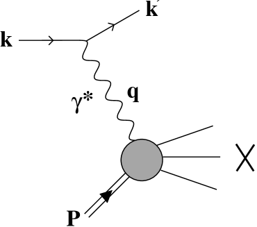
Fig. 2.1: Inclusive deep-inelastic lepton-nucleon scattering.

Neglecting weak interactions which are relevant at very high energies only, the differential cross section is given by:

$$\frac{d^{2}\sigma}{d\mathchar 10\relax dE^{\prime}}=\frac{\alpha^{2}}{Q^{4}}\frac{E^{\prime}}{E}L_{\mu\nu}W^{\mu\nu},$$ (2.1)

to leading order in the electromagnetic coupling constant $\alpha=e^{2}/4\pi\simeq 1/137$. Here

$$q^{\mu}=k^{\mu}-{k^{\prime}}^{\mu}=(\nu,\mathchoice{\mbox{\boldmath$q$}}{\mbox{\boldmath$q$}}{\kern-0.20004pt\hbox{$\scriptstyle q$}\kern-3.37604pt\kern 0.39993pt\hbox{$\scriptstyle q$}\kern-3.37604pt\kern-0.20004pt\raise 0.21698pt\hbox{$\scriptstyle q$}}{\kern-0.20004pt\hbox{$\scriptscriptstyle q$}\kern-2.41144pt\kern 0.39993pt\hbox{$\scriptscriptstyle q$}\kern-2.41144pt\kern-0.20004pt\raise 0.21698pt\hbox{$\scriptscriptstyle q$}})$$ (2.2)

is the four-momentum of the exchanged virtual photon, and $Q^{2}=-q^{2}$. The lepton-photon interaction is described by the lepton tensor $L_{\mu\nu}$. Let the spin projections of the initial and final lepton be $s$ and $s^{\prime}$. After summing over $s^{\prime}$ the lepton tensor can be split into pieces which are symmetric and antisymmetric with respect to the Lorentz indices $\mu$ and $\nu$:

$$L_{\mu\nu}(k,s;k^{\prime})=L_{\mu\nu}^{S}(k;k^{\prime})+i\,L_{\mu\nu}^{A}(k,s;k^{\prime}),$$ (2.3)

with:

$$L_{\mu\nu}^{S}(k;k^{\prime})\,=\,2\left(k_{\mu}k^{\prime}_{\nu}+k_{\nu}k^{\prime}_{\mu}\right)+g_{\mu\nu}\,q^{2},$$ (2.4)

$$L_{\mu\nu}^{A}(k,s;k^{\prime})\,=\,2\,m\,\epsilon_{\mu\nu\alpha\beta}\,s^{\alpha}\,q^{\beta},$$ (2.5)

where the lepton spin vector is defined by $2m\,s^{\alpha}=\bar{u}\gamma^{\alpha}\gamma_{5}u$. For unpolarized lepton scattering the average over the initial lepton polarization is carried out. In this case only the symmetric term, $L_{\mu\nu}^{S}$, remains.

The complete information about the target response is in the hadronic tensor $W_{\mu\nu}$. We denote the nucleon spin by $S$. Gauge invariance and symmetry properties allow a parametrization of the hadronic tensor,

$$W_{\mu\nu}(q;P,S)=W_{\mu\nu}^{S}(q;P)+i\,W_{\mu\nu}^{A}(q;P,S),$$ (2.6)

in terms of four structure functions. The symmetric part is

$$W_{\mu\nu}^{S}(q;P) = \left(\frac{q_{\mu}q_{\nu}}{q^{2}}-g_{\mu\nu}\right)W_{1}(P\cdot q,q^{2})$$ (2.7)

$$+ \left(P_{\mu}-\frac{P\cdot q}{q^{2}}q_{\mu}\right)\left(P_{\nu}-\frac{P\cdot q}{q^{2}}q_{\nu}\right)\frac{W_{2}(P\cdot q,q^{2})}{M^{2}},$$

and the antisymmetric part can be written

$$W_{\mu\nu}^{A}(q;P,S) = \epsilon_{\mu\nu\alpha\beta}\,q^{\alpha}\left[S^{\beta}MG_{1}(P\cdot q,q^{2})+\left(P\cdot q\,S^{\beta}-S\cdot q\,P^{\beta}\right)\frac{G_{2}(P\cdot q,q^{2})}{M}\right].$$

Here the nucleon spin vector $S^{\mu}$, with $2MS^{\mu}=\overline{U}(P,S)\,\gamma^{\mu}\gamma_{5}\,U(P,S)$, has been introduced. In the conventions used in this paper nucleon Dirac spinors $U$ are normalized according to $\bar{U}(P)\gamma^{\mu}U(P)=2P^{\mu}$. It is evident that $W_{1,2}$ can be measured in unpolarized scattering processes, whereas the complete investigation of $G_{1,2}$ requires both beam and target to be polarized.

It is convenient to introduce dimensionless structure functions

$$F_{1}(x,Q^{2}) = M\,W_{1}(P\cdot q,q^{2}),$$ (2.9)

$$F_{2}(x,Q^{2}) = \frac{P\cdot q}{M}\,W_{2}(P\cdot q,q^{2}),$$ (2.10)

which depend on the Bjorken scaling variable,

$$x=\frac{Q^{2}}{2P\cdot q}.$$ (2.11)

In terms of $F_{1,2}$ the charged lepton scattering cross section (2.1) for an unpolarized lepton and nucleon is:

$$\frac{d^{2}\sigma}{dx\,dQ^{2}}=\frac{4\pi\alpha^{2}}{Q^{4}}\left[\left(1-y-\frac{Mxy}{2E}\right)\frac{F_{2}}{x}+y^{2}F_{1}\right],$$ (2.12)

with

$$y=\frac{P\cdot q}{P\cdot k}.$$ (2.13)

Let us recall the behavior of the structure functions in the Bjorken limit, i.e. at large momentum and energy transfers,

$$Q^{2}=-q^{2}\rightarrow\infty,\quad P\cdot q\rightarrow\infty,$$ (2.14)

but fixed ratio $Q^{2}/P\cdot q$. Here the unpolarized structure functions

$$F_{1}(x,Q^{2}) \stackrel{{\scriptstyle Q^{2}\rightarrow\infty}}{{\relbar\joinrel\relbar\joinrel\longrightarrow}}F_{1}(x),$$ (2.15)

$$F_{2}(x,Q^{2}) \stackrel{{\scriptstyle Q^{2}\rightarrow\infty}}{{\relbar\joinrel\relbar\joinrel\longrightarrow}}F_{2}(x)$$ (2.16)

are observed to depend in good approximation only on the dimensionless Bjorken scaling variable $x$. Variations of the structure functions with $Q^{2}$ at fixed $x$ turn out to be small.

A similar scaling behavior is expected for the spin-dependent structure functions:

$$g_{1}(x,Q^{2}) = MP\cdot q\,G_{1}(P\cdot q,q^{2}),$$ (2.17)

$$g_{2}(x,Q^{2}) = \frac{(P\cdot q)^{2}}{M}\,G_{2}(P\cdot q,q^{2}),$$ (2.18)

which likewise reduce to functions of $x$ only when the limit $Q^{2}\rightarrow\infty$ is taken.

2.2 Parton model

The approximate $Q^{2}$-independence of nucleon structure functions at large $Q^{2}$ has led to the conclusion that the virtual photon sees point-like constituents in the nucleon. This is the basis of the naive parton model which gives a simple interpretation of nucleon structure functions. In this picture the nucleon is composed of free pointlike constituents, the partons, identified with quarks and gluons. Introducing distributions $q_{f}(x)$ and $\bar{q}_{f}(x)$ of quarks and antiquarks with flavor $f$ and fractional electric charge $e_{f}$, one finds:

$$F_{1}(x) = \frac{1}{2}\sum_{f}e_{f}^{2}\left(q_{f}(x)+\bar{q}_{f}(x)\right),$$ (2.19)

$$F_{2}(x) = 2x\,F_{1}(x).$$ (2.20)

The Bjorken variable $x$ coincides with the fraction of the target light-cone momentum carried by the interacting quark with momentum $l$:

$$x=\frac{Q^{2}}{2P\cdot q}=\frac{l\cdot q}{P\cdot q}.$$ (2.21)

The Callan-Gross relation (2.20) connecting $F_{1}$ and $F_{2}$ reflects the spin-$1/2$ nature of the quarks.

For the spin structure functions the naive parton model gives:

$$g_{1}(x) = \frac{1}{2}\sum_{f}e_{f}^{2}\left[\mathchar 1\relax q_{f}(x)+\mathchar 1\relax\bar{q}_{f}(x)\right],$$ (2.22)

$$g_{2}(x) = 0.$$ (2.23)

The helicity distributions $\mathchar 1\relax q_{f}(x)=q_{f}^{\uparrow}(x)-q_{f}^{\downarrow}(x)$ and $\mathchar 1\relax\bar{q}_{f}(x)=\bar{q}_{f}^{\uparrow}(x)-\bar{q}_{f}^{\downarrow}(x)$ involve the differences of quark or antiquark distributions with helicities parallel and antiparallel with respect to the helicity of the target nucleon.

2.3 Virtual Compton scattering

The hadronic tensor (2.6) can be expressed as the Fourier transform of a correlation function of electromagnetic currents, with its expectation value taken for the nucleon ground state $|P,S\rangle$ normalized as $\langle P^{\prime},S^{\prime}|P,S\rangle=2E_{{\mathrm{p}}}\,(2\pi)^{3}\,\delta^{3}(\mathchoice{\mbox{\boldmath$P$}}{\mbox{\boldmath$P$}}{\kern-0.20004pt\hbox{$\scriptstyle P$}\kern-5.46632pt\kern 0.39993pt\hbox{$\scriptstyle P$}\kern-5.46632pt\kern-0.20004pt\raise 0.21698pt\hbox{$\scriptstyle P$}}{\kern-0.20004pt\hbox{$\scriptscriptstyle P$}\kern-3.90451pt\kern 0.39993pt\hbox{$\scriptscriptstyle P$}\kern-3.90451pt\kern-0.20004pt\raise 0.21698pt\hbox{$\scriptscriptstyle P$}}-\mathchoice{\mbox{\boldmath$P$}}{\mbox{\boldmath$P$}}{\kern-0.20004pt\hbox{$\scriptstyle P$}\kern-5.46632pt\kern 0.39993pt\hbox{$\scriptstyle P$}\kern-5.46632pt\kern-0.20004pt\raise 0.21698pt\hbox{$\scriptstyle P$}}{\kern-0.20004pt\hbox{$\scriptscriptstyle P$}\kern-3.90451pt\kern 0.39993pt\hbox{$\scriptscriptstyle P$}\kern-3.90451pt\kern-0.20004pt\raise 0.21698pt\hbox{$\scriptscriptstyle P$}}^{\prime})\,\delta_{SS^{\prime}}$ [6, 7, 8]:

$$W_{\mu\nu}(q;P,S)=\frac{1}{4\pi\,M}\intop{d}^{4}z\,e^{iq\cdot z}\,\langle P,S|J_{\mu}(z)J_{\nu}(0)|P,S\rangle.$$ (2.24)

It is related to the forward virtual Compton scattering amplitude:

$$T_{\mu\nu}(q;P,S)=i\intop{d}^{4}z\,e^{iq\cdot z}\,\langle P,S|{\cal T}\left(J_{\mu}(z)J_{\nu}(0)\right)|P,S\rangle,$$ (2.25)

where ${\cal T}$ denotes the time-ordered product. By comparison of Eqs.(2.24) and (2.25) one finds the optical theorem:

$$2\pi M\,W_{\mu\nu}={{\mathrm{Im}}}\,T_{\mu\nu}.$$ (2.26)

Consequently, nucleon structure functions can be represented in terms of virtual photon-nucleon helicity amplitudes,

$${\cal A}_{hH,h^{\prime}H^{\prime}}=e^{2}\epsilon^{\mu*}_{h^{\prime}}T_{\mu\nu}(H,H^{\prime})\,\epsilon_{h}^{\nu}.$$ (2.27)

Here $\epsilon_{h}$ and $\epsilon_{h^{\prime}}$ are the polarization vectors of the incoming and scattered photon with helicities $h$ and $h^{\prime}$, respectively. They have values $+1,-1,0$ (abbreviated as $+,-,0$). Helicities of the initial and final nucleon are denoted by $H$ and $H^{\prime}$. Their values are $\pm 1$, symbolically denoted by $\uparrow,\downarrow$. Choosing the $z$-axis in space to coincide with $\mathchoice{\mbox{\boldmath$q$}}{\mbox{\boldmath$q$}}{\kern-0.20004pt\hbox{$\scriptstyle q$}\kern-3.37604pt\kern 0.39993pt\hbox{$\scriptstyle q$}\kern-3.37604pt\kern-0.20004pt\raise 0.21698pt\hbox{$\scriptstyle q$}}{\kern-0.20004pt\hbox{$\scriptscriptstyle q$}\kern-2.41144pt\kern 0.39993pt\hbox{$\scriptscriptstyle q$}\kern-2.41144pt\kern-0.20004pt\raise 0.21698pt\hbox{$\scriptscriptstyle q$}}/|\mathchoice{\mbox{\boldmath$q$}}{\mbox{\boldmath$q$}}{\kern-0.20004pt\hbox{$\scriptstyle q$}\kern-3.37604pt\kern 0.39993pt\hbox{$\scriptstyle q$}\kern-3.37604pt\kern-0.20004pt\raise 0.21698pt\hbox{$\scriptstyle q$}}{\kern-0.20004pt\hbox{$\scriptscriptstyle q$}\kern-2.41144pt\kern 0.39993pt\hbox{$\scriptscriptstyle q$}\kern-2.41144pt\kern-0.20004pt\raise 0.21698pt\hbox{$\scriptscriptstyle q$}}|$, the direction of the propagating virtual photon, and quantizing the angular momentum of the target and photon along this axis yields the following relations:

$$F_{1} = \frac{1}{4\pi e^{2}}\left({{\mathrm{Im}}}\,{\cal A}_{+\downarrow,+\downarrow}+{{\mathrm{Im}}}\,{\cal A}_{+\uparrow,+\uparrow}\right),$$ (2.28)

$$F_{2} = \frac{x}{2\pi e^{2}\kappa}\left({{\mathrm{Im}}}\,{\cal A}_{+\downarrow,+\downarrow}+{{\mathrm{Im}}}\,{\cal A}_{+\uparrow,+\uparrow}+2\,{{\mathrm{Im}}}\,{\cal A}_{0\uparrow,0\uparrow}\right),$$ (2.29)

where $\kappa=1+(2Mx/Q)^{2}$. For the spin-dependent structure functions one finds:

$$g_{1} = \frac{1}{4\pi e^{2}\kappa}\left({{\mathrm{Im}}}\,{\cal A}_{+\downarrow,+\downarrow}-{{\mathrm{Im}}}\,{\cal A}_{+\uparrow,+\uparrow}+\sqrt{2(\kappa-1)}\,{{\mathrm{Im}}}\,{\cal A}_{+\downarrow,0\uparrow}\right),$$ (2.30)

$$g_{2} = \frac{1}{4\pi e^{2}\kappa}\left({{\mathrm{Im}}}\,{\cal A}_{+\uparrow,+\uparrow}-{{\mathrm{Im}}}\,{\cal A}_{+\downarrow,+\downarrow}+\frac{2}{\sqrt{2(\kappa-1)}}\,{{\mathrm{Im}}}\,{\cal A}_{+\downarrow,0\uparrow}\right).$$ (2.31)

In the scaling limit the structure functions $F_{1}$, $F_{2}$ and $g_{1}$ are determined by helicity conserving amplitudes. It is therefore possible to express them through virtual photon-nucleon cross sections defined as:

$$\sigma_{hH}=\frac{1}{2MK}{{\mathrm{Im}}}\,{\cal A}_{hH,hH},$$ (2.32)

with the virtual photon flux $K=(2P\cdot q-Q^{2})/2M$. For example, the structure function $F_{2}$ reads:

$$F_{2}=\frac{1-x}{1+(2Mx/Q)^{2}}\frac{Q^{2}}{4\pi^{2}\alpha}\left(\sigma_{L}+\sigma_{T}\right),$$ (2.33)

where the longitudinal and transverse photon-nucleon cross sections $\sigma_{L,T}(\nu,Q^{2})$ are given by:

$$\sigma_{L} = \frac{1}{2}\left(\sigma_{0\uparrow}+\sigma_{0\downarrow}\right),$$ (2.34)

$$\sigma_{T} = \frac{1}{4}\left(\sigma_{+\uparrow}+\sigma_{+\downarrow}+\sigma_{-\uparrow}+\sigma_{-\downarrow}\right).$$ (2.35)

An interesting quantity is their ratio:

$$R=\frac{\sigma_{L}}{\sigma_{T}}=\frac{F_{2}(1+(2Mx/Q)^{2})}{2xF_{1}}-1.$$ (2.36)

In the simple parton model the Callan-Gross relation (2.20) implies $R=0$ as $Q^{2}\rightarrow\infty$. Due to their interaction with gluons, quarks receive momentum components transverse to the photon direction. Then they can absorb also longitudinally polarized photons. This leads to $R\neq 0$.

2.4 QCD-improved parton model

Nucleon structure functions systematically exhibit a weak $Q^{2}$-dependence, even at large $Q^{2}$. These scaling violations can be described within the framework of the QCD-improved parton model which incorporates the interaction between quarks and gluons in the nucleon in a perturbative way (see e.g. [6, 7, 8]). The scale at which this interaction is resolved is determined by the momentum transfer. The $Q^{2}$-dependence of parton distributions, e.g.

$$F_{2}(x,Q^{2}) = \sum_{f}e_{f}^{2}\,x\,\left[q_{f}(x,Q^{2})+\bar{q}_{f}(x,Q^{2})\right],$$ (2.37)

$$g_{1}(x,Q^{2}) = \frac{1}{2}\sum_{f}e_{f}^{2}\left[\mathchar 1\relax q_{f}(x,Q^{2})+\mathchar 1\relax\bar{q}_{f}(x,Q^{2})\right],$$ (2.38)

is described by the Dokshitzer-Gribov-Lipatov-Altarelli-Parisi (DGLAP) evolution equations. They are different for flavor non-singlet and singlet distribution functions. Typical examples of non-singlet combinations are the difference of quark and antiquark distribution functions, or the difference of up and down quark distributions. The difference of the proton and neutron structure function, $F_{2}^{{\mathrm{p}}}-F_{2}^{{\mathrm{n}}}$, also behaves as a flavor non-singlet, whereas the deuteron structure function $F_{2}^{{\mathrm{d}}}$ is an almost pure flavor singlet combination. For the flavor non-singlet quark distribution, $q^{{\mathrm{NS}}}$, and the flavor-singlet quark and gluon distributions, $q^{{\mathrm{S}}}$ and $g$, the DGLAP evolution equations read as follows:

$$\frac{{d}q^{{\mathrm{NS}}}(x,Q^{2})}{{d}\ln Q^{2}} = \frac{\alpha_{s}(Q^{2})}{2\pi}\intop_{x}^{1}\frac{{d}y}{y}q^{{\mathrm{NS}}}(y,Q^{2})P_{qq}\left(\frac{x}{y}\right),$$ (2.39)

$$\frac{d}{{d}\ln Q^{2}}\left(\begin{array}[]{c}q^{{\mathrm{S}}}(x,Q^{2})\\ g(x,Q^{2})\end{array}\right) = \frac{\alpha_{s}(Q^{2})}{2\pi}\intop_{x}^{1}\frac{{d}y}{y}\left(\begin{array}[]{rr}P_{qq}(\frac{x}{y})&P_{qg}(\frac{x}{y})\\ P_{gq}(\frac{x}{y})&P_{gg}(\frac{x}{y})\end{array}\right)\left(\begin{array}[]{c}q^{{\mathrm{S}}}(y,Q^{2})\\ g(y,Q^{2})\end{array}\right).$$ (2.46)

Here $\alpha_{s}(Q^{2})$ is the running QCD coupling strength. The splitting function $P_{qq}(x/y)$ determines the probability for a quark to radiate a gluon such that the quark momentum is reduced by a fraction $x/y$. Similar interpretations hold for the remaining splitting functions. For further details we refer the reader to one of the many textbooks on applications of QCD, e.g. [6, 7, 8].

2.5 Light-cone dominance of deep-inelastic scattering

The QCD analysis of deep-inelastic scattering has generated its own terminology and specialized jargon. In this section we summarize some of the basic notions. The general framework is Wilson’s operator product expansion applied to the current-current correlation function. A detailed investigation reveals that the hadronic tensor

$$2\pi\,M\,W_{\mu\nu}={{\mathrm{Im}}}\left[\,i\intop{d}^{4}z\,e^{iq\cdot z}\left\langle P\right|{\cal T}\left(J_{\mu}(z)J_{\nu}(0)\right)\left|P\right\rangle\right],$$ (2.47)

at $Q^{2}\rightarrow\infty$ but fixed Bjorken $x$, is dominated by contributions from near the light-cone, $z^{2}=t^{2}-\mathchoice{\mbox{\boldmath$z$}}{\mbox{\boldmath$z$}}{\kern-0.20004pt\hbox{$\scriptstyle z$}\kern-3.5632pt\kern 0.39993pt\hbox{$\scriptstyle z$}\kern-3.5632pt\kern-0.20004pt\raise 0.21698pt\hbox{$\scriptstyle z$}}{\kern-0.20004pt\hbox{$\scriptscriptstyle z$}\kern-2.54514pt\kern 0.39993pt\hbox{$\scriptscriptstyle z$}\kern-2.54514pt\kern-0.20004pt\raise 0.21698pt\hbox{$\scriptscriptstyle z$}}^{2}\simeq 0$ [6, 7, 8]. The operator product expansion makes use of this fact by expanding the time-ordered product of currents around the singularity at $z^{2}=0$:

$${\cal T}\left(J(z)J(0)\right)\sim\sum_{n=0}^{\infty}c^{\cal O}_{n}(z^{2};\mu^{2})\,z^{\mu_{1}}\cdots z^{\mu_{n}}\,{\cal O}_{\mu_{1}\cdots\mu_{n}}(\mu^{2}),$$ (2.48)

where the ${\cal O}_{\mu_{1}\cdots\mu_{n}}$ are local operators involving quark and gluon fields. The coefficient functions $c_{n}$ are singular at $z^{2}=0$. They are grouped according to the order of their singularity. Both the operators ${\cal O}$ and the c-number coefficient functions $c_{n}$ depend on the renormalization point $\mu^{2}$.

The operators ${\cal O}$ can be organized according to the irreducible representation of the Lorentz group to which they belong. Each operator has a characteristic dimensionality, $d$, in powers of mass or momentum. For example, the symmetric traceless Lorentz tensors of rank $n$ with minimum dimensionality are the operators

$${\cal O}_{\mu_{1}\cdots\mu_{n}}^{q} = \left\{\overline{\psi}\gamma_{\mu_{1}}iD_{\mu_{2}}\cdots iD_{\mu_{n}}\psi\right\}_{\cal S},$$ (2.49)

$${\cal O}_{\mu_{1}\cdots\mu_{n}}^{g} = \left\{G_{\mu_{1}\nu}iD_{\mu_{2}}\cdots iD_{\mu_{n-1}}G_{\mu_{n}}^{\nu}\right\}_{\cal S},$$ (2.50)

local bilinears in the quark field $\psi$ and the gluon field tensor $G_{\mu\nu}$, with any number of gauge-covariant derivatives $D_{\mu}$ inserted between them. The brackets $\{\}_{\cal S}$ indicate symmetrization with respect to Lorentz indices and subtraction of trace terms. The operators ${\cal O}^{q}$ and ${\cal O}^{g}$ have dimensionality $d=3+(n-1)=4+(n-2)=2+n$. The difference $\tau=d-n$ is called “twist” ($\tau=2$ in our example), a useful bookkeeping device to classify the light-cone ($z^{2}\rightarrow 0$) singularity of the coefficient function $c_{n}$. Comparing dimensions in Eq.(2.48) one finds that, for each given operator on the right-hand side, the coefficient behaves as $c_{n}\sim(1/z^{2})^{(2d_{J}-\tau)/2}$ when $z^{2}\rightarrow 0$, where $d_{J}=3$ is the dimensionality of each of the currents on the left-hand side of Eq.(2.48).

Matrix elements of the operators $\cal O$ between nucleon states are of genuinely non-perturbative origin. For spin-averaged quantities they must be of the form

$$\langle P|{\cal O}_{\mu_{1}\cdots\mu_{n}}^{q}(\mu^{2})|P\rangle = a^{q}_{n}(\mu^{2})P_{\mu_{1}}\cdots P_{\mu_{n}},$$ (2.51)

$$\langle P|{\cal O}_{\mu_{1}\cdots\mu_{n}}^{g}(\mu^{2})|P\rangle = a^{g}_{n}(\mu^{2})P_{\mu_{1}}\cdots P_{\mu_{n}},$$ (2.52)

since Lorentz-covariant tensorial functions of the nucleon four-momentum $P^{\mu}$, with $P^{2}=M^{2}$ fixed, are proportional to the symmetric tensors $P_{\mu_{1}}\cdots P_{\mu_{n}}$. Trace terms have been subtracted in Eqs.(2.51,2.52). The constants $a_{n}^{q}$ and $a_{n}^{g}$ are fixed at a given renormalization scale $\mu^{2}$ and represent the non-perturbative quark and gluon dynamics of the nucleon.

We can now make contact with observables. Since the Fourier transform of $\langle P|T(J_{\mu}(z)J_{\nu}(0)|P\rangle$ is proportional to the forward virtual Compton scattering amplitude and its imaginary part determines the structure functions $F_{1}$ and $F_{2}$, it is clear that the $a_{n}$ represent moments of those structure functions, with $Q^{2}$-dependent coefficients. Consider as an example the structure function $F_{1}(x,Q^{2})$ in the flavor singlet channel. One finds,

$$\intop_{0}^{1}{d}x\,x^{n-1}F_{1}(x,Q^{2})=C_{n}^{q}(Q^{2};\mu^{2})\,a^{q}_{n}(\mu^{2})+C_{n}^{g}(Q^{2};\mu^{2})\,a^{g}_{n}(\mu^{2}),$$ (2.53)

where crossing symmetry implies a restriction to even orders $n=2,4,\dots$. The momentum space coefficient functions $C_{n}(Q^{2};\mu^{2})$ are related to the c-number functions $c_{n}(z^{2};\mu^{2})$ of Eq.(2.48) by Fourier transformation. The important point is that the $C_{n}(Q^{2};\mu^{2})$ can be calculated perturbatively at large $Q^{2}$. Their $Q^{2}$-dependence is determined by renormalization group equations equivalent to the DGLAP equations in (2.46).

It is often useful to express the structure functions in a factorized form, by a convolution of “hard” effective cross sections $\hat{\sigma}_{q}$ and $\hat{\sigma}_{g}$ for the scattering of the virtual photon from quarks and gluons in the nucleon, with “soft” quark and gluon distributions of the target. For example,

$$F_{1}(x,Q^{2}) = \intop_{x}^{1}\frac{{d}y}{y}\,\left\{\hat{\sigma}_{q}(y,Q^{2};\mu^{2})\,\left[q(x/y,\mu^{2})+\bar{q}(x/y,\mu^{2})\right]\right.$$ (2.54)

$$\hskip 56.9055pt+\left.\hat{\sigma}_{g}(y,Q^{2};\mu^{2})\,g(x/y,\mu^{2})\right\}.$$

(Here we have generically used only one quark flavor with unit electric charge.) The perturbatively calculable functions $C_{n}$ then find a simple physical interpretation in terms of moments of the “hard” cross sections:

$$C^{q,g}_{n}(Q^{2};\mu^{2})=\intop_{0}^{1}{d}x\,x^{n-1}\hat{\sigma}_{q,g}(x,Q^{2};\mu^{2}),$$ (2.55)

while the quark and gluon distributions are related to the “soft” reduced matrix elements (2.51,2.52) by

$$a^{q}_{n}(\mu^{2}) = \intop_{0}^{1}{d}x\,x^{n-1}\left[q(x,\mu^{2})+(-1)^{n}{\bar{q}}(x,\mu^{2})\right],$$ (2.56)

$$a^{g}_{n}(\mu^{2}) = \intop_{0}^{1}dx\,x^{n-1}g(x,\mu^{2}),$$ (2.57)

where Eq.(2.57) holds only for even $n$. To lowest (zeroth) order in the running coupling strength $\alpha_{s}(\mu^{2})$, the “hard” cross sections are simply $\hat{\sigma}_{q}\sim\delta(1-x)$ and $\hat{\sigma}_{g}=0$, so that only quarks contribute to $F_{1}$. Gluons first enter at order $\alpha_{s}$. We mention that, in general, the representation of a given structure function in terms of separate quark and gluon contributions is a matter of definition. It is unique only in leading order and depends on the renormalization scheme at higher orders in $\alpha_{s}$ [6, 7, 8]. The measured structure functions are, of course, free of such ambiguities.

2.6 Facts about free nucleon structure functions

In this section we briefly review the present experimental status on free nucleon structure functions as measured in deep-inelastic lepton scattering. We focus on those aspects which are of direct relevance for our further discussion of nuclear deep-inelastic scattering.

2.6.1 Spin independent structure functions

Unpolarized deep-inelastic scattering has been explored in recent years over a wide kinematic range in fixed target experiments at CERN, FNAL and SLAC, and at the HERA collider at DESY. Reviews can be found e.g. in Refs.[9, 10, 11].

The proton structure function $F_{2}^{{\mathrm{p}}}$

Accurate $F_{2}^{{\mathrm{p}}}$ data are available from fixed target measurements at SLAC, at CERN (BCDMS, NMC) and at Fermilab (E665). They cover the kinematic range $10^{-3}<x<0.8$ and $0.2\,{{\mathrm{GeV}}}^{2}<Q^{2}<260$ GeV² [9]. Due to experimental constraints fixed target studies at small $x$ are possible only at low $Q^{2}$. For example, in the E665 measurements at Fermilab the smallest values of the Bjorken variable, $x\simeq 0.8\cdot 10^{-3}$, are measured typically at $Q^{2}\simeq 0.2$ GeV² [12]. This is different at the HERA collider where the kinematic range $3\cdot 10^{-6}<x<0.5$ and $0.16\,{{\mathrm{GeV}}}^{2}<Q^{2}<5000$ GeV² is explored. In these experiments the region of small $x$ is accessible also at large $Q^{2}$.

The data summarized in Figures 2.2 and 2.3 display several important features (for references see e.g. [9, 10, 11]):

Fig. 2.2: The proton structure function $F_{2}^{{\mathrm{p}}}$ as a function of $x$ for various $Q^{2}$. The data are taken from H1 [13, 14], ZEUS [15, 16, 17], E665 [12], NMC [18], SLAC [19], and BCDMS [20].

Fig. 2.3: The $Q^{2}$-dependence of the proton structure function $F_{2}^{{\mathrm{p}}}$ for $x<0.1$. The data are taken from ZEUS [16, 17], E665 [12], and NMC [18].

• At small Bjorken-$x$ ($x\ll 0.1$) but large $Q^{2}$ a strong increase of $F_{2}^{{\mathrm{p}}}$ with decreasing $x$ has been found at HERA. This behavior is commonly interpreted in terms of the dominant role of gluons at small $x$, the density of which rises strongly with decreasing $x$. This increase becomes weaker at low $Q^{2}$. Here only a minor $x$-dependence has been observed in fixed target experiments, which is nevertheless enhanced at very small $x\ll 0.1$ as recently explored at HERA [14, 17]. Note that a rise of $F_{2}^{{\mathrm{p}}}$ with decreasing $x$ reflects a growing virtual photon-proton cross section as the photon-nucleon center-of-mass energy $W=\sqrt{s}$ increases. For example, at $Q^{2}\simeq 100$ GeV² one observes a characteristic behavior [13]:

  $$\sigma_{\gamma^{*}{{\mathrm{p}}}}\sim\left(W^{2}\right)^{\mathchar 1\relax},\quad\mbox{with}\,\mathchar 1\relax\approx 0.3.$$ (2.58)

  For the real photon-nucleon cross section at high energies, on the other hand, one has $\mathchar 1\relax\approx 0.08$ [21]. The dynamical origin of the observed variation of the energy dependence of $\sigma_{\gamma^{*}{\mathrm{N}}}$ with $Q^{2}$ is an important issue of ongoing investigations (see for example Refs.[9, 10]).

  Hadron-hadron interaction cross sections have an energy dependence similar to that observed in photon-nucleon scattering. It is often parametrized using Regge phenomenology [21, 22]. In Regge theory the dependence of cross sections on the center-of-mass energy is determined by the $t$-channel exchange of families of particles permitted by the conservation of all relevant quantum numbers. Each group of particles is characterized by a Regge trajectory, $\alpha(t)\approx\alpha(0)+t\,\alpha^{\prime}$, which relates their spin with their invariant mass. The resulting dependence of hadron-hadron total cross sections on the squared center-of-mass energy $s$ is:

  $$\sigma_{tot}\sim s^{\alpha(0)-1}.$$ (2.59)

  The rising hadron-hadron cross sections at high energies are well described by the so-called pomeron exchange. It corresponds to multi-gluon exchange with vacuum quantum numbers and it is characterized by the trajectory [21, 23]

  $$\alpha_{{}_{\rm I\!P}}(t)\approx\alpha_{{}_{\rm I\!P}}(0)+t\,\alpha_{{}_{\rm I\!P}}^{\prime}\approx 1.08+t\,0.26\,\mbox{GeV}^{-2}\,.$$ (2.60)

  Note that the fast growth of the interaction cross section (2.59) with energy as implied by Eq.(2.60) cannot persist up to arbitrarily high energies because of limitations imposed by unitarity. At asymptotic energies the Froissart bound does not permit total hadronic cross sections to rise faster than $(\ln s/s_{0})^{2}$ with some constant scale $s_{0}$ [22].

  The slow decrease of hadron cross sections at moderate energies is described by an exchange made up from a set of reggeons which lie on the approximately degenerate trajectory [21, 24]

  $$\alpha_{{}_{\rm I\!R}}(t)\approx\alpha_{{}_{\rm I\!R}}(0)+t\,\alpha_{{}_{\rm I\!R}}^{\prime}\approx 0.5+t\,0.9\,\mbox{GeV}^{-2}\,,$$ (2.61)

  and which carry the quantum numbers of the $\rho,\omega,a_{2}$ and $f_{2}$ mesons, respectively. At large energies these so-called subleading contributions are exceeded by pomeron exchange (2.60).

• At small values of $Q^{2}$ (i.e. $Q^{2}<1$ GeV²) the structure function $F_{2}^{{\mathrm{p}}}$ drops. This is quite natural in view of the fact that $F_{2}^{{\mathrm{p}}}$ has to vanish linearly with $Q^{2}$ in the limit $Q^{2}\rightarrow 0$ as a consequence of current conservation (see e.g. [11]). Bjorken scaling must break down in this kinematic regime. In particular, at small $x<0.1$ or large photon energy, $\nu>5$ GeV, vector meson dominance is expected to play an important role. It describes (virtual) photon-nucleon scattering via the interaction of vector meson fluctuations of the photon. The contribution to $F_{2}^{{\mathrm{p}}}$ from the three lightest vector mesons reads (see e.g. [25]):

  $$F_{2}^{{{\mathrm{p}}}(VMD)}(x,Q^{2})=\frac{Q^{2}}{4\pi}\sum_{{\mathrm{V}}={\rho,\omega,\phi}}\left(\frac{m_{\mathrm{V}}^{2}}{g_{{\mathrm{V}}}}\right)^{2}\left(\frac{1}{m_{{\mathrm{V}}}^{2}+Q^{2}}\right)^{2}\sigma_{{\mathrm{Vp}}}.$$ (2.62)

  The sum is taken over $\rho$, $\omega$, and $\phi$ mesons with their invariant masses $m_{\mathrm{V}}$. The vector meson-proton cross sections are denoted by $\sigma_{{\mathrm{Vp}}}$. The vector meson-photon coupling constants $g_{{\mathrm{V}}}$ can be deduced from electron-positron annihilation into those vector mesons. One observes that $F_{2}^{{{\mathrm{p}}}(VMD)}\sim Q^{2}$ at small $Q^{2}$. At large $Q^{2}$, however, the vector meson contribution (2.62) vanishes as $1/Q^{2}$. Then the scattering from parton constituents in the target takes over and leads to Bjorken scaling.

• Finally, at large values of $x$ one observes a rapid decrease of the structure function. This can be understood within the framework of perturbative QCD. In the limit $x\rightarrow 1$, a single valence quark struck by the virtual photon carries all of the nucleon momentum. The only way for such a configuration to evolve from a bound state wave function which is centered around low parton momenta, is through the exchange of hard gluons. A perturbative description of this process leads to $F_{2}^{{{\mathrm{p}}}}(x\rightarrow 1)\sim(1-x)^{3}$ [26].

2.6.2 The ratio of longitudinal and transverse cross sections

Extracting the structure function $F_{2}$ from lepton scattering data requires information on the ratio of the total cross section for longitudinally and transversely polarized photons, $R=\frac{\sigma_{L}}{\sigma_{T}}$ from Eq.(2.36). Previous data from SLAC and CERN cover the region $0.1<x<0.9$ and $0.6\,{{\mathrm{GeV}}}^{2}<Q^{2}<80\,{{\mathrm{GeV}}^{2}}$ [27]. In this region $R$ is small. New data from the NMC collaboration are available for $0.002<x<0.12$ [18]. A rise of $R$ with decreasing $x$ has been observed as shown in Fig.2.4. This behavior can be understood within the framework of perturbative QCD [31]. Helicity conservation implies that a high-$Q^{2}$ longitudinally polarized photon cannot be absorbed by a quark moving in longitudinal direction: a non-zero transverse momentum is necessary for this process to occur. In the QCD-improved parton model such transverse quark momenta result from gluon bremsstrahlung which is important for low parton momenta, i.e. at small $x$. Further studies of $R$ in the domain of small $x$ are currently performed at HERA. A first analysis gives $R\simeq 0.5$ at $x=2.4\cdot 10^{-4}$ and $Q^{2}=15$ GeV² [32].

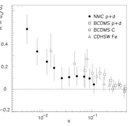
Fig. 2.4: The ratio $R=\sigma_{L}/\sigma_{T}$ as a function of $x$. The data are taken from NMC [18], BCDMS [20, 28, 29], and CDHSW [30].

2.6.3 Spin dependent structure functions

In recent years polarized deep-inelastic scattering experiments have become a major activity at all high-energy lepton beam facilities. They aim primarily at the exploration of the spin structure of nucleons. Detailed investigations have been carried out at CERN (SMC), SLAC (E142/143/154/155) and DESY (HERMES). For references see [33 – 41].

While the proton spin structure functions $g_{1}^{{\mathrm{p}}}$ and $g_{2}^{{\mathrm{p}}}$ have been measured directly using hydrogen targets, neutron structure functions have been extracted from measurements using deuterons and ${}^{3}{\mathrm{He}}$ targets with corrections for nuclear effects. In the data analysis such corrections have commonly been done in terms of effective proton and neutron polarizations obtained from realistic deuteron and ³He wave functions. They account for the fact that bound nucleons carry orbital angular momenta. As a consequence their polarization vectors need not be aligned with the total polarization of the target. At the present level of accuracy the use of effective polarizations turns out to be a reasonable approximation as discussed at length in Section 7.

In Fig.2.5 we show a collection of data for $g_{1}$. The behavior of the proton, deuteron and neutron structure functions turns out to be quite different, especially in the region of small $x$. This is in contrast to the unpolarized case where proton and neutron structure functions show a qualitatively similar behavior.

Fig. 2.5: A compilation of data of the proton, deuteron, and neutron spin structure functions $g_{1}$ from Refs.[33, 36, 37, 38, 40, 42, 43]. (We thank U. Stoesslein for the preparation of this figure.)

The moments

$$\mathchar 0\relax_{1}^{{\mathrm{p,n}}}(Q^{2})\equiv\intop_{0}^{1}{d}x\,g_{1}^{{\mathrm{p,n}}}(x,Q^{2})$$ (2.63)

of the proton and neutron spin structure functions are of fundamental importance. They can be decomposed in terms of proton matrix elements of SU$(3)$ axial currents, as follows (for a review see e.g. [44, 45]):

$$\mathchar 0\relax_{1}^{{\mathrm{p,n}}}=\frac{1}{12}\left(\frac{4}{3}\mathchar 1\relax q_{0}+\frac{1}{\sqrt{3}}\mathchar 1\relax q_{8}\pm\mathchar 1\relax q_{3}\right),$$ (2.64)

with the axial vector matrix elements:

$$MS_{\mu}\mathchar 1\relax q_{a}=\langle P,S|\bar{\psi}\gamma_{\mu}\gamma_{5}\frac{\lambda_{a}}{2}\,\psi|P,S\rangle,$$ (2.65)

where $\psi=\left(\psi_{u},\psi_{d},\psi_{s}\right)$ is the quark field. Here $\lambda_{a}$ $(a=1,\dots,8)$ denote SU$(3)$ flavor matrices and the singlet $\lambda_{0}$ is the $3\times 3$ unit matrix. In Eq.(2.64) and below we suppress QCD corrections which are currently known up to order $\alpha_{s}^{3}$. Current algebra and isospin symmetry equate the non-singlet matrix element $\mathchar 1\relax q_{3}=\mathchar 1\relax u-\mathchar 1\relax d$ with the axial vector coupling constant $g_{A}=1.26$ measured in neutron $\beta$-decay. One thus arrives at the fundamental Bjorken sum rule:

$$\mathchar 0\relax_{1}^{{\mathrm{p}}}-\mathchar 0\relax_{1}^{{\mathrm{n}}}=\frac{1}{6}\mathchar 1\relax q_{3}=\frac{1}{6}g_{A}.$$ (2.66)

Furthermore, assuming SU$(3)$ flavor symmetry, $\mathchar 1\relax q_{8}=(\mathchar 1\relax u+\mathchar 1\relax d-2\mathchar 1\relax s)/\sqrt{3}$ is determined by hyperon $\beta$-decays. The non-singlet matrix elements $\mathchar 1\relax q_{3,8}$ involve conserved currents, hence they are scale independent. This is different for the singlet term $\mathchar 1\relax q_{0}=\mathchar 1\relax u+\mathchar 1\relax d+\mathchar 1\relax s$ which receives a $Q^{2}$-dependence through the QCD axial anomaly. Note that in next-to-leading order both quarks and gluons contribute to $\mathchar 1\relax q_{0}$. However, the detailed separation into quark and gluon parts depends on the factorization scheme used to separate perturbative and non-perturbative parts of the spin-dependent cross section.

An evaluation of the structure function moments $\mathchar 0\relax_{1}^{{\mathrm{p,n}}}(Q^{2})$ from Eq.(2.63) requires knowledge of $g_{1}$ in the entire interval $0\leq x\leq 1$. Since measurements cover only a limited kinematic range, data for $g_{1}$ have to be extrapolated to $x\rightarrow 0$ and $x\rightarrow 1$. The large-$x$ extrapolation is not critical since $g_{1}$ becomes small and ultimately vanishes as $x\rightarrow 1$. The situation at small $x$ is, however, not yet well understood (for a review and references see Ref.[10]). The common approach is to assume Regge behavior which implies that $g_{1}\sim x^{\alpha}$ with $0\leq\alpha\leq 0.5$ for $x\rightarrow 0$.

A status review of the analysis of spin structure functions and their moments can be found in Refs.[34, 40]. All current studies arrive at the conclusion that the flavor singlet contribution to the nucleon spin is small. At $Q^{2}=1$ GeV² one finds (in the AB scheme) [34]:

$$\mathchar 1\relax q_{0}=0.23\pm 0.07({\mathrm{stat}})\pm 0.19({\mathrm{sys}}).$$ (2.67)

This would imply that only about one third of the nucleon spin is carried by the quark spins alone. The missing two thirds probably involve gluon spin contributions and orbital angular momentum of quark, antiquark and gluon constituents. Finally we note that the Bjorken sum rule (2.66), with inclusion of QCD corrections, is fulfilled at the $5\%$ level [34].

Measurements of $g_{2}$ have been performed at CERN [46] and SLAC [35, 47]. For the neutron case ${}^{3}{\mathrm{He}}$ [35] and deuteron [47] targets have been used again. Within large experimental errors the data for $g_{2}$ are consistent with the twist-$2$ prediction $g_{2}(x,Q^{2})=\intop_{x}^{1}\frac{dy}{y}\left(1-\delta(1-x/y)\right)g_{1}(y,Q^{2})$ of Ref.[48].

2.6.4 Diffraction

A subclass of photon-nucleon processes, namely diffractive lepto- and photoproduction, plays a prominent role also in the interaction of real and virtual photons with complex nuclei at high energies. We focus here on so-called single diffractive processes. They are characterized by the proton emerging intact and well separated in rapidity from the hadronic state $X$ produced in the dissociation of the (virtual) photon (see Fig.2.6):

$$\gamma^{(*)}+{{\mathrm{p}}}\rightarrow{{\mathrm{X}}}+{{\mathrm{p}}}^{\prime}.$$ (2.68)

As in diffractive hadron-hadron collisions such processes are important at small momentum transfer. Their cross sections drop exponentially with the squared four-momentum transfered by the colliding particles. Furthermore, they generally exhibit a weak energy dependence.

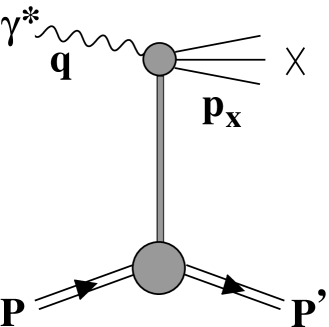
Fig. 2.6: Diffractive scattering from a nucleon.

Diffractive leptoproduction

In deep-inelastic scattering experiments at HERA approximately $10\%$ of the (virtual) photon-proton cross section result from diffractive events (for a review see e.g. [49]). Their cross section is parametrized in terms of two structure functions, analogous to the inclusive case. One has:

$$\frac{d\sigma}{dxdQ^{2}dx_{{}_{\rm I\!P}}dt}=\frac{4\pi\alpha^{2}}{Q^{4}}\left\{\frac{1-y}{x}+\frac{y^{2}}{2x\left[1+R^{{\mathrm{D}}(4)}(x,Q^{2};x_{{}_{\rm I\!P}},t)\right]}\right\}\,F_{2}^{{\mathrm{D}}(4)}(x,Q^{2};x_{{}_{\rm I\!P}},t).$$ (2.69)

The diffractive structure functions depend on $x$ and $Q^{2}$, on the squared momentum transfer $t$ to the proton, $t=(P-P^{\prime})^{2}=(q-p_{{\mathrm{X}}})^{2}$, and on the variable

$$x_{{}_{\rm I\!P}}=\frac{(P-P^{\prime})\cdot q}{P\cdot q}=\frac{Q^{2}+M_{{\mathrm{X}}}^{2}-t}{Q^{2}+W^{2}-M^{2}}\approx\frac{Q^{2}+M_{{\mathrm{X}}}^{2}}{Q^{2}+W^{2}}.$$ (2.70)

Here $M_{{\mathrm{X}}}$ is the invariant mass of the diffractively produced system ${\mathrm{X}}$ in the final state. The diffractive structure function, conventionally denoted by $F_{2}^{D(4)}$ indicating its dependence on four kinematic variables, is directly related to the diffractive (virtual) photoproduction cross section. At small $x$ one finds in analogy with Eq.(2.33):

$$F_{2}^{{\mathrm{D}}(4)}(x,Q^{2};x_{{}_{\rm I\!P}},t)\approx\frac{Q^{2}}{4\pi^{2}\alpha}\,\frac{d\sigma_{\gamma^{*}{\mathrm{p}}}^{{\mathrm{d}}iff}}{dx_{{}_{\rm I\!P}}dt}.$$ (2.71)

Most of the data have so far been obtained for the $t$-integrated structure function

$$F_{2}^{{{\mathrm{D}}}(3)}(x,Q^{2};x_{{}_{\rm I\!P}})=\intop_{-\infty}^{0}dt\,F_{2}^{{{\mathrm{D}}}(4)}(x,Q^{2};x_{{}_{\rm I\!P}},t).$$ (2.72)

Measurements by the H1 [50, 51] and ZEUS [52, 53, 54, 55] groups cover the range $4.5<Q^{2}<140$ GeV², $2\cdot 10^{-4}<x_{{}_{\rm I\!P}}<0.04$ and $0.02<x/x_{{}_{\rm I\!P}}<0.9$. No substantial $Q^{2}$-dependence of $F_{2}^{{{\mathrm{D}}}(3)}$ has been found. Over most of the explored kinematic region, $x_{{}_{\rm I\!P}}F_{2}^{{{\mathrm{D}}}(3)}$ is either decreasing or approximately constant as a function of increasing $x_{{}_{\rm I\!P}}$. However at small $x/x_{{}_{\rm I\!P}}$ there is a tendency for $x_{{}_{\rm I\!P}}F_{2}^{{{\mathrm{D}}}(3)}$ to increase at the highest values of $x_{{}_{\rm I\!P}}$. A typical collection of data is shown in Fig.2.7.

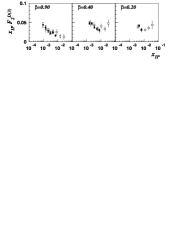
Fig. 2.7: The diffractive structure function $x_{{}_{\rm I\!P}}F_{2}^{D(3)}$ for different values of $\beta=x_{{}_{\rm I\!P}}/x$ and ${Q^{2}}\approx 28$ GeV². Data from H1 [50] (open squares) and ZEUS [52] (solid points).

A reasonably successful description of this behavior has been achieved within Regge phenomenology which assumes that the interaction proceeds in two steps: the emission of a pomeron or subleading reggeon from the proton, and the subsequent hard scattering of the virtual photon from the partons in the pomeron or reggeon, respectively. This picture leads to a factorization of the diffractive structure function [56]:

$$F_{2}^{{{\mathrm{D}}}(4)}(x,Q^{2};x_{{}_{\rm I\!P}},t)=f_{{}_{\rm I\!P}}(x_{{}_{\rm I\!P}},t)\,F_{2}^{{}^{\rm I\!P}}(x/x_{{}_{\rm I\!P}},Q^{2})+f_{{}_{\rm I\!R}}(x_{{}_{\rm I\!P}},t)\,F_{2}^{{}^{\rm I\!R}}(x/x_{{}_{\rm I\!P}},Q^{2}),$$ (2.73)

where $F_{2}^{{}^{\rm I\!P(\rm I\!R)}}$ is commonly interpreted as the “structure function” of the pomeron (reggeon) and

$$f_{i}(x_{{}_{\rm I\!P}},t)=\frac{e^{B_{i}\,t}}{x_{{}_{\rm I\!P}}^{2\alpha_{i}(t)-1}},$$ (2.74)

with $i=\rm I\!P,\rm I\!R$, denotes the pomeron (reggeon) distribution in the proton.

The H1 analysis [50] gives $\alpha_{{}_{\rm I\!P}}(0)\approx 1.2$ and $\alpha_{{}_{\rm I\!R}}(0)\approx 0.5$. The slope parameters $B_{{}_{\rm I\!P(\rm I\!R)}}$, $\alpha_{{}_{\rm I\!R}}^{\prime}$ and $\alpha_{{}_{\rm I\!P}}^{\prime}$ were taken to reproduce hadron-hadron data. While $\alpha_{{}_{\rm I\!P}}(0)$ is found to be slightly larger than the value obtained from parametrizations of hadronic cross sections, $\alpha_{{}_{\rm I\!R}}(0)$ agrees well with the Regge phenomenology of hadron–hadron collisions [21] .

In Fig.(2.8) we show recent ZEUS data [52] on the ratio of diffractive and total photon-nucleon cross sections for different regions of $M_{{\mathrm{X}}}$. The data show a similar energy dependence of both total and diffractive cross sections. Furthermore, the observed $Q^{2}$-dependence of the cross section ratio for different regions of $M_{{\mathrm{X}}}$ suggests that, as $Q^{2}$ increases, diffractive states with large mass become important.

ZEUS measurements [53] have investigated the $t$-dependence of the diffractive leptoproduction cross section. In the range $5<Q^{2}<20$ GeV² and $50<W<270$ GeV the $t$-dependence of the diffractive virtual photoproduction cross section is described for $0.07<|t|<0.4$ GeV² by the exponential form, $d\sigma_{\gamma^{*}p}^{diff}/dt\sim e^{B\,t}$, with $B\approx 7$ GeV². This value is compatible with results from high-energy hadron-hadron scattering (see e.g. [57]).

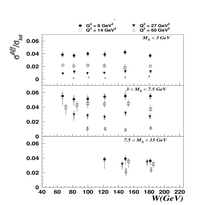
Fig. 2.8: ZEUS data [52] for the ratio of diffractive and total photon-nucleon cross sections. The diffractive production cross section has been integrated over different intervals of $M_{{\mathrm{X}}}$.

Diffractive photoproduction

Diffractive dissociation of real photons, $\gamma+{{\mathrm{N}}}\rightarrow{{\mathrm{X}}}+{{\mathrm{N}}}$, has been explored with fixed target and collider experiments. At FNAL [58] photon-proton center of mass energies up to $W\simeq 15$ GeV were used to produce diffractive states with an invariant mass up to $M_{{\mathrm{X}}}\simeq 5$ GeV. Recent experiments at HERA [59, 60, 61, 62, 63] were carried out at $W\simeq 200$ GeV and $M_{{\mathrm{X}}}<30$ GeV. The diffractive cross section amounts to approximately $20\%$ of the total photon-proton cross section. Around half of these events come from the production of the light vector mesons $\rho,\omega$ and $\phi$. This is contrary to diffractive leptoproduction at large $Q^{2}$ where vector meson contributions are suppressed roughly as $1/Q^{4}$ [64].

At sufficiently large mass $M_{{\mathrm{X}}}$ of the diffractively produced system ${\mathrm{X}}$, the measured cross sections drop approximately as $1/M_{{\mathrm{X}}}^{2}$, as shown in Fig.2.9. This is in accordance with Regge phenomenology. In the limit $W^{2}/M_{{\mathrm{X}}}^{2}\rightarrow\infty$ with $M_{{\mathrm{X}}}^{2}\rightarrow\infty$ only pomeron exchange is important and leads to [65]:

$$\frac{d\sigma_{\gamma{\mathrm{N}}}^{diff}}{dM_{{\mathrm{X}}}^{2}dt}\sim\frac{W^{4(\alpha_{{}_{\rm I\!P}}(0)-1)}}{M_{{\mathrm{X}}}^{2\alpha_{{}_{\rm I\!P}}(0)}}\,\exp\left[t\cdot\left({B+2\alpha_{{}_{\rm I\!P}}^{\prime}\ln\left(\frac{W^{2}}{M_{{\mathrm{X}}}^{2}}\right)}\right)\right],$$ (2.75)

with a slope parameter $B$. Equation (2.75) implies that at energies $W=(15-30)$ GeV typical for fixed target experiments at CERN and FNAL, the relative amount of diffraction in deep-inelastic scattering is reduced to $(10-15)\%$ [66]. Observed deviations from the simple behavior (2.75) have been associated with contributions involving subleading Regge trajectories [60, 61].

Fig. 2.9: Differential cross section for diffractive photoproduction off nucleons from FNAL [58] and H1 [61] for different center of mass energies $W$. The curves corresponds to a Regge fit [61].

3 Deep-inelastic scattering from nuclear systems

3.1 Introduction and motivation

We now enter into the central topic of this review: an exploration of new phenomena specific to deep-inelastic lepton scattering from nuclear (rather than free nucleon) targets.

Nuclei represent systems with a natural, built-in length scale. The baryon density in the center of a typical heavy nucleus is $\rho_{0}\simeq 0.15$ fm^-3. The average distance between two nucleons at this density is

$$d\simeq 1.9\,{{\mathrm{fm}}}.$$ (3.1)

The nucleons have a momentum distribution characterized by their Fermi momentum,

$$p_{F}=\left(\frac{3\pi^{2}}{2}\,\rho_{0}\right)^{1/3}\simeq 1.3\,{\mathrm{fm}}^{-1}\simeq 0.26\,{\mathrm{GeV}}.$$ (3.2)

A high energy virtual photon which scatters from this system can expect to see two sorts of genuine nuclear effects:

1. Incoherent scattering from $A$ nucleons, but with their structure functions modified in the presence of the nuclear medium. Such modifications are expected to arise, for example, from the mean field that a nucleon experiences in the presence of other nucleons, and from its Fermi motion inside the nucleus;

2. Coherent scattering processes involving more than one nucleon at a time. Such effects can occur when hadronic excitations (or fluctuations) produced by the high energy photon propagate over distances (in the laboratory frame) which are comparable to or larger than the characteristic length scale $d\sim 2$ fm of Eq.(3.1). A typical example of a coherence effect is shadowing.

It turns out, as we will demonstrate, that incoherent scattering takes place primarily in the range $0.1<x<1$ of the Bjorken variable. Strong coherence effects are observed at $x<0.1$. Cooperative phenomena in which several nucleons participate can also occur at $x>1$. (In fact, the Bjorken variable can extend, in principle, up to $x\leq A$ in a nucleus with $A$ nucleons.)

The aim of this section is to prepare the facts and phenomenology of nuclear DIS. An important subtopic in this context deals with the deuteron. While this is not a typical nucleus, it serves two purposes: first, as a convenient neutron target, and secondly, as the simplest prototype system in which coherence effects, involving proton and neutron simultaneously, can be investigated quite accurately. For this purpose we need to introduce the hadronic tensor and structure functions for spin-$1$ targets as well. Once the nuclear structure functions are at hand we will present a survey of nuclear DIS data and give first, qualitative interpretations. The more detailed understanding is then developed in subsequent sections.

3.2 Nuclear structure functions

The deep-inelastic scattering cross sections for free nucleons and nuclei have basically the same form as given by Eq.(2.1). All information about the target and its response to the interaction is included in the corresponding hadronic tensor. For nuclei with spin $1/2$ the hadronic tensor formally coincides with the one for free nucleons given in Eqs.(2.6,2.7,2.1). In this case nuclei are characterized by four structure functions, $F_{1,2}^{{\mathrm{A}}}$ and $g_{1,2}^{{\mathrm{A}}}$. For spin-$0$ targets, only the symmetric tensor (2.7) with the structure functions $F_{1,2}^{{\mathrm{A}}}$ is present. In the case of spin-$1$ targets the situation is more complex. Here the hadronic tensor is composed of eight independent structure functions [67, 68]:

$$M_{{\mathrm{A}}}\,W^{{\mathrm{A}}}_{\mu\nu} = -g_{\mu\nu}\,F_{1}^{{\mathrm{A}}}+\frac{P_{\mu}P_{\nu}}{P\cdot q}\,F_{2}^{{\mathrm{A}}}+i\frac{M_{{\mathrm{A}}}}{P\cdot q}\,\varepsilon_{\mu\nu\alpha\beta}\,q^{\alpha}\left(S^{\beta}\,(g_{1}^{{\mathrm{A}}}+g_{2}^{{\mathrm{A}}})-\frac{S\cdot q}{P\cdot q}\,P^{\beta}\,g_{2}^{{\mathrm{A}}}\right)$$ (3.3)

$$+ r_{\mu\nu}\,b_{1}^{{\mathrm{A}}}+s_{\mu\nu}\,b_{2}^{{\mathrm{A}}}+t_{\mu\nu}\,\mathchar 1\relax^{{\mathrm{A}}}+u_{\mu\nu}\,b_{3}^{{\mathrm{A}}},$$

with the Lorentz tensors:

$$r_{\mu\nu} = -g_{\mu\nu}\left(\frac{M_{{\mathrm{A}}}^{2}}{\kappa_{{\mathrm{A}}}(P\cdot q)^{2}}\,q\cdot{\cal E}\,q\cdot{\cal E}^{*}-\frac{1}{3}\right),$$ (3.4)

$$s_{\mu\nu} = \frac{P_{\mu}P_{\nu}}{P\cdot q}\left(\frac{M_{{\mathrm{A}}}^{2}}{\kappa_{{\mathrm{A}}}(P\cdot q)^{2}}\,q\cdot{\cal E}\,q\cdot{\cal E}^{*}-\frac{1}{3}\right),$$

$$t_{\mu\nu} = \frac{1}{2}\left\{\left(-g_{\mu\nu}+\frac{2x_{{\mathrm{A}}}}{\kappa_{{\mathrm{A}}}\,P\cdot q}P_{\mu}P_{\nu}\right)\left(\frac{M_{{\mathrm{A}}}^{2}}{\kappa_{{\mathrm{A}}}\,(P\cdot q)^{2}}\,q\cdot{\cal E}\,q\cdot{\cal E}^{*}-1\right)\right.$$

$$+ \left.\left[\left({\cal E}_{\mu}-\frac{q\cdot{\cal E}}{\kappa_{{\mathrm{A}}}\,P\cdot q}P_{\mu}\right)\left({\cal E}^{*}_{\nu}-\frac{q\cdot{\cal E}^{*}}{\kappa_{{\mathrm{A}}}\,P\cdot q}P_{\nu}\right)+(\mu\leftrightarrow\nu)\right]\right\},$$

$$u_{\mu\nu} = \frac{\kappa_{{\mathrm{A}}}-1}{\sqrt{\kappa_{{\mathrm{A}}}}\,P\cdot q}\left[P_{\mu}\,q\cdot{\cal E}^{*}\left({\cal E}_{\nu}-\frac{q\cdot{\cal E}}{\kappa_{{\mathrm{A}}}\,P\cdot q}P_{\nu}\right)+P_{\mu}\,q\cdot{\cal E}\left({\cal E}^{*}_{\nu}-\frac{q\cdot{\cal E}^{*}}{\kappa_{{\mathrm{A}}}\,P\cdot q}P_{\nu}\right)+(\mu\leftrightarrow\nu)\right].$$

The tensors (3.4) are functions of the photon and target four-momenta $q^{\mu}$ and $P^{\mu}$, the target polarization vector ${\cal E}$, and the spin vector $S_{\alpha}=-i\varepsilon_{\alpha\beta\gamma\delta}\,{\cal E}^{\beta*}\,{\cal E}^{\gamma}P^{\delta}/M_{{\mathrm{A}}}$. Furthermore we have used the notation $\kappa_{{\mathrm{A}}}=1+{M_{{\mathrm{A}}}^{2}Q^{2}}/{(P\cdot q)^{2}}$ where $M_{{\mathrm{A}}}$ denotes the nuclear mass.

The nuclear structure functions in Eq.(3.3) depend on the Bjorken scaling variable of the target, $x_{{\mathrm{A}}}=Q^{2}/2P\cdot q$ with $0\leq x_{{\mathrm{A}}}\leq 1$, and on the momentum transfer $Q^{2}$. Note however that these functions are frequently expressed in terms of the Bjorken variable of the free nucleon which is $x=Q^{2}/2M\nu=x_{{\mathrm{A}}}M_{{\mathrm{A}}}/M$ in the lab frame, and which can extend over the interval $0\leq x\leq M_{{\mathrm{A}}}/M\simeq A$. The first four structure functions in Eq.(3.3) are proportional to Lorentz structures already present in the case of free nucleons (2.6) or spin-$1/2$ nuclei. The new structure functions can be measured in the scattering of unpolarized leptons from polarized targets. By analogy with the Callan-Gross relation (2.20) one finds $b_{2}^{{\mathrm{A}}}=2x_{{\mathrm{A}}}b_{1}^{{\mathrm{A}}}$ in the scaling limit. The deuteron structure function $b_{1}^{{\mathrm{d}}}$ is subject of investigations at HERMES [69].

For spin-$1/2$ nuclei the relations between nuclear structure functions and photon-nucleus helicity amplitudes ${\cal A}^{\gamma^{*}{{\mathrm{A}}}}_{hH,h^{\prime}H^{\prime}}$ are analogous to the ones for free nucleons in Eqs.(2.28–2.31). For spin-$1$ targets with helicity $H,H^{\prime}=+,-,0$ one obtains [67, 68, 70]:

$$F_{1}^{{\mathrm{A}}} = \frac{1}{6\pi e^{2}}\left({{\mathrm{Im}}}\,{\cal A}^{\gamma^{*}{{\mathrm{A}}}}_{++,++}+{{\mathrm{Im}}}\,{\cal A}^{\gamma^{*}{{\mathrm{A}}}}_{+-,+-}+{{\mathrm{Im}}}\,{\cal A}^{\gamma^{*}{{\mathrm{A}}}}_{+0,+0}\right),$$ (3.5)

$$F_{2}^{{\mathrm{A}}} = \frac{x_{{\mathrm{A}}}}{3\pi e^{2}\kappa_{{\mathrm{A}}}}\left(\!{{\mathrm{Im}}}\,{\cal A}^{\gamma^{*}{{\mathrm{A}}}}_{++,++}\!+\!{{\mathrm{Im}}}\,{\cal A}^{\gamma^{*}{{\mathrm{A}}}}_{+-,+-}+{{\mathrm{Im}}}\,{\cal A}^{\gamma^{*}{{\mathrm{A}}}}_{+0,+0}+2\,{{\mathrm{Im}}}\,{\cal A}^{\gamma^{*}{{\mathrm{A}}}}_{0+,0+}+{{\mathrm{Im}}}\,{\cal A}^{\gamma^{*}{{\mathrm{A}}}}_{00,00}\right)\!,$$ (3.6)

$$g_{1}^{{\mathrm{A}}} = \frac{1}{4\pi e^{2}\kappa_{{\mathrm{A}}}}\left({{\mathrm{Im}}}\,{\cal A}^{\gamma^{*}{{\mathrm{A}}}}_{+-,+-}-{{\mathrm{Im}}}\,{\cal A}^{\gamma^{*}{{\mathrm{A}}}}_{++,++}+\sqrt{\kappa_{{\mathrm{A}}}-1}({{\mathrm{Im}}}\,{\cal A}^{\gamma^{*}{{\mathrm{A}}}}_{+0,0+}+{{\mathrm{Im}}}\,{\cal A}^{\gamma^{*}{{\mathrm{A}}}}_{+-,00})\right),$$ (3.7)

$$g_{2}^{{\mathrm{A}}} = \frac{1}{4\pi e^{2}\kappa_{{\mathrm{A}}}}\left({{\mathrm{Im}}}\,{\cal A}^{\gamma^{*}{{\mathrm{A}}}}_{++,++}-{{\mathrm{Im}}}\,{\cal A}^{\gamma^{*}{{\mathrm{A}}}}_{+-,+-}+\frac{1}{\sqrt{\kappa_{{\mathrm{A}}}-1}}({{\mathrm{Im}}}\,{\cal A}^{\gamma^{*}{{\mathrm{A}}}}_{+0,0+}+{{\mathrm{Im}}}\,{\cal A}^{\gamma^{*}{{\mathrm{A}}}}_{+-,00})\right),$$ (3.8)

$$b_{1}^{{\mathrm{A}}} = -\frac{1}{4\pi e^{2}}\left({{\mathrm{Im}}}\,{\cal A}^{\gamma^{*}{{\mathrm{A}}}}_{++,++}+{{\mathrm{Im}}}\,{\cal A}^{\gamma^{*}{{\mathrm{A}}}}_{+-,+-}-2{{\mathrm{Im}}}\,{\cal A}^{\gamma^{*}{{\mathrm{A}}}}_{+0,+0}\right).$$ (3.9)

Corresponding relations for the remaining structure functions can be found for example in Ref.[68, 70].

3.3 Data on nuclear structure functions

In this section we summarize the existing experimental information on nuclear effects in structure functions. Their systematic investigation for light and heavy nuclei has been carried out so far only in unpolarized scattering experiments. Most of the data come from deep-inelastic lepton scattering. Modifications of nuclear parton distributions have also been studied in other high-energy processes. We mention, in particular, heavy quark production and Drell-Yan experiments.

3.3.1 Nuclear effects in $F_{2}^{{\mathrm{A}}}$

Experiments on deep-inelastic scattering from nuclei are reviewed in [4, 5]. For a discussion of the data it is convenient to use structure functions which depend on the Bjorken scaling variable for a free nucleon, $x=Q^{2}/(2M\nu)$. In charged lepton scattering from unpolarized nuclear targets these structure functions are defined by the differential cross section per nucleon:

$$\frac{d^{2}\sigma^{{\mathrm{A}}}}{dx\,dQ^{2}}=\frac{4\pi\alpha^{2}}{Q^{4}}\left[\left(1-y-\frac{Mxy}{2E}\right)\frac{F_{2}^{{\mathrm{A}}}(x,Q^{2})}{x}+y^{2}F_{1}^{{\mathrm{A}}}(x,Q^{2})\right].$$ (3.10)

Fig. 3.1: The structure function ratio $F_{2}^{{\mathrm{A}}}/F_{2}^{{\mathrm{d}}}$ for ⁴⁰Ca and ⁵⁶Fe. The data are taken from NMC [71], SLAC [72], and BCDMS [73].

Some time ago the EMC collaboration discovered that the structure function $F_{2}$ for iron differs substantially from the corresponding deuteron structure function [74], far beyond trivial Fermi motion corrections. Since then many experiments dedicated to a study of nuclear effects in unpolarized deep-inelastic scattering have been carried out at CERN, SLAC and FNAL. The primary aim was to explore the difference of nuclear and deuterium structure functions.

Figure 3.1 presents a compilation of data for the structure function ratio $F_{2}^{{\mathrm{A}}}/F_{2}^{{\mathrm{d}}}$ over the range $0\leq x\leq 1$. Here $F_{2}^{{\mathrm{A}}}$ is the structure function per nucleon of a nucleus with mass number $A$, and $F_{2}^{{\mathrm{d}}}$ refers to deuterium. In the absence of nuclear effects the ratios $F_{2}^{{\mathrm{A}}}/F_{2}^{{\mathrm{d}}}$ are thus normalized to one. Neglecting small nuclear effects in the deuteron, $F_{2}^{{\mathrm{d}}}$ can approximately stand for the isospin averaged nucleon structure function, $F_{2}^{{\mathrm{N}}}$. However, the more detailed analysis must include two-nucleon effects in the deuteron. Several distinct regions with characteristic nuclear effects can be identified: at $x<0.1$ one observes a systematic reduction of $F_{2}^{{\mathrm{A}}}/F_{2}^{{\mathrm{d}}}$, the so-called nuclear shadowing. A small enhancement is seen at $0.1<x<0.2$. The dip at $0.3<x<0.8$ is often referred to as the traditional “EMC effect”. For $x>0.8$ the observed enhancement of the nuclear structure function is associated with nuclear Fermi motion. Finally, note again that nuclear structure functions can extend beyond $x=1$, the kinematic limit for scattering from free nucleons.

Fig. 3.2: (a) NMC data [71] for the structure function ratio $F_{2}^{{\mathrm{A}}}/F_{2}^{{\mathrm{d}}}$ for ⁴He, ¹²C, and ⁴⁰Ca. (b) The ratio $F_{2}^{{\mathrm{A}}}/F_{2}^{{\mathrm{d}}}$ for ⁶Li, ¹²C [75], and ¹³¹Xe [76].

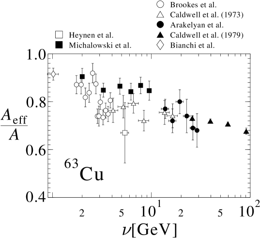
Fig. 3.3: The shadowing ratio $A_{eff}/A=\sigma_{\gamma{\mathrm{A}}}/{A\sigma_{\gamma{\mathrm{N}}}}$ for ⁶³Cu as a function of the photon energy $\nu$. The date are taken from Refs.[83, 84, 85, 86, 87, 88, 89].

Fig. 3.4: Left: NMC data [82] for the ratio $F_{2}^{{\mathrm{Sn}}}/F_{2}^{{\mathrm{C}}}$ as a function of $x$ averaged over $Q^{2}$. At large $x$ SLAC data [72] for the ratio $F_{2}^{{\mathrm{Ag}}}/F_{2}^{{\mathrm{C}}}$ are added. Right: Results for the logarithmic slope ${d}(F_{2}^{{\mathrm{Sn}}}/F_{2}^{{\mathrm{C}}})/{d}\ln Q^{2}$ from NMC [82]. The error bars represent statistical uncertainties. The band indicates the size of the systematic errors.

• Shadowing region

  Measurements of E665 [76, 77, 78] at Fermilab and NMC [71, 75, 79, 80, 81, 82] at CERN provide detailed and systematic information about the $x$- and $A$-dependence of the structure function ratios $F_{2}^{{\mathrm{A}}}/F_{2}^{{\mathrm{d}}}$. Nuclear targets ranging from He to Pb have been used. A sample of data for several nuclei is shown in Fig.3.2. While most experiments cover the region $x>10^{-4}$, the E665 collaboration provides data for $F_{2}^{{\mathrm{X}}e}/F_{2}^{{\mathrm{d}}}$ [76] down to $x\simeq 2\cdot 10^{-5}$. Given the kinematic constraints in fixed target experiments, the small $x$-region has been explored at low $Q^{2}$ only. For example, at $x\simeq 5\cdot 10^{-3}$ the typical momentum transfers are $Q^{2}\simeq 1$ GeV² [75]. At extremely small values, $x\simeq 6\cdot 10^{-5}$, one has $Q^{2}\simeq 0.03$ GeV² [76].

  In the region $5\cdot 10^{-3}<x<0.1$ the structure function ratios systematically decrease with decreasing $x$. At still smaller $x$ one enters the range of small momentum transfers, $Q^{2}\simeq 0.5$ GeV², approaching the limit of high-energy photon-nucleus interactions with real photons. As an example we show in Fig.3.3 data on shadowing for real photon scattering from ⁶³Cu.

  Shadowing systematically increases with the nuclear mass number $A$. For example, at $x\approx 0.01$ one finds $F_{2}^{{\mathrm{A}}}/F_{2}^{{\mathrm{C}}}\sim A^{\alpha-1}$ with $\alpha\approx 0.95$ [81]. A similar behavior has been observed in high-energy photonuclear cross sections [90]: their $A$-dependence is roughly $\sigma_{\gamma{\mathrm{A}}}\approx A^{0.92}\sigma_{\gamma{\mathrm{N}}}$ where $\sigma_{\gamma{\mathrm{N}}}$ is the free photon-nucleon cross section averaged over proton and neutron.

  The shadowing effect depends only weakly on the momentum transfer $Q^{2}$. The most precise investigation of this issue has been performed for the ratio of Sn and carbon structure functions presented in Fig.3.4 [82]. It reveals that shadowing decreases at most linearly with $\ln Q^{2}$ for $x<0.1$. The rate of this decrease becomes smaller with rising $x$. At $x>0.1$ no significant $Q^{2}$-dependence of $F_{2}^{{\mathrm{Sn}}}/F_{2}^{{\mathrm{C}}}$ is found.

  Shadowing has also been observed in deep-inelastic scattering from deuterium, the lightest and most weakly bound nucleus. In Fig.3.5 we show data from E665 [91] and NMC [92] for the ratio $F_{2}^{{\mathrm{d}}}/F_{2}^{{\mathrm{p}}}$ of the deuteron and proton structure functions. At $x<0.1$ this ratio is systematically smaller than one.

  
  

  Fig. 3.5: The structure function ratio $F_{2}^{{\mathrm{d}}}/F_{2}^{{\mathrm{p}}}$. Data from E665 [91] and NMC [92].

  
  

• Enhancement region

  The NMC data have established a small but statistically significant enhancement of the structure function ratio at $0.1<x<0.2$. The observed enhancement is of the order of a few percent. For carbon and calcium it amounts to typically $2\%$ [82]. The most precise measurement of this enhancement has been obtained for $F_{2}^{{\mathrm{Sn}}}/F_{2}^{{\mathrm{C}}}$ shown in Fig.3.4. Within the accuracy of the data no significant $Q^{2}$-dependence of this effect has been found in this region.

• Region of “EMC effect”

  The region of intermediate $0.2<x<0.8$ has been explored extensively at CERN and SLAC. In the range $2\,{\mathrm{GeV}}^{2}<Q^{2}<15$ GeV², data were taken by the E139 collaboration [72] for a large sample of nuclear targets between deuterium and gold. The measured structure function ratios decrease with rising $x$ and have a minimum at $x\approx 0.6$. The magnitude of this depletion grows approximately logarithmically with the nuclear mass number. The observed effect agrees well with data for the ratios of iron and nitrogen to deuterium structure functions from BCDMS taken at large $Q^{2}$ values, $14\,{\mathrm{GeV}}^{2}<Q^{2}<200$ GeV² [73, 93]. These data imply that a strong $Q^{2}$-dependence of the structure function ratios is excluded.

• Fermi motion region

  At $x>0.8$ the structure function ratios rise above unity [72], but experimental information is rather scarce. The free nucleon structure function $F_{2}^{{\mathrm{N}}}$ is known to drop as $(1-x)^{3}$ when approaching its kinematic limit at $x=1$. Clearly, even minor nuclear effects appear artificially enhanced in this kinematic range when presented in the form of the ratio $F_{2}^{{\mathrm{A}}}/F_{2}^{{\mathrm{N}}}$.

• The region $x>1$

  Data at large Bjorken $x$ and large momentum transfer, $0.7<x<1.3$ and $50\,{\mathrm{GeV}}^{2}<Q^{2}<200$ GeV², have been taken for carbon and iron by the BCDMS [94] and CCFR [95] collaborations, respectively. The results disagree with model calculations at $x\sim 1$ which account for Fermi motion effects only. For $Q^{2}<10$ GeV² data have been taken at SLAC for various nuclei [96, 97, 98, 99, 100]. Both quasielastic scattering from nucleons as well as inelastic scattering turns out to be important here.

3.4 Moments of nuclear structure functions

Given data for the ratio $F_{2}^{{\mathrm{A}}}/F_{2}^{{\mathrm{d}}}$ together with the measured deuteron structure function $F_{2}^{{\mathrm{d}}}$, the difference $F_{2}^{{\mathrm{A}}}-F_{2}^{{\mathrm{d}}}$ can be evaluated. Its integral

$$M_{2}^{{\mathrm{A}}}-M_{2}^{{\mathrm{d}}}=\intop_{0}^{1}dx_{{\mathrm{A}}}\,F_{2}^{{\mathrm{A}}}(x_{{\mathrm{A}}})-\intop_{0}^{1}dx_{{\mathrm{d}}}\,F_{2}^{{\mathrm{d}}}(x_{{\mathrm{d}}})\approx\intop_{0}^{2}dx\left(\frac{F_{2}^{{\mathrm{A}}}(x)}{F_{2}^{{\mathrm{d}}}(x)}-1+f_{M}\right)F_{2}^{{\mathrm{d}}}(x)$$ (3.11)

represents the difference of the integrated momentum fraction carried by quarks in a nucleus relative to that for deuterium. The constant $f_{M}=(AM/M_{{\mathrm{A}}}-2M/M_{{\mathrm{d}}})$ corrects for the different mass defects of bound systems. Note that in Eq.(3.11) we have omitted QCD target mass corrections [101]. An analysis based on the NMC [79] and SLAC [72] data has been performed for ${\mathrm{He}}$, ${\mathrm{C}}$ and ${\mathrm{Ca}}$ [4]. In the kinematic range covered by these experiments, $3.5\cdot 10^{-3}<x<0.8$, the difference of the structure function moments $M_{2}^{{\mathrm{A}}}-M_{2}^{{\mathrm{d}}}$ turns out to be compatible with zero. Together with the well established result of the momentum sum rule for the proton [6], one can therefore conclude that, within the accuracy of present data, quarks carry about half of the total momentum, in nuclei as well as in free nucleons.

3.5 Ratios of longitudinal and transverse cross sections

Investigations of the differences between the longitudinal-to-transverse cross section ratios $R=\sigma_{L}/\sigma_{T}$ (2.36) for different nuclei have been performed at SLAC for moderate and large values of $x$, while the region of small $x$ has been investigated by NMC. The difference $R^{{\mathrm{d}}}-R^{{\mathrm{p}}}$ is found to be compatible with zero [27, 92, 102]. Similar observations have been made for heavier targets [82, 102, 103, 104, 105]. In Fig.3.6 we show NMC data [82] for $R^{{\mathrm{Sn}}}-R^{{\mathrm{C}}}$ as a function of $x$ for an average $Q^{2}$ of about $10$ GeV². In addition we present the average values from the NMC measurement for $R^{{\mathrm{Ca}}}-R^{{\mathrm{C}}}$ [104], and for $R^{{\mathrm{Au}}}-R^{{\mathrm{Fe}}}$ from SLAC E140 [103]. All measurements are consistent with only marginal nuclear dependence of $R$. This implies that nuclear effects influence both structure functions $F_{1}$ and $F_{2}$ in a similar way, and that the ratio of nuclear cross sections directly measures the ratio of the corresponding structure functions $F_{2}$.

Fig. 3.6: NMC data [82] for $R^{{\mathrm{Sn}}}-R^{{\mathrm{C}}}$ as a function of $x$ for $\overline{Q}^{2}\approx 10$ GeV². The average values for $R^{{\mathrm{Ca}}}-R^{{\mathrm{C}}}$ [104], and $R^{{\mathrm{Au}}}-R^{{\mathrm{Fe}}}$ [103] are also shown.

3.6 Other measurements of nuclear parton distributions

Nuclear deep-inelastic scattering is sensitive only to the sum of valence and sea quark distributions (see e.g. Eq.(2.37)), weighted by their respective electric charges. In order to separate nuclear effects in the valence and sea quark sectors, and directly measure nuclear gluon distributions, other types of processes are required which we briefly summarize in the following.

3.6.1 Drell-Yan lepton pair production

In the Drell-Yan production of lepton pairs (mostly $\mu^{+}\mu^{-}$) in hadron-nucleus collisions, the underlying partonic sub-process is the annihilation of a quark and antiquark from beam and target into a time-like high energy photon, which subsequently converts into the observed dilepton. The Drell-Yan cross section reads (see e.g. [106]):

$$\frac{d^{2}\sigma}{dx_{T}dx_{B}}=\frac{4\pi\alpha^{2}}{9\,m_{l}^{2}}\,K\,\sum_{f}e_{f}^{2}\left[q_{f}^{B}(x_{B},Q^{2})\,\bar{q}_{f}^{T}(x_{T},Q^{2})+\bar{q}_{f}^{B}(x_{B},Q^{2})\,q_{f}^{T}(x_{T},Q^{2})\right],$$ (3.12)

where $m_{l}$ is the invariant mass of the produced lepton pair. The flavor dependent quark distributions of the projectile and target are denoted by $q_{f}^{B}$ and $q_{f}^{T}$, respectively. Seen from the center-of-mass frame the active quarks carry fractions $x_{B}$ and $x_{T}$ of the beam and target momenta. They are determined by the momentum component $q_{L}$ of the produced dilepton parallel to the beam, its invariant mass $m_{l}$ and the squared center-of-mass energy $s$:

$$x_{T}\,x_{B}=\frac{m_{l}^{2}}{s},\quad x_{F}=\frac{2q_{L}}{\sqrt{s}}=x_{B}-x_{T}.$$ (3.13)

Higher order QCD corrections to the production cross section (3.12) turn out to be significant. They are absorbed in the so-called “$K$-factor” and effectively double the leading order cross section.

The E772 experiment at FNAL [107] has investigated Drell-Yan dilepton production in proton-nucleus collisions at $s=1600$ GeV². At $x_{F}>0.2$ the production process is dominated by the annihilation of projectile quarks with target antiquarks. Outside the domain of quarkonium resonances, i.e. for $4\,{{\mathrm{GeV}}}<m_{l}<9$ GeV and $m_{l}>11$ GeV, this experiment explores possible modifications of nuclear sea quark distributions. In Fig.3.7 we show ratios of dimuon yields for nuclear targets and deuterium taken at $x_{F}>0$. At $x_{T}>0.1$ no significant nuclear effects have been observed within admittedly large experimental errors. This indicates the absence of strong modifications of nuclear sea quark distributions, as compared to those of free nucleons. At $x_{T}<0.1$, on the other hand, the observed attenuation for heavy nuclei implies a substantial reduction of nuclear sea quarks, in qualitative agreement with the shadowing effects observed in nuclear deep-inelastic scattering at $x<0.1$. The detailed comparison of shadowing in Drell-Yan versus DIS requires, of course, a careful separation of valence and sea quark effects as well as their $Q^{2}$ evolution [108].

Fig. 3.7: Drell-Yan dimuon yields per nucleon for ⁴⁰Ca and ¹⁸⁴W as a function of $x_{T}$ for $x_{F}>0$ [107].

3.6.2 Lepton-induced production of heavy quarks

The intrinsic heavy-quark ($c$- or $b$-quark) distributions in nucleons or nuclei are expected to be very small. Inelastic heavy-quark production is therefore assumed to receive its major contributions from photon-gluon fusion, i.e. the coupling of the exchanged virtual photon to a heavy quark pair which is attached to a gluon out of the target. This mechanism is a basic ingredient of the so-called color-singlet model [109]. In this model the cross section for heavy quark pair production is proportional to the gluon distribution of the target. A comparison of these cross sections for nucleons and nuclei can then be directly translated into a difference of the corresponding gluon distributions.

In this context NMC has analyzed $J/\psi$ production data from Sn and carbon nuclei [110]. The average ratio of the corresponding inelastic $J/\psi$ production cross sections was found slightly larger than one:

$$\frac{\sigma(\gamma^{*}+{{\mathrm{Sn}}}\rightarrow J/\psi+{{\mathrm{X}}})}{\sigma(\gamma^{*}+{{\mathrm{C}}}\rightarrow J/\psi+{{\mathrm{X}}})}=1.13\pm 0.08.$$ (3.14)

Within the color singlet model this implies an enhancement by about $10\%$ of the gluon distribution in Sn as compared to carbon in the region $x\sim 0.1$, though with large errors.

3.6.3 Neutrino scattering from nuclei

Deep-inelastic neutrino scattering permits one to separate valence and sea quark distributions. It is therefore a promising tool to investigate modifications of the different components of quark distributions in nuclei. The observed nuclear effects in neutrino experiments are qualitatively similar to the results from charged lepton scattering discussed previously [111, 112, 113, 114], although their statistical significance is poor, given the large experimental uncertainties.

4 Space-time description of deep-inelastic scattering

So far our picture of deep-inelastic scattering has been developed in momentum space. The partonic interpretation of structure functions is particularly transparent in the infinite momentum frame in which the nucleon (or nucleus) moves with (longitudinal) momentum $P\rightarrow\infty$. In this frame the Bjorken variable $x$ has a simple meaning as the fraction of the nucleon momentum carried by a parton when it is struck by the virtual photon.

For an investigation of nuclear effects in DIS the infinite momentum frame is not always optimal. Instead, it is often preferable to describe the scattering process in the laboratory frame where the target is at rest. Only in that frame the detailed knowledge about nuclear structure in terms of many-body wave functions, meson exchange currents etc. can be used efficiently. Also, the physical effects implied by characteristic nuclear scales (the nuclear radius $R_{{\mathrm{A}}}\sim A^{1/3}$ and the average nucleon-nucleon distance $d\simeq 2$ fm) are best discussed in the lab frame.

In this section we elaborate on several aspects relevant to deep-inelastic scattering as viewed in coordinate space. We first discuss the coordinate space resolution of the DIS probe. Then we introduce coordinate space distribution functions (so-called Ioffe-time distributions) of quarks and gluons and summarize results for free protons. A detailed discussion of nuclear effects in coordinate space distributions follows next. In the final part we comment on the relationship between lab frame and infinite momentum frame pictures.

4.1 Deep-inelastic scattering in coordinate space

We follow here essentially the discussion in Ref.[116] (see also [1, 117, 118, 119] and references therein). Consider the scattering from a free nucleon with momentum $P^{\mu}=(M,\mathchoice{\mbox{\boldmath$0$}}{\mbox{\boldmath$0$}}{\kern-0.20004pt\hbox{$\scriptstyle 0$}\kern-3.5pt\kern 0.39993pt\hbox{$\scriptstyle 0$}\kern-3.5pt\kern-0.20004pt\raise 0.21698pt\hbox{$\scriptstyle 0$}}{\kern-0.20004pt\hbox{$\scriptscriptstyle 0$}\kern-2.5pt\kern 0.39993pt\hbox{$\scriptscriptstyle 0$}\kern-2.5pt\kern-0.20004pt\raise 0.21698pt\hbox{$\scriptscriptstyle 0$}})$ and invariant mass $M$ in the laboratory frame. The four-momentum transfer $q^{\mu}=(\nu,\mathchoice{\mbox{\boldmath$q$}}{\mbox{\boldmath$q$}}{\kern-0.20004pt\hbox{$\scriptstyle q$}\kern-3.37604pt\kern 0.39993pt\hbox{$\scriptstyle q$}\kern-3.37604pt\kern-0.20004pt\raise 0.21698pt\hbox{$\scriptstyle q$}}{\kern-0.20004pt\hbox{$\scriptscriptstyle q$}\kern-2.41144pt\kern 0.39993pt\hbox{$\scriptscriptstyle q$}\kern-2.41144pt\kern-0.20004pt\raise 0.21698pt\hbox{$\scriptscriptstyle q$}})$, carried by the exchanged virtual photon, is taken to be in the (longitudinal) $z$-direction, $\mathchoice{\mbox{\boldmath$q$}}{\mbox{\boldmath$q$}}{\kern-0.20004pt\hbox{$\scriptstyle q$}\kern-3.37604pt\kern 0.39993pt\hbox{$\scriptstyle q$}\kern-3.37604pt\kern-0.20004pt\raise 0.21698pt\hbox{$\scriptstyle q$}}{\kern-0.20004pt\hbox{$\scriptscriptstyle q$}\kern-2.41144pt\kern 0.39993pt\hbox{$\scriptscriptstyle q$}\kern-2.41144pt\kern-0.20004pt\raise 0.21698pt\hbox{$\scriptscriptstyle q$}}=(\mathchoice{\mbox{\boldmath$0$}}{\mbox{\boldmath$0$}}{\kern-0.20004pt\hbox{$\scriptstyle 0$}\kern-3.5pt\kern 0.39993pt\hbox{$\scriptstyle 0$}\kern-3.5pt\kern-0.20004pt\raise 0.21698pt\hbox{$\scriptstyle 0$}}{\kern-0.20004pt\hbox{$\scriptscriptstyle 0$}\kern-2.5pt\kern 0.39993pt\hbox{$\scriptscriptstyle 0$}\kern-2.5pt\kern-0.20004pt\raise 0.21698pt\hbox{$\scriptscriptstyle 0$}}_{\perp},q_{3})$ with $q_{3}=\sqrt{\nu^{2}+Q^{2}}$ and $Q^{2}=-q^{2}$. In the Bjorken limit, $\nu^{2}\gg Q^{2}\gg M^{2}$ with $x=Q^{2}/(2M\nu)$ fixed, the light-cone components of the photon momentum ($q^{\pm}=\nu\pm q_{3}$) are $q^{+}\simeq 2\nu$ and $q^{-}\simeq-Mx$. All information about the response of the target to the high-energy virtual photon is in the hadronic tensor

$$W_{\mu\nu}(q,P)\sim\intop d^{4}y\,e^{iq\cdot y}\,\langle P|J_{\mu}(y)J_{\nu}(0)|P\rangle,$$ (4.1)

(see Eq.(2.24)). Using

$$q\cdot y=\frac{1}{2}\left(q^{+}y^{-}+q^{-}y^{+}\right)-\mathchoice{\mbox{\boldmath$q$}}{\mbox{\boldmath$q$}}{\kern-0.20004pt\hbox{$\scriptstyle q$}\kern-3.37604pt\kern 0.39993pt\hbox{$\scriptstyle q$}\kern-3.37604pt\kern-0.20004pt\raise 0.21698pt\hbox{$\scriptstyle q$}}{\kern-0.20004pt\hbox{$\scriptscriptstyle q$}\kern-2.41144pt\kern 0.39993pt\hbox{$\scriptscriptstyle q$}\kern-2.41144pt\kern-0.20004pt\raise 0.21698pt\hbox{$\scriptscriptstyle q$}}_{\perp}\cdot\mathchoice{\mbox{\boldmath$y$}}{\mbox{\boldmath$y$}}{\kern-0.20004pt\hbox{$\scriptstyle y$}\kern-3.6831pt\kern 0.39993pt\hbox{$\scriptstyle y$}\kern-3.6831pt\kern-0.20004pt\raise 0.21698pt\hbox{$\scriptstyle y$}}{\kern-0.20004pt\hbox{$\scriptscriptstyle y$}\kern-2.63078pt\kern 0.39993pt\hbox{$\scriptscriptstyle y$}\kern-2.63078pt\kern-0.20004pt\raise 0.21698pt\hbox{$\scriptscriptstyle y$}}_{\perp}\simeq\nu\,y^{-}-\frac{Mx}{2}\,y^{+}-\mathchoice{\mbox{\boldmath$q$}}{\mbox{\boldmath$q$}}{\kern-0.20004pt\hbox{$\scriptstyle q$}\kern-3.37604pt\kern 0.39993pt\hbox{$\scriptstyle q$}\kern-3.37604pt\kern-0.20004pt\raise 0.21698pt\hbox{$\scriptstyle q$}}{\kern-0.20004pt\hbox{$\scriptscriptstyle q$}\kern-2.41144pt\kern 0.39993pt\hbox{$\scriptscriptstyle q$}\kern-2.41144pt\kern-0.20004pt\raise 0.21698pt\hbox{$\scriptscriptstyle q$}}_{\perp}\cdot\mathchoice{\mbox{\boldmath$y$}}{\mbox{\boldmath$y$}}{\kern-0.20004pt\hbox{$\scriptstyle y$}\kern-3.6831pt\kern 0.39993pt\hbox{$\scriptstyle y$}\kern-3.6831pt\kern-0.20004pt\raise 0.21698pt\hbox{$\scriptstyle y$}}{\kern-0.20004pt\hbox{$\scriptscriptstyle y$}\kern-2.63078pt\kern 0.39993pt\hbox{$\scriptscriptstyle y$}\kern-2.63078pt\kern-0.20004pt\raise 0.21698pt\hbox{$\scriptscriptstyle y$}}_{\perp},$$ (4.2)

one obtains the following coordinate-space resolutions along the light-cone distances $y^{\pm}=t\pm y_{3}$:

$$\delta y^{-}\sim\frac{1}{\nu}\quad\mbox{and}\quad\delta y^{+}\sim\frac{1}{Mx}.$$ (4.3)

At $y^{-}=0$ the current correlation function in Eq.(4.1) is not analytic since it vanishes for $y^{+}y^{-}-{(\mathchoice{\mbox{\boldmath$y$}}{\mbox{\boldmath$y$}}{\kern-0.20004pt\hbox{$\scriptstyle y$}\kern-3.6831pt\kern 0.39993pt\hbox{$\scriptstyle y$}\kern-3.6831pt\kern-0.20004pt\raise 0.21698pt\hbox{$\scriptstyle y$}}{\kern-0.20004pt\hbox{$\scriptscriptstyle y$}\kern-2.63078pt\kern 0.39993pt\hbox{$\scriptscriptstyle y$}\kern-2.63078pt\kern-0.20004pt\raise 0.21698pt\hbox{$\scriptscriptstyle y$}}_{\perp})}^{2}<0$ because of causality (see e.g. [7]). Indeed in perturbation theory it turns out to be singular at $y^{-}=0$. Assuming that the integrand in (4.1) is an analytic function of $y^{-}$ elsewhere, this implies that $W_{\mu\nu}$ is dominated for $q^{+}\rightarrow\infty$ by contributions from $y^{-}=0$. Causality implies that, in the transverse plane, only contributions from ${(\mathchoice{\mbox{\boldmath$y$}}{\mbox{\boldmath$y$}}{\kern-0.20004pt\hbox{$\scriptstyle y$}\kern-3.6831pt\kern 0.39993pt\hbox{$\scriptstyle y$}\kern-3.6831pt\kern-0.20004pt\raise 0.21698pt\hbox{$\scriptstyle y$}}{\kern-0.20004pt\hbox{$\scriptscriptstyle y$}\kern-2.63078pt\kern 0.39993pt\hbox{$\scriptscriptstyle y$}\kern-2.63078pt\kern-0.20004pt\raise 0.21698pt\hbox{$\scriptscriptstyle y$}}_{\perp})}^{2}\simeq 1/Q^{2}$ are relevant: deep-inelastic scattering is dominated by contributions from the light cone, i.e. $y^{2}=0$.

Furthermore, Eq.(4.3) suggests that one probes increasing distances along the light cone as $x$ is decreased. Such a behavior is consistent with approximate Bjorken scaling [117]. The coordinate space analysis of nucleon structure functions in Section 4.3 confirms this conjecture. In the Bjorken limit the dominant contributions to the hadronic tensor at small $x$ come from light-like separations of order $y^{+}\sim 1/(Mx)$ between the electromagnetic currents in (4.1).

In the laboratory frame these considerations imply that deep-inelastic scattering involves a longitudinal correlation length

$$y_{3}\simeq\frac{y^{+}}{2}\equiv l$$ (4.4)

of the virtual photon. Consequently, large longitudinal distances are important in the scattering process at small $x$. This can also be deduced in the framework of time-ordered perturbation theory (see Section 4.5), where $l$ determines the typical propagation length of hadronic configurations present in the interacting photon.

The space-time pattern of deep-inelastic scattering is illustrated in Fig.4.1 in terms of the imaginary part of the forward Compton amplitude: the virtual photon interacts with partons which propagate a distance $y^{+}$ along the light cone. The characteristic laboratory frame correlation length $l$ is one half of that distance.

Fig. 4.1: Two examples of diagrams illustrating the space-time pattern of deep inelastic scattering.

4.2 Coordinate-space distribution functions

Especially when it comes to the discussion of the relevant space-time scales which govern nuclear effects in deep-inelastic scattering, it is instructive to look at quark and gluon distribution functions in coordinate rather than in momentum space. In this section we prepare the facts and return to the underlying dynamics at a later stage.

It is useful to express coordinate-space distributions in terms of a suitable dimensionless variable. For this purpose let us introduce the light-like vector $n^{\mu}$ with $n^{2}=0$ and $P\cdot n=P_{0}-P_{3}$. The hadronic tensor receives its dominant contributions from the vicinity of the light cone, where $y$ is approximately parallel to $n$. The dimensionless variable $z=y\cdot P$ then plays the role of a coordinate conjugate to Bjorken $x$. It is helpful to bear in mind that the value $z=5$ corresponds to a light-cone distance $y^{+}=2z/M\approx 2$ fm in the laboratory frame or, equivalently, to a longitudinal distance $l\equiv y^{+}/2\approx 1$ fm.

In accordance with the charge conjugation ($C$) properties of momentum-space quark and gluon distributions, one defines coordinate-space distributions by [120]:

$${\cal Q}(z,Q^{2}) \equiv \intop_{0}^{1}{d}x\,\left[q(x,Q^{2})+\bar{q}(x,Q^{2})\right]\,\sin(z\,x),$$ (4.5)

$${\cal Q}_{v}(z,Q^{2}) \equiv \intop_{0}^{1}{d}x\,\left[q(x,Q^{2})-\bar{q}(x,Q^{2})\right]\,\cos(z\,x),$$ (4.6)

$${\cal G}(z,Q^{2}) \equiv \intop_{0}^{1}{d}x\,x\,g(x,Q^{2})\,\cos(z\,x),$$ (4.7)

where $q$, $\bar{q}$ and $g$ are the momentum-space quark, antiquark and gluon distributions, respectively. Flavor indices are suppressed here for simplicity.

At leading twist accuracy, the coordinate-space distributions (4.5–4.7) are related to forward matrix elements of non-local QCD operators on the light cone [121, 122]:

$${\cal Q}(z,Q^{2}) = \frac{1}{4iP\cdot n}\,\langle P|\overline{\psi}(y)\,{n}\!\!\!/\mathchar 0\relax(y)\,\psi(0)|P\rangle_{Q^{2}}-(y\leftrightarrow-y),$$ (4.8)

$${\cal Q}_{v}(z,Q^{2}) = \frac{1}{4P\cdot n}\,\langle P|\overline{\psi}(y)\,{n}\!\!\!/\mathchar 0\relax(y)\,\psi(0)|P\rangle_{Q^{2}}+(y\leftrightarrow-y),$$ (4.9)

$${\cal G}(z,Q^{2}) = n^{\mu}n^{\nu}\frac{1}{2(P\cdot n)^{2}}\langle P|G_{\mu\lambda}(y)\,\mathchar 0\relax(y)\,G^{\lambda}_{\,\,\nu}(0)|P\rangle_{Q^{2}}.$$ (4.10)

Here $\psi$ denotes the quark field and $G_{\mu\nu}$ the gluon field strength tensor. The path-ordered exponential

$$\mathchar 0\relax(y)={{\mathrm{P}}}\exp\left[ig\,y^{\mu}\intop_{0}^{1}{d}\lambda\,A_{\mu}(\lambda y)\right]\,,$$ (4.11)

where $g$ denotes the strong coupling constant and $A^{\mu}$ the gluon field, ensures gauge invariance of the parton distributions. Note that an expansion of the right-hand side of Eqs.(4.5–4.7) and (4.8–4.10) around $y=0$ (and hence $z=y\cdot P=0$) leads to the conventional operator product expansion for parton distributions [6, 7, 8].

The functions ${\cal Q}(z)$, ${\cal Q}_{v}(z)$ and ${\cal G}(z)$ describe the mobility of partons in coordinate space. Consider, for example, the valence quark distribution ${\cal Q}_{v}(z)$. The matrix element in (4.9) has an obvious physical interpretation: as illustrated in Fig.4.1a, it measures the overlap between the nucleon ground state and a state in which one quark has been displaced along the light cone from $0$ to $y$. A different sequence is shown in Fig.4.1b. There the photon converts into a beam of partons which propagates along the light cone and interacts with partons of the target nucleon, probing primarily its sea quark and gluon content.

4.3 Coordinate-space distributions of free nucleons

In this section we discuss the properties of coordinate-space distribution functions of free nucleons. Examples of the distributions (4.8–4.10) using the CTEQ4L parametrization [123] of momentum-space quark and gluon distributions taken at a momentum scale $Q^{2}=4$ GeV², are shown in Fig. 4.2.

Fig. 4.2: Coordinate-space quark and gluon distributions resulting from the CTEQ4L parametrization of momentum-space distributions, taken at a momentum transfer $Q^{2}=4$ GeV². A sum over the $u$ and $d$ quarks is implied in the functions ${\cal Q}_{v}$ and ${\cal Q}$ [116].

Some general features can be observed: the $C$-even quark distribution ${\cal Q}(z)$ rises at small values of $z$, develops a plateau at $z\mathrel{\raise 2.58334pt\hbox{$>$}\kern-7.7778pt\lower 2.79857pt\hbox{$\sim$}}5$, and then exhibits a slow rise at very large $z$. At $z\mathrel{\raise 2.58334pt\hbox{$<$}\kern-7.7778pt\lower 2.79857pt\hbox{$\sim$}}5$, the gluon distribution function $z\,{\cal G}(z)$ behaves similarly as ${\cal Q}(z)$. For $z\mathrel{\raise 2.58334pt\hbox{$>$}\kern-7.7778pt\lower 2.79857pt\hbox{$\sim$}}5$, $z\,{\cal G}(z)$ rises somewhat faster than ${\cal Q}(z)$. The $C$-odd (or valence) quark distribution ${\cal Q}_{v}(z)$ starts with a finite value at small $z$, then begins to fall at $z\simeq 3$ and vanishes at large $z$. Recall that in the laboratory frame, the scale $z\simeq 5$ at which a significant change in the behavior of coordinate-space distributions occurs, represents a longitudinal distance comparable to the typical size of a nucleon.

Fig. 4.3: Contributions from different regions in $x$ to the ${\cal F}_{2}$ combination of coordinate-space quark and antiquark distributions at $Q^{2}=4$ GeV² [116].

At $z<5$ the coordinate-space distributions are determined by average properties of the corresponding momentum-space distribution functions as expressed by their first few moments [124, 125]. For example, the derivative of the $C$-even quark distribution ${\cal Q}(z)$ taken at $z=0$ equals the fraction of the nucleon light-cone momentum carried by quarks. The same is true for the gluon distribution $z\,{\cal G}(z)$ (the momentum fractions carried by quarks and by gluons are in fact approximately equal, a well-known experimental fact). At $z>10$ the coordinate-space distributions are determined by the small-$x$ behavior of the corresponding momentum space distributions. Assuming, for example, $q(x)\sim x^{\beta}$ for $x<0.05$ implies ${\cal Q}(z)\sim z^{-\beta-1}$ at $z>10$. Similarly, the small-$x$ behavior $g(x)\sim x^{\beta}$ leads to $z\,{\cal G}(z)\sim z^{-\beta-1}$ at large $z$. For typical values of $\beta$ as suggested by Regge phenomenology [22] one obtains ${\cal Q}_{v}\sim z^{-0.5}$ while ${\cal Q}(z)$ and $z\,{\cal G}(z)$ become constant at very large $z$.

The fact that ${\cal Q}(z)$ and $z\,{\cal G}(z)$ extend over large distances has a natural interpretation in the laboratory frame. At correlation lengths $l$ much larger than the nucleon size, both ${\cal Q}(z)$ and $z\,{\cal G}(z)$ reflect primarily the partonic structure of the photon which behaves like a high-energy beam of gluons and quark-antiquark pairs incident on the nucleon. For similar reasons, the valence quark distribution ${\cal Q}_{v}(z)$ defined in Eq.(4.9) has a pronounced tail which extends to distances beyond the nucleon radius. An antiquark in the “beam” can annihilate with a valence quark of the target nucleon, giving rise to long distance contributions in ${\cal Q}_{v}$. A detailed and instructive discussion of this frequently ignored feature can be found in Ref.[126].

Finally we illustrate the relevance of large distances in deep-inelastic scattering at small $x$. In Fig. 4.3 we show contributions to the nucleon structure function $F_{2}$ in coordinate space,

$${\cal F}_{2}(z,Q^{2})=\intop_{0}^{1}\frac{dx}{x}\,F_{2}^{{\mathrm{N}}}(x,Q^{2})\sin(z\,x),$$ (4.12)

which result from different windows of Bjorken $x$. This confirms once more that contributions from large distances $\sim 1/(Mx)$ dominate at small $x$.

4.4 Coordinate-space distributions of nuclei

The implications for scattering from nuclear targets, especially for coherence phenomena, are now obvious. If one compares, in the laboratory frame, the longitudinal correlation length $l$ from Eq.(4.4) with the average nucleon-nucleon distance in the nucleus, $d\simeq 2$ fm, one can clearly distinguish two separate regions:

1. At small distances, $l<d$, the virtual photon scatters incoherently from the individual hadronic constituents of the target nucleus. Possible modifications of the coordinate distribution functions (4.5 – 4.7) in this region are caused by bulk nuclear effects such as binding and Fermi motion.

2. At larger distances, $l>d$, it is likely that several nucleons participate collectively in the interaction. Modifications of the coordinate distribution functions are now expected to come from the coherent scattering on at least two nucleons in the target. Using $l\sim 1/(2Mx)$, this region corresponds to $x\mathrel{\raise 2.58334pt\hbox{$<$}\kern-7.7778pt\lower 2.79857pt\hbox{$\sim$}}0.05$.

This suggests that the nuclear modifications seen in coordinate-space distributions will be quite different in the regions $l>2$ fm and $l<2$ fm. This is best demonstrated by studying the ratios of nuclear and nucleon coordinate space distribution functions:

$${\cal R}_{F_{2}}(z,Q^{2}) = \frac{\intop_{0}^{A}\frac{dx}{x}\,F_{2}^{{\mathrm{A}}}(x,Q^{2})\sin(z\,x)}{\intop_{0}^{1}\frac{dx}{x}\,F_{2}^{{\mathrm{N}}}(x,Q^{2})\sin(z\,x)}=\frac{\sum_{f}e_{f}^{2}\,{\cal Q}^{{\mathrm{A}}}_{f}(z,Q^{2})}{\sum_{f}e_{f}^{2}\,{\cal Q}^{{\mathrm{N}}}_{f}(z,Q^{2})},$$ (4.13)

$${\cal R}_{v}(z,Q^{2}) = \frac{{\cal Q}^{{\mathrm{A}}}_{v}(z,Q^{2})}{{\cal Q}^{{\mathrm{N}}}_{v}(z,Q^{2})},$$ (4.14)

$${\cal R}_{\cal G}(z,Q^{2}) = \frac{z{\cal G}^{{\mathrm{A}}}(z,Q^{2})}{z{\cal G}^{{\mathrm{N}}}(z,Q^{2})}.$$ (4.15)

The ratios ${\cal R}_{F_{2}}$ have been obtained for different nuclei from an analysis of the measured momentum space structure functions [119]. Furthermore, the ratios of valence quark and gluon distributions have been calculated in [116] as sine and cosine Fourier transforms (4.5 – 4.7) of momentum space distribution functions which result from an analysis of nuclear DIS and Drell-Yan data [127] (see also Section 5.6).

Fig. 4.4: The coordinate space ratio ${\cal R}_{F_{2}}$ at $Q^{2}=5$ GeV² for ⁴He, ¹²C, and ⁴⁰Ca from Ref.[119].

In Fig.4.4 we show the ratio ${\cal R}_{F_{2}}$ for $Q^{2}=5$ GeV² taken from [119]. The most prominent feature is the pronounced depletion of ${\cal R}_{F_{2}}$ at $l>2$ fm caused by nuclear shadowing. At $l\mathrel{\raise 2.58334pt\hbox{$<$}\kern-7.7778pt\lower 2.79857pt\hbox{$\sim$}}1$ fm, nuclear modifications of ${\cal R}_{F_{2}}$ are small, and deep-inelastic scattering proceeds incoherently from the hadronic constituents of the target nucleus. The intrinsic structure of individual nucleons is evidently not much affected by nuclear mean fields. In momentum space, on the other hand, the pronounced nuclear dependence of the structure function $F_{2}^{{\mathrm{A}}}$ at $x>0.1$ evidently results from a superposition of long and short distance contributions as seen in Fig.4.3. (For a detailed discussion see Ref.[119].)

In Fig.4.5 we show the valence quark and gluon ratios ${\cal R}_{v}$ and ${\cal R}_{\cal G}$ for ⁴⁰Ca from Ref.[116]. They behave similarly as the structure function ratio ${\cal R}_{F_{2}}$, where the depletion of gluons at large distances is most pronounced. It is interesting to observe that in coordinate space, shadowing sets in at approximately the same value of $l$ for all sorts of partons. In momentum space, shadowing is found to start at different values of $x$ for different distributions [127]. Finally note that the shadowing effect continues to increase for distances larger than the nuclear diameter.

The results shown in Fig.4.5 clearly emphasize the important role of gluons in the shadowing process. Of course the incident virtual photon does not directly “see” the gluons. In the primary step the photon converts into a quark-antiquark pair. At small Bjorken-$x$, the subsequent QCD evolution of this pair rapidly induces a cascade of gluons. This cascade propagates along the light cone over distances which can exceed typical nuclear diameters by far: the high energy, high $Q^{2}$ photon behaves in part like a gluon beam which scatters coherently from the nucleus. This offers interesting new physics. The detailed QCD analysis of nuclear shadowing can in fact give information on the “cross section” $\sigma_{g{\mathrm{N}}}$ for gluons incident on nucleons, and a simple eikonal estimate using ${\cal R}_{g}$ at asymptotic distances $l$ suggests that this $\sigma_{g{\mathrm{N}}}$ is indeed large, comparable to typical hadronic cross sections (see also Refs.[128, 129]).

In summary, a coordinate space representation which selects contributions from different longitudinal distances, lucidly demonstrates that nuclear effects of the structure function $F_{2}$ and parton distributions are by far dominated by shadowing and have a surprisingly simple geometric interpretation.

Fig. 4.5: Coordinate-space ratios at $Q^{2}=4$ GeV² for gluon distributions, valence-quark distributions, and the $F_{2}$ structure function in ⁴⁰Ca [116].

4.5 Deep-inelastic scattering in standard perturbation theory

It is instructive to illustrate the previous results by looking at the lab frame space-time pattern of the (virtual) photon-nucleon interaction from the point of view of standard time-ordered perturbation theory. The two basic time orderings are shown in Figs.4.6a and 4.6b:

1. the photon hits a quark or antiquark in the target which picks up the large energy and momentum transfer;

2. the photon converts into a quark-antiquark pair which propagates and subsequently interacts with the target.

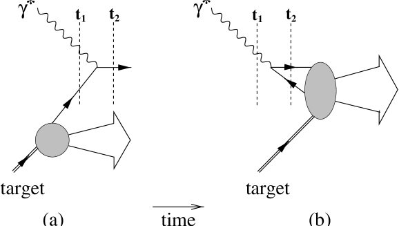
Fig. 4.6: The two possible time orderings for the interaction of a (virtual) photon with a nucleon or nuclear target: (a) the photon hits a quark in the target, (b) the photon creates a $q\bar{q}$ pair that subsequently interacts with the target.

For small Bjorken-$x$ the pair production process (b) dominates the scattering amplitude, as already mentioned. This can also be easily seen in time-ordered perturbation theory as follows (see e.g. [25] and references therein): the amplitudes ${\cal{A}}_{a}$ and ${\cal A}_{b}$ of processes (a) and (b) are roughly proportional to the inverse of their corresponding energy denominators $\mathchar 1\relax E_{a}$ and $\mathchar 1\relax E_{b}$. For large energy transfers $\nu\gg M$ one finds:

$$\mathchar 1\relax E_{a} = E_{a}(t_{2})-E_{a}(t_{1})\approx-\left<p_{q}^{2}\right>^{1/2}+\frac{\left<p_{q}^{2}\right>+Q^{2}}{2\nu},$$ (4.16)

$$\mathchar 1\relax E_{b} = E_{b}(t_{2})-E_{b}(t_{1})\approx\frac{\mu^{2}+Q^{2}}{2\nu}\;,$$ (4.17)

where $\left<p_{q}^{2}\right>^{1/2}$ is the average quark momentum in a nucleon and $\mu$ is the invariant mass of the quark-antiquark pair. We then obtain for the ratio of these amplitudes:

$$\left|\frac{{\cal A}_{a}}{{\cal A}_{b}}\right|\sim\left|\frac{\mathchar 1\relax E_{b}}{\mathchar 1\relax E_{a}}\right|\approx\frac{Mx}{\left<p_{q}^{2}\right>^{1/2}}\left(1+\frac{\mu^{2}}{Q^{2}}\right).$$ (4.18)

When analyzing the spectral representation of the scattering amplitude one observes that the bulk contribution to process (b) results from those hadronic components in the photon wave function which have a squared mass $\mu^{2}\sim Q^{2}$ (see Section 5.4.1). The ratio in Eq.(4.18) is evidently small for $x\ll 0.1$. Hence pair production, Fig.4.6b, is the leading lab frame process in the small-$x$ region. On the other hand, at $x>0.1$, both mechanisms (a) and (b) contribute.

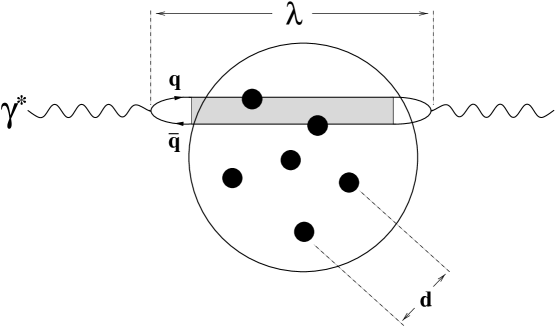
Fig. 4.7: Deep-inelastic scattering at small $x\ll 1$ in the laboratory frame proceeds via hadronic fluctuation present in the photon wave function.

In process (b) the photon couples to a quark pair which can form a complex (hadronic or quark-gluon) intermediate state and then scatters from the target. At small $x$ deep-inelastic scattering can therefore be described in the laboratory frame in terms of the interaction of quark-gluon components present in the wave function of the virtual photon (Fig.4.7). The longitudinal propagation length $\lambda$ of a specific photon-induced quark-gluon fluctuation with mass $\mu$ is given by the inverse of the energy denominator (4.17):

$$\lambda\sim\frac{1}{\mathchar 1\relax E_{b}}=\frac{2\nu}{\mu^{2}+Q^{2}}\stackrel{{\scriptstyle\mu^{2}\sim Q^{2}}}{{\relbar\joinrel\relbar\joinrel\longrightarrow}}\frac{1}{2xM},$$ (4.19)

which coincides with the longitudinal correlation length $l$ of Eq.(4.4). For $x<0.05$ the propagation length $\lambda$ exceeds the average distance between nucleons in nuclei, $\lambda>d\simeq 2\,\rm{fm}$. For a nuclear target, coherent multiple scattering of quark-gluon fluctuations of the photon from several nucleons in the nucleus can then occur, and this is clearly seen in the coordinate space analysis discussed in the previous section.

For larger values of the Bjorken variable, $x>0.2$, the propagation length of intermediate hadronic states is small, $\lambda<d$. At the same time the process in Fig.4.6a becomes prominent, i.e. the virtual photon is absorbed directly by a quark or antiquark in the target. Now the incoherent scattering from the hadronic constituents of the nucleus dominates.

4.6 Nuclear deep-inelastic scattering in the infinite momentum frame

Let us finally view the deep-inelastic scattering process in the so-called infinite momentum frame where the target momentum is large. In this frame the standard parton model applies in which a snapshot of the target at the short time scale of the interaction reveals an ensemble of almost non-interacting partons, i.e. quarks and gluons.

Consider the scattering from a nucleus which moves with large longitudinal momentum $P_{{\mathrm{A}}}\approx AP_{{\mathrm{N}}}\rightarrow\infty$, where $P_{{\mathrm{N}}}$ is the average longitudinal momentum of the bound nucleons [130, 131, 132]. The average nucleon-nucleon distance in nuclei is now Lorentz contracted as compared to the lab frame: $d^{inf}\approx d\,M_{{\mathrm{A}}}/P_{{\mathrm{A}}}\approx 2\,{\rm{fm}}\,M/P_{{\mathrm{N}}}$. On the other hand the delocalization of a parton with longitudinal momentum fraction $x$ in the nucleon is given according to the Heisenberg uncertainty principle by $\delta l\approx 1/xP_{{\mathrm{N}}}$. At small Bjorken-$x$, $x<1/d^{inf}P_{{\mathrm{N}}}\approx 0.1$, the wave functions of partons from different nucleons have a chance to overlap, i.e. $d^{inf}<\delta l$. Therefore, at $x\ll 0.1$ we expect an enhanced interaction between partons coming from different nucleons. One can anticipate that, at $x\ll 0.1$, the parton delocalization extends over the whole nucleus. This is where the quark and gluon fluctuations of the photon interact simultaneously with the parton content of several nucleons.

5 Shadowing in unpolarized deep-inelastic scattering

As outlined in Section 3.3, the most pronounced nuclear effect in lepton-nucleus DIS is shadowing. For small values of the Bjorken variable ($x<0.1$), the nuclear structure functions $F_{2}^{{\mathrm{A}}}$ are significantly reduced as compared to the free nucleon structure function $F_{2}^{{\mathrm{N}}}$. Equivalently, the virtual photon-nucleus cross section is less than $A$ times the one for free nucleons, $\sigma_{\gamma^{*}{\mathrm{A}}}<A\,\sigma_{\gamma^{*}{\mathrm{N}}}$. The analogous behavior is observed for real photons at large energies ($\nu>3\,\rm{GeV}$).

This reduction of nuclear cross sections is reminiscent of the features seen in high-energy hadron-nucleus collisions. For example, total cross sections for nucleon-nucleus scattering behave as $\sigma_{{\mathrm{NA}}}\sim A^{0.8}\,\sigma_{{\mathrm{NN}}}$ at center-of-mass energies $\sqrt{s}\sim(10$ – $25)\,{\rm GeV}^{2}$ [133]. A simple geometric picture interprets this effect as the hadron projectile interacting mainly with nucleons at the nuclear surface, leading to $\sigma_{{\mathrm{NA}}}\sim A^{2/3}$.

The quantum mechanical description of shadowing in DIS explains this phenomenon by the destructive interference of single and multiple scattering amplitudes. Multiple scattering becomes important as soon as the lab frame coherence length for the hadronic fluctuations of the photon propagator exceeds the average distance between two nucleons in the nuclear target. We have seen in our space-time discussion of Section 4 that this is precisely what happens in the region $x<0.1$ of the Bjorken variable.

The physics issue of nuclear DIS at small $x$ is therefore, roughly speaking, the optics of hadronic or quark-gluon fluctuations of the virtual photon in the nuclear medium. Diffractive phenomena play an important role in this context, as we shall demonstrate.

At extremely small $x$ (i.e. for $x<10^{-3}$) in combination with large $Q^{2}$, the measured free nucleon structure functions indicate a rapidly growing number of partons (mostly gluons). This is the domain of “high density QCD” where individual partons interact perturbatively, at large $Q^{2}$, but their number increases so strongly that effective cross sections can become large (for references see e.g. [134, 135, 136, 137, 138, 139]). It is of great interest to investigate the transition of the observed shadowing phenomena into this new domain, accessible by collider experiments, but so far unexplored for nuclear systems.

In this section we first concentrate on the relationship between diffractive photo- and leptoproduction from nucleons and shadowing in high-energy photon- and lepton-nucleus interactions. Then we investigate perturbative and non-perturbative QCD aspects of shadowing. After that we summarize existing models which successfully describe data. Finally we outline implications of shadowing for nuclear parton distributions.

5.1 Diffractive production and nuclear shadowing

In the shadowing region, diffractive photo- and leptoproduction of high energy hadrons gives a substantial contribution to the (virtual) photon-nucleon cross section as discussed in Section 2.6.4. This suggests that the diffractive excitation of hadronic states, $\gamma^{*}{{\mathrm{N}}}\rightarrow{{\mathrm{XN}}}$, and their coherent interaction with several nucleons inside the target plays an important role for shadowing in high energy photon-nucleus scattering, in a similar way as for hadron-nucleus collisions. For this effect to be significant, the following two conditions have to be met in the laboratory frame:

1. The longitudinal propagation length, or coherence length,

   $$\lambda=\frac{2\nu}{M_{{\mathrm{X}}}^{2}+Q^{2}}$$ (5.1)

   of the diffractively produced hadronic state of invariant mass $M_{{\mathrm{X}}}$, Eq.(4.19), must exceed the average nucleon-nucleon distance in nuclei:

   $$\lambda>d\simeq 2\,\mbox{fm}.$$ (5.2)

2. In addition, the mean free path $l_{{\mathrm{X}}}=\left(\rho\,\sigma_{{\mathrm{XN}}}\right)^{-1}$ of the diffractively produced system in the nuclear medium must be sufficiently short, at least smaller than the nuclear radius

Note that the mean free path of photons in a nucleus with density $\rho$ amounts to $l_{\gamma}\approx(\rho\,\sigma_{\gamma{\mathrm{N}}})^{-1}\approx 550\,{\rm fm}$, which is much larger than any nuclear scale. Consequently “bare” photons do not scatter coherently from several nucleons and therefore do not contribute to shadowing.

Shadowing results from the coherent scattering of a hadronic fluctuation from at least two nucleons in the target, i.e. for $\lambda>d$. Since the longitudinal propagation length $\lambda$ of a diffractively produced hadronic state ${{\mathrm{X}}}$ decreases with its mass $M_{{\mathrm{X}}}$, low mass excitations with $M_{{\mathrm{X}}}\mathrel{\raise 2.58334pt\hbox{$<$}\kern-7.7778pt\lower 2.79857pt\hbox{$\sim$}}1\,{\rm GeV}$ are relevant for the onset of shadowing. Equation (5.2) tells again that shadowing in deep-inelastic scattering at $Q^{2}\gg 1\,\rm{GeV^{2}}$ should start at $x\approx 0.1$, in accordance with the observed effect and in close correspondence with the space-time picture described in Section 4.

For real photons diffractive processes at low mass are dominated by the excitation of the $\rho$- and $\omega$-meson. Significant contributions to double scattering and hence to shadowing are therefore expected if the photon energy $\nu$ exceeds about $3$ GeV, in line with the experimental data.

Consider now the scattering process in the laboratory frame. Realistic nuclear wave functions are well established only in this frame (with the exception of recent efforts to construct relativistic nuclear model wave functions on the light front, see e.g. [140 – 146]). Later, in Section 5.5, we comment on nuclear shadowing as seen in the Breit frame. We first neglect effects due to nuclear binding, Fermi-motion and non-nucleonic degrees of freedom in nuclei. They are relevant at moderate and large values of the Bjorken variable, $x>0.1$, as discussed in Section 6.

The (virtual) photon-nucleus cross section can be separated into a piece which accounts for the incoherent scattering from individual nucleons, and a correction from the coherent interaction with several nucleons:

$$\sigma_{\gamma^{*}{{\mathrm{A}}}}=Z\,\sigma_{\gamma^{*}{{\mathrm{p}}}}+(A-Z)\,\sigma_{\gamma^{*}{{\mathrm{n}}}}+\delta\sigma_{\gamma^{*}{{\mathrm{A}}}}.$$ (5.3)

The single scattering part is the incoherent sum of photon-nucleon cross sections, where $Z$ is the nuclear charge. The multiple scattering correction can be expanded in contributions which account for the scattering from $n\geq 2$ nucleons. Expressed in terms of the corresponding multiple scattering amplitudes ${\cal A}^{(n)}_{\gamma^{*}{\mathrm{A}}}$ we have:

$$\delta\sigma_{\gamma^{*}{{\mathrm{A}}}}=\frac{1}{2M_{{\mathrm{A}}}\nu}\sum_{n=2}^{A}{{\mathrm{Im}}}\,{\cal A}_{\gamma^{*}{{\mathrm{A}}}}^{(n)},$$ (5.4)

where the photon flux (2.32) is taken in the limit $x\ll 1$. The leading contribution to nuclear shadowing comes from double scattering. Its mechanism is best illustrated for a deuterium target on which we focus next.

5.1.1 Shadowing in deuterium

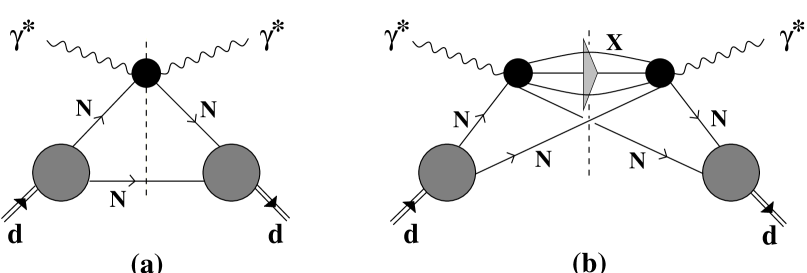
Fig. 5.1: Single (a) and double (b) scattering contribution to virtual photon-deuteron scattering. The corresponding cross sections are obtained from the imaginary part of the forward scattering amplitude indicated by the dashed line.

In this section we review the basic mechanism of shadowing in real and virtual photon-deuteron scattering at high energies $\nu$, or equivalently, small $x$. The $\gamma^{*}$-deuteron cross section can be written as the sum of single and double scattering parts as illustrated in Fig.5.1:

$$\sigma_{\gamma^{*}{\mathrm{d}}}=\sigma_{\gamma^{*}{{\mathrm{p}}}}+\sigma_{\gamma^{*}{{\mathrm{n}}}}+\delta\sigma_{\gamma^{*}{{\mathrm{d}}}}.$$ (5.5)

The first two terms describe the incoherent scattering of the (virtual) photon from the proton or neutron, while

$$\delta\sigma_{\gamma^{*}{{\mathrm{d}}}}=\frac{1}{2M_{{\mathrm{d}}}\nu}\,{{\mathrm{Im}}}\,{\cal A}^{(2)}_{\gamma^{*}{{\mathrm{d}}}}$$ (5.6)

accounts for the coherent interaction of the projectile with both nucleons.

For large energies, $\nu>3$ GeV, or small values of the Bjorken variable, $x<0.1$, the double scattering amplitude ${\cal A}^{(2)}_{\gamma^{*}{{\mathrm{d}}}}$ is dominated by the diffractive excitation of hadronic intermediate states (Fig.5.1 b) described by the amplitude $T_{\gamma^{*}{{\mathrm{N\rightarrow XN}}}}$. At the high energies involved it is a good approximation to neglect the real part of this amplitude. In fact, we expect ${\rm{Re}}\,T_{\gamma^{*}{\mathrm{N\rightarrow XN}}}\mathrel{\raise 2.58334pt\hbox{$<$}\kern-7.7778pt\lower 2.79857pt\hbox{$\sim$}}0.15\,{\rm{Im}}\,T_{\gamma^{*}{\mathrm{N\rightarrow XN}}}$ by analogy with high-energy hadron-hadron scattering amplitudes (see e.g. [21]). When including such non-zero real parts, the double scattering contribution changes by less than $10\%$ [147]. We neglect the spin and isospin dependence for unpolarized scattering [70]. Of course, these degrees of freedom play a crucial role in polarized scattering as we will discuss in Section 7.3.

Treating the deuteron target in the non-relativistic limit gives [148, 149, 150, 151]:

$${\cal A}_{\gamma^{*}{{\mathrm{d}}}}^{(2)} = -\frac{2}{M}\intop d^{3}r\,|\psi_{{\mathrm{d}}}(\mathchoice{\mbox{\boldmath$r$}}{\mbox{\boldmath$r$}}{\kern-0.20004pt\hbox{$\scriptstyle r$}\kern-3.35255pt\kern 0.39993pt\hbox{$\scriptstyle r$}\kern-3.35255pt\kern-0.20004pt\raise 0.21698pt\hbox{$\scriptstyle r$}}{\kern-0.20004pt\hbox{$\scriptscriptstyle r$}\kern-2.39467pt\kern 0.39993pt\hbox{$\scriptscriptstyle r$}\kern-2.39467pt\kern-0.20004pt\raise 0.21698pt\hbox{$\scriptscriptstyle r$}})|^{2}$$ (5.7)

$$\times\sum_{{\mathrm{X}}}\intop\frac{d^{3}k}{(2\pi)^{3}}\,T_{\gamma^{*}{{\mathrm{N\rightarrow XN}}}}(k)\,\frac{e^{i\mathchoice{\mbox{\boldmath$k$}}{\mbox{\boldmath$k$}}{\kern-0.14003pt\hbox{$\scriptstyle k$}\kern-2.7052pt\kern 0.27995pt\hbox{$\scriptstyle k$}\kern-2.7052pt\kern-0.14003pt\raise 0.15189pt\hbox{$\scriptstyle k$}}{\kern-0.14003pt\hbox{$\scriptscriptstyle k$}\kern-1.93228pt\kern 0.27995pt\hbox{$\scriptscriptstyle k$}\kern-1.93228pt\kern-0.14003pt\raise 0.15189pt\hbox{$\scriptscriptstyle k$}}\cdot\mathchoice{\mbox{\boldmath$r$}}{\mbox{\boldmath$r$}}{\kern-0.14003pt\hbox{$\scriptstyle r$}\kern-2.34679pt\kern 0.27995pt\hbox{$\scriptstyle r$}\kern-2.34679pt\kern-0.14003pt\raise 0.15189pt\hbox{$\scriptstyle r$}}{\kern-0.14003pt\hbox{$\scriptscriptstyle r$}\kern-1.67627pt\kern 0.27995pt\hbox{$\scriptscriptstyle r$}\kern-1.67627pt\kern-0.14003pt\raise 0.15189pt\hbox{$\scriptscriptstyle r$}}}}{(q_{0}-k_{0})^{2}-\mathchoice{\mbox{\boldmath$k$}}{\mbox{\boldmath$k$}}{\kern-0.20004pt\hbox{$\scriptstyle k$}\kern-3.86458pt\kern 0.39993pt\hbox{$\scriptstyle k$}\kern-3.86458pt\kern-0.20004pt\raise 0.21698pt\hbox{$\scriptstyle k$}}{\kern-0.20004pt\hbox{$\scriptscriptstyle k$}\kern-2.7604pt\kern 0.39993pt\hbox{$\scriptscriptstyle k$}\kern-2.7604pt\kern-0.20004pt\raise 0.21698pt\hbox{$\scriptscriptstyle k$}}_{\perp}^{2}-(q_{3}-k_{3})^{2}-M_{{\mathrm{X}}}^{2}+i\epsilon}\,T_{{{\mathrm{XN}}}\rightarrow\gamma^{*}{{\mathrm{N}}}}(k),$$

where $k^{\mu}=(k_{0},\mathchoice{\mbox{\boldmath$k$}}{\mbox{\boldmath$k$}}{\kern-0.20004pt\hbox{$\scriptstyle k$}\kern-3.86458pt\kern 0.39993pt\hbox{$\scriptstyle k$}\kern-3.86458pt\kern-0.20004pt\raise 0.21698pt\hbox{$\scriptstyle k$}}{\kern-0.20004pt\hbox{$\scriptscriptstyle k$}\kern-2.7604pt\kern 0.39993pt\hbox{$\scriptscriptstyle k$}\kern-2.7604pt\kern-0.20004pt\raise 0.21698pt\hbox{$\scriptscriptstyle k$}})$ with $\mathchoice{\mbox{\boldmath$k$}}{\mbox{\boldmath$k$}}{\kern-0.20004pt\hbox{$\scriptstyle k$}\kern-3.86458pt\kern 0.39993pt\hbox{$\scriptstyle k$}\kern-3.86458pt\kern-0.20004pt\raise 0.21698pt\hbox{$\scriptstyle k$}}{\kern-0.20004pt\hbox{$\scriptscriptstyle k$}\kern-2.7604pt\kern 0.39993pt\hbox{$\scriptscriptstyle k$}\kern-2.7604pt\kern-0.20004pt\raise 0.21698pt\hbox{$\scriptscriptstyle k$}}=(\mathchoice{\mbox{\boldmath$k$}}{\mbox{\boldmath$k$}}{\kern-0.20004pt\hbox{$\scriptstyle k$}\kern-3.86458pt\kern 0.39993pt\hbox{$\scriptstyle k$}\kern-3.86458pt\kern-0.20004pt\raise 0.21698pt\hbox{$\scriptstyle k$}}{\kern-0.20004pt\hbox{$\scriptscriptstyle k$}\kern-2.7604pt\kern 0.39993pt\hbox{$\scriptscriptstyle k$}\kern-2.7604pt\kern-0.20004pt\raise 0.21698pt\hbox{$\scriptscriptstyle k$}}_{\perp},k_{3})$ is the four-momentum transfered to the nucleon, and $\psi_{{\mathrm{d}}}$ is the deuteron wave function normalized as $\intop d^{3}r\,|\psi_{{\mathrm{d}}}(\mathchoice{\mbox{\boldmath$r$}}{\mbox{\boldmath$r$}}{\kern-0.20004pt\hbox{$\scriptstyle r$}\kern-3.35255pt\kern 0.39993pt\hbox{$\scriptstyle r$}\kern-3.35255pt\kern-0.20004pt\raise 0.21698pt\hbox{$\scriptstyle r$}}{\kern-0.20004pt\hbox{$\scriptscriptstyle r$}\kern-2.39467pt\kern 0.39993pt\hbox{$\scriptscriptstyle r$}\kern-2.39467pt\kern-0.20004pt\raise 0.21698pt\hbox{$\scriptscriptstyle r$}})|^{2}=1$. The sum is taken over all diffractively excited hadronic states with invariant mass $M_{{\mathrm{X}}}$ and four-momentum $p_{{\mathrm{X}}}=q-k$. We write

$$\sum_{{\mathrm{X}}}{|T_{\gamma^{*}{{\mathrm{N\rightarrow XN}}}}|^{2}}=64\,\pi\,M^{2}\nu^{2}\intop_{4m_{\pi}^{2}}^{W^{2}}dM_{{\mathrm{X}}}^{2}\,\frac{d^{2}\sigma^{diff}_{\gamma^{*}{{\mathrm{N}}}}}{dM_{{\mathrm{X}}}^{2}dt}$$ (5.8)

in terms of the diffractive production cross section, with $t=k^{2}$. The limits of integration define the kinematically permitted range of diffractive excitations, with their invariant mass $M_{{\mathrm{X}}}$ above the two-pion production threshold and limited by the center-of-mass energy $W=\sqrt{s}$ of the scattering process. We introduce the spin-averaged deuteron form factor,

$$S_{{\mathrm{d}}}(\mathchoice{\mbox{\boldmath$k$}}{\mbox{\boldmath$k$}}{\kern-0.20004pt\hbox{$\scriptstyle k$}\kern-3.86458pt\kern 0.39993pt\hbox{$\scriptstyle k$}\kern-3.86458pt\kern-0.20004pt\raise 0.21698pt\hbox{$\scriptstyle k$}}{\kern-0.20004pt\hbox{$\scriptscriptstyle k$}\kern-2.7604pt\kern 0.39993pt\hbox{$\scriptscriptstyle k$}\kern-2.7604pt\kern-0.20004pt\raise 0.21698pt\hbox{$\scriptscriptstyle k$}})=\intop d^{3}r\,e^{i\mathchoice{\mbox{\boldmath$k$}}{\mbox{\boldmath$k$}}{\kern-0.14003pt\hbox{$\scriptstyle k$}\kern-2.7052pt\kern 0.27995pt\hbox{$\scriptstyle k$}\kern-2.7052pt\kern-0.14003pt\raise 0.15189pt\hbox{$\scriptstyle k$}}{\kern-0.14003pt\hbox{$\scriptscriptstyle k$}\kern-1.93228pt\kern 0.27995pt\hbox{$\scriptscriptstyle k$}\kern-1.93228pt\kern-0.14003pt\raise 0.15189pt\hbox{$\scriptscriptstyle k$}}\cdot\mathchoice{\mbox{\boldmath$r$}}{\mbox{\boldmath$r$}}{\kern-0.14003pt\hbox{$\scriptstyle r$}\kern-2.34679pt\kern 0.27995pt\hbox{$\scriptstyle r$}\kern-2.34679pt\kern-0.14003pt\raise 0.15189pt\hbox{$\scriptstyle r$}}{\kern-0.14003pt\hbox{$\scriptscriptstyle r$}\kern-1.67627pt\kern 0.27995pt\hbox{$\scriptscriptstyle r$}\kern-1.67627pt\kern-0.14003pt\raise 0.15189pt\hbox{$\scriptscriptstyle r$}}}\,|\psi_{{\mathrm{d}}}(\mathchoice{\mbox{\boldmath$r$}}{\mbox{\boldmath$r$}}{\kern-0.20004pt\hbox{$\scriptstyle r$}\kern-3.35255pt\kern 0.39993pt\hbox{$\scriptstyle r$}\kern-3.35255pt\kern-0.20004pt\raise 0.21698pt\hbox{$\scriptstyle r$}}{\kern-0.20004pt\hbox{$\scriptscriptstyle r$}\kern-2.39467pt\kern 0.39993pt\hbox{$\scriptscriptstyle r$}\kern-2.39467pt\kern-0.20004pt\raise 0.21698pt\hbox{$\scriptscriptstyle r$}})|^{2},$$ (5.9)

perform the integration over the longitudinal momentum transfer in Eq.(5.7) and then take the imaginary part of the amplitude ${\cal A}_{\gamma^{*}{{\mathrm{d}}}}^{(2)}$. Actually $k_{3}$ is simply fixed by energy-momentum conservation:

$$k_{3}\approx\frac{Q^{2}+M_{{\mathrm{X}}}^{2}}{2\nu}=\frac{1}{\lambda},$$ (5.10)

which coincides with the inverse of the longitudinal propagation length (4.19) of the intermediate hadronic state. Note that the minimal momentum transfer required to produce a hadronic state diffractively from a nucleon at rest amounts to $t_{min}\approx-k_{3}^{2}(M_{{\mathrm{X}}})$.

When all steps are carried out, the result for the double scattering correction is [148, 149]

$$\delta\sigma_{\gamma^{*}{{\mathrm{d}}}}=-\frac{2}{\pi}\intop d^{2}k_{\perp}\intop_{4m_{\pi}^{2}}^{W^{2}}dM_{{\mathrm{X}}}^{2}\,\,S_{{\mathrm{d}}}(\mathchoice{\mbox{\boldmath$k$}}{\mbox{\boldmath$k$}}{\kern-0.20004pt\hbox{$\scriptstyle k$}\kern-3.86458pt\kern 0.39993pt\hbox{$\scriptstyle k$}\kern-3.86458pt\kern-0.20004pt\raise 0.21698pt\hbox{$\scriptstyle k$}}{\kern-0.20004pt\hbox{$\scriptscriptstyle k$}\kern-2.7604pt\kern 0.39993pt\hbox{$\scriptscriptstyle k$}\kern-2.7604pt\kern-0.20004pt\raise 0.21698pt\hbox{$\scriptscriptstyle k$}}_{\perp},k_{3}\approx\lambda^{-1}(M_{{\mathrm{X}}}))\,\,\frac{d^{2}\sigma^{diff}_{\gamma^{*}{{\mathrm{N}}}}}{dM_{{\mathrm{X}}}^{2}dt}\,.$$ (5.11)

This equation establishes the close relationship between shadowing in deep-inelastic scattering and diffractive hadron production. It becomes even more transparent for $x\ll 0.1$, i.e. large $\lambda$. In this limit the magnitude of shadowing is determined just by the ratio of diffractive and total $\gamma^{*}{\mathrm{N}}$ cross sections. To verify this let us parametrize the $t$-dependence of the diffractive production cross section entering in Eq.(5.11) as

$$\frac{d^{2}\sigma^{diff}_{\gamma^{*}{{\mathrm{N}}}}}{dM_{{\mathrm{X}}}^{2}dt}=e^{-{B}|t|}\,\left.\frac{d^{2}\sigma^{diff}_{\gamma^{*}{{\mathrm{N}}}}}{dM_{{\mathrm{X}}}^{2}dt}\right|_{t=0}\approx e^{-{B}\mathchoice{\mbox{\boldmath$k$}}{\mbox{\boldmath$k$}}{\kern-0.14003pt\hbox{$\scriptstyle k$}\kern-2.7052pt\kern 0.27995pt\hbox{$\scriptstyle k$}\kern-2.7052pt\kern-0.14003pt\raise 0.15189pt\hbox{$\scriptstyle k$}}{\kern-0.14003pt\hbox{$\scriptscriptstyle k$}\kern-1.93228pt\kern 0.27995pt\hbox{$\scriptscriptstyle k$}\kern-1.93228pt\kern-0.14003pt\raise 0.15189pt\hbox{$\scriptscriptstyle k$}}_{\perp}^{2}}\,\left.\frac{d^{2}\sigma^{diff}_{\gamma^{*}{{\mathrm{N}}}}}{dM_{{\mathrm{X}}}^{2}dt}\right|_{t=0},$$ (5.12)

neglecting the $k_{3}$ dependence of $t$. Data from FNAL and HERA on diffractive photo- and leptoproduction of hadrons with mass $M_{{\mathrm{X}}}^{2}>3$ GeV² give $B\simeq(5\dots 7)\,$GeV^-2 [53, 58, 59]. In the diffractive production of low mass vector mesons ($\rho,\omega$ and $\phi$) from nucleons, a range of values $B\simeq(4\dots 10)\,$GeV^-2 has been found, depending on $Q^{2}$ and on the incident photon energy (for a review and references see e.g. [49, 64]). Clearly, the soft deuteron form factor selects momenta such that the double scattering correction in (5.11) is dominated by diffractive production in the direction of the incident photon.

In Fig.5.2 we show the deuteron form factor (5.9) weighted by the exponential $t$-dependence (5.12) and integrated over transverse momentum,

$${\cal F}_{{\mathrm{d}}}^{B}(\lambda^{-1})\equiv{\intop}\frac{d^{2}k_{\perp}}{(2\pi)^{2}}\,S_{{\mathrm{d}}}(\mathchoice{\mbox{\boldmath$k$}}{\mbox{\boldmath$k$}}{\kern-0.20004pt\hbox{$\scriptstyle k$}\kern-3.86458pt\kern 0.39993pt\hbox{$\scriptstyle k$}\kern-3.86458pt\kern-0.20004pt\raise 0.21698pt\hbox{$\scriptstyle k$}}{\kern-0.20004pt\hbox{$\scriptscriptstyle k$}\kern-2.7604pt\kern 0.39993pt\hbox{$\scriptscriptstyle k$}\kern-2.7604pt\kern-0.20004pt\raise 0.21698pt\hbox{$\scriptscriptstyle k$}}_{\perp},k_{3}=\lambda^{-1})\,e^{-B\mathchoice{\mbox{\boldmath$k$}}{\mbox{\boldmath$k$}}{\kern-0.14003pt\hbox{$\scriptstyle k$}\kern-2.7052pt\kern 0.27995pt\hbox{$\scriptstyle k$}\kern-2.7052pt\kern-0.14003pt\raise 0.15189pt\hbox{$\scriptstyle k$}}{\kern-0.14003pt\hbox{$\scriptscriptstyle k$}\kern-1.93228pt\kern 0.27995pt\hbox{$\scriptscriptstyle k$}\kern-1.93228pt\kern-0.14003pt\raise 0.15189pt\hbox{$\scriptscriptstyle k$}}_{\perp}^{2}},$$ (5.13)

as obtained with the Paris nucleon-nucleon potential [152] for a slope parameter $B=8$ GeV^-2. We observe ${\cal F}_{{\mathrm{d}}}^{B}\approx constant$ as long as the longitudinal propagation length $\lambda$ exceeds the deuteron size $\langle r^{2}\rangle_{{\mathrm{d}}}^{1/2}\approx 4\,fm$. From Eq.(5.2) one then finds that hadronic states with an invariant mass

$$M_{{\mathrm{X}}}^{2}<M_{max}^{2}=\frac{W^{2}+Q^{2}}{M\langle r^{2}\rangle^{1/2}_{{\mathrm{d}}}}-Q^{2}$$ (5.14)

contribute dominantly to double scattering. Combining Eqs.(5.11) and (5.14) gives the following approximate expression for the shadowing correction in the limit of large longitudinal propagation length $\lambda$:

$$\delta\sigma_{\gamma^{*}{{\mathrm{d}}}} \approx -8\pi\,{\cal F}_{{\mathrm{d}}}^{B}(\lambda^{-1}\rightarrow 0)\,\left.\intop_{4m_{\pi}^{2}}^{M_{max}^{2}}dM_{{\mathrm{X}}}^{2}\,\frac{d\sigma^{diff}_{\gamma^{*}{{\mathrm{N}}}}}{dM_{{\mathrm{X}}}^{2}dt}\right|_{t=0}\approx-8\pi{\cal F}_{{\mathrm{d}}}^{B}(0)\,B\,\sigma^{diff}_{\gamma^{*}{{\mathrm{N}}}}.$$ (5.15)

In the last step we have neglected contributions to the integrated diffractive production cross section $\sigma^{diff}_{\gamma^{*}{{\mathrm{N}}}}$ from hadronic states with invariant masses $M_{max}<M_{{\mathrm{X}}}<W$. Since $d\sigma^{diff}_{\gamma^{*}{{\mathrm{N}}}}/dM_{{\mathrm{X}}}^{2}$ drops strongly for large $M_{{\mathrm{X}}}$ as discussed in Section 2.6.4, this approximation is justified at large center of mass energies $W$ or, equivalently, at small $x$. For the ratio between deuteron and free nucleon structure functions we then obtain:

$$R_{{\mathrm{d}}}=\frac{F_{2}^{{\mathrm{d}}}}{F_{2}^{{\mathrm{N}}}}=\frac{\sigma_{\gamma^{*}{\mathrm{d}}}}{2\,\sigma_{\gamma^{*}{\mathrm{N}}}}\approx 1-4\pi\,{\cal F}_{{\mathrm{d}}}^{B}(0)\,B\,\frac{\sigma^{diff}_{\gamma^{*}{{\mathrm{N}}}}}{\sigma_{\gamma^{*}{{\mathrm{N}}}}}.$$ (5.16)

We use ${\sigma^{diff}_{\gamma^{*}{{\mathrm{N}}}}}/{\sigma_{\gamma^{*}{{\mathrm{N}}}}}\approx 0.1$ for the fraction of diffractive events in deep-inelastic scattering from free nucleons, as suggested by experiment (see Section 2.6.4). Furthermore we take $B=8$ GeV^-2. One finds that shadowing at $x\ll 0.1$ in deuterium amounts to about $2\%$, i.e. $R_{{\mathrm{d}}}\approx 0.98$. The effect is small because of the large average proton-neutron distance in the deuteron, but the result agrees well with the experimental data shown in Fig.3.5.

Fig. 5.2: Integrated deuteron form factor ${\cal F}_{{\mathrm{d}}}^{B}$ from Eq.(5.13) for an average slope $B=8$ GeV². The dotted curve corresponds to $B=0$.

5.1.2 Shadowing for heavy nuclei

The diffractive production of hadrons from single nucleons also controls shadowing in heavier nuclei for which this effect is far more pronounced than in the deuteron. It is an empirical fact that nuclear shadowing increases with the nuclear mass number $A$ of the target (see Section 3.3). For $A>2$ the hadronic state which is produced in the interaction of the photon with one of the nucleons in the target may scatter coherently from more than two nucleons. However, double scattering still dominates since the probability that the propagating hadron interacts with several nucleons along its path decreases with the number of scatterers. The double scattering contribution to the total photon-nucleus cross section $\sigma_{\gamma^{*}{{\mathrm{A}}}}$ is obtained by straightforward generalization of the deuteron result (5.11) [149, 150]:

$$\sigma_{\gamma^{*}{{\mathrm{A}}}}^{(2)} = -8\pi\intop d{{}^{2}b}\intop_{-\infty}^{+\infty}dz_{1}\intop_{z_{1}}^{+\infty}dz_{2}\,\rho_{{\mathrm{A}}}^{(2)}(\mathchoice{\mbox{\boldmath$b$}}{\mbox{\boldmath$b$}}{\kern-0.20004pt\hbox{$\scriptstyle b$}\kern-3.00417pt\kern 0.39993pt\hbox{$\scriptstyle b$}\kern-3.00417pt\kern-0.20004pt\raise 0.21698pt\hbox{$\scriptstyle b$}}{\kern-0.20004pt\hbox{$\scriptscriptstyle b$}\kern-2.14583pt\kern 0.39993pt\hbox{$\scriptscriptstyle b$}\kern-2.14583pt\kern-0.20004pt\raise 0.21698pt\hbox{$\scriptscriptstyle b$}},z_{1};\mathchoice{\mbox{\boldmath$b$}}{\mbox{\boldmath$b$}}{\kern-0.20004pt\hbox{$\scriptstyle b$}\kern-3.00417pt\kern 0.39993pt\hbox{$\scriptstyle b$}\kern-3.00417pt\kern-0.20004pt\raise 0.21698pt\hbox{$\scriptstyle b$}}{\kern-0.20004pt\hbox{$\scriptscriptstyle b$}\kern-2.14583pt\kern 0.39993pt\hbox{$\scriptscriptstyle b$}\kern-2.14583pt\kern-0.20004pt\raise 0.21698pt\hbox{$\scriptscriptstyle b$}},z_{2})\,\cdot$$ (5.17)

$$\hskip 85.35826pt\intop_{4m_{\pi}^{2}}^{W^{2}}dM_{{\mathrm{X}}}^{2}\cos\left[(z_{2}-z_{1})/\lambda\right]\left.\frac{d^{2}\sigma^{diff}_{\gamma^{*}{{\mathrm{N}}}}}{dM_{{\mathrm{X}}}^{2}dt}\right|_{t\approx 0}.$$

As illustrated in Fig.5.3 a diffractive state with invariant mass $M_{{\mathrm{X}}}$ is produced in the interaction of the photon with a nucleon located at position $(\mathchoice{\mbox{\boldmath$b$}}{\mbox{\boldmath$b$}}{\kern-0.20004pt\hbox{$\scriptstyle b$}\kern-3.00417pt\kern 0.39993pt\hbox{$\scriptstyle b$}\kern-3.00417pt\kern-0.20004pt\raise 0.21698pt\hbox{$\scriptstyle b$}}{\kern-0.20004pt\hbox{$\scriptscriptstyle b$}\kern-2.14583pt\kern 0.39993pt\hbox{$\scriptscriptstyle b$}\kern-2.14583pt\kern-0.20004pt\raise 0.21698pt\hbox{$\scriptscriptstyle b$}},z_{1})$ in the target. The hadronic excitation propagates at fixed impact parameter $b$ and then interacts with a second nucleon at $z_{2}$. The probability to find two nucleons in the target at the same impact parameter is described by the two-body density $\rho_{{\mathrm{A}}}^{(2)}(\mathchoice{\mbox{\boldmath$b$}}{\mbox{\boldmath$b$}}{\kern-0.20004pt\hbox{$\scriptstyle b$}\kern-3.00417pt\kern 0.39993pt\hbox{$\scriptstyle b$}\kern-3.00417pt\kern-0.20004pt\raise 0.21698pt\hbox{$\scriptstyle b$}}{\kern-0.20004pt\hbox{$\scriptscriptstyle b$}\kern-2.14583pt\kern 0.39993pt\hbox{$\scriptscriptstyle b$}\kern-2.14583pt\kern-0.20004pt\raise 0.21698pt\hbox{$\scriptscriptstyle b$}},z_{1};\mathchoice{\mbox{\boldmath$b$}}{\mbox{\boldmath$b$}}{\kern-0.20004pt\hbox{$\scriptstyle b$}\kern-3.00417pt\kern 0.39993pt\hbox{$\scriptstyle b$}\kern-3.00417pt\kern-0.20004pt\raise 0.21698pt\hbox{$\scriptstyle b$}}{\kern-0.20004pt\hbox{$\scriptscriptstyle b$}\kern-2.14583pt\kern 0.39993pt\hbox{$\scriptscriptstyle b$}\kern-2.14583pt\kern-0.20004pt\raise 0.21698pt\hbox{$\scriptscriptstyle b$}},z_{2})$ normalized as $\intop d^{3}r\,d^{3}r^{\prime}\,\rho_{{\mathrm{A}}}^{(2)}(\mathchoice{\mbox{\boldmath$r$}}{\mbox{\boldmath$r$}}{\kern-0.20004pt\hbox{$\scriptstyle r$}\kern-3.35255pt\kern 0.39993pt\hbox{$\scriptstyle r$}\kern-3.35255pt\kern-0.20004pt\raise 0.21698pt\hbox{$\scriptstyle r$}}{\kern-0.20004pt\hbox{$\scriptscriptstyle r$}\kern-2.39467pt\kern 0.39993pt\hbox{$\scriptscriptstyle r$}\kern-2.39467pt\kern-0.20004pt\raise 0.21698pt\hbox{$\scriptscriptstyle r$}},\mathchoice{\mbox{\boldmath$r$}}{\mbox{\boldmath$r$}}{\kern-0.20004pt\hbox{$\scriptstyle r$}\kern-3.35255pt\kern 0.39993pt\hbox{$\scriptstyle r$}\kern-3.35255pt\kern-0.20004pt\raise 0.21698pt\hbox{$\scriptstyle r$}}{\kern-0.20004pt\hbox{$\scriptscriptstyle r$}\kern-2.39467pt\kern 0.39993pt\hbox{$\scriptscriptstyle r$}\kern-2.39467pt\kern-0.20004pt\raise 0.21698pt\hbox{$\scriptscriptstyle r$}}\,^{\prime})=A^{2}$. The $\cos[(z_{2}-z_{1})/\lambda]$ factor in Eq.(5.17) implies that only diffractively excited hadrons with a longitudinal propagation length larger than the average nucleon-nucleon distance in the target, $\lambda>d\simeq 2\,\rm{fm}$, can contribute significantly to double scattering.

Note that nuclear short-range correlations are relevant only if the coherence length of the diffractively excited states is comparable to the range of the short-range repulsive part of the nucleon-nucleon force, i.e. for $\lambda\mathrel{\raise 2.58334pt\hbox{$<$}\kern-7.7778pt\lower 2.79857pt\hbox{$\sim$}}0.5\,\rm{fm}$. In this case the shadowing effect is negligible. Nuclear correlations are therefore not important in the shadowing domain and the target can be considered as an ensemble of independent nucleons with $\rho_{{\mathrm{A}}}^{(2)}(\mathchoice{\mbox{\boldmath$r$}}{\mbox{\boldmath$r$}}{\kern-0.20004pt\hbox{$\scriptstyle r$}\kern-3.35255pt\kern 0.39993pt\hbox{$\scriptstyle r$}\kern-3.35255pt\kern-0.20004pt\raise 0.21698pt\hbox{$\scriptstyle r$}}{\kern-0.20004pt\hbox{$\scriptscriptstyle r$}\kern-2.39467pt\kern 0.39993pt\hbox{$\scriptscriptstyle r$}\kern-2.39467pt\kern-0.20004pt\raise 0.21698pt\hbox{$\scriptscriptstyle r$}},\mathchoice{\mbox{\boldmath$r$}}{\mbox{\boldmath$r$}}{\kern-0.20004pt\hbox{$\scriptstyle r$}\kern-3.35255pt\kern 0.39993pt\hbox{$\scriptstyle r$}\kern-3.35255pt\kern-0.20004pt\raise 0.21698pt\hbox{$\scriptstyle r$}}{\kern-0.20004pt\hbox{$\scriptscriptstyle r$}\kern-2.39467pt\kern 0.39993pt\hbox{$\scriptscriptstyle r$}\kern-2.39467pt\kern-0.20004pt\raise 0.21698pt\hbox{$\scriptscriptstyle r$}}\,^{\prime})\approx\rho_{{\mathrm{A}}}(\mathchoice{\mbox{\boldmath$r$}}{\mbox{\boldmath$r$}}{\kern-0.20004pt\hbox{$\scriptstyle r$}\kern-3.35255pt\kern 0.39993pt\hbox{$\scriptstyle r$}\kern-3.35255pt\kern-0.20004pt\raise 0.21698pt\hbox{$\scriptstyle r$}}{\kern-0.20004pt\hbox{$\scriptscriptstyle r$}\kern-2.39467pt\kern 0.39993pt\hbox{$\scriptscriptstyle r$}\kern-2.39467pt\kern-0.20004pt\raise 0.21698pt\hbox{$\scriptscriptstyle r$}})\rho_{{\mathrm{A}}}(\mathchoice{\mbox{\boldmath$r$}}{\mbox{\boldmath$r$}}{\kern-0.20004pt\hbox{$\scriptstyle r$}\kern-3.35255pt\kern 0.39993pt\hbox{$\scriptstyle r$}\kern-3.35255pt\kern-0.20004pt\raise 0.21698pt\hbox{$\scriptstyle r$}}{\kern-0.20004pt\hbox{$\scriptscriptstyle r$}\kern-2.39467pt\kern 0.39993pt\hbox{$\scriptscriptstyle r$}\kern-2.39467pt\kern-0.20004pt\raise 0.21698pt\hbox{$\scriptscriptstyle r$}}\,^{\prime})$, where $\rho_{{\mathrm{A}}}$ is the nuclear one-body density [153, 154].

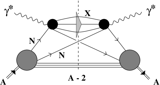
Fig. 5.3: Double scattering contribution to deep-inelastic scattering from nuclei.

With increasing photon energies or decreasing $x$ down to $x\ll 0.1$, the longitudinal propagation length of diffractively excited hadrons rises and eventually reaches nuclear dimensions. Then interactions of the excited hadronic states with several nucleons in the target become important. A simple way to account for those is a frequently used equation derived by Karmanov and Kondratyuk [155]:

$$\delta\sigma_{\gamma^{*}{{\mathrm{A}}}} = -8\pi\intop d{{}^{2}b}\intop_{-\infty}^{+\infty}dz_{1}\intop_{z_{1}}^{+\infty}dz_{2}\,\rho_{{\mathrm{A}}}(\mathchoice{\mbox{\boldmath$b$}}{\mbox{\boldmath$b$}}{\kern-0.20004pt\hbox{$\scriptstyle b$}\kern-3.00417pt\kern 0.39993pt\hbox{$\scriptstyle b$}\kern-3.00417pt\kern-0.20004pt\raise 0.21698pt\hbox{$\scriptstyle b$}}{\kern-0.20004pt\hbox{$\scriptscriptstyle b$}\kern-2.14583pt\kern 0.39993pt\hbox{$\scriptscriptstyle b$}\kern-2.14583pt\kern-0.20004pt\raise 0.21698pt\hbox{$\scriptscriptstyle b$}},z_{1})\,\rho_{{\mathrm{A}}}(\mathchoice{\mbox{\boldmath$b$}}{\mbox{\boldmath$b$}}{\kern-0.20004pt\hbox{$\scriptstyle b$}\kern-3.00417pt\kern 0.39993pt\hbox{$\scriptstyle b$}\kern-3.00417pt\kern-0.20004pt\raise 0.21698pt\hbox{$\scriptstyle b$}}{\kern-0.20004pt\hbox{$\scriptscriptstyle b$}\kern-2.14583pt\kern 0.39993pt\hbox{$\scriptscriptstyle b$}\kern-2.14583pt\kern-0.20004pt\raise 0.21698pt\hbox{$\scriptscriptstyle b$}},z_{2})\cdot$$ (5.18)

$$\hskip 5.69046pt\intop_{4m_{\pi}^{2}}^{W^{2}}dM_{{\mathrm{X}}}^{2}\cos\left[(z_{2}-z_{1})/\lambda\right]\left.\frac{d^{2}\sigma^{diff}_{\gamma^{*}{{\mathrm{N}}}}}{dM_{{\mathrm{X}}}^{2}dt}\right|_{t\approx 0}\exp\left[-\frac{\sigma_{{{\mathrm{XN}}}}}{2}\intop_{z_{1}}^{z_{2}}dz\,\rho_{{\mathrm{A}}}(\mathchoice{\mbox{\boldmath$b$}}{\mbox{\boldmath$b$}}{\kern-0.20004pt\hbox{$\scriptstyle b$}\kern-3.00417pt\kern 0.39993pt\hbox{$\scriptstyle b$}\kern-3.00417pt\kern-0.20004pt\raise 0.21698pt\hbox{$\scriptstyle b$}}{\kern-0.20004pt\hbox{$\scriptscriptstyle b$}\kern-2.14583pt\kern 0.39993pt\hbox{$\scriptscriptstyle b$}\kern-2.14583pt\kern-0.20004pt\raise 0.21698pt\hbox{$\scriptscriptstyle b$}},z)\right].$$

The exponential attenuation factor describes the elastic re-scattering of the diffractively produced hadronic states from the remaining nucleons in the target. The hadron-nucleon scattering amplitudes are assumed to be purely imaginary and enter in Eq.(5.18) through the cross sections $\sigma_{{{\mathrm{XN}}}}$.

Equation (5.18) has been applied in several investigations of nuclear shadowing using different models for the diffractive photoproduction cross section. The more detailed results are discussed in Section 5.4, but we can get a simple estimate of nuclear shadowing at small Bjorken-$x$ already by just looking at the relative amount of diffraction in DIS from free nucleons [66]. We restrict ourselves to the double scattering correction (5.17). For $x\ll 0.1$, the coherence length $\lambda$ of the hadronic states which dominate diffractive production in Eq.(5.17), exceed the diameter of the target nucleus. In the limit $\lambda\rightarrow\infty$ we find:

$$\sigma^{(2)}_{\gamma^{*}{{\mathrm{A}}}}\simeq-8\pi\,B\,\sigma^{diff}_{\gamma^{*}{{\mathrm{N}}}}\intop d{{}^{2}b}\intop_{-\infty}^{+\infty}dz_{1}\intop_{z_{1}}^{+\infty}dz_{2}\,\rho_{{\mathrm{A}}}(\mathchoice{\mbox{\boldmath$b$}}{\mbox{\boldmath$b$}}{\kern-0.20004pt\hbox{$\scriptstyle b$}\kern-3.00417pt\kern 0.39993pt\hbox{$\scriptstyle b$}\kern-3.00417pt\kern-0.20004pt\raise 0.21698pt\hbox{$\scriptstyle b$}}{\kern-0.20004pt\hbox{$\scriptscriptstyle b$}\kern-2.14583pt\kern 0.39993pt\hbox{$\scriptscriptstyle b$}\kern-2.14583pt\kern-0.20004pt\raise 0.21698pt\hbox{$\scriptscriptstyle b$}},z_{1})\,\rho_{{\mathrm{A}}}(\mathchoice{\mbox{\boldmath$b$}}{\mbox{\boldmath$b$}}{\kern-0.20004pt\hbox{$\scriptstyle b$}\kern-3.00417pt\kern 0.39993pt\hbox{$\scriptstyle b$}\kern-3.00417pt\kern-0.20004pt\raise 0.21698pt\hbox{$\scriptstyle b$}}{\kern-0.20004pt\hbox{$\scriptscriptstyle b$}\kern-2.14583pt\kern 0.39993pt\hbox{$\scriptscriptstyle b$}\kern-2.14583pt\kern-0.20004pt\raise 0.21698pt\hbox{$\scriptscriptstyle b$}},z_{2}).$$ (5.19)

The slope parameter $B$ and the integrated diffractive production cross section $\sigma^{diff}_{\gamma^{*}{{\mathrm{N}}}}$ have been introduced as in Eqs.(5.12, 5.15).

For the nuclear densities in Eq.(5.19) we use Gaussian,

$$\rho_{{\mathrm{A}}}(\mathchoice{\mbox{\boldmath$r$}}{\mbox{\boldmath$r$}}{\kern-0.20004pt\hbox{$\scriptstyle r$}\kern-3.35255pt\kern 0.39993pt\hbox{$\scriptstyle r$}\kern-3.35255pt\kern-0.20004pt\raise 0.21698pt\hbox{$\scriptstyle r$}}{\kern-0.20004pt\hbox{$\scriptscriptstyle r$}\kern-2.39467pt\kern 0.39993pt\hbox{$\scriptscriptstyle r$}\kern-2.39467pt\kern-0.20004pt\raise 0.21698pt\hbox{$\scriptscriptstyle r$}})=A\,\left(\frac{3}{2\,\pi\,\langle r^{2}\rangle_{{\mathrm{A}}}}\right)^{3/2}\,\exp\left(-\frac{3\,\mathchoice{\mbox{\boldmath$r$}}{\mbox{\boldmath$r$}}{\kern-0.20004pt\hbox{$\scriptstyle r$}\kern-3.35255pt\kern 0.39993pt\hbox{$\scriptstyle r$}\kern-3.35255pt\kern-0.20004pt\raise 0.21698pt\hbox{$\scriptstyle r$}}{\kern-0.20004pt\hbox{$\scriptscriptstyle r$}\kern-2.39467pt\kern 0.39993pt\hbox{$\scriptscriptstyle r$}\kern-2.39467pt\kern-0.20004pt\raise 0.21698pt\hbox{$\scriptscriptstyle r$}}\,^{2}}{2\,\langle r^{2}\rangle_{{\mathrm{A}}}}\right),$$ (5.20)

and square-well parametrizations,

$$\rho_{{\mathrm{A}}}(\mathchoice{\mbox{\boldmath$r$}}{\mbox{\boldmath$r$}}{\kern-0.20004pt\hbox{$\scriptstyle r$}\kern-3.35255pt\kern 0.39993pt\hbox{$\scriptstyle r$}\kern-3.35255pt\kern-0.20004pt\raise 0.21698pt\hbox{$\scriptstyle r$}}{\kern-0.20004pt\hbox{$\scriptscriptstyle r$}\kern-2.39467pt\kern 0.39993pt\hbox{$\scriptscriptstyle r$}\kern-2.39467pt\kern-0.20004pt\raise 0.21698pt\hbox{$\scriptscriptstyle r$}})=\left\{\begin{array}[]{l}A\frac{3}{4\pi}\left(\frac{3}{5\,\langle r^{2}\rangle_{{\mathrm{A}}}}\right)^{3/2}\quad\mbox{for}\quad r<\sqrt{\frac{5}{3}}\,\langle r^{2}\rangle_{{\mathrm{A}}}^{1/2},\\ 0\hskip 85.35826pt\mbox{otherwise},\end{array}\right.$$

with the mean square radius $\langle r^{2}\rangle_{{\mathrm{A}}}=\intop d^{3}r\,r^{2}\,\rho_{{\mathrm{A}}}(r)/A$. For both cases the shadowing ratio $R_{{\mathrm{A}}}=\sigma_{\gamma^{*}{{\mathrm{A}}}}/{A\sigma_{\gamma^{*}{{\mathrm{N}}}}}$ is easily worked out:

$$R_{{\mathrm{A}}}\simeq 1-{\cal C}\,A\,\left(\frac{B}{\langle r^{2}\rangle_{{\mathrm{A}}}}\right)\frac{\sigma^{diff}_{\gamma^{*}{{\mathrm{N}}}}}{\sigma_{\gamma^{*}{{\mathrm{N}}}}}.$$ (5.21)

For Gaussian nuclear densities one finds ${\cal C}=3$, while ${\cal C}=2.7$ in the square-well case.

Using again typical values for the ratio of diffractive and total $\gamma^{*}{\mathrm{N}}$ cross sections, ${\sigma^{diff}_{\gamma^{*}{{\mathrm{N}}}}}/{\sigma_{\gamma^{*}{{\mathrm{N}}}}}\simeq 0.1$, and for the slope parameter, $B\simeq 8$ GeV^-2, the magnitude of $R_{{\mathrm{A}}}$ comes out in very reasonable agreement with experimental values as shown in Table 1.

	6Li	12C	40Ca	131Xe
$R_{{\mathrm{A}}}$	$0.93$	$0.84$	$0.73$	$0.65$
$R_{{\mathrm{A}}}^{exp.}$	$0.94\pm 0.07$	$0.87\pm 0.10$	$0.77\pm 0.07$	$0.67\pm 0.09$

Table 1: The shadowing ratio $R_{{\mathrm{A}}}$ estimated according to Eq.(5.21) in comparison to experimental data for various nuclei. The data are taken from Ref.[75, 76, 77] at the smallest kinematically accessible values of Bjorken-$x$ (namely, $x\simeq 10^{-4}$).

This estimate may be simple (in fact, higher order multiple scattering must be included in a more detailed analysis) but it certainly confirms that shadowing in nuclear DIS is governed by the coherent interaction of diffractively produced states with several nucleons in the target nucleus. A more detailed investigation of the connection between HERA data on diffraction and shadowing effects measured at CERN and FNAL can be found in Ref.[156].

Inelastic transitions between different hadronic states are neglected in Eq.(5.18). They cannot be treated in a model-independent way. Estimates of such higher order diffractive dissociation contributions have been performed for high-energy hadron-nucleus scattering [133, 157]. In the case of neutron-nucleus collisions at center-of-mass energies $s\sim 200\,\rm{GeV^{2}}$ they amount to about $5\%$ of the total reaction cross section. For rising energies the relative importance of inelastic transitions is expected to grow [157].

Fig. 5.4: The quantity $\log\left(1-R_{{\mathrm{A}}}\right)$ as a function of $\log x$ for data taken on lead [77]. The dashed line corresponds to the asymtotic energy dependence (5.23) with $\varepsilon=0.1$.

Given the important role of diffractive production, we can now enter into a more detailed discussion of the $x$-dependence of shadowing. The coherence lengths $\lambda$ of hadronic states with small masses become comparable with nuclear dimensions for $x<0.1$. As $\lambda$ increases with decreasing $x$, the shadowing effect grows steadily for $x\mathrel{\raise 2.58334pt\hbox{$<$}\kern-7.7778pt\lower 2.79857pt\hbox{$\sim$}}0.05$. At $x\ll 0.1$ it is also the energy dependence of the diffractive production cross section and of the hadron-nucleon cross section $\sigma_{{\mathrm{XN}}}$ which influences the $x$-dependence of shadowing.

Consider the shadowing ratio $R_{{\mathrm{A}}}={\sigma_{\gamma^{*}{{\mathrm{A}}}}}/{A\sigma_{\gamma^{*}{{\mathrm{N}}}}}=1-\delta\sigma_{\gamma^{*}{\mathrm{A}}}/{A\sigma_{\gamma^{*}{{\mathrm{N}}}}}$, parametrized as:

$$R_{{\mathrm{A}}}-1=-c\,\left(\frac{1}{x}\right)^{\varepsilon},$$ (5.22)

with a constant $c$ at small $Q^{2}$ where data are actually taken, and a characteristic exponent $\epsilon$. At asymptotically large energies Regge phenomenology suggests $\varepsilon\simeq 0.1$ (see Section 2.6.4) .

In Fig.5.4 we show the quantity

$$\log\left(1-R_{{\mathrm{A}}}\right)=\log c-\varepsilon\,\log x,$$ (5.23)

plotted versus $\log x$ in comparison with data taken on Pb at small $Q^{2}$. This plot confirms that, for $x<3\cdot 10^{-3}$, the shadowing effect indeed approaches the high-energy behavior expected from the Regge limit of diffractive production. Deviations from this asymptotic behavior at larger values of $x$ indicate how shadowing gradually builds up as the coherence length $\lambda\propto x^{-1}$ starts to exceed nuclear length scales for low mass diffractively produced states. At sufficiently high energy or small $x$, the coherence length becomes comparable to nuclear dimensions even for heavy hadronic intermediate states. Once a major fraction of diffractively produced states contribute to shadowing it starts to approach its asymtotic high-energy behavior. Note this asymptotic behavior sets in when the coherence lengths $\lambda_{\rm X}$ of low mass hadronic fluctuations of the photon exceed by far the dimension of the nucleus. For example at $x=3\cdot 10^{-3}$ and $Q^{2}\simeq 0.7$ GeV², which corresponds to the onset of the asymptotic behavior in Fig.5.4, the $\rho$ meson coherence length becomes $\lambda_{\rho}\simeq 36$ fm.

5.1.3 Shadowing for real photons

Data on the diffractive production of hadrons in high-energy photon-nucleon interactions have been summarized in Section 2.8. They are useful to gain insight into the relative importance of $\rho$, $\omega$ and $\phi$ mesons, as compared to heavier states, for nuclear shadowing with real photons.

Diffractive $\gamma{{\mathrm{N}}}\rightarrow{{\mathrm{XN}}}$ production with $M_{{\mathrm{X}}}\mathrel{\raise 2.58334pt\hbox{$<$}\kern-7.7778pt\lower 2.79857pt\hbox{$\sim$}}1$ GeV involves primarily the light vector mesons $\rho$, $\omega$ and $\phi$. Nuclear shadowing at photon energies $\nu$ up to about $200$ GeV is largely determined by the coherent multiple scattering of those diffractively produced vector mesons. Their propagation lengths $\lambda\simeq 2\nu/m_{{\mathrm{V}}}^{2}$ easily exceed nuclear dimensions as soon as $\nu>20$ GeV. With rising energies additional contributions to shadowing from diffractively produced states with larger masses, $M_{{\mathrm{X}}}>1$ GeV, become increasingly important.

This behavior is illustrated for DIS from deuterium in Fig.5.5, where we show the ratio of the total photon-deuteron cross section compared to the free photon-nucleon cross section, $R_{{\mathrm{d}}}=\sigma_{\gamma{{\mathrm{d}}}}/2\sigma_{\gamma{{\mathrm{N}}}}$, from Ref.[147]. The empirical photon-proton cross section from [158] has been used for $\sigma_{\gamma{{\mathrm{N}}}}$. The shadowing correction (5.11) has been calculated using a fit for the diffractive photon-nucleon cross section from Ref.[147].

The observed energy dependence of shadowing in Fig.5.5 results from two sources as pointed out previously: the dependence of the diffractive and total photon-nucleon cross sections on energy implies $R_{{\mathrm{d}}}-1\sim\nu^{0.1}$ for the shadowing ratio. An additional increase of shadowing with rising energy $\nu$ comes from diffractively produced states with large mass, $M_{{\mathrm{X}}}>1$ GeV, which become relevant at high energies.

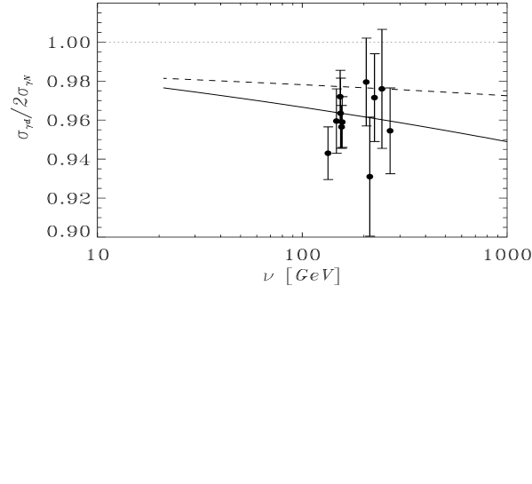
Fig. 5.5: The shadowing ratio $R_{{\mathrm{d}}}=\sigma_{\gamma{\mathrm{d}}}/2\sigma_{\gamma{\mathrm{N}}}$ as a function of the photon energy. The dashed line shows the vector meson contribution. The experimental data are taken from the E665 collaboration [91]. (The energy values of the data have to be understood as average values which correspond to different $x$-bins.)

5.1.4 Shadowing in DIS at small and moderate $Q^{2}$

So far nuclear shadowing has been measured only in fixed target experiments. The kinematic conditions of such experiments imply that the data for $x<0.01$ had to be taken at small four-momentum transfers, $\overline{Q^{2}}\mathrel{\raise 2.58334pt\hbox{$<$}\kern-7.7778pt\lower 2.79857pt\hbox{$\sim$}}1$ GeV², as discussed in Section 3.3.1. The corresponding energy transfers are typically $50\,{\rm GeV}<\nu<300\,{\rm GeV}$. The conclusions just drawn for real photons apply here too: nuclear shadowing as measured by E665 and NMC receives major contributions from the diffractive production and multiple scattering of vector mesons.

In the intermediate range $0.01<x<0.1$, on the other hand, the E665 and NMC measurements involve momentum transfers up to $Q^{2}\sim 30\,{{\mathrm{GeV}}}^{2}$. At $Q^{2}>1$ GeV² vector meson contributions to diffraction and shadowing decrease (Section 2.6.4) and hadronic states with masses $M_{{\mathrm{X}}}^{2}\sim Q^{2}$ become relevant. The data reveal that the $Q^{2}$-dependence of nuclear shadowing is very weak (Section 3.3.1). This suggests that high-mass hadronic components of the photon which dominate the measured nuclear shadowing at $Q^{2}>1$ GeV², interact strongly with the target, just like ordinary hadrons. The following section gives a schematic view of the scales involved, as outlined in Ref.[159].

5.2 Sizes, scales and shadowing

Consider DIS at small $x$ in the lab frame. In this frame of reference the important feature is the nuclear interaction of hadronic fluctuations of the virtual photon (see Section 4). Since the photon and its hadronic configurations carry high energy, the transverse separations and longitudinal momenta of their quark and gluon constituents are approximately conserved during the scattering process. These hadronic configurations can be classified as “small” or “large”, depending on their transverse extension. “Large” configurations have hadronic sizes of order $\mathchar 3\relax_{{\mathrm{QCD}}}^{-1}\sim 1$ fm, whereas “small” configurations are characterized by sizes which scale as $Q^{-1}$.

The contribution of a given hadronic fluctuation, ${\mathrm{h}}$, to the photon-nucleon interaction cross section is determined by its probability weight $w_{\gamma^{*}{\mathrm{h}}}$ in the photon wave function, multiplied by its cross section $\sigma_{{\mathrm{hN}}}$. The virtual photon-nucleon cross section is:

$$\sigma_{\gamma^{*}{\mathrm{N}}}=\sum_{{\mathrm{h}}}w_{\gamma^{*}{\mathrm{h}}}\,\sigma_{{\mathrm{hN}}}.$$ (5.24)

The coherent interaction of the virtual photon with several nucleons behaves differently. For example, the contribution of a hadronic fluctuation to double scattering, which dominates shadowing, is proportional to its weight in the photon wave function multiplied by the square of its interaction cross section. The double scattering correction to virtual photon-nucleus scattering is:

$$\sigma_{\gamma^{*}{\mathrm{A}}}^{(2)}\sim\sum_{{\mathrm{h}}}w_{\gamma^{*}{\mathrm{h}}}\,(\sigma_{{\mathrm{hN}}})^{2}.$$ (5.25)

Now, the probability to find a quark-gluon configuration of large size is suppressed (up to possible logarithmic terms) by $\mathchar 3\relax_{{{\mathrm{QCD}}}}^{2}/Q^{2}$ as compared to configurations with small transverse sizes. On the other hand the interaction cross sections of hadronic fluctuations are proportional to their squared transverse radii. These properties and their consequences for the cross sections in Eqs.(5.24) and (5.25) are summarized in Table 2.

fluctuation h	$w_{\gamma^{*}{\mathrm{h}}}$	$\sigma_{{\mathrm{hN}}}$	$w_{\gamma^{*}{\mathrm{h}}}\,\sigma_{{\mathrm{hN}}}$	$w_{\gamma^{*}{\mathrm{h}}}\,(\sigma_{{\mathrm{hN}}})^{2}$
small size	$1$	$1/Q^{2}$	$1/Q^{2}$	$1/Q^{4}$
large size	$\mathchar 3\relax_{{{\mathrm{QCD}}}}^{2}/Q^{2}$	$1/\mathchar 3\relax_{{{\mathrm{QCD}}}}^{2}$	$1/Q^{2}$	$1/(\mathchar 3\relax_{{{\mathrm{QCD}}}}^{2}Q^{2})$

Table 2: Relative contributions of small- and large-size hadronic components of a virtual photon to DIS and shadowing at large $Q^{2}$ [159].

For the scattering from individual nucleons one finds that both, large- and small-size configurations give leading contributions $\sim 1/Q^{2}$ to the photon-nucleon cross section (5.24). On the other hand contributions from small-size components to the shadowing correction $\sigma_{\gamma^{*}{\mathrm{A}}}^{(2)}$ are suppressed by an additional power $1/Q^{2}$ as compared to large-size configurations (apart from contributions related to diffractive production from the whole nucleus, not considered in this schematic picture).

In view of these scale considerations, we can now understand some of the previously mentioned empirical facts which, on first sight, seemed unrelated:

• Nuclear shadowing varies only weakly with $Q^{2}$.

• The energy dependence of nuclear shadowing for $x\mathrel{\raise 2.58334pt\hbox{$<$}\kern-7.7778pt\lower 2.79857pt\hbox{$\sim$}}0.01$, as measured with fixed target experiments at CERN and FNAL, is reminiscent of hadron-nucleus collisions.

These features follow from the fact that, to leading order in $Q^{2}$, shadowing is primarily determined by the interaction of large-size hadronic fluctuations of the exchanged photon, even at large $Q^{2}$. These hadronic configurations are expected to interact like ordinary hadrons.

Note, those observations can be applied to diffraction as well as to shadowing, given that the two phenomena are closely connected as established in the previous sections: diffraction is also a scaling effect, i.e. it survives at large $Q^{2}$. Its energy dependence is expected to behave similarly as in hadron collisions. (For limitations to this simple picture see Sections 5.3 and 8.2.)

5.3 Nuclear shadowing and parton configurations of the photon

The results of the previous sections are eludicated by making contact with the underlying basic QCD and the parton structure of the virtual photon. The photon wave function can be decomposed in a Fock space expansion,

$$|\gamma\rangle=c_{0}|\gamma_{0}\rangle+c_{q\bar{q}}|q\bar{q}\rangle+c_{q\bar{q}g}|q\bar{q}g\rangle+\dots,$$ (5.26)

in terms of a “bare” photon state $|\gamma_{0}\rangle$ and partonic (quark-antiquark and gluonic) components. At large $Q^{2}$ the minimal Fock component $|q\bar{q}\rangle$ dominates the hadronic part of $|\gamma\rangle$, higher Fock states enter with powers of the strong coupling $\alpha_{s}$. Let us now have a closer look at this minimal Fock component.

Consider a virtual photon of four-momentum $q^{\mu}=(\nu,\mathchoice{\mbox{\boldmath$q$}}{\mbox{\boldmath$q$}}{\kern-0.20004pt\hbox{$\scriptstyle q$}\kern-3.37604pt\kern 0.39993pt\hbox{$\scriptstyle q$}\kern-3.37604pt\kern-0.20004pt\raise 0.21698pt\hbox{$\scriptstyle q$}}{\kern-0.20004pt\hbox{$\scriptscriptstyle q$}\kern-2.41144pt\kern 0.39993pt\hbox{$\scriptscriptstyle q$}\kern-2.41144pt\kern-0.20004pt\raise 0.21698pt\hbox{$\scriptscriptstyle q$}})$, with $\mathchoice{\mbox{\boldmath$q$}}{\mbox{\boldmath$q$}}{\kern-0.20004pt\hbox{$\scriptstyle q$}\kern-3.37604pt\kern 0.39993pt\hbox{$\scriptstyle q$}\kern-3.37604pt\kern-0.20004pt\raise 0.21698pt\hbox{$\scriptstyle q$}}{\kern-0.20004pt\hbox{$\scriptscriptstyle q$}\kern-2.41144pt\kern 0.39993pt\hbox{$\scriptscriptstyle q$}\kern-2.41144pt\kern-0.20004pt\raise 0.21698pt\hbox{$\scriptscriptstyle q$}}=(0,0,q_{3})$ and $q_{3}>0$ defining the longitudinal direction, and $Q^{2}=-q^{2}$. Let this photon split into a quark-antiquark pair as sketched in Fig.5.6. The quark has a four-momentum $k^{\mu}=(k_{0},\mathchoice{\mbox{\boldmath$k$}}{\mbox{\boldmath$k$}}{\kern-0.20004pt\hbox{$\scriptstyle k$}\kern-3.86458pt\kern 0.39993pt\hbox{$\scriptstyle k$}\kern-3.86458pt\kern-0.20004pt\raise 0.21698pt\hbox{$\scriptstyle k$}}{\kern-0.20004pt\hbox{$\scriptscriptstyle k$}\kern-2.7604pt\kern 0.39993pt\hbox{$\scriptscriptstyle k$}\kern-2.7604pt\kern-0.20004pt\raise 0.21698pt\hbox{$\scriptscriptstyle k$}})$ with $\mathchoice{\mbox{\boldmath$k$}}{\mbox{\boldmath$k$}}{\kern-0.20004pt\hbox{$\scriptstyle k$}\kern-3.86458pt\kern 0.39993pt\hbox{$\scriptstyle k$}\kern-3.86458pt\kern-0.20004pt\raise 0.21698pt\hbox{$\scriptstyle k$}}{\kern-0.20004pt\hbox{$\scriptscriptstyle k$}\kern-2.7604pt\kern 0.39993pt\hbox{$\scriptscriptstyle k$}\kern-2.7604pt\kern-0.20004pt\raise 0.21698pt\hbox{$\scriptscriptstyle k$}}=(\mathchoice{\mbox{\boldmath$k$}}{\mbox{\boldmath$k$}}{\kern-0.20004pt\hbox{$\scriptstyle k$}\kern-3.86458pt\kern 0.39993pt\hbox{$\scriptstyle k$}\kern-3.86458pt\kern-0.20004pt\raise 0.21698pt\hbox{$\scriptstyle k$}}{\kern-0.20004pt\hbox{$\scriptscriptstyle k$}\kern-2.7604pt\kern 0.39993pt\hbox{$\scriptscriptstyle k$}\kern-2.7604pt\kern-0.20004pt\raise 0.21698pt\hbox{$\scriptscriptstyle k$}}_{\perp},k_{3})$. The fraction of the photon light-cone momentum carried by the quark is

$$\xi=\frac{k^{+}}{q^{+}}=\frac{k_{0}+k_{3}}{\nu+q_{3}}.$$ (5.27)

The momentum fraction of the antiquark with $\bar{k}^{\mu}=q^{\mu}-k^{\mu}$ is obviously $1-\xi$.

For the longitudinally polarized photon, the wave function of its minimal $q\bar{q}$ fluctuation in momentum space is proportional to the longitudinal component of the quark pair current, multiplied by its propagator $\left[Q^{2}+\frac{m_{q}^{2}+k_{\perp}^{2}}{\xi(1-\xi)}\right]^{-1}$ where $m_{q}$ is the quark mass [160]. The quantity

$$M_{{\mathrm{X}}}^{2}=\frac{m_{q}^{2}+k_{\perp}^{2}}{\xi(1-\xi)}$$ (5.28)

can be interpreted as the squared effective mass of the propagating $q\bar{q}$ pair.

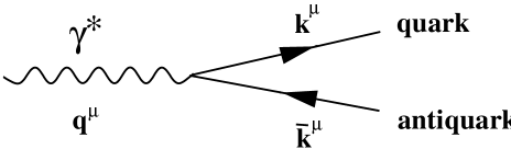
Fig. 5.6: Decomposition of a virtual photon into a quark-antiquark pair at large $Q^{2}$.

It is useful to perform the two-dimensional Fourier transform with respect to the transverse quark momentum $\mathchoice{\mbox{\boldmath$k$}}{\mbox{\boldmath$k$}}{\kern-0.20004pt\hbox{$\scriptstyle k$}\kern-3.86458pt\kern 0.39993pt\hbox{$\scriptstyle k$}\kern-3.86458pt\kern-0.20004pt\raise 0.21698pt\hbox{$\scriptstyle k$}}{\kern-0.20004pt\hbox{$\scriptscriptstyle k$}\kern-2.7604pt\kern 0.39993pt\hbox{$\scriptscriptstyle k$}\kern-2.7604pt\kern-0.20004pt\raise 0.21698pt\hbox{$\scriptscriptstyle k$}}_{\perp}$ conjugate to the transverse separation $b$ of the $q\bar{q}$ pair. Neglecting the quark mass at large $Q^{2}$ and using generically one single quark flavor, the squared wave function of the $q\bar{q}$ component coupled to the longitudinally polarized photon becomes [161, 162, 163]:

$$\left|\psi_{q\bar{q}}^{L}(b,\xi;Q^{2})\right|^{2}=\frac{6\alpha}{\pi^{2}}\,Q^{2}\xi^{2}(1-\xi)^{2}\,K_{0}^{2}\left(b\,Q\,\sqrt{\xi(1-\xi)}\right),$$ (5.29)

where $K_{n}$ denotes modified Bessel functions. The $\gamma^{*}\rightarrow q\bar{q}$ coupling is proportional to the fine structure constant $\alpha\simeq 1/137$. The corresponding result for a virtual photon with transverse polarization is:

$$\left|\psi_{q\bar{q}}^{T}(b,\xi;Q^{2})\right|^{2}=\frac{3\alpha}{2\pi^{2}}\,Q^{2}\xi(1-\xi)\left(\xi^{2}+(1-\xi)^{2}\right)K_{1}^{2}\left(b\,Q\,\sqrt{\xi(1-\xi)}\right).$$ (5.30)

Consider now DIS from a free nucleon at small Bjorken-$x$ and large $Q^{2}$. At the high energies involved the photon in the laboratory frame acts like a beam of $q\bar{q}$ pairs, and one can write the cross section for the longitudinally or transversely polarized virtual photon with the nucleon in the form [162, 164]

$$\sigma_{\gamma^{*}{\mathrm{N}}}^{L,T}=\intop d^{2}b\,\intop_{0}^{1}d\xi\,\left|\psi_{q\bar{q}}^{L,T}(b,\xi)\right|^{2}\,\sigma_{q\bar{q}{{\mathrm{N}}}}(b,x),$$ (5.31)

using the wave functions of the leading $q\bar{q}$ fluctuations. These wave functions as well as the $q\bar{q}$-nucleon cross section $\sigma_{q\bar{q}{{\mathrm{N}}}}$ depend on the transverse separation $b$ of the quark pair. Since the modified Bessel functions in Eqs.(5.29, 5.30) drop as $K_{1,0}(y)\rightarrow e^{-y}$ at large $y$, the wave functions $\psi_{q\bar{q}}^{L,T}$ receive their dominant contributions from configurations with transverse size

$$b^{2}\sim\frac{1}{Q^{2}\,\xi\,(1-\xi)}\,.$$ (5.32)

Consequently, $q\bar{q}$ configurations at large $Q^{2}$ with comparable momenta of the quark and antiquark, $\xi\sim 1-\xi\sim 1/2$, have small transverse size, $b^{2}\sim 1/k_{\perp}^{2}\sim 1/Q^{2}$, or equivalently, large transverse momentum. The interaction of these “non-aligned” configurations with the nucleon is therefore determined by the short transverse distance behavior of the cross section $\sigma_{q\bar{q}{{\mathrm{N}}}}$ which can be calculated using perturbative QCD. The reasoning goes as follows. At large $Q^{2}$ the leading mechanism responsible for the short distance interaction of the $q\bar{q}$ pair with the nucleon is two-gluon exchange (see Fig.5.7). The (color singlet) $q\bar{q}$ pair acts as a color dipole. Its interaction strength with the nucleon or any other (color singlet) hadron is determined by the squared color dipole moment, hence $\sigma_{q\bar{q}{{\mathrm{N}}}}$ is proportional to $b^{2}$ for small transverse separations $b$. In the leading-logarithmic approximation valid at large $Q^{2}$ one derives [164, 165]

$$\sigma_{q\bar{q}{{\mathrm{N}}}}(b,x)=\frac{\pi^{2}}{3}\alpha_{s}(Q^{2})\,b^{2}\,x\,g_{{\mathrm{N}}}(x,Q^{2}),$$ (5.33)

with the strong coupling constant $\alpha_{s}$. The $Q^{2}$ scale in (5.33) is set by $Q^{2}\sim 1/b^{2}$. All non-perturbative effects are incorporated in the gluon distribution $g_{{\mathrm{N}}}(x,Q^{2})$ of the target nucleon.

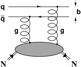
Fig. 5.7: Short distance interaction of a color singlet quark-antiquark pair with a nucleon through two-gluon exchange.

Small $q\bar{q}$ configurations interact only weakly according to Eq.(5.33). This is the case for the kinematic conditions realized in fixed target experiments at CERN and FNAL (see Sections 2.6.1 and 3.3.1). The situation is different at $x\ll 0.1$ and $Q^{2}\gg 1\,\rm{GeV^{2}}$, the extreme region accessible at HERA. Here the strong increase of the nucleon structure function $F_{2}^{{\mathrm{N}}}$ at very small $x$ is accompanied by a correspondingly strong increase of the gluon distribution function. The gluon density becomes so large with decreasing $x$ that, even for small $b^{2}\sim 1/Q^{2}$, the cross section $\sigma_{q\bar{q}{{\mathrm{N}}}}$ can eventually reach magnitudes typical for ordinary hadrons [166].

If either the quark or the antiquark becomes soft (that is: if either the momentum fraction $\xi$ or $1-\xi$ tends to zero), large $q\bar{q}$ separations contribute to the wave functions (5.29, 5.30). In this limit perturbative QCD is not applicable. The interaction cross section for such large-size configurations with small transverse momentum is supposed to be similar to typical hadron-nucleon cross sections [167].

A detailed analysis of the “transverse” wave function (5.30) shows that both “small” (non-aligned) and “large” quark-antiquark configurations give leading $1/Q^{2}$ contributions to the transverse photon-nucleon cross section in accordance with our previous discussion. The situation is different for longitudinally polarized photons (see e.g. (5.29)). In this case the contributions from “soft” quarks (with $\xi\rightarrow 0$ or $1-\xi\rightarrow 0$) are suppressed as $1/Q^{4}$ so that, to leading order in the strong coupling $\alpha_{s}$, only small size $q\bar{q}$ pairs contribute to $\sigma_{\gamma^{*}{\mathrm{N}}}^{L}$. At next to leading order in $\alpha_{s}$, the Fock expansion (5.26) introduces quark-antiquark-gluon states. Large size $q\bar{q}g$ configurations are now important, and they are not suppressed by additional powers of $1/Q^{2}$ [168].

At small momentum transfers, $Q^{2}\mathrel{\raise 2.58334pt\hbox{$<$}\kern-7.7778pt\lower 2.79857pt\hbox{$\sim$}}1\,\rm{GeV^{2}}$, configurations of large size dominate the $q\bar{q}$ wave function. Strong interactions between quark and antiquark now lead to the formation of soft hadronic fluctuations including vector mesons and multi-pion states. Consequently, photon-nucleon cross sections at small $x$ and small $Q^{2}$ receive important contributions from the low mass vector mesons. For example, at $Q^{2}\simeq 0.5$ GeV² almost half of the measured nucleon structure function $F_{2}^{{\mathrm{N}}}$ comes from $\rho,\omega$ and $\phi$ mesons according to the calculation in Ref.[169].

So far we have focused this discussion on free nucleons. Similar considerations apply to deep-inelastic scattering from nuclei which involves the interaction of hadronic components of the virtual photon with the nuclear many-body system. To leading order in $\alpha_{s}$ the photon-nucleus cross sections are now obtained from Eq.(5.31) replacing $\sigma_{q\bar{q}{\mathrm{N}}}$ by the corresponding $q\bar{q}$-nucleus cross section $\sigma_{q\bar{q}{\mathrm{A}}}$. The cross section $\sigma_{{\mathrm{hA}}}$ of any hadronic fluctuation ${\mathrm{h}}$ interacting with a nucleus at high energies, can be related to the cross section for the scattering from free nucleons by the Glauber-Gribov multiple scattering formalism [149, 150]. For a Gaussian nuclear density (5.20) this leads to:

$$\sigma_{{\mathrm{hA}}}\approx A\,\sigma_{{\mathrm{hN}}}\left[1-\sigma_{{\mathrm{hN}}}\,\frac{3}{16\pi}\,\frac{A-1}{\langle r^{2}\rangle_{{\mathrm{A}}}}\,\exp\left(-\frac{\langle r^{2}\rangle_{{\mathrm{A}}}}{3\,\lambda^{2}}\right)+\dots\right],$$ (5.34)

where $\lambda$ is the propagation length associated with the hadronic fluctuation. Double scattering gives a negative correction proportional to the squared cross section of the hadronic fluctuation. Only those hadronic configurations with large interaction cross sections contribute significantly to shadowing. Furthermore, since the nuclear mean square radius behaves approximately as $\langle r^{2}\rangle_{{\mathrm{A}}}\sim A^{2/3}$, the magnitude of the double scattering correction grows for large nuclei with the radius of the target, i.e. proportional to $A^{1/3}$. The exponential in (5.34) ensures that only hadronic fluctuations with propagation lengths $\lambda$ larger than the target dimension contribute significantly to shadowing. For small-sized fluctuations, interesting effects beyond those covered by Eq.(5.34) arise from diffractive production on the whole nucleus.

In accordance with our discussion in the previous section we can conclude:

• In the fixed target experiments at CERN and FNAL, where small values of $x<0.01$ are accessible only at small average momentum transfers, $\overline{Q}\,^{2}\mathrel{\raise 2.58334pt\hbox{$<$}\kern-7.7778pt\lower 2.79857pt\hbox{$\sim$}}1$ GeV², nuclear shadowing is governed by interactions of configurations with large transverse sizes. Contributions from the vector mesons $\rho,\omega$ and $\phi$ turn out to be particularly important.

• At very small $x$ together with very large $Q^{2}$, the growing number of partons in the photon-nucleus system makes them interact like ordinary hadrons, even if the parton configurations have small transverse sizes inversely proportional to $Q^{2}$. One now expects a complex interplay between soft (large-size) and hard (small-size) partonic components of the interacting photon which can no longer be classified by simple book-keeping in powers of $1/Q^{2}$.

5.4 Models

In the following we sketch several models which have been used quite successfully to describe nuclear shadowing as measured in experiments at CERN and FNAL. As before we restrict ourselves to lab-frame descriptions. We do not aim for completeness but rather emphasize common features of various models and their implications for the underlying mechanism of nuclear shadowing.

5.4.1 Vector mesons and aligned jets

As discussed in Section 5.3, the quark-antiquark fluctuation of a virtual photon starts out with a transverse size $b^{2}\sim[Q^{2}\xi(1-\xi)]^{-1}$ where $\xi$ is the fraction of longitudinal photon momentum carried by one of the quarks. “Non-Aligned” $q\bar{q}$ configurations with $\xi\simeq 1/2$ have small transverse size and interact weakly; “aligned” ones with $\xi\sim 0$ or $\xi\sim 1$ have large transverse size and are likely, by subsequent strong interactions, to turn into vector mesons if the $q\bar{q}$ invariant mass matches appropriately.

Models which combine aspects of vector meson dominance and the aligned-jet picture [167] are described in Refs.[169, 170]. Their starting point is the hadronic spectrum of the virtual photon exchanged in the deep-inelastic scattering process. The spectral function, $\mathchar 5\relax(s)$, is determined by the cross section for electron-positron annihilation into hadrons, where $s=q^{2}$ is the squared photon or $e^{+}e^{-}$ center-of-mass energy:

$$\mathchar 5\relax(s)=\frac{1}{12\,\pi^{2}}\frac{\sigma_{e^{+}e^{-}\rightarrow hadrons}(s)}{\sigma_{e^{+}e^{-}\rightarrow\mu^{+}\mu^{-}}(s)}\,,$$ (5.35)

with

$$\mathchar 5\relax(q^{2})=-\frac{1}{3\,q^{2}}\sum_{{\mathrm{X}}}(2\pi)^{3}\delta^{4}(q-p_{{\mathrm{X}}})\left\langle 0\right|J_{\mu}(0)\left|{{\mathrm{X}}}\right\rangle\left\langle{{\mathrm{X}}}\right|J^{\mu}(0)\left|0\right\rangle.$$ (5.36)

Here $J^{\mu}$ is the electromagnetic current operator. The sum in Eq.(5.36) is taken over all hadronic fluctuations of the photon with four-momenta $p_{{\mathrm{X}}}=q$ and squared invariant masses $\mu^{2}\equiv p_{{\mathrm{X}}}^{2}=q^{2}$. At small center-of-mass energies, $s\,\mathrel{\raise 2.58334pt\hbox{$<$}\kern-7.7778pt\lower 2.79857pt\hbox{$\sim$}}\,1$GeV², the spectrum (5.36) is dominated by the vector mesons $\rho$, $\omega$ and $\phi$ as shown in Fig.5.8. The high energy spectrum at $s>1$ GeV² is characterized by quark-antiquark continuum plateaus together with isolated charmonium and upsilon resonances.

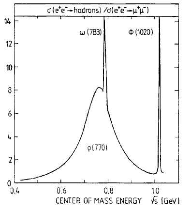
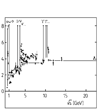
Fig. 5.8: Cross section $\sigma_{e^{+}e^{-}\rightarrow{{\mathrm{hadrons}}}}/\sigma_{e^{+}e^{-}\rightarrow\mu^{+}\mu^{-}}$.

The lab frame space-time pattern of deep-inelastic scattering (Section 4) suggests that the nucleon structure function at small $x$ can be described by the following expression [149, 170]:

$$F_{2}^{{\mathrm{N}}}(x,Q^{2})=\frac{Q^{2}}{\pi}\intop_{4m_{\pi}^{2}}^{\mu_{max}^{2}}\,d\mu^{2}\,\frac{\mu^{2}\,\mathchar 5\relax(\mu^{2})}{\left(\mu^{2}+Q^{2}\right)^{2}}\;\intop_{0}^{1}\,d\xi\,\sigma_{{\mathrm{hN}}}(W,\mu^{2};\xi)\,.$$ (5.37)

The basic idea behind this ansatz is the following. For $x\ll 1$, or large lab frame propagation length $\lambda\sim 2\nu/(Q^{2}+\mu^{2})$ of a given $q\bar{q}$ fluctuation of mass $\mu$, the vacuum spectrum $\mathchar 5\relax(\mu^{2})$ remains more or less unaffected by the presence of the target nucleon. The high-energy virtual photon with $\nu\gg Q^{2}/2M$ behaves like a beam of hadrons with masses $\mu<\mu_{\max}$. Their maximum possible mass is determined by the condition that $\lambda$ must exceed the size $R\simeq 5M^{-1}$ of the target nucleon, so that (roughly) $\mu_{\max}\sim\sqrt{\nu M}$. The interaction of this beam with the nucleon is described by the cross section $\sigma_{{\mathrm{hN}}}$ which depends on $\mu^{2}$ and on the hadron/photon-nucleon center-of-mass energy $W=\sqrt{2M\nu+M^{2}-Q^{2}}\simeq\sqrt{2M\nu}=Q/\sqrt{x}$. For a $q\bar{q}$ pair treated to leading order in $\alpha_{s}$, it also depends on the fraction $\xi$ of the photon light-cone momentum carried by the quark. The sum in Eq.(5.37) is taken over hadronic fluctuations of the photon with fixed invariant mass. The ansatz neglects contributions to the forward virtual photon scattering amplitude in which the mass $\mu$ can change during the interaction.

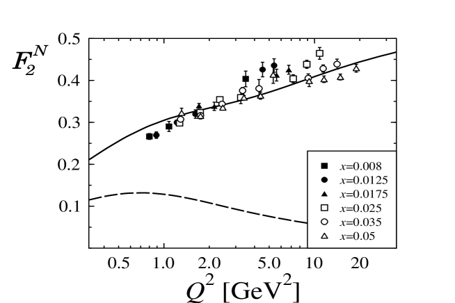
Fig. 5.9: The nucleon structure function $F_{2}^{{\mathrm{N}}}$ for small $x$ plotted against $Q^{2}$. The full line has been obtained in Ref.[169] from Eq.(5.37). The dashed line indicates the contribution of the vector mesons $\rho$, $\omega$ and $\phi$. The data are from the NMC [171].

The small-$x$ structure function $F_{2}^{{\mathrm{N}}}(x,Q^{2})$ as given in Eq.(5.37) is governed by contributions from intermediate hadronic states with an invariant mass $\mu^{2}\sim Q^{2}$. For small momentum transfers, $Q^{2}\,\mathrel{\raise 2.58334pt\hbox{$<$}\kern-7.7778pt\lower 2.79857pt\hbox{$\sim$}}\,1\,\mbox{GeV}^{2}$, low mass vector mesons $\rho,\;\omega$ and $\phi$ are of major importance. Their dominance leads to the scale breaking behavior $F_{2}^{{\mathrm{N}}}(x,Q^{2})\sim Q^{2}$ for $Q^{2}\rightarrow 0$ at small $x$.

For larger momentum transfers, $Q^{2}>m_{\phi}^{2}\approx 1\,\mbox{GeV}^{2}$, the structure function $F_{2}^{{\mathrm{N}}}$ is determined primarily by the interactions of quark-antiquark pairs from the ${q\bar{q}}$ continuum. The color singlet nature of hadronic fluctuations of the virtual photon implies that their interaction cross section is proportional to their transverse size. Quark pairs with momenta “aligned” along the direction of the virtual photon have a large transverse size. Their cross sections should be comparable to typical hadronic cross sections. On the other hand “non-aligned” quarks are characterized by small transverse size. Their cross sections should therefore be small.

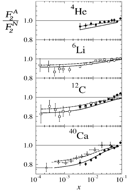
Fig. 5.10: Results from Ref.[169] for the shadowing in He, Li, C, and Ca compared to experimental data from NMC (dots and squares) [71, 75] and FNAL (triangles) [77]. The dashed curves show the shadowing caused by the vector mesons $\rho$, $\omega$ and $\phi$ only, the solid curves are the results including the $q\bar{q}$ continuum.

With these ingredients, Eq.(5.37) gives a good description of the free nucleon structure function $F_{2}^{{\mathrm{N}}}$ for $x<0.1$ and moderate $Q^{2}$. A comparison with data from NMC is shown in Fig.5.9. While the vector meson contribution vanishes as $1/Q^{2}$ for large $Q^{2}$, the ${q\bar{q}}$ continuum pairs are responsible for scaling, $F_{2}^{{\mathrm{N}}}(x,Q^{2})\sim\ln(Q^{2})$, at large $Q^{2}$. Note however the importance of vector mesons at small $Q^{2}$. One finds that at $Q^{2}=1\,\mbox{GeV}^{2}$ almost half of $F_{2}^{{\mathrm{N}}}$ at $x=0.01$ is due to vector mesons. At $Q^{2}=10\,\mbox{GeV}^{2}$ they still contribute about $15\%$. In these calculations the vector meson part of the spectrum $\mathchar 5\relax(\mu^{2})$ is [25]:

$$\mathchar 5\relax^{({\mathrm{V}})}(\mu^{2})=\left(\frac{m_{V}}{g_{V}}\right)^{2}\delta(\mu^{2}-m_{V}^{2})$$ (5.38)

with $V=\rho,\omega,\phi$, the empirical vector meson masses $m_{{\mathrm{V}}}$ and the coupling constants $g_{\rho}=5.0$, $g_{\omega}=17.0$ and $g_{\phi}=12.9$. The vector meson-nucleon cross sections are $\sigma_{\rho{\mathrm{N}}}\approx\sigma_{\omega{\mathrm{N}}}\approx 25$ mb, $\sigma_{\phi{\mathrm{N}}}\approx 10$ mb.

Nuclear structure functions $F_{2}^{{\mathrm{A}}}$ for $x<0.1$ are expressed in an analogous way as in Eq.(5.37), with the hadron-nucleon cross sections $\sigma_{{\mathrm{hN}}}$ replaced by the corresponding hadron-nucleus cross sections $\sigma_{{\mathrm{hA}}}$. The relation between $\sigma_{{\mathrm{hA}}}$ and $\sigma_{{\mathrm{hN}}}$ is given by Glauber-Gribov multiple scattering theory, see Eq.(5.34). In Fig.5.10 we present typical results for the shadowing ratio $R_{{\mathrm{A}}}=F_{2}^{{\mathrm{A}}}/F_{2}^{{\mathrm{N}}}$ from Ref.[169].

Finally we comment on the observed weak $Q^{2}$-dependence of the shadowing effect. In the spectral ansatz (5.37) the given value of $Q^{2}$ selects that part of the hadron mass spectrum around $\mu^{2}\sim Q^{2}$ which dominates the interaction, and hence determines which cross sections $\sigma_{{\mathrm{hN}}}(\mu^{2})$ contribute significantly to the multiple scattering series. While the interaction cross sections decrease as $1/\mu^{2}$ with increasing mass as required by Bjorken scaling, pairs which are aligned with the photon momentum interact with large cross sections, even for large $\mu$, and therefore produce strong shadowing. This is the reason for the very weak overall $Q^{2}$-dependence of shadowing in this framework. A comparison of results from Ref.[169] with NMC data for the slope $b$ of the ratio $F_{2}^{{\mathrm{Sn}}}/F_{2}^{{\mathrm{C}}}\approx a+b\ln Q^{2}$ is presented in Fig.5.11. For a more detailed discussion of these issues including QCD corrections, see Ref.[1].

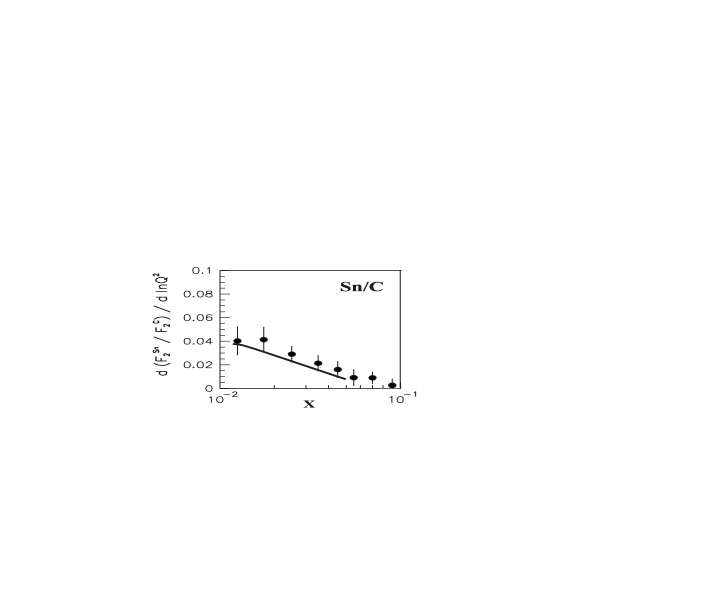
Fig. 5.11: The slope $b=d(F_{2}^{{\mathrm{Sn}}}/F_{2}^{{\mathrm{C}}})/d\ln Q^{2}$ indicating the $Q^{2}$ dependence of the shadowing ratio ${\mathrm{Sn}}/{{\mathrm{C}}}$. The calculation is described in [169]. Data are taken from [82].

5.4.2 Vector meson dominance and pomeron exchange

As indicated in Eqs.(5.11,5.18), nuclear shadowing is directly related to the diffractive production cross section $d\sigma^{diff}_{\gamma^{*}{{\mathrm{N}}}}/dM_{{\mathrm{X}}}^{2}\,dt$ or, equivalently, to the diffractive structure function $F_{2}^{D(4)}$.

Diffractive production at $Q^{2}\,\mathrel{\raise 2.58334pt\hbox{$<$}\kern-7.7778pt\lower 2.79857pt\hbox{$\sim$}}\,1\,\rm{GeV}^{2}$ is dominated by the excitation of the vector mesons $\rho$, $\omega$ and $\phi$. Their contributions can be described within the framework of vector meson dominance (see e.g. [25]). Neglecting transitions between different vector mesons and omitting contributions from longitudinally polarized virtual photons one finds:

$$\left.\frac{d\sigma^{diff\,({{\mathrm{V}}})}_{\gamma^{*}{{\mathrm{N}}}}}{dM_{{\mathrm{X}}}^{2}dt}\right|_{t\approx 0}=\frac{\alpha}{4}\,\frac{\mathchar 5\relax^{({\mathrm{V}})}(M_{{\mathrm{X}}}^{2})\,M_{{\mathrm{X}}}^{2}}{(Q^{2}+M_{{\mathrm{X}}}^{2})^{2}}\,\sigma_{{{\mathrm{XN}}}}^{2}\,.$$ (5.39)

Here the vector meson part (5.38) of the photon spectral function enters. Combining Eqs.(5.18,5.39) shows that the contribution of vector mesons to nuclear shadowing vanishes indeed as $1/Q^{2}$.

The diffractive excitation of heavy mass states is commonly parametrized according to the Regge ansatz as in Eq.(2.73). Most descriptions concentrate on the dominant contribution from pomeron exchange. The pomeron structure function $F_{2}^{\rm I\!P}$ is modeled in agreement with available data on diffraction. At large $Q^{2}$ it is supposed to scale, i.e. it depends at most logarithmically on $Q^{2}$. This leads to scaling for nuclear shadowing at large $Q^{2}$. On the other hand, at $Q^{2}\ll 1\,\rm{GeV}^{2}$ one assumes $F_{2}^{\rm I\!P}\sim Q^{2}$ [172] which ensures that the shadowing correction to the nuclear structure function, $\delta F_{2}^{{\mathrm{A}}}$, vanishes at $Q^{2}=0$, just like $F_{2}^{{\mathrm{A}}}$ itself. Investigations of shadowing effects along theses lines can be found in [154, 172, 173, 174, 175, 176]. In Fig.5.12 a typical result for shadowing in ${\mathrm{Xe}}$ from [154] is shown.

Fig. 5.12: Shadowing in ${\mathrm{Xe}}$. Details of the calculation are given in Ref.[154]. The dashed curve shows the contribution of vector mesons $\rho$, $\omega$ and $\phi$, while the solid curve includes pomeron exchange. The data are from the E665 collaboration [76].

5.4.3 Generalized vector meson dominance

Generalized vector meson dominance models describe deep-inelastic lepton scattering at small $x$ purely in terms of hadronic degrees of freedom [177, 178, 179, 180, 181, 182, 183, 184, 185]. For a free nucleon this leads to the following picture: prior to its interaction with the target the virtual photon fluctuates into a hadronic state with invariant mass $\mu$. This fluctuation scatters from the target and converts into a hadronic state with mass $\mu^{\prime}$. For transversely polarized photons this translates into a forward Compton amplitude of the form:

$${\cal A}_{\gamma^{*}{{\mathrm{N}}}}^{T}(W,Q^{2})\sim\intop d\,\mu^{2}\intop d{\mu^{\prime}}^{2}\frac{\rho(\mu,\mu^{\prime};W)}{(\mu^{2}+Q^{2})({\mu^{\prime}}^{2}+Q^{2})}\,,$$ (5.40)

with a double spectral distribution $\rho$ depending on the photon-nucleon center-of-mass energy $W$. Here the integrals over initial and final hadronic fluctuations and their propagators are made explicit.

The continuum of hadronic intermediate states which determines the double spectral function $\rho(\mu,\mu^{\prime};W)$ is commonly approximated by a discrete set of narrow vector meson states ${{\mathrm{V}}}_{n}$ $(n=1,2,\dots)$. The resulting transverse photon-nucleon cross section is:

$$\sigma^{T}_{\gamma^{*}{{\mathrm{N}}}}=\sum_{n,m}\frac{e}{g_{m}}\frac{M^{2}_{m}}{M^{2}_{m}+Q^{2}}\mathchar 6\relax_{mn}(W)\frac{M^{2}_{n}}{M^{2}_{n}+Q^{2}}\frac{e}{g_{n}}\,.$$ (5.41)

In Refs.[180, 184] the vector mesons are assumed to be equally spaced in mass, starting with the $\rho$-meson. The photon-vector meson couplings $g_{n}$ are chosen to reproduce average scaling in $e^{+}e^{-}$ annihilation into hadrons (see Fig.5.8). $\mathchar 6\relax_{mn}$ denotes the imaginary part of the vector meson-nucleon transition amplitude, ${{\mathrm{V}}}_{m}{{\mathrm{N}}}\rightarrow{{\mathrm{V}}}_{n}{\mathrm{N}}$, in the forward direction. For diagonal terms it is equal to the total ${{\mathrm{V}}}_{n}$-nucleon cross section, $\mathchar 6\relax_{nn}=\sigma({{{\mathrm{V}}}_{n}{\mathrm{N}}})$, which is taken to be constant.

The next step in simplification is to consider only diagonal ($m=n)$ and nearest off-diagonal ($m=n\pm 1$) contributions. A fine-tuned cancelation between the corresponding amplitudes $\mathchar 6\relax_{mn}$ leads to a reasonable description of the nucleon structure function $F_{2}^{{\mathrm{N}}}$ at moderate momentum transfers $Q^{2}$.

An extension of this approach to nuclear targets involves multiple scattering of hadronic fluctuations from several nucleons. The multiple scattering process is described by a coupled channel optical model [179, 184] which accounts for the shadowing criteria in Eq.(5.2), i.e. only those hadronic fluctuations with longitudinal interaction lengths larger than their mean free path in the nuclear medium contribute significantly to multiple scattering and thus to shadowing.

GVMD calculations applied to nuclear DIS data can be found in Refs.[186, 187].

5.4.4 Vector mesons and quark scattering

We add a few remarks and references about approaches dealing with DIS in terms of quark dynamics.

The starting point in Ref.[188] is a description of DIS from nucleons at large $Q^{2}$ and small $x$ in terms of quark-nucleon scattering [189]. The quark-nucleon scattering amplitude is formulated using Regge phenomenology and constrained by the quark distributions of free nucleons. The interaction strength of quark-nucleon scattering is determined by the quark-nucleon cross section, taken to be about $1/3$ of the nucleon-nucleon cross section. At center of mass energies $s\sim 200$ GeV² one finds $\sigma_{q{\mathrm{N}}}\approx 13$ mb [190].

An extension to DIS from nuclei at small $x$ involves the quark-nucleus scattering amplitude. Its connection with the amplitude for the scattering from free nucleons is given through the Glauber-Gribov multiple scattering series.

In Ref.[190] the interactions of strongly correlated quark-antiquark pairs, i.e. vector mesons, have been added. One finds that vector mesons carry more than half of the shadowing effect measured at E665 and NMC. On the other hand, the interaction of uncorrelated quarks is also important to ensure a weak $Q^{2}$-dependence of shadowing.

5.4.5 Green function methods

The previously mentioned models have outlined in different ways the ingredients needed in order to understand the physics of shadowing: the mass spectrum of quark-gluon fluctuations of the virtual photon, and the dynamics of the expanding and strongly interacting quark-gluon configurations in the surrounding nuclear system. In most of the models the longitudinal propagation of hadronic fluctuations of the photon is treated by multiple scattering theory, while the transverse degrees of freedom are more or less “frozen” during the passage through the nucleus. Several questions are faced in this context. The transverse size of quark-gluon fluctuations needs to be connected with their effective mass; the relationship with diffractive production must be elucidated; higher order terms in the multiple scattering series must be systematically incorporated, at least for heavy nuclei.

A coordinate space Green function method which permits to unify all those aspects has been developed in Refs.[191, 192]. This work considers only quark-antiquark fluctuations of the photon. It turns out that some previous approximations can be recovered as limiting cases. We follow Ref.[191] and give here a brief summary of the essentials.

Consider the scattering of a virtual photon with high energy $\nu$ and large squared four-momentum, $Q^{2}>1$ GeV², through a nucleus as illustrated in Fig.5.13. The longitudinal ($z$-) direction is defined by the photon three-momentum, as usual. At point $z_{1}$ the photon produces a quark-antiquark pair with transverse separation $b_{1}$. Along its passage to point $z_{2}$ where it has a transverse separation $b_{2}$, the $q\bar{q}$ fluctuation experiences multiple interactions with nucleons in the nuclear target. We are interested in the full Green function $G(\mathchoice{\mbox{\boldmath$b$}}{\mbox{\boldmath$b$}}{\kern-0.20004pt\hbox{$\scriptstyle b$}\kern-3.00417pt\kern 0.39993pt\hbox{$\scriptstyle b$}\kern-3.00417pt\kern-0.20004pt\raise 0.21698pt\hbox{$\scriptstyle b$}}{\kern-0.20004pt\hbox{$\scriptscriptstyle b$}\kern-2.14583pt\kern 0.39993pt\hbox{$\scriptscriptstyle b$}\kern-2.14583pt\kern-0.20004pt\raise 0.21698pt\hbox{$\scriptscriptstyle b$}}_{2},z_{2};\mathchoice{\mbox{\boldmath$b$}}{\mbox{\boldmath$b$}}{\kern-0.20004pt\hbox{$\scriptstyle b$}\kern-3.00417pt\kern 0.39993pt\hbox{$\scriptstyle b$}\kern-3.00417pt\kern-0.20004pt\raise 0.21698pt\hbox{$\scriptstyle b$}}{\kern-0.20004pt\hbox{$\scriptscriptstyle b$}\kern-2.14583pt\kern 0.39993pt\hbox{$\scriptscriptstyle b$}\kern-2.14583pt\kern-0.20004pt\raise 0.21698pt\hbox{$\scriptscriptstyle b$}}_{1},z_{1})$ which describes the propagation of the $q\bar{q}$ pair from $z_{1}$ to $z_{2}$, including its dynamics in the transverse space coordinate.

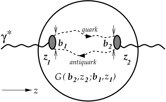
Fig. 5.13: Propagation of a quark-antiquark fluctuation of the virtual photon $\gamma^{*}$ between points $z_{1}$ and $z_{2}$ where the pair has transverse separation $\mathchoice{\mbox{\boldmath$b$}}{\mbox{\boldmath$b$}}{\kern-0.20004pt\hbox{$\scriptstyle b$}\kern-3.00417pt\kern 0.39993pt\hbox{$\scriptstyle b$}\kern-3.00417pt\kern-0.20004pt\raise 0.21698pt\hbox{$\scriptstyle b$}}{\kern-0.20004pt\hbox{$\scriptscriptstyle b$}\kern-2.14583pt\kern 0.39993pt\hbox{$\scriptscriptstyle b$}\kern-2.14583pt\kern-0.20004pt\raise 0.21698pt\hbox{$\scriptscriptstyle b$}}_{1}$ and $\mathchoice{\mbox{\boldmath$b$}}{\mbox{\boldmath$b$}}{\kern-0.20004pt\hbox{$\scriptstyle b$}\kern-3.00417pt\kern 0.39993pt\hbox{$\scriptstyle b$}\kern-3.00417pt\kern-0.20004pt\raise 0.21698pt\hbox{$\scriptstyle b$}}{\kern-0.20004pt\hbox{$\scriptscriptstyle b$}\kern-2.14583pt\kern 0.39993pt\hbox{$\scriptscriptstyle b$}\kern-2.14583pt\kern-0.20004pt\raise 0.21698pt\hbox{$\scriptscriptstyle b$}}_{2}$. The Green function $G(\mathchoice{\mbox{\boldmath$b$}}{\mbox{\boldmath$b$}}{\kern-0.20004pt\hbox{$\scriptstyle b$}\kern-3.00417pt\kern 0.39993pt\hbox{$\scriptstyle b$}\kern-3.00417pt\kern-0.20004pt\raise 0.21698pt\hbox{$\scriptstyle b$}}{\kern-0.20004pt\hbox{$\scriptscriptstyle b$}\kern-2.14583pt\kern 0.39993pt\hbox{$\scriptscriptstyle b$}\kern-2.14583pt\kern-0.20004pt\raise 0.21698pt\hbox{$\scriptscriptstyle b$}}_{2},z_{2};\mathchoice{\mbox{\boldmath$b$}}{\mbox{\boldmath$b$}}{\kern-0.20004pt\hbox{$\scriptstyle b$}\kern-3.00417pt\kern 0.39993pt\hbox{$\scriptstyle b$}\kern-3.00417pt\kern-0.20004pt\raise 0.21698pt\hbox{$\scriptstyle b$}}{\kern-0.20004pt\hbox{$\scriptscriptstyle b$}\kern-2.14583pt\kern 0.39993pt\hbox{$\scriptscriptstyle b$}\kern-2.14583pt\kern-0.20004pt\raise 0.21698pt\hbox{$\scriptscriptstyle b$}}_{1},z_{1})$ sums all possible paths of the pair through the nucleus.

This Green function enters in the shadowing part of the $\gamma^{*}$-nucleus cross section, as follows. One writes:

$$\delta\sigma_{\gamma^{*}{\mathrm{A}}}(x,Q^{2}) \equiv \sigma_{\gamma^{*}{\mathrm{A}}}(x,Q^{2})-A\,\sigma_{\gamma^{*}{\mathrm{N}}}(x,Q^{2})$$ (5.42)

$$= -2\intop d^{2}b\intop_{-\infty}^{\infty}dz_{1}\,\rho_{{\mathrm{A}}}(\mathchoice{\mbox{\boldmath$b$}}{\mbox{\boldmath$b$}}{\kern-0.20004pt\hbox{$\scriptstyle b$}\kern-3.00417pt\kern 0.39993pt\hbox{$\scriptstyle b$}\kern-3.00417pt\kern-0.20004pt\raise 0.21698pt\hbox{$\scriptstyle b$}}{\kern-0.20004pt\hbox{$\scriptscriptstyle b$}\kern-2.14583pt\kern 0.39993pt\hbox{$\scriptscriptstyle b$}\kern-2.14583pt\kern-0.20004pt\raise 0.21698pt\hbox{$\scriptscriptstyle b$}},z_{1})\intop_{z_{1}}^{\infty}dz_{2}\,\rho_{{\mathrm{A}}}(\mathchoice{\mbox{\boldmath$b$}}{\mbox{\boldmath$b$}}{\kern-0.20004pt\hbox{$\scriptstyle b$}\kern-3.00417pt\kern 0.39993pt\hbox{$\scriptstyle b$}\kern-3.00417pt\kern-0.20004pt\raise 0.21698pt\hbox{$\scriptstyle b$}}{\kern-0.20004pt\hbox{$\scriptscriptstyle b$}\kern-2.14583pt\kern 0.39993pt\hbox{$\scriptscriptstyle b$}\kern-2.14583pt\kern-0.20004pt\raise 0.21698pt\hbox{$\scriptscriptstyle b$}},z_{2})\,W(z_{2},z_{1}).$$

The quantity $W(z_{2},z_{1})$ has dimension $(length)^{4}$ and describes the production of a $q\bar{q}$ fluctuation in the process $\gamma^{*}{\mathrm{N}}\rightarrow q\bar{q}\,{\mathrm{N}}$, its propagation from $z_{1}$ to $z_{2}$, and its subsequent conversion back to a virtual photon:

$$W(z_{2},z_{1})=Re\,\intop d^{2}b_{1}\intop d^{2}b_{2}\intop_{0}^{1}d\xi\,{\cal F}^{*}(\mathchoice{\mbox{\boldmath$b$}}{\mbox{\boldmath$b$}}{\kern-0.20004pt\hbox{$\scriptstyle b$}\kern-3.00417pt\kern 0.39993pt\hbox{$\scriptstyle b$}\kern-3.00417pt\kern-0.20004pt\raise 0.21698pt\hbox{$\scriptstyle b$}}{\kern-0.20004pt\hbox{$\scriptscriptstyle b$}\kern-2.14583pt\kern 0.39993pt\hbox{$\scriptscriptstyle b$}\kern-2.14583pt\kern-0.20004pt\raise 0.21698pt\hbox{$\scriptscriptstyle b$}}_{2},\xi)\,G(\mathchoice{\mbox{\boldmath$b$}}{\mbox{\boldmath$b$}}{\kern-0.20004pt\hbox{$\scriptstyle b$}\kern-3.00417pt\kern 0.39993pt\hbox{$\scriptstyle b$}\kern-3.00417pt\kern-0.20004pt\raise 0.21698pt\hbox{$\scriptstyle b$}}{\kern-0.20004pt\hbox{$\scriptscriptstyle b$}\kern-2.14583pt\kern 0.39993pt\hbox{$\scriptscriptstyle b$}\kern-2.14583pt\kern-0.20004pt\raise 0.21698pt\hbox{$\scriptscriptstyle b$}}_{2},z_{2};\mathchoice{\mbox{\boldmath$b$}}{\mbox{\boldmath$b$}}{\kern-0.20004pt\hbox{$\scriptstyle b$}\kern-3.00417pt\kern 0.39993pt\hbox{$\scriptstyle b$}\kern-3.00417pt\kern-0.20004pt\raise 0.21698pt\hbox{$\scriptstyle b$}}{\kern-0.20004pt\hbox{$\scriptscriptstyle b$}\kern-2.14583pt\kern 0.39993pt\hbox{$\scriptscriptstyle b$}\kern-2.14583pt\kern-0.20004pt\raise 0.21698pt\hbox{$\scriptscriptstyle b$}}_{1},z_{1})\,{\cal F}(\mathchoice{\mbox{\boldmath$b$}}{\mbox{\boldmath$b$}}{\kern-0.20004pt\hbox{$\scriptstyle b$}\kern-3.00417pt\kern 0.39993pt\hbox{$\scriptstyle b$}\kern-3.00417pt\kern-0.20004pt\raise 0.21698pt\hbox{$\scriptstyle b$}}{\kern-0.20004pt\hbox{$\scriptscriptstyle b$}\kern-2.14583pt\kern 0.39993pt\hbox{$\scriptscriptstyle b$}\kern-2.14583pt\kern-0.20004pt\raise 0.21698pt\hbox{$\scriptscriptstyle b$}}_{1},\xi)\,e^{i\kappa(z_{2}-z_{1})}.$$ (5.43)

It involves the amplitude

$${\cal F}(\mathchoice{\mbox{\boldmath$b$}}{\mbox{\boldmath$b$}}{\kern-0.20004pt\hbox{$\scriptstyle b$}\kern-3.00417pt\kern 0.39993pt\hbox{$\scriptstyle b$}\kern-3.00417pt\kern-0.20004pt\raise 0.21698pt\hbox{$\scriptstyle b$}}{\kern-0.20004pt\hbox{$\scriptscriptstyle b$}\kern-2.14583pt\kern 0.39993pt\hbox{$\scriptscriptstyle b$}\kern-2.14583pt\kern-0.20004pt\raise 0.21698pt\hbox{$\scriptscriptstyle b$}},\xi)=\frac{1}{2}\psi_{\gamma^{*}\rightarrow q\bar{q}}(\mathchoice{\mbox{\boldmath$b$}}{\mbox{\boldmath$b$}}{\kern-0.20004pt\hbox{$\scriptstyle b$}\kern-3.00417pt\kern 0.39993pt\hbox{$\scriptstyle b$}\kern-3.00417pt\kern-0.20004pt\raise 0.21698pt\hbox{$\scriptstyle b$}}{\kern-0.20004pt\hbox{$\scriptscriptstyle b$}\kern-2.14583pt\kern 0.39993pt\hbox{$\scriptscriptstyle b$}\kern-2.14583pt\kern-0.20004pt\raise 0.21698pt\hbox{$\scriptscriptstyle b$}},\xi)\,\sigma(\mathchoice{\mbox{\boldmath$b$}}{\mbox{\boldmath$b$}}{\kern-0.20004pt\hbox{$\scriptstyle b$}\kern-3.00417pt\kern 0.39993pt\hbox{$\scriptstyle b$}\kern-3.00417pt\kern-0.20004pt\raise 0.21698pt\hbox{$\scriptstyle b$}}{\kern-0.20004pt\hbox{$\scriptscriptstyle b$}\kern-2.14583pt\kern 0.39993pt\hbox{$\scriptscriptstyle b$}\kern-2.14583pt\kern-0.20004pt\raise 0.21698pt\hbox{$\scriptscriptstyle b$}})$$ (5.44)

for the $\gamma^{*}{\mathrm{N}}\rightarrow q\bar{q}\,{\mathrm{N}}$ process leading to a $q\bar{q}$ pair of transverse separation $b$ in which the quark carries the fraction $\xi$ of the photon light cone momentum (see also Section 5.3). The color dipole cross section $\sigma(\mathchoice{\mbox{\boldmath$b$}}{\mbox{\boldmath$b$}}{\kern-0.20004pt\hbox{$\scriptstyle b$}\kern-3.00417pt\kern 0.39993pt\hbox{$\scriptstyle b$}\kern-3.00417pt\kern-0.20004pt\raise 0.21698pt\hbox{$\scriptstyle b$}}{\kern-0.20004pt\hbox{$\scriptscriptstyle b$}\kern-2.14583pt\kern 0.39993pt\hbox{$\scriptscriptstyle b$}\kern-2.14583pt\kern-0.20004pt\raise 0.21698pt\hbox{$\scriptscriptstyle b$}})$ has the characteristic color screening behavior, i.e. it vanishes as $b^{2}$ at $b\rightarrow 0$ (see also Eq.(5.33)), and the distribution of transverse separations is determined by the amplitude $\psi_{\gamma^{*}\rightarrow q\bar{q}}$. The normalization of $\cal F$ is such that its Fourier transform gives the $\gamma^{*}{\mathrm{N}}\rightarrow q\bar{q}\,{\mathrm{N}}$ diffractive dissociation amplitude,

$$f(\mathchoice{\mbox{\boldmath$k$}}{\mbox{\boldmath$k$}}{\kern-0.20004pt\hbox{$\scriptstyle k$}\kern-3.86458pt\kern 0.39993pt\hbox{$\scriptstyle k$}\kern-3.86458pt\kern-0.20004pt\raise 0.21698pt\hbox{$\scriptstyle k$}}{\kern-0.20004pt\hbox{$\scriptscriptstyle k$}\kern-2.7604pt\kern 0.39993pt\hbox{$\scriptscriptstyle k$}\kern-2.7604pt\kern-0.20004pt\raise 0.21698pt\hbox{$\scriptscriptstyle k$}}_{\perp})=\intop d^{2}b\,{\cal F}(\mathchoice{\mbox{\boldmath$b$}}{\mbox{\boldmath$b$}}{\kern-0.20004pt\hbox{$\scriptstyle b$}\kern-3.00417pt\kern 0.39993pt\hbox{$\scriptstyle b$}\kern-3.00417pt\kern-0.20004pt\raise 0.21698pt\hbox{$\scriptstyle b$}}{\kern-0.20004pt\hbox{$\scriptscriptstyle b$}\kern-2.14583pt\kern 0.39993pt\hbox{$\scriptscriptstyle b$}\kern-2.14583pt\kern-0.20004pt\raise 0.21698pt\hbox{$\scriptscriptstyle b$}},\xi)e^{i\mathchoice{\mbox{\boldmath$k$}}{\mbox{\boldmath$k$}}{\kern-0.14003pt\hbox{$\scriptstyle k$}\kern-2.7052pt\kern 0.27995pt\hbox{$\scriptstyle k$}\kern-2.7052pt\kern-0.14003pt\raise 0.15189pt\hbox{$\scriptstyle k$}}{\kern-0.14003pt\hbox{$\scriptscriptstyle k$}\kern-1.93228pt\kern 0.27995pt\hbox{$\scriptscriptstyle k$}\kern-1.93228pt\kern-0.14003pt\raise 0.15189pt\hbox{$\scriptscriptstyle k$}}_{\perp}\cdot\mathchoice{\mbox{\boldmath$b$}}{\mbox{\boldmath$b$}}{\kern-0.14003pt\hbox{$\scriptstyle b$}\kern-2.1029pt\kern 0.27995pt\hbox{$\scriptstyle b$}\kern-2.1029pt\kern-0.14003pt\raise 0.15189pt\hbox{$\scriptstyle b$}}{\kern-0.14003pt\hbox{$\scriptscriptstyle b$}\kern-1.50208pt\kern 0.27995pt\hbox{$\scriptscriptstyle b$}\kern-1.50208pt\kern-0.14003pt\raise 0.15189pt\hbox{$\scriptscriptstyle b$}}},$$ (5.45)

in plane wave impulse approximation. The phase factor $e^{i\kappa(z_{2}-z_{1})}$ involves the characteristic wave number of the $q\bar{q}$ fluctuation:

$$\kappa=\frac{Q^{2}\,\xi(1-\xi)+m_{q}^{2}}{2\nu\,\xi(1-\xi)}$$ (5.46)

where $m_{q}$ is the (constituent) quark mass. For $\xi=1/2$ the resulting $\kappa=\frac{Q^{2}+4m_{q}^{2}}{2\nu}\equiv\lambda^{-1}$ is just the inverse coherence length of a quark and antiquark which travel side by side. (For arbitrary $\xi$ this coherence length includes the transverse momentum, $\lambda^{-1}=\kappa+\mathchoice{\mbox{\boldmath$k$}}{\mbox{\boldmath$k$}}{\kern-0.20004pt\hbox{$\scriptstyle k$}\kern-3.86458pt\kern 0.39993pt\hbox{$\scriptstyle k$}\kern-3.86458pt\kern-0.20004pt\raise 0.21698pt\hbox{$\scriptstyle k$}}{\kern-0.20004pt\hbox{$\scriptscriptstyle k$}\kern-2.7604pt\kern 0.39993pt\hbox{$\scriptscriptstyle k$}\kern-2.7604pt\kern-0.20004pt\raise 0.21698pt\hbox{$\scriptscriptstyle k$}}_{\perp}/[2\nu\,\xi(1-\xi)]$.)

Let us now return to the propagation function $G$. It satisfies a wave equation [191] which can be made plausible by the following considerations. The longitudinal motion along the $z$-axis is equivalent to the time evolution of the $q\bar{q}$ fluctuation, represented by the operator $i\frac{\partial}{\partial z_{2}}$. The transverse dynamics has a kinetic term,

$$t_{kin}=-\frac{\mathchoice{\mbox{\boldmath$\nabla$}}{\mbox{\boldmath$\nabla$}}{\kern-0.20004pt\hbox{$\scriptstyle\nabla$}\kern-7.49997pt\kern 0.39993pt\hbox{$\scriptstyle\nabla$}\kern-7.49997pt\kern-0.20004pt\raise 0.21698pt\hbox{$\scriptstyle\nabla$}}{\kern-0.20004pt\hbox{$\scriptscriptstyle\nabla$}\kern-5.8333pt\kern 0.39993pt\hbox{$\scriptscriptstyle\nabla$}\kern-5.8333pt\kern-0.20004pt\raise 0.21698pt\hbox{$\scriptscriptstyle\nabla$}}_{b_{2}}^{2}}{2\nu\xi(1-\xi)}$$ (5.47)

with the $2$-dimensional Laplacian acting on the transverse separation coordinate $\mathchoice{\mbox{\boldmath$b$}}{\mbox{\boldmath$b$}}{\kern-0.20004pt\hbox{$\scriptstyle b$}\kern-3.00417pt\kern 0.39993pt\hbox{$\scriptstyle b$}\kern-3.00417pt\kern-0.20004pt\raise 0.21698pt\hbox{$\scriptstyle b$}}{\kern-0.20004pt\hbox{$\scriptscriptstyle b$}\kern-2.14583pt\kern 0.39993pt\hbox{$\scriptscriptstyle b$}\kern-2.14583pt\kern-0.20004pt\raise 0.21698pt\hbox{$\scriptscriptstyle b$}}_{2}$, and the denominator reflecting the effective mass of the pair. Interactions of the $q\bar{q}$ pair with the nuclear medium at an impact parameter $b$ are introduced by an absorptive term,

$$v(b_{2},\mathchoice{\mbox{\boldmath$b$}}{\mbox{\boldmath$b$}}{\kern-0.20004pt\hbox{$\scriptstyle b$}\kern-3.00417pt\kern 0.39993pt\hbox{$\scriptstyle b$}\kern-3.00417pt\kern-0.20004pt\raise 0.21698pt\hbox{$\scriptstyle b$}}{\kern-0.20004pt\hbox{$\scriptscriptstyle b$}\kern-2.14583pt\kern 0.39993pt\hbox{$\scriptscriptstyle b$}\kern-2.14583pt\kern-0.20004pt\raise 0.21698pt\hbox{$\scriptscriptstyle b$}})=-\frac{i}{2}\,\sigma(b_{2})\rho_{{\mathrm{A}}}(\mathchoice{\mbox{\boldmath$b$}}{\mbox{\boldmath$b$}}{\kern-0.20004pt\hbox{$\scriptstyle b$}\kern-3.00417pt\kern 0.39993pt\hbox{$\scriptstyle b$}\kern-3.00417pt\kern-0.20004pt\raise 0.21698pt\hbox{$\scriptstyle b$}}{\kern-0.20004pt\hbox{$\scriptscriptstyle b$}\kern-2.14583pt\kern 0.39993pt\hbox{$\scriptscriptstyle b$}\kern-2.14583pt\kern-0.20004pt\raise 0.21698pt\hbox{$\scriptscriptstyle b$}},z_{2}).$$ (5.48)

The wave equation for $G$ is then of the generic form $i\partial\,G/\partial z=(t_{kin}+v)\,G$ or, more precisely,

$$\left[i\frac{\partial}{\partial z_{2}}+\frac{\mathchoice{\mbox{\boldmath$\nabla$}}{\mbox{\boldmath$\nabla$}}{\kern-0.20004pt\hbox{$\scriptstyle\nabla$}\kern-7.49997pt\kern 0.39993pt\hbox{$\scriptstyle\nabla$}\kern-7.49997pt\kern-0.20004pt\raise 0.21698pt\hbox{$\scriptstyle\nabla$}}{\kern-0.20004pt\hbox{$\scriptscriptstyle\nabla$}\kern-5.8333pt\kern 0.39993pt\hbox{$\scriptscriptstyle\nabla$}\kern-5.8333pt\kern-0.20004pt\raise 0.21698pt\hbox{$\scriptscriptstyle\nabla$}}_{b_{2}}^{2}}{2\nu\,\xi(1-\xi)}+\frac{i}{2}\sigma(b_{2})\,\rho_{{\mathrm{A}}}(\mathchoice{\mbox{\boldmath$b$}}{\mbox{\boldmath$b$}}{\kern-0.20004pt\hbox{$\scriptstyle b$}\kern-3.00417pt\kern 0.39993pt\hbox{$\scriptstyle b$}\kern-3.00417pt\kern-0.20004pt\raise 0.21698pt\hbox{$\scriptstyle b$}}{\kern-0.20004pt\hbox{$\scriptscriptstyle b$}\kern-2.14583pt\kern 0.39993pt\hbox{$\scriptscriptstyle b$}\kern-2.14583pt\kern-0.20004pt\raise 0.21698pt\hbox{$\scriptscriptstyle b$}},z_{2})\right]G(\mathchoice{\mbox{\boldmath$b$}}{\mbox{\boldmath$b$}}{\kern-0.20004pt\hbox{$\scriptstyle b$}\kern-3.00417pt\kern 0.39993pt\hbox{$\scriptstyle b$}\kern-3.00417pt\kern-0.20004pt\raise 0.21698pt\hbox{$\scriptstyle b$}}{\kern-0.20004pt\hbox{$\scriptscriptstyle b$}\kern-2.14583pt\kern 0.39993pt\hbox{$\scriptscriptstyle b$}\kern-2.14583pt\kern-0.20004pt\raise 0.21698pt\hbox{$\scriptscriptstyle b$}}_{2},z_{2};\mathchoice{\mbox{\boldmath$b$}}{\mbox{\boldmath$b$}}{\kern-0.20004pt\hbox{$\scriptstyle b$}\kern-3.00417pt\kern 0.39993pt\hbox{$\scriptstyle b$}\kern-3.00417pt\kern-0.20004pt\raise 0.21698pt\hbox{$\scriptstyle b$}}{\kern-0.20004pt\hbox{$\scriptscriptstyle b$}\kern-2.14583pt\kern 0.39993pt\hbox{$\scriptscriptstyle b$}\kern-2.14583pt\kern-0.20004pt\raise 0.21698pt\hbox{$\scriptscriptstyle b$}}_{1},z_{1})=0$$ (5.49)

with the initial condition $G(\mathchoice{\mbox{\boldmath$b$}}{\mbox{\boldmath$b$}}{\kern-0.20004pt\hbox{$\scriptstyle b$}\kern-3.00417pt\kern 0.39993pt\hbox{$\scriptstyle b$}\kern-3.00417pt\kern-0.20004pt\raise 0.21698pt\hbox{$\scriptstyle b$}}{\kern-0.20004pt\hbox{$\scriptscriptstyle b$}\kern-2.14583pt\kern 0.39993pt\hbox{$\scriptscriptstyle b$}\kern-2.14583pt\kern-0.20004pt\raise 0.21698pt\hbox{$\scriptscriptstyle b$}}_{2},z_{1};\mathchoice{\mbox{\boldmath$b$}}{\mbox{\boldmath$b$}}{\kern-0.20004pt\hbox{$\scriptstyle b$}\kern-3.00417pt\kern 0.39993pt\hbox{$\scriptstyle b$}\kern-3.00417pt\kern-0.20004pt\raise 0.21698pt\hbox{$\scriptstyle b$}}{\kern-0.20004pt\hbox{$\scriptscriptstyle b$}\kern-2.14583pt\kern 0.39993pt\hbox{$\scriptscriptstyle b$}\kern-2.14583pt\kern-0.20004pt\raise 0.21698pt\hbox{$\scriptscriptstyle b$}}_{1},z_{1})=\delta^{2}(\mathchoice{\mbox{\boldmath$b$}}{\mbox{\boldmath$b$}}{\kern-0.20004pt\hbox{$\scriptstyle b$}\kern-3.00417pt\kern 0.39993pt\hbox{$\scriptstyle b$}\kern-3.00417pt\kern-0.20004pt\raise 0.21698pt\hbox{$\scriptstyle b$}}{\kern-0.20004pt\hbox{$\scriptscriptstyle b$}\kern-2.14583pt\kern 0.39993pt\hbox{$\scriptscriptstyle b$}\kern-2.14583pt\kern-0.20004pt\raise 0.21698pt\hbox{$\scriptscriptstyle b$}}_{2}-\mathchoice{\mbox{\boldmath$b$}}{\mbox{\boldmath$b$}}{\kern-0.20004pt\hbox{$\scriptstyle b$}\kern-3.00417pt\kern 0.39993pt\hbox{$\scriptstyle b$}\kern-3.00417pt\kern-0.20004pt\raise 0.21698pt\hbox{$\scriptstyle b$}}{\kern-0.20004pt\hbox{$\scriptscriptstyle b$}\kern-2.14583pt\kern 0.39993pt\hbox{$\scriptscriptstyle b$}\kern-2.14583pt\kern-0.20004pt\raise 0.21698pt\hbox{$\scriptscriptstyle b$}}_{1})$. One can now discuss several interesting limits:

i) The “frozen” limit

Take the energy $\nu\rightarrow\infty$ so that the kinetic term (5.47) vanishes (with some extra care required at the kinematic corners, $\xi=0$ and $\xi=1$). Then

$$G(\mathchoice{\mbox{\boldmath$b$}}{\mbox{\boldmath$b$}}{\kern-0.20004pt\hbox{$\scriptstyle b$}\kern-3.00417pt\kern 0.39993pt\hbox{$\scriptstyle b$}\kern-3.00417pt\kern-0.20004pt\raise 0.21698pt\hbox{$\scriptstyle b$}}{\kern-0.20004pt\hbox{$\scriptscriptstyle b$}\kern-2.14583pt\kern 0.39993pt\hbox{$\scriptscriptstyle b$}\kern-2.14583pt\kern-0.20004pt\raise 0.21698pt\hbox{$\scriptscriptstyle b$}}_{2},z_{2};\mathchoice{\mbox{\boldmath$b$}}{\mbox{\boldmath$b$}}{\kern-0.20004pt\hbox{$\scriptstyle b$}\kern-3.00417pt\kern 0.39993pt\hbox{$\scriptstyle b$}\kern-3.00417pt\kern-0.20004pt\raise 0.21698pt\hbox{$\scriptstyle b$}}{\kern-0.20004pt\hbox{$\scriptscriptstyle b$}\kern-2.14583pt\kern 0.39993pt\hbox{$\scriptscriptstyle b$}\kern-2.14583pt\kern-0.20004pt\raise 0.21698pt\hbox{$\scriptscriptstyle b$}}_{1},z_{1})=\delta^{2}(\mathchoice{\mbox{\boldmath$b$}}{\mbox{\boldmath$b$}}{\kern-0.20004pt\hbox{$\scriptstyle b$}\kern-3.00417pt\kern 0.39993pt\hbox{$\scriptstyle b$}\kern-3.00417pt\kern-0.20004pt\raise 0.21698pt\hbox{$\scriptstyle b$}}{\kern-0.20004pt\hbox{$\scriptscriptstyle b$}\kern-2.14583pt\kern 0.39993pt\hbox{$\scriptscriptstyle b$}\kern-2.14583pt\kern-0.20004pt\raise 0.21698pt\hbox{$\scriptscriptstyle b$}}_{2}-\mathchoice{\mbox{\boldmath$b$}}{\mbox{\boldmath$b$}}{\kern-0.20004pt\hbox{$\scriptstyle b$}\kern-3.00417pt\kern 0.39993pt\hbox{$\scriptstyle b$}\kern-3.00417pt\kern-0.20004pt\raise 0.21698pt\hbox{$\scriptstyle b$}}{\kern-0.20004pt\hbox{$\scriptscriptstyle b$}\kern-2.14583pt\kern 0.39993pt\hbox{$\scriptscriptstyle b$}\kern-2.14583pt\kern-0.20004pt\raise 0.21698pt\hbox{$\scriptscriptstyle b$}}_{1})\,\exp\left[-\frac{\sigma(b_{2})}{2}\intop_{z_{1}}^{z_{2}}dz\,\rho_{{\mathrm{A}}}(\mathchoice{\mbox{\boldmath$b$}}{\mbox{\boldmath$b$}}{\kern-0.20004pt\hbox{$\scriptstyle b$}\kern-3.00417pt\kern 0.39993pt\hbox{$\scriptstyle b$}\kern-3.00417pt\kern-0.20004pt\raise 0.21698pt\hbox{$\scriptstyle b$}}{\kern-0.20004pt\hbox{$\scriptscriptstyle b$}\kern-2.14583pt\kern 0.39993pt\hbox{$\scriptscriptstyle b$}\kern-2.14583pt\kern-0.20004pt\raise 0.21698pt\hbox{$\scriptscriptstyle b$}}_{1},z)\right].$$ (5.50)

Inserting this expression into Eqs.(5.43,5.42) with $\lambda\rightarrow\infty$ one finds:

$$\sigma_{\gamma^{*}{\mathrm{A}}} = 2\intop d^{2}b\intop d^{2}b_{q\bar{q}}\intop_{0}^{1}d\xi\,\left|\psi_{\gamma^{*}\rightarrow q\bar{q}}(\mathchoice{\mbox{\boldmath$b$}}{\mbox{\boldmath$b$}}{\kern-0.20004pt\hbox{$\scriptstyle b$}\kern-3.00417pt\kern 0.39993pt\hbox{$\scriptstyle b$}\kern-3.00417pt\kern-0.20004pt\raise 0.21698pt\hbox{$\scriptstyle b$}}{\kern-0.20004pt\hbox{$\scriptscriptstyle b$}\kern-2.14583pt\kern 0.39993pt\hbox{$\scriptscriptstyle b$}\kern-2.14583pt\kern-0.20004pt\raise 0.21698pt\hbox{$\scriptscriptstyle b$}}_{q\bar{q}},\xi)\right|^{2}\left\{1-\exp\left[-\frac{\sigma(b_{q\bar{q}})}{2}\intop_{-\infty}^{\infty}dz\,\rho_{{\mathrm{A}}}(\mathchoice{\mbox{\boldmath$b$}}{\mbox{\boldmath$b$}}{\kern-0.20004pt\hbox{$\scriptstyle b$}\kern-3.00417pt\kern 0.39993pt\hbox{$\scriptstyle b$}\kern-3.00417pt\kern-0.20004pt\raise 0.21698pt\hbox{$\scriptstyle b$}}{\kern-0.20004pt\hbox{$\scriptscriptstyle b$}\kern-2.14583pt\kern 0.39993pt\hbox{$\scriptscriptstyle b$}\kern-2.14583pt\kern-0.20004pt\raise 0.21698pt\hbox{$\scriptscriptstyle b$}},z)\right]\right\}$$

and recovers the shadowing correction $\delta\sigma_{\gamma^{*}{\mathrm{A}}}$ as in Glauber-Gribov multiple scattering theory by expanding the exponential. Note the difference compared to the standard Glauber eikonal approximation where the cross section $\sigma(b_{q\bar{q}})$ is averaged in the exponent.

ii) No absorption

Take the limit $\sigma\rightarrow 0$ in the wave equation (5.49). Then $G$ reduces to the free Green function of the $q\bar{q}$ pair,

$$G(\mathchoice{\mbox{\boldmath$b$}}{\mbox{\boldmath$b$}}{\kern-0.20004pt\hbox{$\scriptstyle b$}\kern-3.00417pt\kern 0.39993pt\hbox{$\scriptstyle b$}\kern-3.00417pt\kern-0.20004pt\raise 0.21698pt\hbox{$\scriptstyle b$}}{\kern-0.20004pt\hbox{$\scriptscriptstyle b$}\kern-2.14583pt\kern 0.39993pt\hbox{$\scriptscriptstyle b$}\kern-2.14583pt\kern-0.20004pt\raise 0.21698pt\hbox{$\scriptscriptstyle b$}}_{2},z_{2};\mathchoice{\mbox{\boldmath$b$}}{\mbox{\boldmath$b$}}{\kern-0.20004pt\hbox{$\scriptstyle b$}\kern-3.00417pt\kern 0.39993pt\hbox{$\scriptstyle b$}\kern-3.00417pt\kern-0.20004pt\raise 0.21698pt\hbox{$\scriptstyle b$}}{\kern-0.20004pt\hbox{$\scriptscriptstyle b$}\kern-2.14583pt\kern 0.39993pt\hbox{$\scriptscriptstyle b$}\kern-2.14583pt\kern-0.20004pt\raise 0.21698pt\hbox{$\scriptscriptstyle b$}}_{1},z_{1})=\frac{1}{2\pi}\intop d^{2}k_{\perp}\,\exp\left[i\mathchoice{\mbox{\boldmath$k$}}{\mbox{\boldmath$k$}}{\kern-0.20004pt\hbox{$\scriptstyle k$}\kern-3.86458pt\kern 0.39993pt\hbox{$\scriptstyle k$}\kern-3.86458pt\kern-0.20004pt\raise 0.21698pt\hbox{$\scriptstyle k$}}{\kern-0.20004pt\hbox{$\scriptscriptstyle k$}\kern-2.7604pt\kern 0.39993pt\hbox{$\scriptscriptstyle k$}\kern-2.7604pt\kern-0.20004pt\raise 0.21698pt\hbox{$\scriptscriptstyle k$}}_{\perp}\!\cdot\!(\mathchoice{\mbox{\boldmath$b$}}{\mbox{\boldmath$b$}}{\kern-0.20004pt\hbox{$\scriptstyle b$}\kern-3.00417pt\kern 0.39993pt\hbox{$\scriptstyle b$}\kern-3.00417pt\kern-0.20004pt\raise 0.21698pt\hbox{$\scriptstyle b$}}{\kern-0.20004pt\hbox{$\scriptscriptstyle b$}\kern-2.14583pt\kern 0.39993pt\hbox{$\scriptscriptstyle b$}\kern-2.14583pt\kern-0.20004pt\raise 0.21698pt\hbox{$\scriptscriptstyle b$}}_{2}-\mathchoice{\mbox{\boldmath$b$}}{\mbox{\boldmath$b$}}{\kern-0.20004pt\hbox{$\scriptstyle b$}\kern-3.00417pt\kern 0.39993pt\hbox{$\scriptstyle b$}\kern-3.00417pt\kern-0.20004pt\raise 0.21698pt\hbox{$\scriptstyle b$}}{\kern-0.20004pt\hbox{$\scriptscriptstyle b$}\kern-2.14583pt\kern 0.39993pt\hbox{$\scriptscriptstyle b$}\kern-2.14583pt\kern-0.20004pt\raise 0.21698pt\hbox{$\scriptscriptstyle b$}}_{1})+\frac{i\mathchoice{\mbox{\boldmath$k$}}{\mbox{\boldmath$k$}}{\kern-0.20004pt\hbox{$\scriptstyle k$}\kern-3.86458pt\kern 0.39993pt\hbox{$\scriptstyle k$}\kern-3.86458pt\kern-0.20004pt\raise 0.21698pt\hbox{$\scriptstyle k$}}{\kern-0.20004pt\hbox{$\scriptscriptstyle k$}\kern-2.7604pt\kern 0.39993pt\hbox{$\scriptscriptstyle k$}\kern-2.7604pt\kern-0.20004pt\raise 0.21698pt\hbox{$\scriptscriptstyle k$}}_{\perp}^{2}(z_{2}-z_{1})}{2\nu\,\xi(1-\xi)}\right].$$ (5.52)

Inserting this into Eq.(5.43) and using the diffractive dissociation amplitude (5.45) one finds

$$W(z_{1},z_{2})=\frac{1}{2\pi}\intop_{0}^{1}d\xi\intop d^{2}k_{\perp}\left|f(\mathchoice{\mbox{\boldmath$k$}}{\mbox{\boldmath$k$}}{\kern-0.20004pt\hbox{$\scriptstyle k$}\kern-3.86458pt\kern 0.39993pt\hbox{$\scriptstyle k$}\kern-3.86458pt\kern-0.20004pt\raise 0.21698pt\hbox{$\scriptstyle k$}}{\kern-0.20004pt\hbox{$\scriptscriptstyle k$}\kern-2.7604pt\kern 0.39993pt\hbox{$\scriptscriptstyle k$}\kern-2.7604pt\kern-0.20004pt\raise 0.21698pt\hbox{$\scriptscriptstyle k$}}_{\perp})\right|^{2}\,\cos\left[\frac{Q^{2}\xi(1-\xi)+m_{q}^{2}+\mathchoice{\mbox{\boldmath$k$}}{\mbox{\boldmath$k$}}{\kern-0.20004pt\hbox{$\scriptstyle k$}\kern-3.86458pt\kern 0.39993pt\hbox{$\scriptstyle k$}\kern-3.86458pt\kern-0.20004pt\raise 0.21698pt\hbox{$\scriptstyle k$}}{\kern-0.20004pt\hbox{$\scriptscriptstyle k$}\kern-2.7604pt\kern 0.39993pt\hbox{$\scriptscriptstyle k$}\kern-2.7604pt\kern-0.20004pt\raise 0.21698pt\hbox{$\scriptscriptstyle k$}}_{\perp}^{2}}{2\nu\xi(1-\xi)}\,(z_{2}-z_{1})\right].$$ (5.53)

We identify the squared effective mass, $M_{{\mathrm{X}}}^{2}=(m_{q}^{2}+\mathchoice{\mbox{\boldmath$k$}}{\mbox{\boldmath$k$}}{\kern-0.20004pt\hbox{$\scriptstyle k$}\kern-3.86458pt\kern 0.39993pt\hbox{$\scriptstyle k$}\kern-3.86458pt\kern-0.20004pt\raise 0.21698pt\hbox{$\scriptstyle k$}}{\kern-0.20004pt\hbox{$\scriptscriptstyle k$}\kern-2.7604pt\kern 0.39993pt\hbox{$\scriptscriptstyle k$}\kern-2.7604pt\kern-0.20004pt\raise 0.21698pt\hbox{$\scriptscriptstyle k$}}_{\perp}^{2})/\xi(1-\xi)$, of the $q\bar{q}$ pair as in Eq.(5.28) and introduce its coherence length $\lambda=2\nu/(Q^{2}+M_{{\mathrm{X}}}^{2})$. Inserting Eq.(5.53) into Eq.(5.42) one then recovers the double scattering result, Eq.(5.17), with the factorized two-body density $\rho_{{\mathrm{A}}}^{(2)}(\mathchoice{\mbox{\boldmath$b$}}{\mbox{\boldmath$b$}}{\kern-0.20004pt\hbox{$\scriptstyle b$}\kern-3.00417pt\kern 0.39993pt\hbox{$\scriptstyle b$}\kern-3.00417pt\kern-0.20004pt\raise 0.21698pt\hbox{$\scriptstyle b$}}{\kern-0.20004pt\hbox{$\scriptscriptstyle b$}\kern-2.14583pt\kern 0.39993pt\hbox{$\scriptscriptstyle b$}\kern-2.14583pt\kern-0.20004pt\raise 0.21698pt\hbox{$\scriptscriptstyle b$}},z_{1};\mathchoice{\mbox{\boldmath$b$}}{\mbox{\boldmath$b$}}{\kern-0.20004pt\hbox{$\scriptstyle b$}\kern-3.00417pt\kern 0.39993pt\hbox{$\scriptstyle b$}\kern-3.00417pt\kern-0.20004pt\raise 0.21698pt\hbox{$\scriptstyle b$}}{\kern-0.20004pt\hbox{$\scriptscriptstyle b$}\kern-2.14583pt\kern 0.39993pt\hbox{$\scriptscriptstyle b$}\kern-2.14583pt\kern-0.20004pt\raise 0.21698pt\hbox{$\scriptscriptstyle b$}},z_{2})=\rho_{{\mathrm{A}}}(\mathchoice{\mbox{\boldmath$b$}}{\mbox{\boldmath$b$}}{\kern-0.20004pt\hbox{$\scriptstyle b$}\kern-3.00417pt\kern 0.39993pt\hbox{$\scriptstyle b$}\kern-3.00417pt\kern-0.20004pt\raise 0.21698pt\hbox{$\scriptstyle b$}}{\kern-0.20004pt\hbox{$\scriptscriptstyle b$}\kern-2.14583pt\kern 0.39993pt\hbox{$\scriptscriptstyle b$}\kern-2.14583pt\kern-0.20004pt\raise 0.21698pt\hbox{$\scriptscriptstyle b$}},z_{1})\,\rho_{{\mathrm{A}}}(\mathchoice{\mbox{\boldmath$b$}}{\mbox{\boldmath$b$}}{\kern-0.20004pt\hbox{$\scriptstyle b$}\kern-3.00417pt\kern 0.39993pt\hbox{$\scriptstyle b$}\kern-3.00417pt\kern-0.20004pt\raise 0.21698pt\hbox{$\scriptstyle b$}}{\kern-0.20004pt\hbox{$\scriptscriptstyle b$}\kern-2.14583pt\kern 0.39993pt\hbox{$\scriptscriptstyle b$}\kern-2.14583pt\kern-0.20004pt\raise 0.21698pt\hbox{$\scriptscriptstyle b$}},z_{2})$. It is now also apparent how the additional absorption factor in Eq.(5.18) is obtained, introducing an average cross section $\sigma_{{\mathrm{XN}}}$ in the exponent.

iii) Propagation in uniform nuclear matter

Assume that the $q\bar{q}$ pair moves in a nuclear medium of uniform density $\rho_{{\mathrm{A}}}(\mathchoice{\mbox{\boldmath$b$}}{\mbox{\boldmath$b$}}{\kern-0.20004pt\hbox{$\scriptstyle b$}\kern-3.00417pt\kern 0.39993pt\hbox{$\scriptstyle b$}\kern-3.00417pt\kern-0.20004pt\raise 0.21698pt\hbox{$\scriptstyle b$}}{\kern-0.20004pt\hbox{$\scriptscriptstyle b$}\kern-2.14583pt\kern 0.39993pt\hbox{$\scriptscriptstyle b$}\kern-2.14583pt\kern-0.20004pt\raise 0.21698pt\hbox{$\scriptscriptstyle b$}},z)=\rho_{0}=const.$ ($\rho_{0}=0.17$ fm^-3 for normal nuclear matter). Suppose that the color dipole cross section is approximated by

$$\sigma(b_{q\bar{q}})=c\,b_{q\bar{q}}^{2}$$ (5.54)

with a constant parameter $c$. In this case the wave equation (5.49) reduces to

$$\left[i\frac{\partial}{\partial z_{2}}+\frac{\mathchoice{\mbox{\boldmath$\nabla$}}{\mbox{\boldmath$\nabla$}}{\kern-0.20004pt\hbox{$\scriptstyle\nabla$}\kern-7.49997pt\kern 0.39993pt\hbox{$\scriptstyle\nabla$}\kern-7.49997pt\kern-0.20004pt\raise 0.21698pt\hbox{$\scriptstyle\nabla$}}{\kern-0.20004pt\hbox{$\scriptscriptstyle\nabla$}\kern-5.8333pt\kern 0.39993pt\hbox{$\scriptscriptstyle\nabla$}\kern-5.8333pt\kern-0.20004pt\raise 0.21698pt\hbox{$\scriptscriptstyle\nabla$}}_{b_{2}}^{2}}{2\nu\,\xi(1-\xi)}+\frac{ic}{2}\,\rho_{0}\,b_{2}^{2}\right]G(\mathchoice{\mbox{\boldmath$b$}}{\mbox{\boldmath$b$}}{\kern-0.20004pt\hbox{$\scriptstyle b$}\kern-3.00417pt\kern 0.39993pt\hbox{$\scriptstyle b$}\kern-3.00417pt\kern-0.20004pt\raise 0.21698pt\hbox{$\scriptstyle b$}}{\kern-0.20004pt\hbox{$\scriptscriptstyle b$}\kern-2.14583pt\kern 0.39993pt\hbox{$\scriptscriptstyle b$}\kern-2.14583pt\kern-0.20004pt\raise 0.21698pt\hbox{$\scriptscriptstyle b$}}_{2},z_{2};\mathchoice{\mbox{\boldmath$b$}}{\mbox{\boldmath$b$}}{\kern-0.20004pt\hbox{$\scriptstyle b$}\kern-3.00417pt\kern 0.39993pt\hbox{$\scriptstyle b$}\kern-3.00417pt\kern-0.20004pt\raise 0.21698pt\hbox{$\scriptstyle b$}}{\kern-0.20004pt\hbox{$\scriptscriptstyle b$}\kern-2.14583pt\kern 0.39993pt\hbox{$\scriptscriptstyle b$}\kern-2.14583pt\kern-0.20004pt\raise 0.21698pt\hbox{$\scriptscriptstyle b$}}_{1},z_{1})=0.$$ (5.55)

This is formally reminiscent of the Schrödinger equation for a harmonic oscillator with complex frequency. One finds [191]

$$G(\mathchoice{\mbox{\boldmath$b$}}{\mbox{\boldmath$b$}}{\kern-0.20004pt\hbox{$\scriptstyle b$}\kern-3.00417pt\kern 0.39993pt\hbox{$\scriptstyle b$}\kern-3.00417pt\kern-0.20004pt\raise 0.21698pt\hbox{$\scriptstyle b$}}{\kern-0.20004pt\hbox{$\scriptscriptstyle b$}\kern-2.14583pt\kern 0.39993pt\hbox{$\scriptscriptstyle b$}\kern-2.14583pt\kern-0.20004pt\raise 0.21698pt\hbox{$\scriptscriptstyle b$}}_{2},z_{2};\mathchoice{\mbox{\boldmath$b$}}{\mbox{\boldmath$b$}}{\kern-0.20004pt\hbox{$\scriptstyle b$}\kern-3.00417pt\kern 0.39993pt\hbox{$\scriptstyle b$}\kern-3.00417pt\kern-0.20004pt\raise 0.21698pt\hbox{$\scriptstyle b$}}{\kern-0.20004pt\hbox{$\scriptscriptstyle b$}\kern-2.14583pt\kern 0.39993pt\hbox{$\scriptscriptstyle b$}\kern-2.14583pt\kern-0.20004pt\raise 0.21698pt\hbox{$\scriptscriptstyle b$}}_{1},0)=\frac{a}{2\pi\sinh(\omega z)}\,\exp\left\{-\frac{a}{2}\left[(\mathchoice{\mbox{\boldmath$b$}}{\mbox{\boldmath$b$}}{\kern-0.20004pt\hbox{$\scriptstyle b$}\kern-3.00417pt\kern 0.39993pt\hbox{$\scriptstyle b$}\kern-3.00417pt\kern-0.20004pt\raise 0.21698pt\hbox{$\scriptstyle b$}}{\kern-0.20004pt\hbox{$\scriptscriptstyle b$}\kern-2.14583pt\kern 0.39993pt\hbox{$\scriptscriptstyle b$}\kern-2.14583pt\kern-0.20004pt\raise 0.21698pt\hbox{$\scriptscriptstyle b$}}_{1}^{2}+\mathchoice{\mbox{\boldmath$b$}}{\mbox{\boldmath$b$}}{\kern-0.20004pt\hbox{$\scriptstyle b$}\kern-3.00417pt\kern 0.39993pt\hbox{$\scriptstyle b$}\kern-3.00417pt\kern-0.20004pt\raise 0.21698pt\hbox{$\scriptstyle b$}}{\kern-0.20004pt\hbox{$\scriptscriptstyle b$}\kern-2.14583pt\kern 0.39993pt\hbox{$\scriptscriptstyle b$}\kern-2.14583pt\kern-0.20004pt\raise 0.21698pt\hbox{$\scriptscriptstyle b$}}_{2}^{2})\coth(\omega z)-\frac{2\mathchoice{\mbox{\boldmath$b$}}{\mbox{\boldmath$b$}}{\kern-0.20004pt\hbox{$\scriptstyle b$}\kern-3.00417pt\kern 0.39993pt\hbox{$\scriptstyle b$}\kern-3.00417pt\kern-0.20004pt\raise 0.21698pt\hbox{$\scriptstyle b$}}{\kern-0.20004pt\hbox{$\scriptscriptstyle b$}\kern-2.14583pt\kern 0.39993pt\hbox{$\scriptscriptstyle b$}\kern-2.14583pt\kern-0.20004pt\raise 0.21698pt\hbox{$\scriptscriptstyle b$}}_{1}\cdot\mathchoice{\mbox{\boldmath$b$}}{\mbox{\boldmath$b$}}{\kern-0.20004pt\hbox{$\scriptstyle b$}\kern-3.00417pt\kern 0.39993pt\hbox{$\scriptstyle b$}\kern-3.00417pt\kern-0.20004pt\raise 0.21698pt\hbox{$\scriptstyle b$}}{\kern-0.20004pt\hbox{$\scriptscriptstyle b$}\kern-2.14583pt\kern 0.39993pt\hbox{$\scriptscriptstyle b$}\kern-2.14583pt\kern-0.20004pt\raise 0.21698pt\hbox{$\scriptscriptstyle b$}}_{2}}{\sinh(\omega z)}\right]\right\},$$ (5.56)

with

$$\omega^{2}=\left(\frac{c\,\rho_{0}}{a}\right)^{2}=i\frac{c\,\rho_{0}}{\nu\xi(1-\xi)}.$$ (5.57)

This is a convenient approximation to account for multiple scattering and absorption of the $q\bar{q}$ fluctuation, still keeping track of its transverse dynamics during its passage through the nuclear medium. Instructive results are discussed in Ref.[191].

5.4.6 Meson exchange and shadowing

Up to now we have concentrated on diffractive contributions to nuclear shadowing, in which the nucleons interacting with the virtual photon are left unchanged. The coherent interaction of the photon with several nucleons in the target nucleus can also involve non-diffractive processes, in particular, reactions in which nucleons change their charge. These are commonly described by the exchange of mesons and sub-leading Reggeons.

Modifications to nuclear structure functions at small $x$ through meson exchange have been investigated in Refs.[193, 194] for deuterium. In this work significant effects come from the interaction of the virtual photon with pions emitted from the target proton or neutron. Here, as in diffraction, a hadronic state X is produced which subsequently re-scatters from the second nucleon. Contributions from the exchange of other mesons, e.g. $\rho$ and $\omega$, turn out to be negligible. For the double scattering contribution through pion exchange one finds in analogy with Eq.(5.11):

$$\delta\sigma_{\gamma^{*}{{\mathrm{d}}}}^{\pi}=\frac{2}{\pi}\intop d^{2}k_{\perp}\intop_{4m_{\pi}^{2}}^{W^{2}}dM_{{\mathrm{X}}}^{2}\,S_{{\mathrm{d}}}^{\pi}(\mathchoice{\mbox{\boldmath$k$}}{\mbox{\boldmath$k$}}{\kern-0.20004pt\hbox{$\scriptstyle k$}\kern-3.86458pt\kern 0.39993pt\hbox{$\scriptstyle k$}\kern-3.86458pt\kern-0.20004pt\raise 0.21698pt\hbox{$\scriptstyle k$}}{\kern-0.20004pt\hbox{$\scriptscriptstyle k$}\kern-2.7604pt\kern 0.39993pt\hbox{$\scriptscriptstyle k$}\kern-2.7604pt\kern-0.20004pt\raise 0.21698pt\hbox{$\scriptscriptstyle k$}})\,\frac{d^{2}\sigma_{\gamma^{*}{{\mathrm{N}}}}^{\pi}}{dM_{{\mathrm{X}}}^{2}dt}.$$ (5.58)

Here ${d^{2}\sigma_{\gamma^{*}{{\mathrm{N}}}}^{\pi}}/{dM_{{\mathrm{X}}}^{2}dt}$ is the cross section for the semi-inclusive production of a hadronic state with invariant mass $M_{{\mathrm{X}}}$ from a proton or neutron via pion exchange. The form factor in Eq.(5.58) accounts for the spin-dependent response of the deuteron:

$$S_{{\mathrm{d}}}^{\pi}(\mathchoice{\mbox{\boldmath$k$}}{\mbox{\boldmath$k$}}{\kern-0.20004pt\hbox{$\scriptstyle k$}\kern-3.86458pt\kern 0.39993pt\hbox{$\scriptstyle k$}\kern-3.86458pt\kern-0.20004pt\raise 0.21698pt\hbox{$\scriptstyle k$}}{\kern-0.20004pt\hbox{$\scriptscriptstyle k$}\kern-2.7604pt\kern 0.39993pt\hbox{$\scriptscriptstyle k$}\kern-2.7604pt\kern-0.20004pt\raise 0.21698pt\hbox{$\scriptscriptstyle k$}})=\frac{1}{3}\sum_{m}\intop d^{3}P\,\psi_{{\mathrm{d}}}^{m\dagger}(\mathchoice{\mbox{\boldmath$P$}}{\mbox{\boldmath$P$}}{\kern-0.20004pt\hbox{$\scriptstyle P$}\kern-5.46632pt\kern 0.39993pt\hbox{$\scriptstyle P$}\kern-5.46632pt\kern-0.20004pt\raise 0.21698pt\hbox{$\scriptstyle P$}}{\kern-0.20004pt\hbox{$\scriptscriptstyle P$}\kern-3.90451pt\kern 0.39993pt\hbox{$\scriptscriptstyle P$}\kern-3.90451pt\kern-0.20004pt\raise 0.21698pt\hbox{$\scriptscriptstyle P$}})\,\mathchoice{\mbox{\boldmath$\sigma$}}{\mbox{\boldmath$\sigma$}}{\kern-0.20004pt\hbox{$\scriptstyle\sigma$}\kern-3.9999pt\kern 0.39993pt\hbox{$\scriptstyle\sigma$}\kern-3.9999pt\kern-0.20004pt\raise 0.21698pt\hbox{$\scriptstyle\sigma$}}{\kern-0.20004pt\hbox{$\scriptscriptstyle\sigma$}\kern-2.85706pt\kern 0.39993pt\hbox{$\scriptscriptstyle\sigma$}\kern-2.85706pt\kern-0.20004pt\raise 0.21698pt\hbox{$\scriptscriptstyle\sigma$}}_{p}\cdot\hat{\mathchoice{\mbox{\boldmath$k$}}{\mbox{\boldmath$k$}}{\kern-0.20004pt\hbox{$\scriptstyle k$}\kern-3.86458pt\kern 0.39993pt\hbox{$\scriptstyle k$}\kern-3.86458pt\kern-0.20004pt\raise 0.21698pt\hbox{$\scriptstyle k$}}{\kern-0.20004pt\hbox{$\scriptscriptstyle k$}\kern-2.7604pt\kern 0.39993pt\hbox{$\scriptscriptstyle k$}\kern-2.7604pt\kern-0.20004pt\raise 0.21698pt\hbox{$\scriptscriptstyle k$}}}\,\,\mathchoice{\mbox{\boldmath$\sigma$}}{\mbox{\boldmath$\sigma$}}{\kern-0.20004pt\hbox{$\scriptstyle\sigma$}\kern-3.9999pt\kern 0.39993pt\hbox{$\scriptstyle\sigma$}\kern-3.9999pt\kern-0.20004pt\raise 0.21698pt\hbox{$\scriptstyle\sigma$}}{\kern-0.20004pt\hbox{$\scriptscriptstyle\sigma$}\kern-2.85706pt\kern 0.39993pt\hbox{$\scriptscriptstyle\sigma$}\kern-2.85706pt\kern-0.20004pt\raise 0.21698pt\hbox{$\scriptscriptstyle\sigma$}}_{n}\cdot\hat{\mathchoice{\mbox{\boldmath$k$}}{\mbox{\boldmath$k$}}{\kern-0.20004pt\hbox{$\scriptstyle k$}\kern-3.86458pt\kern 0.39993pt\hbox{$\scriptstyle k$}\kern-3.86458pt\kern-0.20004pt\raise 0.21698pt\hbox{$\scriptstyle k$}}{\kern-0.20004pt\hbox{$\scriptscriptstyle k$}\kern-2.7604pt\kern 0.39993pt\hbox{$\scriptscriptstyle k$}\kern-2.7604pt\kern-0.20004pt\raise 0.21698pt\hbox{$\scriptscriptstyle k$}}}\,\psi_{{\mathrm{d}}}^{m}(\mathchoice{\mbox{\boldmath$P$}}{\mbox{\boldmath$P$}}{\kern-0.20004pt\hbox{$\scriptstyle P$}\kern-5.46632pt\kern 0.39993pt\hbox{$\scriptstyle P$}\kern-5.46632pt\kern-0.20004pt\raise 0.21698pt\hbox{$\scriptstyle P$}}{\kern-0.20004pt\hbox{$\scriptscriptstyle P$}\kern-3.90451pt\kern 0.39993pt\hbox{$\scriptscriptstyle P$}\kern-3.90451pt\kern-0.20004pt\raise 0.21698pt\hbox{$\scriptscriptstyle P$}}-\mathchoice{\mbox{\boldmath$k$}}{\mbox{\boldmath$k$}}{\kern-0.20004pt\hbox{$\scriptstyle k$}\kern-3.86458pt\kern 0.39993pt\hbox{$\scriptstyle k$}\kern-3.86458pt\kern-0.20004pt\raise 0.21698pt\hbox{$\scriptstyle k$}}{\kern-0.20004pt\hbox{$\scriptscriptstyle k$}\kern-2.7604pt\kern 0.39993pt\hbox{$\scriptscriptstyle k$}\kern-2.7604pt\kern-0.20004pt\raise 0.21698pt\hbox{$\scriptscriptstyle k$}}),$$ (5.59)

where $k$ is the pion momentum and $\hat{\mathchoice{\mbox{\boldmath$k$}}{\mbox{\boldmath$k$}}{\kern-0.20004pt\hbox{$\scriptstyle k$}\kern-3.86458pt\kern 0.39993pt\hbox{$\scriptstyle k$}\kern-3.86458pt\kern-0.20004pt\raise 0.21698pt\hbox{$\scriptstyle k$}}{\kern-0.20004pt\hbox{$\scriptscriptstyle k$}\kern-2.7604pt\kern 0.39993pt\hbox{$\scriptscriptstyle k$}\kern-2.7604pt\kern-0.20004pt\raise 0.21698pt\hbox{$\scriptscriptstyle k$}}}=\mathchoice{\mbox{\boldmath$k$}}{\mbox{\boldmath$k$}}{\kern-0.20004pt\hbox{$\scriptstyle k$}\kern-3.86458pt\kern 0.39993pt\hbox{$\scriptstyle k$}\kern-3.86458pt\kern-0.20004pt\raise 0.21698pt\hbox{$\scriptstyle k$}}{\kern-0.20004pt\hbox{$\scriptscriptstyle k$}\kern-2.7604pt\kern 0.39993pt\hbox{$\scriptscriptstyle k$}\kern-2.7604pt\kern-0.20004pt\raise 0.21698pt\hbox{$\scriptscriptstyle k$}}/|\mathchoice{\mbox{\boldmath$k$}}{\mbox{\boldmath$k$}}{\kern-0.20004pt\hbox{$\scriptstyle k$}\kern-3.86458pt\kern 0.39993pt\hbox{$\scriptstyle k$}\kern-3.86458pt\kern-0.20004pt\raise 0.21698pt\hbox{$\scriptstyle k$}}{\kern-0.20004pt\hbox{$\scriptscriptstyle k$}\kern-2.7604pt\kern 0.39993pt\hbox{$\scriptscriptstyle k$}\kern-2.7604pt\kern-0.20004pt\raise 0.21698pt\hbox{$\scriptscriptstyle k$}}|$. The momentum-space wave function of the deuteron with polarization $m$ is denoted by $\psi_{{\mathrm{d}}}^{m}$. Furthermore the non-relativistic form of the pion-nucleon coupling is used [195]. Note that the energy of the exchanged pion is determined by $k_{0}=M_{{\mathrm{d}}}-\sqrt{M^{2}+\mathchoice{\mbox{\boldmath$P$}}{\mbox{\boldmath$P$}}{\kern-0.20004pt\hbox{$\scriptstyle P$}\kern-5.46632pt\kern 0.39993pt\hbox{$\scriptstyle P$}\kern-5.46632pt\kern-0.20004pt\raise 0.21698pt\hbox{$\scriptstyle P$}}{\kern-0.20004pt\hbox{$\scriptscriptstyle P$}\kern-3.90451pt\kern 0.39993pt\hbox{$\scriptscriptstyle P$}\kern-3.90451pt\kern-0.20004pt\raise 0.21698pt\hbox{$\scriptscriptstyle P$}}^{2}}-\sqrt{M^{2}-(\mathchoice{\mbox{\boldmath$P$}}{\mbox{\boldmath$P$}}{\kern-0.20004pt\hbox{$\scriptstyle P$}\kern-5.46632pt\kern 0.39993pt\hbox{$\scriptstyle P$}\kern-5.46632pt\kern-0.20004pt\raise 0.21698pt\hbox{$\scriptstyle P$}}{\kern-0.20004pt\hbox{$\scriptscriptstyle P$}\kern-3.90451pt\kern 0.39993pt\hbox{$\scriptscriptstyle P$}\kern-3.90451pt\kern-0.20004pt\raise 0.21698pt\hbox{$\scriptscriptstyle P$}}-\mathchoice{\mbox{\boldmath$k$}}{\mbox{\boldmath$k$}}{\kern-0.20004pt\hbox{$\scriptstyle k$}\kern-3.86458pt\kern 0.39993pt\hbox{$\scriptstyle k$}\kern-3.86458pt\kern-0.20004pt\raise 0.21698pt\hbox{$\scriptstyle k$}}{\kern-0.20004pt\hbox{$\scriptscriptstyle k$}\kern-2.7604pt\kern 0.39993pt\hbox{$\scriptscriptstyle k$}\kern-2.7604pt\kern-0.20004pt\raise 0.21698pt\hbox{$\scriptscriptstyle k$}})^{2}}$, where $P$ is the momentum of the parent nucleon. We denote the pion four-momentum by $k=(k_{0},\mathchoice{\mbox{\boldmath$k$}}{\mbox{\boldmath$k$}}{\kern-0.20004pt\hbox{$\scriptstyle k$}\kern-3.86458pt\kern 0.39993pt\hbox{$\scriptstyle k$}\kern-3.86458pt\kern-0.20004pt\raise 0.21698pt\hbox{$\scriptstyle k$}}{\kern-0.20004pt\hbox{$\scriptscriptstyle k$}\kern-2.7604pt\kern 0.39993pt\hbox{$\scriptscriptstyle k$}\kern-2.7604pt\kern-0.20004pt\raise 0.21698pt\hbox{$\scriptscriptstyle k$}})$. For the longitudinal pion momentum one has $k_{3}\approx yM$ with the pion light-cone momentum fraction $y=k\cdot q/P\cdot q$, and we introduce $t=k^{2}$ along with the usual Bjorken-$x$.

It is common to factorize the semi-inclusive differential cross section:

$$\frac{d^{2}\sigma_{\gamma^{*}{{\mathrm{N}}}}^{\pi}}{dydt}(x,Q^{2};y,t)=f_{\pi/{{\mathrm{N}}}}(y,t)\,\sigma_{\gamma^{*}\pi}(x/y,Q^{2}).$$ (5.60)

Here the photon-pion cross section is related to the structure function of the pion by $F_{2}^{\pi}(x,Q^{2})=(Q^{2}/4\pi^{2}\alpha)\,\sigma_{\gamma^{*}\pi}(x,Q^{2})$, and the pion distribution function in the nucleon is given by:

$$f_{\pi/{{\mathrm{N}}}}(y,t)=\frac{3g_{\pi{{\mathrm{NN}}}}^{2}}{16\pi^{2}}\frac{\left|{\cal F}_{\pi{{\mathrm{NN}}}}(t)\right|^{2}(-t)}{(t-m_{\pi}^{2})^{2}}\,y,$$ (5.61)

with the pion-nucleon coupling constant $g_{\pi{{\mathrm{NN}}}}$ and the $\pi{{\mathrm{NN}}}$ form factor ${\cal F}_{\pi{{\mathrm{NN}}}}$ normalized to unity for on-mass-shell pions, i.e. ${\cal F}_{\pi{{\mathrm{NN}}}}=1$ for $t=k^{2}=m_{\pi}^{2}$.

For practical calculations the pion structure function has been approximated by that of the free pion, as parametrized in [196, 197] in accordance with Drell-Yan leptoproduction data. Here, however, only the region $x>0.1$ has been measured. An extraction of the pion structure function at small $x$ from semi-exclusive reactions at HERA has been discussed recently in [198, 199].

The resulting pionic correction $\delta\sigma_{\gamma^{*}{{\mathrm{d}}}}^{\pi}$ to double scattering turns out to be positive, i.e. it causes “anti-shadowing”. The relative weight of $\delta\sigma_{\gamma^{*}{{\mathrm{d}}}}^{\pi}$ decreases with decreasing $x$. At typical values $Q^{2}=4\,\rm{GeV^{2}}$ and $0.001<x<0.1$ it amounts to around $30\%$ of the overall shadowing correction [193]. In Ref.[194] the pion correction $\delta\sigma_{\gamma^{*}{{\mathrm{d}}}}^{{\mathrm{\pi}}}$ has been found to be negligible at large $Q^{2}\,\mathrel{\raise 2.58334pt\hbox{$>$}\kern-7.7778pt\lower 2.79857pt\hbox{$\sim$}}\,10$ GeV². Note however that the quoted results depend sensitively on the yet unknown pion structure function at small $x$, the deuteron wave function and the choice for the pion-nucleon form factor.

5.4.7 Discussion

The models sketched above give quite reasonable descriptions of the data on nuclear shadowing measured at CERN and FNAL. All of them support the general observation that nuclear shadowing as measured by NMC [71, 75, 79, 80, 81, 82, 200] and E665 [76, 77, 78, 91] at small $x<0.01$ receives major contributions from the coherent interaction of the vector mesons $\rho$, $\omega$ and $\phi$. In fact those experiments are performed at small average momentum transfers $\overline{Q}^{2}\,\mathrel{\raise 2.58334pt\hbox{$<$}\kern-7.7778pt\lower 2.79857pt\hbox{$\sim$}}\,1$ GeV². On the other hand, the observed weak $Q^{2}$-dependence of the shadowing effect originates from the coherent interaction of strongly interacting quark-antiquark fluctuations with large masses, $M_{{\mathrm{X}}}>1$ GeV.

5.5 Interpretation of nuclear shadowing in the infinite momentum frame

In this section we briefly discuss how nuclear shadowing develops in the infinite momentum frame where the parton model for deep-inelastic scattering can be applied. We found in Section 4.6 that, in this frame, the wave functions of partons from different nucleons in the nucleus start to overlap for $x<0.1$. One then expects that the interaction of partons belonging to different nucleons increases. Shadowing at small $x<0.1$ is supposed to be due to the fusion or recombination of partons from different nucleons, thereby effectively reducing the quark distributions of each nucleon. At the same time parton fusion leads to an enhancement of partons at $x>0.1$. In Ref.[201] modifications of parton distributions due to parton fusion have been derived and found to be proportional to $1/Q^{2}$. Therefore parton fusion processes seem to be suppressed at large momentum transfers but can be significant at low $Q^{2}$.

Procedures for modeling nuclear parton distributions at small $x$ have been proposed in Refs.[132, 201, 202]. Recombination effects modify these distributions dominantly at a low momentum scale $Q_{0}^{2}$ where parton fusion is calculated and incorporated in the initial quark and gluon distribution functions. Parton distributions at $Q^{2}>Q_{0}^{2}$ are then derived through the calculation of radiative QCD corrections using DGLAP evolution (see Section 2.4).

To describe the measured shadowing of the NMC and E665 collaboration a typical scale $Q^{2}_{0}\approx 0.8$ GeV² has been used in Refs.[132, 202]. As a result the empirical shadowing for $F_{2}^{{\mathrm{A}}}$ can be described. It should be mentioned that the calculation of the recombination effect within perturbation theory is certainly questionable at a low momentum scale $Q_{0}^{2}$. The results are strongly sensitive to model parameters, such as the initial scale $Q_{0}^{2}$ and the input parton distributions.

Note that the recombination effects discussed here involve parton distributions at a low momentum scale. This “initial-state recombination” is different from the “radiative recombination”, discussed in Section 8.3, which modifies the parton evolution by recombination of radiatively produced partons.

5.6 Nuclear parton distributions at small $x$

Any quantitative QCD analysis of high energy processes involving nuclei requires a detailed knowledge of nuclear parton distributions. In this section we outline the empirical information on their difference with respect to quark and gluon distribution functions of free nucleons.

Let us first focus on the nuclear gluon distribution. The $Q^{2}$-dependence of deep-inelastic structure functions at small $x$ is dominated by gluon radiation. One can therefore extract nuclear gluon distribution functions from a precise analysis of scaling violations of the structure functions $F_{2}^{{\mathrm{A}}}$. In leading order perturbation theory and in the limit $x\ll 0.1$ the DGLAP equations (2.39,2.46) reduce to the simple form [203]:

$$\frac{\partial F_{2}(x,Q^{2})}{\partial\ln Q^{2}}\approx\frac{\alpha_{s}}{3\pi}\sum_{f}e_{f}^{2}\,x\,g(2x,Q^{2}).$$ (5.62)

This relation, with further inclusion of small corrections from quark contributions, has been used in an analysis [204] of high statistics NMC data on the $Q^{2}$-dependence of the structure function ratio $F_{2}^{{\mathrm{Sn}}}/F_{2}^{{\mathrm{C}}}$ shown in Fig.3.4. The result for the corresponding ratio of nuclear gluon distributions, $g_{{\mathrm{Sn}}}/g_{{\mathrm{C}}}$, is shown in Fig.5.14. At $x<0.1$ the gluon distribution is shadowed, i.e. $g_{{\mathrm{Sn}}}/g_{{\mathrm{C}}}<1$, in a similar way as the structure function $F_{2}$. This observation is quite natural since $F_{2}$ at $x<0.1$ is dominated by contributions from sea quarks. The intimate relation between sea quarks and gluons through DGLAP evolution then also suggests shadowing for gluons.

At $0.05<x<0.15$ an approximate $8\%$ enhancement of nuclear gluons has been found. This observation is in agreement with an analysis of NMC data for inelastic $J/\psi$-leptoproduction [110] as indicated in Fig.5.14. The enhancement of nuclear gluon distributions around $x\simeq 0.1$ is consistent with the fact that the total momentum of hadrons is given by the sum of the momenta of its parton constituents [108, 127]. The empirical information on this sum rule applied to quarks has been presented in Section 3.4. It implies that the momentum carried by gluons is, within error bars, equal in nucleons and nuclei, i.e.

$$\intop^{1}_{0}dx\,x\,g_{{\mathrm{N}}}(x,Q^{2})\approx\intop^{A}_{0}dx\,x\,g_{{\mathrm{A}}}(x,Q^{2}).$$ (5.63)

Consequently, shadowing of nuclear gluon distributions at small $x$ has to be compensated by an enhancement at larger values of $x$. Assuming the latter to be located in the region $0.05<x<0.15$ leads to results similar to the ones shown in Fig.5.14 [108].

Note that the close relation between shadowing and diffraction allows to estimate gluon shadowing using data on diffractive charm and dijet production from free nucleons. A corresponding analysis of HERA data has been carried out in Refs.[128, 129]. It suggests significantly larger shadowing for gluons than for quarks.

Fig. 5.14: Results from Ref.[204] for the ratio of the Sn and carbon gluon densities, $g_{\rm Sn}(x)/g_{\rm C}(x)$, together with the measured ratio of structure functions $F_{2}^{\rm Sn}(x)/F_{2}^{\rm C}(x)$ [82]. The box represents the extraction of the ratio of gluon distributions from $J/\psi$ electroproduction data [110].

Nuclear effects in valence and sea quark distributions can be further disentangled using Drell-Yan dilepton production data [108, 127]. The E772 collaboration at FNAL has found shadowing for nuclear antiquark distributions at $x<0.1$ but no enhancement as discussed in Section 3.6.1. Combining this with the fact that the nuclear structure function ratio $F_{2}^{{\mathrm{A}}}/F_{2}^{{\mathrm{N}}}\mathrel{\raise 2.58334pt\hbox{$>$}\kern-7.7778pt\lower 2.79857pt\hbox{$\sim$}}1$ for $0.05<x<0.2$, one concludes that nuclear valence quarks have to be enhanced around $x\sim 0.1$. From the baryon number sum rule

$$\intop_{0}^{1}dx\,q_{v}^{{\mathrm{N}}}(x,Q^{2})=\intop_{0}^{A}dx\,q_{v}^{{\mathrm{A}}}(x,Q^{2})$$ (5.64)

one then concludes that nuclear valence quark distributions, $q_{v}^{{\mathrm{A}}}$, must be shadowed at $x<0.05$. Typical results from Ref.[108] are shown in Fig.5.15.

Fig. 5.15: Momentum-space ratios from Ref.[127] relative to the free nucleon, for gluon distributions, valence quark distributions, and the $F_{2}$ structure function in ⁴⁰Ca at $Q^{2}=4$ GeV².

To summarize, present data on nuclear shadowing imply that all parton distributions are shadowed at $x\ll 0.1$, while only valence quarks and gluons are enhanced around $x\sim 0.1$. The kinematic range where enhancement takes place is related to processes which involve typical longitudinal distances of $1\,\rm{fm}$ in the laboratory. This is the region where components of the nuclear wave function with overlapping parton distributions should be relevant. In Ref.[108] it was suggested that at such distances inter-nucleon forces are a result of quark and gluon exchange leading to the observed enhancement. In such a picture the enhancement of gluons should increase with the density of the nuclear target. A $10\%$ enhancement of glue at $x\sim 0.1$ in Sn as compared to C would then imply a $20\%$ increase of the gluon density in Pb as compared to free nucleons [108]. This would imply a dramatic change of gluon fields in nuclear matter at distances of $1\,\rm{fm}$ between nucleons.

More detailed information on nuclear parton distributions is certainly needed. The shadowing region – where nuclear effects are large – is of particular interest. Further constraints on gluon shadowing from deep-inelastic scattering require data on the $Q^{2}$-dependence of nuclear structure functions at smaller values of $x$ as indicated by Eq.(5.62). A more quantitative separation of nuclear effects in valence and sea quark distributions could be obtained from Drell-Yan dilepton production or neutrino scattering experiments with high statistics. On the other hand, an extraction of nuclear parton distributions in hadron production processes from nuclei, e.g. lepto- or hadroproduction of charmonium or open charm (see e.g. [205, 206]), is complicated by possible final state interactions and higher twist corrections.

6 Nuclear structure functions at large Bjorken-$x$

Deep-inelastic scattering from nuclei probes the nuclear parton distributions. On the other hand conventional nuclear physics works well with the concept that nuclei are composed of interacting hadronic constituents, primarily nucleons and pions. For $x>0.2$ DIS probes longitudinal distances smaller than $1\,\rm{fm}$ (see Section 4), less than the size of individual hadrons in nuclei. In this kinematic region, incoherent scattering from hadronic constituents of the target nucleus dominates. Such processes explore the quark distributions of nucleons bound in the nucleus.

To gain first insights suppose that the nucleus is described by nucleons moving in a mean field. The quark substructure of bound nucleons may differ in several respects from the quark distributions of free nucleons. First, there is a purely kinematical effect due to the momentum distribution and binding energy of the bound nucleons. This effect rescales the energy and momentum of the partonic constituents. To illustrate this recall that for a free nucleon the light-cone momentum fraction of partons cannot exceed $x=1$. A nucleon bound in a nucleus carries a non-vanishing momentum which adds to the momenta of individual partons in that nucleon. As a consequence light-cone momentum fractions up to $x=A$ are possible in principle, although the extreme situation in which a single parton carries all of the nuclear momentum will of course be very highly improbable. On the other hand intrinsic properties of bound nucleons, e.g. their size, could also change in the nuclear environment. This may lead to additional, dynamical modifications of their partonic structure.

6.1 Impulse approximation

Nuclei are, in many respects, dilute systems. For example, in elastic proton-nucleus scattering the proton mean free path is of the order of $5-10\,\rm{fm}$ [207], large compared to the average distance between nucleons in nuclei. This observation has motivated the impulse approximation which reduces the nuclear scattering process to incoherent scatterings from the individual nucleons (for reviews and references see [1, 3, 4, 5, 2, 208]). Final state interactions of the scattered hadron with the residual nuclear system are neglected at high energy. (One should note, however, that the validity of this approximation, illustrated in Fig.6.1, is still under debate as discussed in [1, 5, 190, 208, 209, 210, 211, 212] and references therein.)

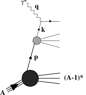
Fig. 6.1: Impulse approximation for deep-inelastic scattering from nuclei at large $Q^{2}$.

Given the small average momenta of the weakly bound nucleons, their quark sub-structure is described by structure functions similar to those of free nucleons [190, 213]. For a nucleon with momentum $p$ these structure functions depend on the scaling variable $x=Q^{2}/2p\cdot q$ and on the squared momentum transfer $Q^{2}$. However since the energies and momenta of bound nucleons do not satisfy the energy-momentum relation of free nucleons, additional freedom arises.

This becomes immediately obvious from the following simple kinematic consideration. In the laboratory frame deep-inelastic scattering from a nucleon bound in a nucleus involves the removal energy, $-\varepsilon_{n}$, of the struck nucleon:

$$\varepsilon_{n}=M_{{\mathrm{A}}}-M^{(n)}_{{{\mathrm{A-1}}}}-M.$$ (6.1)

Here $M_{{\mathrm{A}}}$ and $M^{(n)}_{{\mathrm{A-1}}}$ denote the invariant masses of the initial nuclear ground state and of the nuclear system, with a nucleon-hole state characterized by its quantum numbers $n$. The energy of the interacting nucleon is then:

$$p_{0}=M+\varepsilon_{n}-T_{{\mathrm{R}}},$$ (6.2)

where $T_{{\mathrm{R}}}={\mathchoice{\mbox{\boldmath$p$}}{\mbox{\boldmath$p$}}{\kern-0.20004pt\hbox{$\scriptstyle p$}\kern-3.52188pt\kern 0.39993pt\hbox{$\scriptstyle p$}\kern-3.52188pt\kern-0.20004pt\raise 0.21698pt\hbox{$\scriptstyle p$}}{\kern-0.20004pt\hbox{$\scriptscriptstyle p$}\kern-2.51563pt\kern 0.39993pt\hbox{$\scriptscriptstyle p$}\kern-2.51563pt\kern-0.20004pt\raise 0.21698pt\hbox{$\scriptscriptstyle p$}}^{2}}/{2M^{(n)}_{{\mathrm{A-1}}}}$ is the recoil energy of the residual nuclear system. We finally obtain for the squared four-momentum of this interacting nucleon:

$$p^{2}=p_{0}^{2}-\mathchoice{\mbox{\boldmath$p$}}{\mbox{\boldmath$p$}}{\kern-0.20004pt\hbox{$\scriptstyle p$}\kern-3.52188pt\kern 0.39993pt\hbox{$\scriptstyle p$}\kern-3.52188pt\kern-0.20004pt\raise 0.21698pt\hbox{$\scriptstyle p$}}{\kern-0.20004pt\hbox{$\scriptscriptstyle p$}\kern-2.51563pt\kern 0.39993pt\hbox{$\scriptscriptstyle p$}\kern-2.51563pt\kern-0.20004pt\raise 0.21698pt\hbox{$\scriptscriptstyle p$}}^{2}\simeq M^{2}+2M(\varepsilon_{n}-T_{{\mathrm{R}}}-T)\neq M^{2},$$ (6.3)

with $T=\mathchoice{\mbox{\boldmath$p$}}{\mbox{\boldmath$p$}}{\kern-0.20004pt\hbox{$\scriptstyle p$}\kern-3.52188pt\kern 0.39993pt\hbox{$\scriptstyle p$}\kern-3.52188pt\kern-0.20004pt\raise 0.21698pt\hbox{$\scriptstyle p$}}{\kern-0.20004pt\hbox{$\scriptscriptstyle p$}\kern-2.51563pt\kern 0.39993pt\hbox{$\scriptscriptstyle p$}\kern-2.51563pt\kern-0.20004pt\raise 0.21698pt\hbox{$\scriptscriptstyle p$}}^{2}/2M$. The squared four-momentum of the active nucleon is obviously not restricted by its free invariant mass. It is determined by the nuclear wave function which describes the momentum distributions of bound target nucleons as well as the mass spectrum of the residual nuclear system. Consequently, the structure function of a bound nucleon can in general depend also on $p^{2}$, not just on $x$ and $Q^{2}$.

6.2 Corrections from binding and Fermi motion

In the impulse approximation deep-inelastic scattering from a nucleus at large $Q^{2}$ proceeds in two steps as shown in Fig.6.1: the exchanged virtual photon scatters from a quark with momentum $k$. This quark belongs to a nucleon with momentum $p$ which is removed from the target nucleus. Treating the nucleus as a non-relativistic bound state, the nuclear structure functions factorize into two terms [190]: the information about the quark and gluon substructure of the nucleons is included in the bound nucleon structure functions $F_{1}^{{\mathrm{N}}}(x/y,p^{2})$ and $F_{2}^{{\mathrm{N}}}(x/y,p^{2})$. They depend on the fraction $x/y=k\cdot q/p\cdot q\approx k^{+}/p^{+}$ of the light-cone momentum of the interacting nucleon carried by the quark, and reduce to the corresponding free nucleon structure functions at $p^{2}=M^{2}$. Details about nuclear structure are incorporated in the distribution function of nucleons with squared four-momentum $p^{2}$ and a fraction $y$ of the nuclear light-cone momentum:

$$D_{\rm N/A}(y,p^{2}) = \intop\!\frac{d^{4}p^{\prime}}{(2\pi)^{4}}\,{\cal S}(p^{\prime})\left(1+\frac{p^{\prime}_{3}}{M}\right)\delta\left(y-\frac{p^{\prime+}}{M}\right)\,\delta(p^{2}-{p^{\prime}}^{2}).$$ (6.4)

Here

$${\cal S}(p)=2\pi\sum_{n}\delta(p_{0}-M-\varepsilon_{n}+T_{{\mathrm{R}}})\left|\mathchar 9\relax_{n}({\mathchoice{\mbox{\boldmath$p$}}{\mbox{\boldmath$p$}}{\kern-0.20004pt\hbox{$\scriptstyle p$}\kern-3.52188pt\kern 0.39993pt\hbox{$\scriptstyle p$}\kern-3.52188pt\kern-0.20004pt\raise 0.21698pt\hbox{$\scriptstyle p$}}{\kern-0.20004pt\hbox{$\scriptscriptstyle p$}\kern-2.51563pt\kern 0.39993pt\hbox{$\scriptscriptstyle p$}\kern-2.51563pt\kern-0.20004pt\raise 0.21698pt\hbox{$\scriptscriptstyle p$}}})\right|^{2}$$ (6.5)

is the spectral function of a nucleon in the nucleus. It is determined by the momentum space amplitude $\mathchar 9\relax_{n}({\mathchoice{\mbox{\boldmath$p$}}{\mbox{\boldmath$p$}}{\kern-0.20004pt\hbox{$\scriptstyle p$}\kern-3.52188pt\kern 0.39993pt\hbox{$\scriptstyle p$}\kern-3.52188pt\kern-0.20004pt\raise 0.21698pt\hbox{$\scriptstyle p$}}{\kern-0.20004pt\hbox{$\scriptscriptstyle p$}\kern-2.51563pt\kern 0.39993pt\hbox{$\scriptscriptstyle p$}\kern-2.51563pt\kern-0.20004pt\raise 0.21698pt\hbox{$\scriptscriptstyle p$}}})=\langle({{\mathrm{A-1}}})_{n},-{\mathchoice{\mbox{\boldmath$p$}}{\mbox{\boldmath$p$}}{\kern-0.20004pt\hbox{$\scriptstyle p$}\kern-3.52188pt\kern 0.39993pt\hbox{$\scriptstyle p$}\kern-3.52188pt\kern-0.20004pt\raise 0.21698pt\hbox{$\scriptstyle p$}}{\kern-0.20004pt\hbox{$\scriptscriptstyle p$}\kern-2.51563pt\kern 0.39993pt\hbox{$\scriptscriptstyle p$}\kern-2.51563pt\kern-0.20004pt\raise 0.21698pt\hbox{$\scriptscriptstyle p$}}}|\hat{\mathchar 9\relax}(0)|{{\mathrm{A}}}\rangle$, with $\hat{\mathchar 9\relax}(0)$ representing the non-relativistic nucleon field operator at the origin ${\mathchoice{\mbox{\boldmath$r$}}{\mbox{\boldmath$r$}}{\kern-0.20004pt\hbox{$\scriptstyle r$}\kern-3.35255pt\kern 0.39993pt\hbox{$\scriptstyle r$}\kern-3.35255pt\kern-0.20004pt\raise 0.21698pt\hbox{$\scriptstyle r$}}{\kern-0.20004pt\hbox{$\scriptscriptstyle r$}\kern-2.39467pt\kern 0.39993pt\hbox{$\scriptscriptstyle r$}\kern-2.39467pt\kern-0.20004pt\raise 0.21698pt\hbox{$\scriptscriptstyle r$}}}=0$. The squared amplitude $|\mathchar 9\relax_{n}({\mathchoice{\mbox{\boldmath$p$}}{\mbox{\boldmath$p$}}{\kern-0.20004pt\hbox{$\scriptstyle p$}\kern-3.52188pt\kern 0.39993pt\hbox{$\scriptstyle p$}\kern-3.52188pt\kern-0.20004pt\raise 0.21698pt\hbox{$\scriptstyle p$}}{\kern-0.20004pt\hbox{$\scriptscriptstyle p$}\kern-2.51563pt\kern 0.39993pt\hbox{$\scriptscriptstyle p$}\kern-2.51563pt\kern-0.20004pt\raise 0.21698pt\hbox{$\scriptscriptstyle p$}}})|^{2}$ describes the probability of finding a nucleon with momentum $p$ in the nuclear ground state $|{{\mathrm{A}}}\rangle$, and the remaining ${A}-1$ nucleons in a state $n$ with total momentum $-\mathchoice{\mbox{\boldmath$p$}}{\mbox{\boldmath$p$}}{\kern-0.20004pt\hbox{$\scriptstyle p$}\kern-3.52188pt\kern 0.39993pt\hbox{$\scriptstyle p$}\kern-3.52188pt\kern-0.20004pt\raise 0.21698pt\hbox{$\scriptstyle p$}}{\kern-0.20004pt\hbox{$\scriptscriptstyle p$}\kern-2.51563pt\kern 0.39993pt\hbox{$\scriptscriptstyle p$}\kern-2.51563pt\kern-0.20004pt\raise 0.21698pt\hbox{$\scriptscriptstyle p$}}$. In Eq.(6.5) the sum over a complete set of states with ${A-1}$ nucleons is taken. Note that the spectral function is normalized to $A$, the total number of nucleons in the nucleus. This leads to the proper normalization of the nucleon distribution function in Eq.(6.4) (see e.g. Refs.[2, 214, 215]).

The nuclear structure functions are then obtained by a convolution over the squared four-momentum of the interacting nucleons and their light-cone momentum fraction. For the structure function $F_{2}^{{\mathrm{A}}}$ per nucleon this gives [190]:

$$A\,F_{2}^{{\mathrm{A}}}(x)=\intop\limits_{x}^{A}\!dy\intop\!dp^{2}\,D_{\rm N/A}(y,p^{2})F_{2}^{{\mathrm{N}}}(x/y,p^{2}),$$ (6.6)

where we have suppressed the dependence on $Q^{2}$ for convenience.

In the following we examine the convolution integral (6.6) in more detail. The momentum distribution of nucleons in the nuclear target,

$$\intop\frac{dp_{0}}{2\pi}{\cal S}(p)=\sum_{n}\left|\mathchar 9\relax_{n}({\mathchoice{\mbox{\boldmath$p$}}{\mbox{\boldmath$p$}}{\kern-0.20004pt\hbox{$\scriptstyle p$}\kern-3.52188pt\kern 0.39993pt\hbox{$\scriptstyle p$}\kern-3.52188pt\kern-0.20004pt\raise 0.21698pt\hbox{$\scriptstyle p$}}{\kern-0.20004pt\hbox{$\scriptscriptstyle p$}\kern-2.51563pt\kern 0.39993pt\hbox{$\scriptscriptstyle p$}\kern-2.51563pt\kern-0.20004pt\raise 0.21698pt\hbox{$\scriptscriptstyle p$}}})\right|^{2},$$ (6.7)

falls rapidly with increasing $|\mathchoice{\mbox{\boldmath$p$}}{\mbox{\boldmath$p$}}{\kern-0.20004pt\hbox{$\scriptstyle p$}\kern-3.52188pt\kern 0.39993pt\hbox{$\scriptstyle p$}\kern-3.52188pt\kern-0.20004pt\raise 0.21698pt\hbox{$\scriptstyle p$}}{\kern-0.20004pt\hbox{$\scriptscriptstyle p$}\kern-2.51563pt\kern 0.39993pt\hbox{$\scriptscriptstyle p$}\kern-2.51563pt\kern-0.20004pt\raise 0.21698pt\hbox{$\scriptscriptstyle p$}}|$. This implies that the nucleon light-cone distribution (6.4) is strongly peaked around $y\approx 1$ and $p^{2}\approx M^{2}$, with a typical width $\mathchar 1\relax y\sim p_{F}/M$ controlled by the Fermi momentum $p_{F}$. Expanding the bound nucleon structure function in Eq.(6.6) in a Taylor series around $y=1$ and $p^{2}=M^{2}$, and integrating term by term, leads to the following expression for the nuclear structure function per nucleon [190, 214], valid in the range $0.2<x<0.7$:

$$F^{{\mathrm{A}}}_{2}(x)\approx F_{2}^{{\mathrm{N}}}(x)-\frac{\langle\varepsilon\rangle}{M}\>x{F_{2}^{{\mathrm{N}}}}^{\prime}(x)+\frac{\langle T\rangle}{3M}\>x^{2}{F_{2}^{{\mathrm{N}}}}^{\prime\prime}(x)$$

$$+2\>\frac{\langle\varepsilon\rangle-\langle T\rangle}{M}\left(p^{2}\frac{\partial F_{2}^{{\mathrm{N}}}(x;p^{2})}{\partial p^{2}}\right)_{p^{2}=M^{2}},$$ (6.8)

where ${F_{2}^{{\mathrm{N}}}}^{\prime}(x)$ and ${F_{2}^{{\mathrm{N}}}}^{\prime\prime}(x)$ are derivatives of the structure function with respect to $x$. The mean value of the single particle energy $\varepsilon=p_{0}-M$ is

$$\langle\varepsilon\rangle = {1\over{{\mathrm{A}}}}\intop\!\frac{d^{4}p}{(2\pi)^{4}}\,{\cal S}(p)\,\varepsilon,$$ (6.9)

and

$$\langle T\rangle = {1\over{{\mathrm{A}}}}\intop\!\frac{d^{4}p}{(2\pi)^{4}}\,{\cal S}(p)\,\frac{{\mathchoice{\mbox{\boldmath$p$}}{\mbox{\boldmath$p$}}{\kern-0.20004pt\hbox{$\scriptstyle p$}\kern-3.52188pt\kern 0.39993pt\hbox{$\scriptstyle p$}\kern-3.52188pt\kern-0.20004pt\raise 0.21698pt\hbox{$\scriptstyle p$}}{\kern-0.20004pt\hbox{$\scriptscriptstyle p$}\kern-2.51563pt\kern 0.39993pt\hbox{$\scriptscriptstyle p$}\kern-2.51563pt\kern-0.20004pt\raise 0.21698pt\hbox{$\scriptscriptstyle p$}}}^{2}}{2M}$$ (6.10)

represents the mean kinetic energy of bound nucleons. Except for light nuclei the recoil energy $T_{{\mathrm{R}}}$ in Eq.(6.2) can be neglected. Then $\langle\varepsilon\rangle$ coincides with the separation energy. Corrections to Eq.(6.2) are of higher order in $\langle\varepsilon\rangle/M$ and $\langle T\rangle/M$. Note that the approximate result for $F_{2}^{{\mathrm{A}}}$ in Eq.(6.2) is well justified in the region $0.2<x<0.7$. Here the kinematic condition $x/y<1$ in Eq.(6.6) can be ignored in accordance with the underlying expansion.

Let us briefly discuss the physical meaning of the different terms in Eq.(6.2) and their implications. The second term on the right hand side of Eq.(6.2) involves the average separation energy of nucleons from the target. As such it is determined by nuclear binding. In the range $0.2<x<0.7$ it leads to a depletion of the nuclear structure function compared to the structure function of a free nucleon. The third term accounts for the Fermi motion of bound nucleons and yields a strong rise of the structure function ratio $F_{2}^{{\mathrm{A}}}/F_{2}^{{\mathrm{N}}}$ at large $x$. Finally, the fourth term in (6.2) reflects the dependence of the structure function of a bound nucleon on its squared four-momentum. Note that this contribution enters at the same order as binding and Fermi-motion corrections. Information about the $p^{2}$-dependence of bound nucleon structure functions is rare. Nevertheless such effects may lead to significant modifications of the EMC ratio $F_{2}^{{\mathrm{A}}}/F_{2}^{{\mathrm{N}}}$ at moderate and large values of $x$. This has been shown for example in the framework of a simple quark-diquark picture for the nucleon [190].

An important and not yet completely solved problem with respect to the binding and Fermi-motion corrections in Eq.(6.2) is a reliable calculation of $\langle\varepsilon\rangle$ and $\langle T\rangle$. In a simple nuclear shell model the separation energy is averaged over all occupied levels. One finds typical values $\langle\varepsilon\rangle\approx-(20-25)\;$MeV and $\langle T\rangle\approx 18-20\;$MeV. Correlations between nucleons change the simple mean field picture substantially and lead to high momentum components with $|\mathchoice{\mbox{\boldmath$p$}}{\mbox{\boldmath$p$}}{\kern-0.20004pt\hbox{$\scriptstyle p$}\kern-3.52188pt\kern 0.39993pt\hbox{$\scriptstyle p$}\kern-3.52188pt\kern-0.20004pt\raise 0.21698pt\hbox{$\scriptstyle p$}}{\kern-0.20004pt\hbox{$\scriptscriptstyle p$}\kern-2.51563pt\kern 0.39993pt\hbox{$\scriptscriptstyle p$}\kern-2.51563pt\kern-0.20004pt\raise 0.21698pt\hbox{$\scriptscriptstyle p$}}|>p_{F}$ in the nuclear spectral function (6.5). This in turn causes an increase of the average separation energy $\langle\varepsilon\rangle$ [216, 217]. In order to see this let us examine the Koltun sum rule [218]

$$\langle\varepsilon\rangle+\langle T\rangle=-2\mu_{B},$$ (6.11)

where $\mu_{B}$ is the binding energy per nucleon. This sum rule is exact if only two-body forces are present in the nuclear Hamiltonian. With fixed $\mu_{B}\approx 8\,$MeV, this sum rule tells that an increase of $\langle T\rangle$ due to high momentum components is accompanied by an increase of $|\langle\varepsilon\rangle|$. We refer in this context to a calculation [219] of the spectral function of nuclear matter based on a variational method. This calculation shows that there is a significant probability to find nucleons with high momentum and large separation energies. An integration of the spectral function of Ref.[219] gives $\langle T\rangle\approx 38\;$MeV and $\langle\varepsilon\rangle\approx-70\;$MeV [217]. In order to estimate these quantities for heavy nuclei one usually assumes [216] that the high momentum components of the nucleon momentum distribution are about the same as in nuclear matter. Together with Eq.(6.11) this leads to $\langle\varepsilon\rangle\approx-50\;$MeV.

In Fig.6.2 we show typical results from Refs.[190, 215] for iron and gold. We observe that a qualitative understanding of the EMC effect can indeed be reached, but at $x\mathrel{\raise 2.58334pt\hbox{$>$}\kern-7.7778pt\lower 2.79857pt\hbox{$\sim$}}0.5$ a more quantitative description is still lacking. One should note, of course, that the presentation of nuclear effects in terms of the ratio $F_{2}^{{\mathrm{A}}}/F_{2}^{{\mathrm{N}}}$ magnifies such effects in a misleading manner because $F_{2}^{{\mathrm{N}}}$ itself is small in this region (see also the discussion in Section 4.4).

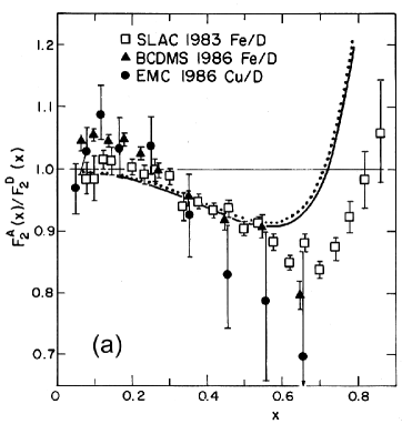
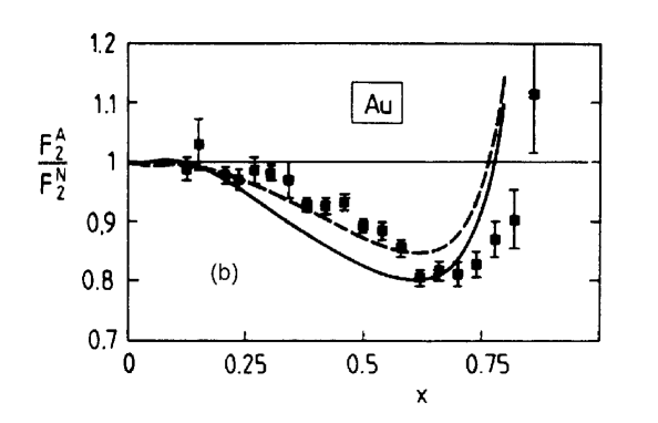
Fig. 6.2: The ratio of nuclear and nucleon structure functions, $F_{2}^{{\mathrm{A}}}/F_{2}^{N}$, for iron and gold taken from Refs.[215, 190]. (a) solid curve: calculation in Ref.[215], dotted curve: calculation in Ref.[214]. (b) results from Ref.[190]: without $p^{2}$-dependence of the bound nucleon structure function (dashed), and including this $p^{2}$-dependence as obtained from a simple quark-diquark picture (full).

The impulse approximation picture of nuclear deep-inelastic scattering can also be maintained in a relativistically covariant way [212]. Here, however, a simple factorization of nuclear structure functions into nuclear and nucleon parts as in Eq.(6.6) is not possible any longer. A relativistic calculation of nuclear structure functions requires relativistic nuclear wave functions as well as a more detailed knowledge about the structure of bound nucleons. Nevertheless, relativistic effects seem to be small: in an explicit model calculation of the deuteron structure function $F_{2}^{{\mathrm{d}}}$ relativistic corrections to the non-relativistic convolution (6.6) are less than $2\%$ for $x<0.9$ [220]. In the region $x>1$, where nuclear structure functions are very small however, larger deviations are expected.

In this context a word of caution is in order. A description of nuclear structure functions based on nucleons alone is necessarily incomplete since it violates the momentum sum rule [1]. Non-nucleonic degrees of freedom are briefly discussed in Section 6.5.

6.3 Beyond the impulse approximation

The quality of the impulse approximation has frequently been questioned (see e.g. Refs.[1, 5, 190, 210, 211, 212] and references therein). Here we give a brief summary of possible shortcomings in terms of models for nuclear deep-inelastic scattering which go beyond this approximation.

6.3.1 Quark exchange in nuclei

The impulse approximation includes only incoherent scattering processes from hadronic constituents of the target nucleus. On the other hand, contributions involving several bound nucleons could also be important, and their role needs to be examined.

One such possibility, namely quark exchange between different nucleons, has been investigated in Refs.[210, 221]. The nuclear quark wave function which is probed in deep-inelastic scattering must be antisymmetric with respect to permutations of quarks. This however is not realized in the impulse approximation (6.6). Antisymmetrization introduces additional quark exchange terms between different nucleons in the target.

Under several simplifying assumptions a softening of the nuclear quark momentum distribution due to quark exchange has been found. For small nuclei the effect turned out to be significant. For ${}^{4}\rm{He}$ approximately $30\%$ of the observed depletion of the structure function ratio $F_{2}^{{\mathrm{He}}}/F_{2}^{{\mathrm{N}}}$ at $x\sim 0.6$ has been associated with quark exchange. Only minor modifications have been found for heavier nuclei [221].

While the estimates based on a simple quark exchange model may not be reliable at a quantitative level, they certainly point to the fact that the impulse approximation is incomplete as soon as correlations between quarks in several nucleons come into play.

6.3.2 Final state interactions in a mean field approach

One of the basic assumptions of the impulse approximation is that interactions of the struck, highly excited nucleon with the residual nuclear system can be ignored. In general there is no solid basis for this assumption since the debris of the struck nucleon includes also low momentum fragments as seen from the target rest frame. A proper treatment of their final state interaction requires however a description of the nucleus in terms of quark and gluon degrees of freedom.

Investigations in this direction have been made starting out from a quark model for nuclear matter, with nucleons modeled as non-overlapping MIT bags [211, 222, 223]. The nucleons interact via the exchange of scalar and vector mesons which couple directly to quarks. Within the mean field approximation for the meson fields it is possible to describe several basic properties of nuclear matter, such as its compressibility and the binding energy per nucleon at saturation density.

This model has been applied to deep-inelastic scattering from finite nuclei using a local density approximation [211]. The debris of the struck nucleon is represented by a pair of spectator quarks bound in a diquark bag. Its interaction with the remaining nuclear system in the final state leads to a non-negligible effect on nuclear structure functions: while the full calculation including final state interactions allows to reproduce the structure function ratio $F_{2}^{A}/F_{2}^{N}$, the impulse approximation overestimates nuclear effects at $x\sim 0.6$ by about a factor two. In the framework of this model such a difference is expected since the binding of the nucleus is the result of the attractive scalar mean field experienced by all three constituent quarks of the interacting nucleon. When ignoring the binding of the spectator quark pair, as done in the impulse approximation, one assumes that the active quark which takes part in the deep-inelastic scattering process behaves as if it carries the binding of all three quarks, a feature which obviously needs to be corrected.

The mean field approach to nuclear quark distributions is based on several simplifying assumptions, but it nevertheless points to the possible importance of final state interactions and, in more general terms, to the relevance of quark degrees of freedom in nuclei.

6.4 Modifications of bound nucleon structure functions

The intrinsic properties of nucleons bound in nuclei can be modified as compared to free nucleons. We summarize below two examples of models which deal with such possible changes in bound nucleon structure functions.

6.4.1 Rescaling

At intermediate values of the Bjorken variable, $0.2<x<0.7$, the modification of nuclear structure functions $F_{2}^{{\mathrm{A}}}$ as compared to the free nucleon structure function $F_{2}^{{\mathrm{N}}}$ can be described by a shift in the momentum scale which enters the structure functions. We briefly outline here the basic arguments [224, 225, 226, 227, 228]. Consider the moments

$$M_{n}^{{\mathrm{A}}}(Q^{2})=\intop_{0}^{A}dx\,x^{n-2}F_{2}^{{{\mathrm{A}}}}(x,Q^{2}),\quad{\rm with}\;n\;{\rm{even}}.$$ (6.12)

Assume now that the moments of nuclear and nucleon structure functions are related by a shift of their momentum scale:

$$M_{n}^{{\mathrm{A}}}(\mu_{{\mathrm{A}}}^{2})=M_{n}^{{\mathrm{N}}}(\mu_{{\mathrm{N}}}^{2}).$$ (6.13)

At an arbitrary momentum transfer $Q^{2}$ the perturbative QCD evolution equations to leading order (see Section 2.4) give:

$$M_{n}^{{\mathrm{A}}}(Q^{2})=M_{n}^{{\mathrm{N}}}\left(\xi_{{\mathrm{A}}}(Q^{2})Q^{2}\right),$$ (6.14)

with the rescaling parameter

$$\xi_{{\mathrm{A}}}(Q^{2})=\left(\frac{\mu_{{\mathrm{N}}}^{2}}{\mu_{{\mathrm{A}}}^{2}}\right)^{\frac{\alpha_{s}(\mu_{{\mathrm{A}}}^{2})}{\alpha_{s}(Q^{2})}}.$$ (6.15)

Of course Eq.(6.14) can always be satisfied if one allows different $\xi_{{\mathrm{A}}}$ for different moments $n$. However, when comparing with data it has turned out that the rescaling parameter is independent of $n$ to a good approximation. Consequently, the scale change for the moments (6.14) can be translated directly into a scale change for the structure functions themselves:

$$F_{2}^{{\mathrm{A}}}(x,Q^{2})=F_{2}^{{\mathrm{N}}}\left(x,\xi_{{\mathrm{A}}}(Q^{2})Q^{2}\right).$$ (6.16)

Good agreement with experimental data can be achieved at intermediate $x$. For example, the EMC structure function data on iron suggest $\xi_{\rm Fe}\approx 2$ for $Q^{2}=20$ GeV² [226].

Rescaling gives a reasonable one-parameter description of nuclear structure functions $F_{2}^{{\mathrm{A}}}$ at intermediate $x$, but it does not offer insights into the physical origin of the observed change of scale. One possible suggestion to explain the scale change is a modification of the effective confinement scale for quarks in the nucleus as compared to free nucleons [224, 225, 226].

Scale changes are not simply related to possible “swelling” of nucleons inside nuclei which is constrained by inclusive electron-nucleus scattering data in the quasielastic region. The experimentally observed $y$-scaling indicates a rather small increase of the charge radius for bound nucleons. For example, the study of [229, 230] comes to the conclusion that any increase of the nuclear radius in nuclei should be less than $6\%$ of its free radius.

Related discussions and a comparison with nuclear DIS data can be found in Refs.[202,216,231–234].

6.4.2 Color screening in bound nucleons

The scenario of Refs.[1, 235, 236] assumes that the dominant contribution to the structure function $F_{2}^{{\mathrm{N}}}$ at large $x\sim 0.6$ is given by small size (pointlike) parton configurations in the nucleon. In a nuclear environment such configurations interact only weakly with other nucleons due to the screening of their color charge. It is argued that the probability for pointlike configurations is reduced in bound nucleons. In fact, the probability to find parton configurations of average size in the nucleon should actually be enhanced in nuclei since they experience the attraction of the nuclear mean field. Then the variational principle with normalization condition on the wave function implies that small-size configurations should indeed be suppressed.

An estimate of such deformations in the wave function of nucleons bound in heavy nuclei gives for $x\sim 0.5$ [235]:

$$\frac{F_{2}^{{\mathrm{A}}}}{F_{2}^{{\mathrm{N}}}}\sim 1+\frac{4\,\langle U\rangle}{E^{*}}\sim 0.7\,\mbox{--}\,0.8.$$ (6.17)

Here $\langle U\rangle$ is the average potential energy per nucleon, $\langle U\rangle\sim-40$ MeV, and $E^{*}\sim 0.5$ GeV is the typical energy scale for excitations of the nucleon. Since $\langle U\rangle$ scales with the nuclear density, the nuclear dependence of the structure function ratio (6.17) is roughly consistent with data.

It should be mentioned that the proposed suppression of rather rare pointlike configurations in bound nucleons does not necessarily imply a substantial change of average properties of a bound nucleon, such as its electromagnetic radius [1].

6.5 Pion contributions to nuclear structure functions

In conventional nuclear physics meson exchange is responsible for the binding of nucleons in the nucleus. Therefore deep-inelastic scattering from mesons present in the nuclear wave function should give additional contributions to nuclear structure functions. Pions, which are responsible for most of the intermediate- and long-range nucleon-nucleon force, are supposed to play the prominent role (see e.g. [237, 238, 239, 240, 241]).

The framework is the Sullivan process [242]. Its contribution to the nucleon structure function $F_{2}^{{\mathrm{N}}}$ reads:

$$\delta^{\pi}F_{2}^{{\mathrm{N}}}(x)=\intop_{x}^{1}{{\mathrm{d}}}y\,f_{{{\mathrm{\pi/N}}}}(y)\,F_{2}^{{{\mathrm{\pi}}}}(x/y),$$ (6.18)

where

$$f_{{\mathrm{\pi/N}}}(y)=\frac{3g^{2}_{{\mathrm{\pi NN}}}}{16\pi^{2}}\intop^{t_{min}}_{-\infty}{{\mathrm{d}}}t\frac{-t|{\cal F}_{{{\mathrm{\pi NN}}}}(t)|^{2}}{(t-m_{{{\mathrm{\pi}}}}^{2})^{2}}\,y$$ (6.19)

specifies the distribution of pions with light-cone momentum fraction $y$ in the nucleon, while $F_{2}^{{{\mathrm{\pi}}}}$ is the pion structure function. Equation (6.18) describes deep-inelastic scattering from a pion emitted from its nucleon source. The nucleon receives a momentum transfer equal to the pion momentum $k^{\mu}=(\omega,\mathchoice{\mbox{\boldmath$k$}}{\mbox{\boldmath$k$}}{\kern-0.20004pt\hbox{$\scriptstyle k$}\kern-3.86458pt\kern 0.39993pt\hbox{$\scriptstyle k$}\kern-3.86458pt\kern-0.20004pt\raise 0.21698pt\hbox{$\scriptstyle k$}}{\kern-0.20004pt\hbox{$\scriptscriptstyle k$}\kern-2.7604pt\kern 0.39993pt\hbox{$\scriptscriptstyle k$}\kern-2.7604pt\kern-0.20004pt\raise 0.21698pt\hbox{$\scriptscriptstyle k$}})$. The minimal squared momentum transfer $t=k^{2}$ required for pion emission is $t_{min}=-M^{2}y^{2}/(1-y)$. One finds that $\delta^{{\mathrm{\pi}}}F_{2}^{{\mathrm{N}}}$ gets its dominant contributions from pions with momenta $|\mathchoice{\mbox{\boldmath$k$}}{\mbox{\boldmath$k$}}{\kern-0.20004pt\hbox{$\scriptstyle k$}\kern-3.86458pt\kern 0.39993pt\hbox{$\scriptstyle k$}\kern-3.86458pt\kern-0.20004pt\raise 0.21698pt\hbox{$\scriptstyle k$}}{\kern-0.20004pt\hbox{$\scriptscriptstyle k$}\kern-2.7604pt\kern 0.39993pt\hbox{$\scriptscriptstyle k$}\kern-2.7604pt\kern-0.20004pt\raise 0.21698pt\hbox{$\scriptscriptstyle k$}}|\simeq 300-400$ MeV. Pions with smaller momenta are suppressed by the explicit factor $y$ in Eq.(6.19), while pions with large momenta are suppressed by the pion propagator and the ${\mathrm{\pi NN}}$ form factor ${\cal F}_{{\mathrm{\pi NN}}}$ [237].

The convolution ansatz in Eq.(6.18) suffers from similar problems as convolution for nuclear structure functions discussed in Section 6.2: the interacting pion is not on its mass shell, i.e. $k^{2}\approx-\mathchoice{\mbox{\boldmath$k$}}{\mbox{\boldmath$k$}}{\kern-0.20004pt\hbox{$\scriptstyle k$}\kern-3.86458pt\kern 0.39993pt\hbox{$\scriptstyle k$}\kern-3.86458pt\kern-0.20004pt\raise 0.21698pt\hbox{$\scriptstyle k$}}{\kern-0.20004pt\hbox{$\scriptscriptstyle k$}\kern-2.7604pt\kern 0.39993pt\hbox{$\scriptscriptstyle k$}\kern-2.7604pt\kern-0.20004pt\raise 0.21698pt\hbox{$\scriptscriptstyle k$}}^{2}\neq m_{\pi}^{2}$. Therefore the pion structure function depends also on $k^{2}$. Furthermore, final state interactions of the pion debris with the recoil nucleon are neglected.

The detailed treatment of pionic effects in nuclei includes the pion propagation in the medium with $\mathchar 1\relax$ resonance excitation, Pauli effects and short range spin-isospin correlations. All these effects are incorporated in the pion-nuclear response function $R(\mathchoice{\mbox{\boldmath$k$}}{\mbox{\boldmath$k$}}{\kern-0.20004pt\hbox{$\scriptstyle k$}\kern-3.86458pt\kern 0.39993pt\hbox{$\scriptstyle k$}\kern-3.86458pt\kern-0.20004pt\raise 0.21698pt\hbox{$\scriptstyle k$}}{\kern-0.20004pt\hbox{$\scriptscriptstyle k$}\kern-2.7604pt\kern 0.39993pt\hbox{$\scriptscriptstyle k$}\kern-2.7604pt\kern-0.20004pt\raise 0.21698pt\hbox{$\scriptscriptstyle k$}},\omega)$ which determines the spectrum of pionic excitations in the nuclear medium. The resulting distribution function of pions in a nucleus is [237]

$$f_{{\mathrm{\pi}}/{{\mathrm{A}}}}(y)=\frac{3g^{2}_{{\mathrm{\pi NN}}}}{16\pi^{2}}y\intop_{M^{2}y^{2}}^{\infty}{{\mathrm{d}}}|\mathchoice{\mbox{\boldmath$k$}}{\mbox{\boldmath$k$}}{\kern-0.20004pt\hbox{$\scriptstyle k$}\kern-3.86458pt\kern 0.39993pt\hbox{$\scriptstyle k$}\kern-3.86458pt\kern-0.20004pt\raise 0.21698pt\hbox{$\scriptstyle k$}}{\kern-0.20004pt\hbox{$\scriptscriptstyle k$}\kern-2.7604pt\kern 0.39993pt\hbox{$\scriptscriptstyle k$}\kern-2.7604pt\kern-0.20004pt\raise 0.21698pt\hbox{$\scriptscriptstyle k$}}|^{2}\intop_{0}^{|\mathchoice{\mbox{\boldmath$k$}}{\mbox{\boldmath$k$}}{\kern-0.14003pt\hbox{$\scriptstyle k$}\kern-2.7052pt\kern 0.27995pt\hbox{$\scriptstyle k$}\kern-2.7052pt\kern-0.14003pt\raise 0.15189pt\hbox{$\scriptstyle k$}}{\kern-0.14003pt\hbox{$\scriptscriptstyle k$}\kern-1.93228pt\kern 0.27995pt\hbox{$\scriptscriptstyle k$}\kern-1.93228pt\kern-0.14003pt\raise 0.15189pt\hbox{$\scriptscriptstyle k$}}|-My}{{\mathrm{d}}}\omega\,\frac{\mathchoice{\mbox{\boldmath$k$}}{\mbox{\boldmath$k$}}{\kern-0.20004pt\hbox{$\scriptstyle k$}\kern-3.86458pt\kern 0.39993pt\hbox{$\scriptstyle k$}\kern-3.86458pt\kern-0.20004pt\raise 0.21698pt\hbox{$\scriptstyle k$}}{\kern-0.20004pt\hbox{$\scriptscriptstyle k$}\kern-2.7604pt\kern 0.39993pt\hbox{$\scriptscriptstyle k$}\kern-2.7604pt\kern-0.20004pt\raise 0.21698pt\hbox{$\scriptscriptstyle k$}}^{2}|{\cal F}_{{{\mathrm{\pi NN}}}}(\mathchoice{\mbox{\boldmath$k$}}{\mbox{\boldmath$k$}}{\kern-0.20004pt\hbox{$\scriptstyle k$}\kern-3.86458pt\kern 0.39993pt\hbox{$\scriptstyle k$}\kern-3.86458pt\kern-0.20004pt\raise 0.21698pt\hbox{$\scriptstyle k$}}{\kern-0.20004pt\hbox{$\scriptscriptstyle k$}\kern-2.7604pt\kern 0.39993pt\hbox{$\scriptscriptstyle k$}\kern-2.7604pt\kern-0.20004pt\raise 0.21698pt\hbox{$\scriptscriptstyle k$}}^{2})|^{2}}{(t-m_{{{\mathrm{\pi}}}}^{2})^{2}}\,R(|\mathchoice{\mbox{\boldmath$k$}}{\mbox{\boldmath$k$}}{\kern-0.20004pt\hbox{$\scriptstyle k$}\kern-3.86458pt\kern 0.39993pt\hbox{$\scriptstyle k$}\kern-3.86458pt\kern-0.20004pt\raise 0.21698pt\hbox{$\scriptstyle k$}}{\kern-0.20004pt\hbox{$\scriptscriptstyle k$}\kern-2.7604pt\kern 0.39993pt\hbox{$\scriptscriptstyle k$}\kern-2.7604pt\kern-0.20004pt\raise 0.21698pt\hbox{$\scriptscriptstyle k$}}|,\omega),$$ (6.20)

where $t=\omega^{2}-\mathchoice{\mbox{\boldmath$k$}}{\mbox{\boldmath$k$}}{\kern-0.20004pt\hbox{$\scriptstyle k$}\kern-3.86458pt\kern 0.39993pt\hbox{$\scriptstyle k$}\kern-3.86458pt\kern-0.20004pt\raise 0.21698pt\hbox{$\scriptstyle k$}}{\kern-0.20004pt\hbox{$\scriptscriptstyle k$}\kern-2.7604pt\kern 0.39993pt\hbox{$\scriptscriptstyle k$}\kern-2.7604pt\kern-0.20004pt\raise 0.21698pt\hbox{$\scriptscriptstyle k$}}^{2}$. Using the the Sullivan description (6.18) the contribution of excess pions to the nuclear structure function $F_{2}^{{\mathrm{A}}}$ can be calculated according to:

$$\delta^{\pi}F_{2}^{{{\mathrm{A}}}}(x)=\intop_{x}^{1}{{\mathrm{d}}}y\left(f_{{{\mathrm{\pi/A}}}}(y)-f_{{{\mathrm{\pi/N}}}}(y)\right)F_{2}^{{{\mathrm{\pi}}}}(x/y).$$ (6.21)

In the original work in Ref.[237], using the empirical pion structure function, a significant enhancement of the ratio $F_{2}^{{\mathrm{A}}}/F_{2}^{{\mathrm{N}}}$ was found at $x<0.3$. This observation was in agreement with the early EMC data [74]. Later data on nuclear structure functions showed only a minor enhancement around $x\simeq 0.15$ (see Section 3.3.1). In addition Drell-Yan data from E772 [107] have demonstrated that the antiquark distribution in nuclei is not significantly enhanced as compared to free nucleons, in disagreement with the first pion model calculations. However, as already emphasized in Ref.[237], the pion contribution to nuclear structure functions is very sensitive to the strength of repulsive short range spin-isospin correlations in nuclei. Variations of this strength by $15\%$ can easily lead to $30\%$ changes in $\delta^{{\mathrm{\pi}}}F_{2}^{{\mathrm{A}}}$. While it is not difficult to accommodate the very small observed pionic enhancement within such uncertainties, it is still a challange to arrive at a consistant overall picture of nuclear DIS which rigorously satisfies the requirements of the momentum sum rule.

6.6 Further notes

Related studies of pion field effects as well as other nuclear medium corrections and their implications on nuclear DIS have been performed in Refs.[243, 244, 245, 246]. These studies include calculations within the delta-hole model [245], the role of NN correlations and the energy dependence of nuclear response functions [246], possible effects of “Brown-Rho scaling” on nuclear structure functions [243], and implications of low-energy pion-nucleus scattering data for nuclear deep-inelastic scattering and Drell-Yan production [244].

Some further investigations use a relativistic many-body approach to treat mesonic and binding corrections to reproduce nuclear effects in the EMC and Drell-Yan measurements [247, 248]. From the point of view of nuclear many-body theory, the best nuclear wave functions have been employed in Refs.[249, 250], treating both short and long range correlations in nuclear matter and helium at the most advanced level. Two-nucleon correlations turn out to be important in nuclear DIS. It should be mentioned, however, that the results of [247, 249, 250] have met with some debate concerning the proper choice of the “flux factor”. Questions of rigorous baryon number conservation [1] have also been raised.

It has been suggested to investigate intrinsic properties of bound nucleons in semi-inclusive deep-inelastic scattering from nuclei [235, 251, 252, 253]. Measuring the scattered lepton in coincidence with the residual nuclear system should provide detailed information on changes in bound nucleon structure functions. Possible experiments are discussed at HERMES [254].

7 Deep-inelastic scattering from polarized nuclei

Understanding the spin structure of the proton and the neutron is a central issue in QCD. Both the polarized neutron and proton structure functions, $g_{1}^{\rm n}$ and $g_{1}^{\rm p}$, are needed in the investigation of flavor singlet quark spin distributions (see e.g. Ref.[44]), and in the experimental test of the fundamental Bjorken sum rule (2.66).

Since free neutron targets are not available one must resort to polarized nuclei, such as the deuteron and ${}^{3}\rm{He}$, where the neutron spin plays a well defined role in building up the total polarization of the nuclear target. Polarized deep-inelastic scattering from deuterium [33, 38, 39, 43] and ${}^{3}\rm{He}$ [35, 37, 41] has been studied with high precision. In order to deduce accurate information about the individual nucleon spin structure functions from these data, it is essential to correct for genuine nuclear effects. In addition, the presence of the tensor interaction between nucleons in nuclei creates specific spin effects which are of interest in their own right.

7.1 Effective polarization

As discussed in Section 4, nuclear structure functions at Bjorken-$x>0.2$ are dominated by the incoherent scattering from bound nucleons. For polarized nuclei, the non-trivial spin-orbit structure of the wave functions causes new effects. Bound nucleons can carry orbital angular momentum, so their polarization vectors need not be aligned with the total polarization of the target nucleus: depolarization effects occur.

In order to describe such nuclear depolarization phenomena it is useful to introduce effective polarizations for nucleons bound in the nucleus. Let $|A\uparrow\rangle$ represent a nuclear state polarized in the $z$-direction. Then the effective polarization of protons or neutrons in that nucleus is

$${\cal P}_{{\mathrm{p}}}^{{\mathrm{A}}} = \left\langle A\uparrow\right|\sum_{i=protons}\sigma_{z}(i)\left|A\uparrow\right\rangle,$$ (7.1)

$${\cal P}_{{\mathrm{n}}}^{{\mathrm{A}}} = \left\langle A\uparrow\right|\sum_{i=neutrons}\sigma_{z}(i)\left|A\uparrow\right\rangle.$$ (7.2)

When the nuclear depolarization effects are described entirely in terms of these effective polarizations of bound nucleons, the nucleon spin structure functions (say, $g_{1}^{{\mathrm{A}}}$ and $g_{2}^{{\mathrm{A}}}$) have the following simple additive form:

$$g_{1,2}^{{\mathrm{A}}}(x,Q^{2})={\cal P}_{{\mathrm{p}}}^{{\mathrm{A}}}\,g_{1,2}^{{\mathrm{p}}}(x,Q^{2})+{\cal P}_{{\mathrm{n}}}^{{\mathrm{A}}}\,g_{1,2}^{{\mathrm{n}}}(x,Q^{2}).$$ (7.3)

Nuclear depolarization effects are important over the whole kinematic range of recent measurements. Within the impulse approximation these effects exceed by far the influence of nuclear binding and Fermi motion at $0.2<x<0.7$ (see Section 7.4).

7.2 Depolarization in deuterium and ³He

In case of the deuteron the effective proton and neutron polarizations are simply determined by the D-state admixture in the deuteron wave function, induced by the tensor interaction between proton and neutron in the spin triplet state. One finds:

$${\cal P}_{{\mathrm{p}}}^{{\mathrm{d}}}={\cal P}_{{\mathrm{n}}}^{{\mathrm{d}}}=1-\frac{3}{2}P_{{\mathrm{D}}}$$ (7.4)

where $P_{{\mathrm{D}}}$ is the D-state probability. The numerical values of ${\cal P}_{{\mathrm{p,n}}}^{{\mathrm{d}}}$ range between $0.91$ and $0.94$ using deuteron wave functions calculated with the Paris [152] or Bonn [195] nucleon-nucleon potential, respectively.

Apart from the interest in neutron spin structure functions the deuteron with its triplet spin structure is of interest all by itself. Its spin-$1$ property leads to additional structure functions as given in Eq.(3.3). In particular, the new spin structure functions $b_{1}$ and $b_{2}$ are accessible in deep-inelastic scattering from polarized deuterons and can be investigated in forthcoming HERMES measurements [69].

Polarized ${}^{3}{\mathrm{He}}$ can be viewed, to a first approximation, as a polarized neutron target, with the proton-neutron subsystem in a spin singlet configuration and the surplus neutron carrying the spin of the three-body system. Corrections to this picture come from the admixture of S^′- and D-wave components to the ${}^{3}{\mathrm{He}}$ wave function. The consequence is that the effective neutron polarization is reduced from unity, and the effective proton polarization does not vanish:

$${\cal P}_{{\mathrm{n}}}^{{\mathrm{He}}} = 1-\frac{2}{3}P_{{\mathrm{S}}^{\prime}}-\frac{4}{3}P_{{\mathrm{D}}}=0.86\pm 0.02,$$ (7.5)

$${\cal P}_{{\mathrm{p}}}^{{\mathrm{He}}} = -\frac{2}{3}\left(P_{{\mathrm{D}}}-P_{{\mathrm{S}}^{\prime}}\right)=-0.056\pm 0.008.$$ (7.6)

These results are obtained from three-body calculations using realistic nucleon-nucleon interactions [255], omitting however effects from meson exchange currents (see Section 7.3.4)

7.3 Nuclear coherence effects in polarized deep-inelastic scattering

Coherence phenomena such as shadowing at small Bjorken-$x$ are dominated by the interaction of diffractively excited hadronic states with several nucleons over large longitudinal distances in the target nucleus. The characteristic space-time properties of DIS are independent of the target or beam polarization. Therefore, nuclear coherence effects are also expected in polarized scattering. We explore such effects in the following for deuterium and ${}^{3}{\mathrm{He}}$.

7.3.1 Polarized single and double scattering in the deuteron

Consider the deuteron spin structure functions $g_{1}^{{\mathrm{d}}}$ and $b_{1}$ at small values of the Bjorken variable, $x<0.1$. Following the discussion in Section 3.2, these structure functions can be expressed in terms of virtual photon-deuteron helicity amplitudes. At large $Q^{2}$ in the Bjorken limit which we keep throughout this section, only the helicity conserving amplitudes enter. As usual, we choose a right-handed, transversely polarized (virtual) photon (index “$+$”) for reference. We denote the helicity conserving $\gamma^{*}{\mathrm{d}}$ amplitudes by ${\cal A}^{\gamma^{*}{\mathrm{d}}}_{+{H}}$, where ${H}=0,+,-$ refers to the helicity state of the polarized deuteron, and we choose the direction defined by the photon momentum $q$ as quantization axis. The spin structure functions of interest are then expressed as (3.7,3.9)

$$g_{1}^{\mathrm{d}} = \frac{1}{4\pi e^{2}}{\mathrm{Im}}\,\left({\cal A}^{\gamma^{*}\mathrm{d}}_{+-}-{\cal A}^{\gamma^{*}\mathrm{d}}_{++}\right),$$ (7.7)

$$b_{1} = \frac{1}{4\pi e^{2}}{\mathrm{Im}}\,\left(2{\cal A}^{\gamma^{*}\mathrm{d}}_{+0}-{\cal A}^{\gamma^{*}\mathrm{d}}_{++}-{\cal A}^{\gamma^{*}\mathrm{d}}_{+-}\right).$$ (7.8)

Let us now decompose ${\cal A}^{\gamma^{*}{\mathrm{d}}}_{+{H}}$ into incoherent, single scattering terms and a coherent double scattering contribution. We will use the non-relativistic deuteron wave function,

$$\psi_{H}(\mathchoice{\mbox{\boldmath$r$}}{\mbox{\boldmath$r$}}{\kern-0.20004pt\hbox{$\scriptstyle r$}\kern-3.35255pt\kern 0.39993pt\hbox{$\scriptstyle r$}\kern-3.35255pt\kern-0.20004pt\raise 0.21698pt\hbox{$\scriptstyle r$}}{\kern-0.20004pt\hbox{$\scriptscriptstyle r$}\kern-2.39467pt\kern 0.39993pt\hbox{$\scriptscriptstyle r$}\kern-2.39467pt\kern-0.20004pt\raise 0.21698pt\hbox{$\scriptscriptstyle r$}}) = \frac{1}{\sqrt{4\pi}}\left[\frac{u(r)}{r}+\frac{v(r)}{r}\frac{1}{\sqrt{8}}\hat{S}_{12}(\hat{\mathchoice{\mbox{\boldmath$r$}}{\mbox{\boldmath$r$}}{\kern-0.20004pt\hbox{$\scriptstyle r$}\kern-3.35255pt\kern 0.39993pt\hbox{$\scriptstyle r$}\kern-3.35255pt\kern-0.20004pt\raise 0.21698pt\hbox{$\scriptstyle r$}}{\kern-0.20004pt\hbox{$\scriptscriptstyle r$}\kern-2.39467pt\kern 0.39993pt\hbox{$\scriptscriptstyle r$}\kern-2.39467pt\kern-0.20004pt\raise 0.21698pt\hbox{$\scriptscriptstyle r$}}})\right]\chi_{{H}},$$ (7.9)

where $r=|\mathchoice{\mbox{\boldmath$r$}}{\mbox{\boldmath$r$}}{\kern-0.20004pt\hbox{$\scriptstyle r$}\kern-3.35255pt\kern 0.39993pt\hbox{$\scriptstyle r$}\kern-3.35255pt\kern-0.20004pt\raise 0.21698pt\hbox{$\scriptstyle r$}}{\kern-0.20004pt\hbox{$\scriptscriptstyle r$}\kern-2.39467pt\kern 0.39993pt\hbox{$\scriptscriptstyle r$}\kern-2.39467pt\kern-0.20004pt\raise 0.21698pt\hbox{$\scriptscriptstyle r$}}|$, and $\chi_{H}$ denotes the $S=1$ spin wave function of the deuteron. The tensor operator $\hat{S}_{12}(\hat{\mathchoice{\mbox{\boldmath$r$}}{\mbox{\boldmath$r$}}{\kern-0.20004pt\hbox{$\scriptstyle r$}\kern-3.35255pt\kern 0.39993pt\hbox{$\scriptstyle r$}\kern-3.35255pt\kern-0.20004pt\raise 0.21698pt\hbox{$\scriptstyle r$}}{\kern-0.20004pt\hbox{$\scriptscriptstyle r$}\kern-2.39467pt\kern 0.39993pt\hbox{$\scriptscriptstyle r$}\kern-2.39467pt\kern-0.20004pt\raise 0.21698pt\hbox{$\scriptscriptstyle r$}}})=3(\mathchoice{\mbox{\boldmath$\sigma$}}{\mbox{\boldmath$\sigma$}}{\kern-0.20004pt\hbox{$\scriptstyle\sigma$}\kern-3.9999pt\kern 0.39993pt\hbox{$\scriptstyle\sigma$}\kern-3.9999pt\kern-0.20004pt\raise 0.21698pt\hbox{$\scriptstyle\sigma$}}{\kern-0.20004pt\hbox{$\scriptscriptstyle\sigma$}\kern-2.85706pt\kern 0.39993pt\hbox{$\scriptscriptstyle\sigma$}\kern-2.85706pt\kern-0.20004pt\raise 0.21698pt\hbox{$\scriptscriptstyle\sigma$}}_{\mathrm{p}}\cdot\mathchoice{\mbox{\boldmath$r$}}{\mbox{\boldmath$r$}}{\kern-0.20004pt\hbox{$\scriptstyle r$}\kern-3.35255pt\kern 0.39993pt\hbox{$\scriptstyle r$}\kern-3.35255pt\kern-0.20004pt\raise 0.21698pt\hbox{$\scriptstyle r$}}{\kern-0.20004pt\hbox{$\scriptscriptstyle r$}\kern-2.39467pt\kern 0.39993pt\hbox{$\scriptscriptstyle r$}\kern-2.39467pt\kern-0.20004pt\raise 0.21698pt\hbox{$\scriptscriptstyle r$}})(\mathchoice{\mbox{\boldmath$\sigma$}}{\mbox{\boldmath$\sigma$}}{\kern-0.20004pt\hbox{$\scriptstyle\sigma$}\kern-3.9999pt\kern 0.39993pt\hbox{$\scriptstyle\sigma$}\kern-3.9999pt\kern-0.20004pt\raise 0.21698pt\hbox{$\scriptstyle\sigma$}}{\kern-0.20004pt\hbox{$\scriptscriptstyle\sigma$}\kern-2.85706pt\kern 0.39993pt\hbox{$\scriptscriptstyle\sigma$}\kern-2.85706pt\kern-0.20004pt\raise 0.21698pt\hbox{$\scriptscriptstyle\sigma$}}_{\mathrm{n}}\cdot\mathchoice{\mbox{\boldmath$r$}}{\mbox{\boldmath$r$}}{\kern-0.20004pt\hbox{$\scriptstyle r$}\kern-3.35255pt\kern 0.39993pt\hbox{$\scriptstyle r$}\kern-3.35255pt\kern-0.20004pt\raise 0.21698pt\hbox{$\scriptstyle r$}}{\kern-0.20004pt\hbox{$\scriptscriptstyle r$}\kern-2.39467pt\kern 0.39993pt\hbox{$\scriptscriptstyle r$}\kern-2.39467pt\kern-0.20004pt\raise 0.21698pt\hbox{$\scriptscriptstyle r$}})/r^{2}-\mathchoice{\mbox{\boldmath$\sigma$}}{\mbox{\boldmath$\sigma$}}{\kern-0.20004pt\hbox{$\scriptstyle\sigma$}\kern-3.9999pt\kern 0.39993pt\hbox{$\scriptstyle\sigma$}\kern-3.9999pt\kern-0.20004pt\raise 0.21698pt\hbox{$\scriptstyle\sigma$}}{\kern-0.20004pt\hbox{$\scriptscriptstyle\sigma$}\kern-2.85706pt\kern 0.39993pt\hbox{$\scriptscriptstyle\sigma$}\kern-2.85706pt\kern-0.20004pt\raise 0.21698pt\hbox{$\scriptscriptstyle\sigma$}}_{\mathrm{p}}\cdot\mathchoice{\mbox{\boldmath$\sigma$}}{\mbox{\boldmath$\sigma$}}{\kern-0.20004pt\hbox{$\scriptstyle\sigma$}\kern-3.9999pt\kern 0.39993pt\hbox{$\scriptstyle\sigma$}\kern-3.9999pt\kern-0.20004pt\raise 0.21698pt\hbox{$\scriptstyle\sigma$}}{\kern-0.20004pt\hbox{$\scriptscriptstyle\sigma$}\kern-2.85706pt\kern 0.39993pt\hbox{$\scriptscriptstyle\sigma$}\kern-2.85706pt\kern-0.20004pt\raise 0.21698pt\hbox{$\scriptscriptstyle\sigma$}}_{\mathrm{n}}$, and $u(r)$, $v(r)$ are the S- and D-state radial wave functions normalized as $\intop_{0}^{\infty}{{\mathrm{d}}}r\,[u^{2}(r)+v^{2}(r)]=1$. The D-state probability is $P_{\mathrm{D}}=\intop_{0}^{\infty}{{\mathrm{d}}}r\,v^{2}(r)$. We have $P_{{\mathrm{D}}}\simeq 5.8\%$ for the Paris potential [152] and $P_{{\mathrm{D}}}\simeq 4.3\%$ for the Bonn potential [195].

In the polarized deuteron, the proton or neutron can have their spins either parallel or antiparallel with respect to the $z$-axis defined by $\mathchoice{\mbox{\boldmath$q$}}{\mbox{\boldmath$q$}}{\kern-0.20004pt\hbox{$\scriptstyle q$}\kern-3.37604pt\kern 0.39993pt\hbox{$\scriptstyle q$}\kern-3.37604pt\kern-0.20004pt\raise 0.21698pt\hbox{$\scriptstyle q$}}{\kern-0.20004pt\hbox{$\scriptscriptstyle q$}\kern-2.41144pt\kern 0.39993pt\hbox{$\scriptscriptstyle q$}\kern-2.41144pt\kern-0.20004pt\raise 0.21698pt\hbox{$\scriptscriptstyle q$}}/|\mathchoice{\mbox{\boldmath$q$}}{\mbox{\boldmath$q$}}{\kern-0.20004pt\hbox{$\scriptstyle q$}\kern-3.37604pt\kern 0.39993pt\hbox{$\scriptstyle q$}\kern-3.37604pt\kern-0.20004pt\raise 0.21698pt\hbox{$\scriptstyle q$}}{\kern-0.20004pt\hbox{$\scriptscriptstyle q$}\kern-2.41144pt\kern 0.39993pt\hbox{$\scriptscriptstyle q$}\kern-2.41144pt\kern-0.20004pt\raise 0.21698pt\hbox{$\scriptscriptstyle q$}}|$. Let the corresponding projection operators be $P^{\mathrm{p},\mathrm{n}}_{\uparrow}$ and $P^{\mathrm{p},\mathrm{n}}_{\downarrow}$, respectively. The amplitude for single scattering of the virtual photon from a proton in the polarized deuteron is:

$${\cal A}^{\gamma^{*}\mathrm{p}}_{+{H}} = \intop{{\mathrm{d}}}^{3}r\,\psi^{{\dagger}}_{{H}}(\mathchoice{\mbox{\boldmath$r$}}{\mbox{\boldmath$r$}}{\kern-0.20004pt\hbox{$\scriptstyle r$}\kern-3.35255pt\kern 0.39993pt\hbox{$\scriptstyle r$}\kern-3.35255pt\kern-0.20004pt\raise 0.21698pt\hbox{$\scriptstyle r$}}{\kern-0.20004pt\hbox{$\scriptscriptstyle r$}\kern-2.39467pt\kern 0.39993pt\hbox{$\scriptscriptstyle r$}\kern-2.39467pt\kern-0.20004pt\raise 0.21698pt\hbox{$\scriptscriptstyle r$}})\left(P^{\mathrm{p}}_{\uparrow}{A}^{\gamma^{*}\mathrm{p}}_{+\uparrow}+P^{\mathrm{p}}_{\downarrow}{A}^{\gamma^{*}\mathrm{p}}_{+\downarrow}\right)\,\psi_{{H}}(\mathchoice{\mbox{\boldmath$r$}}{\mbox{\boldmath$r$}}{\kern-0.20004pt\hbox{$\scriptstyle r$}\kern-3.35255pt\kern 0.39993pt\hbox{$\scriptstyle r$}\kern-3.35255pt\kern-0.20004pt\raise 0.21698pt\hbox{$\scriptstyle r$}}{\kern-0.20004pt\hbox{$\scriptscriptstyle r$}\kern-2.39467pt\kern 0.39993pt\hbox{$\scriptscriptstyle r$}\kern-2.39467pt\kern-0.20004pt\raise 0.21698pt\hbox{$\scriptscriptstyle r$}}),$$ (7.10)

with the helicity conserving $\gamma^{*}$-proton amplitudes ${\cal A}^{\gamma^{*}\mathrm{p}}_{+\uparrow}$ and ${\cal A}^{\gamma^{*}\mathrm{p}}_{+\downarrow}$. The analogous amplitudes for single scattering from the neutron are obtained by the replacement $[{\mathrm{p}}\leftrightarrow{\mathrm{n}}]$. We then have ${\cal A}^{\gamma^{*}\mathrm{d}}_{+{H}}={\cal A}^{\gamma^{*}\mathrm{p}}_{+{H}}+{\cal A}^{\gamma^{*}\mathrm{n}}_{+{H}}$ at the single scattering level. Combining with Eqs.(2.30,7.7) one finds

$$g_{1}^{{\mathrm{d}}}=\left(1-\frac{3}{2}P_{{\mathrm{D}}}\right)(g_{1}^{{\mathrm{p}}}+g_{1}^{{\mathrm{n}}})=2{\cal P}^{{\mathrm{d}}}\,g_{1}^{{\mathrm{N}}},$$ (7.11)

where ${\cal P}^{{\mathrm{d}}}$ is the effective nucleon polarization (7.4) in the deuteron and $g_{1}^{{\mathrm{N}}}=(g_{1}^{{\mathrm{p}}}+g_{1}^{{\mathrm{n}}})/2$. Of course, $b_{1}=0$ at the single scattering level since nucleons as spin $1/2$ objects do not have a structure function $b_{1}$.

Next we concentrate on the coherent double scattering amplitude,

$$\delta{\cal A}^{\gamma^{*}\mathrm{d}}_{+{H}}={\cal A}^{\gamma^{*}\mathrm{d}}_{+{H}}-\left({\cal A}^{\gamma^{*}\mathrm{p}}_{+{H}}+{\cal A}^{\gamma^{*}\mathrm{n}}_{+{H}}\right)$$ (7.12)

which simultaneously involves both the proton and the neutron. At $x<0.1$ this amplitude is dominated, as in the unpolarized case, by diffractive production and rescattering of intermediate hadronic states, but now with the polarized target nucleons excited by polarized virtual photons. We introduce the diffractive production amplitudes $T^{{\mathrm{XN}}}_{+\uparrow}(k)$ and $T^{{\mathrm{XN}}}_{+\downarrow}(k)$ which describe the diffractive production process $\gamma^{*}{\mathrm{N}}\rightarrow{\mathrm{X}}{\mathrm{N}}$ for right handed photons on polarized nucleons, with momentum transfer $k$. Following steps similar to those described in Section 5.1.1, one finds [70, 256]:

$$\delta{\cal A}^{\gamma^{*}\mathrm{d}}_{+H} = \frac{i}{2M\nu}\sum_{{\mathrm{X}}}\intop\frac{d^{2}k_{\perp}}{(2\pi)^{2}}\intop d^{2}b\,e^{i\mathchoice{\mbox{\boldmath$k$}}{\mbox{\boldmath$k$}}{\kern-0.14003pt\hbox{$\scriptstyle k$}\kern-2.7052pt\kern 0.27995pt\hbox{$\scriptstyle k$}\kern-2.7052pt\kern-0.14003pt\raise 0.15189pt\hbox{$\scriptstyle k$}}{\kern-0.14003pt\hbox{$\scriptscriptstyle k$}\kern-1.93228pt\kern 0.27995pt\hbox{$\scriptscriptstyle k$}\kern-1.93228pt\kern-0.14003pt\raise 0.15189pt\hbox{$\scriptscriptstyle k$}}_{\perp}\cdot\mathchoice{\mbox{\boldmath$b$}}{\mbox{\boldmath$b$}}{\kern-0.14003pt\hbox{$\scriptstyle b$}\kern-2.1029pt\kern 0.27995pt\hbox{$\scriptstyle b$}\kern-2.1029pt\kern-0.14003pt\raise 0.15189pt\hbox{$\scriptstyle b$}}{\kern-0.14003pt\hbox{$\scriptscriptstyle b$}\kern-1.50208pt\kern 0.27995pt\hbox{$\scriptscriptstyle b$}\kern-1.50208pt\kern-0.14003pt\raise 0.15189pt\hbox{$\scriptscriptstyle b$}}}\intop_{-\infty}^{0}dz\,e^{i{z}/{\lambda}}$$ (7.13)

$$\psi^{{\dagger}}_{H}(\mathchoice{\mbox{\boldmath$r$}}{\mbox{\boldmath$r$}}{\kern-0.20004pt\hbox{$\scriptstyle r$}\kern-3.35255pt\kern 0.39993pt\hbox{$\scriptstyle r$}\kern-3.35255pt\kern-0.20004pt\raise 0.21698pt\hbox{$\scriptstyle r$}}{\kern-0.20004pt\hbox{$\scriptscriptstyle r$}\kern-2.39467pt\kern 0.39993pt\hbox{$\scriptscriptstyle r$}\kern-2.39467pt\kern-0.20004pt\raise 0.21698pt\hbox{$\scriptscriptstyle r$}})\left(P^{{\mathrm{p}}}_{\uparrow}T^{{\mathrm{Xp}}}_{+\uparrow}(k)+P^{{\mathrm{p}}}_{\downarrow}T^{{\mathrm{Xp}}}_{+\downarrow}(k)\right)\,\left(P^{{\mathrm{n}}}_{\uparrow}T^{{\mathrm{Xn}}}_{+\uparrow}(k)+P^{{\mathrm{n}}}_{\downarrow}T^{{\mathrm{Xn}}}_{+\downarrow}(k)\right)\psi_{H}(\mathchoice{\mbox{\boldmath$r$}}{\mbox{\boldmath$r$}}{\kern-0.20004pt\hbox{$\scriptstyle r$}\kern-3.35255pt\kern 0.39993pt\hbox{$\scriptstyle r$}\kern-3.35255pt\kern-0.20004pt\raise 0.21698pt\hbox{$\scriptstyle r$}}{\kern-0.20004pt\hbox{$\scriptscriptstyle r$}\kern-2.39467pt\kern 0.39993pt\hbox{$\scriptscriptstyle r$}\kern-2.39467pt\kern-0.20004pt\raise 0.21698pt\hbox{$\scriptscriptstyle r$}}),$$

with the longitudinal propagation length $\lambda=2\nu\,(M_{{\mathrm{X}}}^{2}+Q^{2})^{-1}$ of the diffractively produced intermediate system. We recall from Section 4.5 that a hadronic fluctuation of mass $M_{{\mathrm{X}}}$ contributes to coherent double scattering only if its propagation length $\lambda$ exceeds the deuteron diameter, $\langle r^{2}\rangle_{{\mathrm{d}}}^{1/2}\simeq 4\,{\mathrm{fm}}$.

In the following we approximate the dependence of the diffractive production amplitudes on the momentum transfer $t=k^{2}\approx-\mathchoice{\mbox{\boldmath$k$}}{\mbox{\boldmath$k$}}{\kern-0.20004pt\hbox{$\scriptstyle k$}\kern-3.86458pt\kern 0.39993pt\hbox{$\scriptstyle k$}\kern-3.86458pt\kern-0.20004pt\raise 0.21698pt\hbox{$\scriptstyle k$}}{\kern-0.20004pt\hbox{$\scriptscriptstyle k$}\kern-2.7604pt\kern 0.39993pt\hbox{$\scriptscriptstyle k$}\kern-2.7604pt\kern-0.20004pt\raise 0.21698pt\hbox{$\scriptscriptstyle k$}}_{\perp}^{2}$ by:

$$T^{{\mathrm{XN}}}(k)\approx e^{-B\,\mathchoice{\mbox{\boldmath$k$}}{\mbox{\boldmath$k$}}{\kern-0.14003pt\hbox{$\scriptstyle k$}\kern-2.7052pt\kern 0.27995pt\hbox{$\scriptstyle k$}\kern-2.7052pt\kern-0.14003pt\raise 0.15189pt\hbox{$\scriptstyle k$}}{\kern-0.14003pt\hbox{$\scriptscriptstyle k$}\kern-1.93228pt\kern 0.27995pt\hbox{$\scriptscriptstyle k$}\kern-1.93228pt\kern-0.14003pt\raise 0.15189pt\hbox{$\scriptscriptstyle k$}}_{\perp}^{2}/2}\,T^{{\mathrm{XN}}},$$ (7.14)

with the forward amplitude $T^{{\mathrm{XN}}}\equiv T^{{\mathrm{XN}}}(\mathchoice{\mbox{\boldmath$k$}}{\mbox{\boldmath$k$}}{\kern-0.20004pt\hbox{$\scriptstyle k$}\kern-3.86458pt\kern 0.39993pt\hbox{$\scriptstyle k$}\kern-3.86458pt\kern-0.20004pt\raise 0.21698pt\hbox{$\scriptstyle k$}}{\kern-0.20004pt\hbox{$\scriptscriptstyle k$}\kern-2.7604pt\kern 0.39993pt\hbox{$\scriptscriptstyle k$}\kern-2.7604pt\kern-0.20004pt\raise 0.21698pt\hbox{$\scriptscriptstyle k$}}=0)$. Various data on diffractive leptoproduction at $Q^{2}\,\mathrel{\raise 2.58334pt\hbox{$<$}\kern-7.7778pt\lower 2.79857pt\hbox{$\sim$}}\,3\,{\mathrm{GeV}}^{2}$ suggest an average slope $B\simeq(5\dots 10)\,{\mathrm{GeV}}^{-2}$ (for references see e.g. [64, 49]). We then define the integrated (longitudinal) form factor

$${\cal F}_{H}^{B}(\lambda^{-1})=\intop\frac{d^{2}k_{\perp}}{(2\pi)^{2}}\,\,S_{H}(\mathchoice{\mbox{\boldmath$k$}}{\mbox{\boldmath$k$}}{\kern-0.20004pt\hbox{$\scriptstyle k$}\kern-3.86458pt\kern 0.39993pt\hbox{$\scriptstyle k$}\kern-3.86458pt\kern-0.20004pt\raise 0.21698pt\hbox{$\scriptstyle k$}}{\kern-0.20004pt\hbox{$\scriptscriptstyle k$}\kern-2.7604pt\kern 0.39993pt\hbox{$\scriptscriptstyle k$}\kern-2.7604pt\kern-0.20004pt\raise 0.21698pt\hbox{$\scriptscriptstyle k$}}_{\perp},\lambda^{-1})\,e^{-B\,\mathchoice{\mbox{\boldmath$k$}}{\mbox{\boldmath$k$}}{\kern-0.14003pt\hbox{$\scriptstyle k$}\kern-2.7052pt\kern 0.27995pt\hbox{$\scriptstyle k$}\kern-2.7052pt\kern-0.14003pt\raise 0.15189pt\hbox{$\scriptstyle k$}}{\kern-0.14003pt\hbox{$\scriptscriptstyle k$}\kern-1.93228pt\kern 0.27995pt\hbox{$\scriptscriptstyle k$}\kern-1.93228pt\kern-0.14003pt\raise 0.15189pt\hbox{$\scriptscriptstyle k$}}_{\perp}^{2}},$$ (7.15)

where

$$S_{H}(\mathchoice{\mbox{\boldmath$k$}}{\mbox{\boldmath$k$}}{\kern-0.20004pt\hbox{$\scriptstyle k$}\kern-3.86458pt\kern 0.39993pt\hbox{$\scriptstyle k$}\kern-3.86458pt\kern-0.20004pt\raise 0.21698pt\hbox{$\scriptstyle k$}}{\kern-0.20004pt\hbox{$\scriptscriptstyle k$}\kern-2.7604pt\kern 0.39993pt\hbox{$\scriptscriptstyle k$}\kern-2.7604pt\kern-0.20004pt\raise 0.21698pt\hbox{$\scriptscriptstyle k$}})=\intop d^{3}r\,|\psi_{H}(\mathchoice{\mbox{\boldmath$r$}}{\mbox{\boldmath$r$}}{\kern-0.20004pt\hbox{$\scriptstyle r$}\kern-3.35255pt\kern 0.39993pt\hbox{$\scriptstyle r$}\kern-3.35255pt\kern-0.20004pt\raise 0.21698pt\hbox{$\scriptstyle r$}}{\kern-0.20004pt\hbox{$\scriptscriptstyle r$}\kern-2.39467pt\kern 0.39993pt\hbox{$\scriptscriptstyle r$}\kern-2.39467pt\kern-0.20004pt\raise 0.21698pt\hbox{$\scriptscriptstyle r$}})|^{2}e^{i\mathchoice{\mbox{\boldmath$k$}}{\mbox{\boldmath$k$}}{\kern-0.14003pt\hbox{$\scriptstyle k$}\kern-2.7052pt\kern 0.27995pt\hbox{$\scriptstyle k$}\kern-2.7052pt\kern-0.14003pt\raise 0.15189pt\hbox{$\scriptstyle k$}}{\kern-0.14003pt\hbox{$\scriptscriptstyle k$}\kern-1.93228pt\kern 0.27995pt\hbox{$\scriptscriptstyle k$}\kern-1.93228pt\kern-0.14003pt\raise 0.15189pt\hbox{$\scriptscriptstyle k$}}\cdot\mathchoice{\mbox{\boldmath$r$}}{\mbox{\boldmath$r$}}{\kern-0.14003pt\hbox{$\scriptstyle r$}\kern-2.34679pt\kern 0.27995pt\hbox{$\scriptstyle r$}\kern-2.34679pt\kern-0.14003pt\raise 0.15189pt\hbox{$\scriptstyle r$}}{\kern-0.14003pt\hbox{$\scriptscriptstyle r$}\kern-1.67627pt\kern 0.27995pt\hbox{$\scriptscriptstyle r$}\kern-1.67627pt\kern-0.14003pt\raise 0.15189pt\hbox{$\scriptscriptstyle r$}}}$$ (7.16)

is the conventional helicity-dependent deuteron form factor. Next we introduce helicity dependent diffractive production cross sections for transversely polarized virtual photons by:

$$\frac{1}{8M^{2}\nu^{2}}\sum_{{\mathrm{X}}}\left(|T^{{\mathrm{X}}{\mathrm{p}}}_{+\uparrow}|^{2}+|T^{{\mathrm{X}}{\mathrm{n}}}_{+\uparrow}|^{2}\right)=16\pi\intop_{4m_{\pi}^{2}}^{W^{2}}{{\mathrm{d}}}M_{{\mathrm{X}}}^{2}\left.\frac{d^{2}\sigma_{\uparrow}^{\gamma^{*}_{\perp}{{\mathrm{N}}}}}{dM_{{\mathrm{X}}}^{2}dt}\right|_{t=0},$$ (7.17)

and a corresponding expression for $d^{2}\sigma_{\downarrow}^{\gamma^{*}_{\perp}{{\mathrm{N}}}}$, with the center-of-mass energy $W$ of the $\gamma^{*}{\mathrm{N}}$ system. The resulting coherent double scattering correction to the spin structure function $g_{1}^{{\mathrm{d}}}$ becomes [70]:

$$\delta g_{1}^{{\mathrm{d}}}(x,Q^{2}) = -\frac{2\,Q^{2}}{e^{2}x}\intop_{4m_{\pi}^{2}}^{W^{2}}{{\mathrm{d}}}M_{X}^{2}\left[\frac{d^{2}\sigma^{\gamma^{*}_{\perp}{\mathrm{N}}}_{\downarrow}}{dM_{{\mathrm{X}}}^{2}dt}-\frac{d^{2}\sigma^{\gamma^{*}_{\perp}{\mathrm{N}}}_{\uparrow}}{dM_{{\mathrm{X}}}^{2}dt}\right]_{t=0}{\cal F}^{B}_{+}(\lambda^{-1}).$$ (7.18)

Similarly one obtains for $b_{1}$ from Eqs.(7.8,7.13) [70, 194, 256]:

$$b_{1}=\frac{2\,Q^{2}}{e^{2}x}\intop_{4m_{\pi}^{2}}^{W^{2}}dM_{X}^{2}\,\left.\frac{d^{2}\sigma^{\gamma^{*}_{T}{\mathrm{N}}}}{dM_{X}^{2}dt}\right|_{t=0}\,\left({\cal F}^{B}_{+}(\lambda^{-1})+{\cal F}^{B}_{-}(\lambda^{-1})-2{\cal F}^{B}_{0}(\lambda^{-1})\right).$$ (7.19)

7.3.2 Shadowing in $g_{1}^{{\mathrm{d}}}$

The difference of polarized diffractive virtual photoproduction cross sections which enters in Eq.(7.18) has so far not yet been measured. Nevertheless it is possible to estimate the shadowing correction $\delta g_{1}$ to an accuracy which is sufficient for a reliable extraction of the neutron structure function $g_{1}^{{\mathrm{n}}}$ from current experimental data. With inclusion of shadowing and the effective nucleon polarization in the deuteron one finds:

$$g_{1}^{{\mathrm{n}}}\approx\frac{{\cal P}^{{\mathrm{d}}}-\delta g_{1}^{{\mathrm{d}}}/(2g_{1}^{{\mathrm{N}}})}{({\cal P}^{{\mathrm{d}}})^{2}}\,g_{1}^{{\mathrm{d}}}-g_{1}^{{\mathrm{p}}}.$$ (7.20)

The measured spin structure functions have the property $|g_{1}^{{\mathrm{d}}}|<|g_{1}^{{\mathrm{p}}}|$, at least for $x>0.01$ [34]. This implies that, at the present level of data accuracy, shadowing effects and uncertainties in the deuteron D-state probability do not play a major role in the extraction of $g_{1}^{{\mathrm{n}}}$.

To estimate the amount of shadowing in $g_{1}^{{\mathrm{d}}}$ and its influence on the extraction of $g_{1}^{{\mathrm{n}}}$ one can study the double scattering contribution (7.18) in the framework of a simple model. In the laboratory frame at small $x<0.1$ the exchanged virtual photon first converts to a hadronic state X which then interacts with the target (see Section 4.5), dominant contributions coming from hadronic states with invariant mass $M_{{\mathrm{X}}}^{2}\sim Q^{2}$. Consider therefore a single effective hadronic state with a coherence length $\lambda\sim 1/(2Mx)$. Comparing shadowing for unpolarized and polarized structure functions gives [70]:

$$\frac{\delta g_{1}^{{\mathrm{d}}}}{2g_{1}^{{\mathrm{N}}}}\approx{\cal R}_{g_{1}}\frac{\delta F_{1}^{{\mathrm{d}}}}{F_{1}^{{\mathrm{N}}}}\approx{\cal R}_{g_{1}}\frac{\delta F_{2}^{{\mathrm{d}}}}{F_{2}^{{\mathrm{N}}}},\quad\mbox{with}\quad{\cal R}_{g_{1}}=2\frac{{\cal F}^{B}_{+}(2Mx)}{{\cal F}^{B}(2Mx)}.$$ (7.21)

At small $x$ and $B=7$ GeV^-2 one finds ${\cal R}_{g_{1}}=2.2$ for both the Paris and Bonn nucleon-nucleon potentials [152, 195]. Although shadowing for $g_{1}^{{\mathrm{d}}}$ turns out to be approximately twice as large as for the unpolarized structure function $F_{2}^{{\mathrm{d}}}$, it still leads to negligible effects on the extraction of $g_{1}^{{\mathrm{n}}}$, at least at the present level of experimental accuracy. Using the experimental data on shadowing for $F_{2}^{{\mathrm{d}}}$ [91] one finds that the shadowing correction in (7.20) amounts at $x\sim 0.01$ to less than $5\%$ of the experimental error on $g_{1}^{{\mathrm{n}}}$ for the SMC analysis [257].

7.3.3 The tensor structure function ${b_{1}}$ at small $x$

The shadowing correction for the unpolarized structure function $\delta F_{1}^{{\mathrm{d}}}$ and the deuteron tensor structure function $b_{1}$ are directly related. In order to see this, note again that the propagation lengths (4.19) of diffractively produced hadrons exceed the deuteron size $\lambda>\langle r^{2}\rangle_{{\mathrm{d}}}\approx 4\,{\mathrm{fm}}$ at small $x$. The deuteron form factors become approximately constant, i.e. ${\cal F}^{B}_{H}(\lambda^{-1}<1/4\,{\mathrm{fm}})\approx{\cal F}^{B}_{H}(0)$, and a comparison with the double scattering correction for the unpolarized structure function (5.15) gives [70]:

$$b_{1}={\cal R}_{b_{1}}\,\delta F_{1},\quad\mbox{with}\quad{\cal R}_{b_{1}}=2\,\frac{{\cal F}^{B}_{0}(0)-{\cal F}^{B}_{+}(0)}{{\cal F}^{B}(0)}.$$ (7.22)

With $B=7$ GeV^-2 we find from the Paris nucleon-nucleon potential [152] ${\cal R}_{b_{1}}=-0.66$, while the Bonn one-boson-exchange potential [195] leads to ${\cal R}_{b_{1}}=-0.58$. Using data for $F_{2}^{{\mathrm{d}}}/F_{2}^{{\mathrm{N}}}$ [91] one can estimate $b_{1}$ at small $x$ and finds that it reaches about $2\%$ of the unpolarized structure function $F_{1}^{{\mathrm{N}}}$ at $x\ll 0.1$ [70, 258].

In Fig.7.1 we present $b_{1}$ as obtained from Eq.(7.22). The result shown here corresponds to the kinematics of E665 [91]. Estimates of $b_{1}$ at large $Q^{2}\gg 1$GeV² and small $x\ll 0.1$ can be found in [194]. It should be mentioned that the magnitude of $b_{1}$ at $x<0.1$ exceeds estimates from previous model calculations which are applicable at moderate and large $x$, by several orders of magnitude (see e.g. [259, 260]). Unfortunately, the effect of $b_{1}$ in the observable asymmetry, which is proportional to $b_{1}/F_{1}^{{\mathrm{d}}}$, is only of the order of $10^{-2}$, as already mentioned.

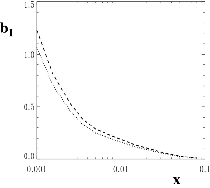
Fig. 7.1: Double scattering contribution to the tensor structure function $b_{1}$ from [70] . The dotted and dashed curves correspond to the Bonn [195] and Paris potential [152], respectively.

7.3.4 The ³He case

Although ${}^{3}{\mathrm{He}}$ would appear to be an ideal neutron target because of its large effective neutron polarization (7.5), the extraction of neutron spin structure functions nevertheless requires dealing with significant nuclear effects. We concentrate again on the structure function $g_{1}$ at small values of $x$. As for deuterium two types of corrections are relevant: higher angular momentum components of the ${}^{3}{\mathrm{He}}$ wave function lead to effective proton and neutron polarizations (7.5,7.6). Furthermore, the coherent interaction of the virtual photon with several nucleons causes shadowing. Accounting for both effects the neutron structure function can be deduced from $g_{1}^{{\mathrm{He}}}$ as follows:

$$g_{1}^{\mathrm{n}}\approx\frac{{\cal P}_{\mathrm{n}}^{{\mathrm{He}}}-\delta g_{1}^{{\mathrm{H}}e}/g_{1}^{\mathrm{n}}}{({\cal P}_{\mathrm{n}}^{{\mathrm{He}}})^{2}}\,g_{1}^{\mathrm{He}}-\frac{{\cal P}_{\mathrm{p}}^{{\mathrm{He}}}}{{\cal P}_{\mathrm{n}}^{{\mathrm{He}}}}\,g_{1}^{\mathrm{p}}.$$ (7.23)

Since $|{\cal P}_{\mathrm{p}}^{{\mathrm{He}}}|\ll|{\cal P}_{\mathrm{n}}^{{\mathrm{He}}}|$ the proton contribution in (7.23) is indeed suppressed.

Uncertainties in the effective nucleon polarizations which may influence the extraction of $g_{1}^{{\mathrm{n}}}$, result also from non-nucleonic degrees of freedom, e.g. mesons and $\mathchar 1\relax$-isobars, present in ³He. In Ref.[261] this is demonstrated for the non-singlet nucleon and ${\mathrm{A}}=3$ structure functions:

$$\mathchar 1\relax g_{1}^{{\mathrm{A}}=1}(x,Q^{2})=g_{1}^{{\mathrm{p}}}(x,Q^{2})-g_{1}^{{\mathrm{n}}}(x,Q^{2}),$$ (7.24)

$$\mathchar 1\relax g_{1}^{{\mathrm{A}}=3}(x,Q^{2})=g_{1}^{{\mathrm{H}}}(x,Q^{2})-g_{1}^{{\mathrm{He}}}(x,Q^{2}),$$ (7.25)

where $g_{1}^{\mathrm{H}}$ is the triton spin structure function. From the effective nucleon polarizations (7.5,7.6) and isospin symmetry of the three-body nuclear wave function one obtains:

$$\mathchar 1\relax g_{1}^{{\mathrm{A}}=3}=\left(1-\frac{4}{3}P_{{\mathrm{S}}^{\prime}}-\frac{2}{3}P_{{\mathrm{D}}}\right)\mathchar 1\relax g_{1}^{{\mathrm{A}}=1}.$$ (7.26)

Applying the Bjorken sum rule (2.66) to the ${\mathrm{A}}=1$ and ${\mathrm{A}}=3$ systems and taking their ratio leads to:

$$\frac{\intop_{0}^{1}dx\left[g_{1}^{\mathrm{He}}(x,Q^{2})-g_{1}^{\mathrm{H}}(x,Q^{2})\right]}{\intop_{0}^{1}dx\left[g_{1}^{n}(x,Q^{2})-g_{1}^{p}(x,Q^{2})\right]}=\frac{G_{A}(^{3}\mathrm{H})}{G_{A}(\mathrm{n})}.$$ (7.27)

The axial vector coupling constants $G_{A}(^{3}\mathrm{H})$ and $G_{A}(\mathrm{n})$ are measured in the $\beta$-decay of tritium and the neutron, respectively, with $G_{A}({\mathrm{n}})\equiv g_{A}=1.26$ [262]. If one considers incoherent scattering from individual nucleons and accounts only for the effective nucleon polarizations one finds from Eqs.(7.26,7.27):

$$\frac{G_{A}(^{3}\mathrm{H})}{g_{A}}=1-\frac{4}{3}P_{{\mathrm{S}}^{\prime}}-\frac{2}{3}P_{{\mathrm{D}}}=0.922\pm 0.006.$$ (7.28)

This result is however at variance with the empirical ratio ${G_{A}(^{3}\mathrm{H})}/{g_{A}}\approx 0.963\pm 0.003$ [263, 262]. One concludes that simply using effective nucleon polarizations from realistic three-nucleon calculations would lead to a violation of the Bjorken sum rule by approximately $4\%$ [261, 264]. On the other hand, it is known from nuclear $\beta$-decay and Gamov-Teller transitions that axial coupling constants in nuclei are renormalized by meson exchange currents and $\mathchar 1\relax$-isobars [265]. The possible influence of these non-nucleonic degrees of freedom on the extraction of $g_{1}^{{\mathrm{n}}}$ has to be carefully investigated [261].

At small values $x<0.1$ of the Bjorken variable, coherent multiple scattering from several nucleons in the target leads to the shadowing correction $\delta g_{1}$. Assuming again, as in Section 7.3.2, that the photon-nucleus scattering at small $x$ can be represented by the interaction of one effective hadronic fluctuation with invariant mass $M_{{\mathrm{X}}}^{2}\sim Q^{2}$, one finds [261]:

$$\frac{g_{1}^{{\mathrm{He}}}}{g_{1}^{\mathrm{n}}}\approx\left(2\,\frac{F_{2}^{{\mathrm{He}}}}{F_{2}^{\mathrm{N}}}-1\right),$$ (7.29)

i.e. shadowing in $g_{1}^{{\mathrm{He}}}$ is about twice as large as for the unpolarized structure function $F_{2}^{\mathrm{He}}$. This is also true for shadowing in the non-singlet structure function $\mathchar 1\relax g_{1}^{{\mathrm{A}}=3}$ [261]. A similar result has been found for the polarized deuterium case, see e.g. (7.21).

In Ref.[261] the shadowing correction (7.29) has been combined with the nuclear Bjorken sum rule (7.27). In the nuclear case, shadowing reduces the small-$x$ contribution to the Bjorken integral. Consequently the non-singlet nuclear structure function must be enhanced, i.e. $\mathchar 1\relax g_{1}^{{\mathrm{A}}=3}>\mathchar 1\relax g_{1}^{{\mathrm{A}}=1}$, somewhere in the region $x\,\mathrel{\raise 2.58334pt\hbox{$>$}\kern-7.7778pt\lower 2.79857pt\hbox{$\sim$}}\,0.1$. This is suggested to occur around $x\sim 0.1$, where the projectile may still interact with two nucleons inside the target. As a consequence a significant anti-shadowing is obtained in this kinematic region. The dynamical origin for such an enhancement is supposed to be independent of the flavor channel considered, so that this is also expected to occur for $g_{1}^{{\mathrm{He}}}$.

To summarize this discussion we emphasize that a precise extraction of the neutron spin structure function $g_{1}^{{\mathrm{n}}}$ from ${}^{3}{\mathrm{He}}$ data at $x\mathrel{\raise 2.58334pt\hbox{$<$}\kern-7.7778pt\lower 2.79857pt\hbox{$\sim$}}0.2$ requires a careful analysis of nuclear effects due to non-nucleonic (e.g. meson and $\mathchar 1\relax$-isobar) degrees of freedom in the ${}^{3}{\mathrm{He}}$ wave function and a detailed understanding of shadowing and anti-shadowing effects. The use of deuterium as a target may have advantages since non-nucleonic admixtures are supposed to be smaller due to weaker nuclear binding. Furthermore, especially at small $x$ the influence of shadowing on the extraction of $g_{1}^{{\mathrm{n}}}$ is less pronounced for deuterium as compared to ³He.

7.4 Polarized deep-inelastic scattering from nuclei at $x>0.2$

At moderate and large values of $x$, the distances probed by DIS from nuclei are smaller than $2$ fm as outlined in Section 4. Incoherent interactions of the virtual photon with hadronic constituents of the nucleus dominate, and the usual starting point is a description based on the impulse approximation including nucleon degrees of freedom only [213, 255, 266, 267]. This approach is not without question, but not much progress has so far been made beyond that level.

In the following we first discuss general features of the nuclear spin structure functions $g_{1}^{{\mathrm{A}}}$ and $g_{T}^{{\mathrm{A}}}=g_{1}^{{\mathrm{A}}}+g_{2}^{{\mathrm{A}}}$ in the framework of the impulse approximation. The nuclear target is treated non-relativistically. This allows, as in the unpolarized case, to factorize nucleon and nuclear degrees of freedom, introducing structure functions of nucleons as bound quasi-particles. The nuclear structure functions are then given as two-dimensional convolutions of the bound nucleon structure functions and the nucleon light-cone momentum distributions [213]:

$$g_{1}^{{\mathrm{A}}}(x) = \sum_{{i=1}}^{A}\intop\!dp^{2}\intop\limits_{x}\frac{dy}{y}\,D_{1}^{i}(y,p^{2})\,g_{1}^{i}\!\left(\frac{x}{y},p^{2}\right),$$ (7.30)

$$g_{T}^{{\mathrm{A}}}(x) = \sum_{{i=1}}^{A}\intop\!dp^{2}\intop\limits_{x}\frac{dy}{y}\,\left[D_{T}^{i}(y,p^{2})\,g_{T}^{i}\!\left(\frac{x}{y},p^{2}\right)+D_{T2}^{i}(y,p^{2})\,g_{2}^{{\mathrm{i}}}\!\left(\frac{x}{y},p^{2}\right)\right].$$ (7.31)

Here we have suppressed the $Q^{2}$-dependence for simplicity. The expressions in Eqs.(7.30, 7.31) resemble the result for the unpolarized nuclear structure function in Eq.(6.6): the exchanged virtual photon scatters from quarks which carry a fraction $x/y$ of the light-cone momentum of their parent nucleons, which in turn have a fraction $y=p^{+}/M$ of the nuclear light-cone momentum and a squared four-momentum $p^{2}$.

The nucleon distribution functions in Eqs.(7.30,7.31) are given by:

$$D_{1}(y,p^{2}) = \intop\!\frac{{{\mathrm{d}}}^{4}{p^{\prime}}}{(2\pi)^{4}}\ {\rm tr}\left[{\cal S}_{\|}(p^{\prime})\left(\widehat{\mathchar 6\relax}_{0}+\widehat{\mathchar 6\relax}_{z}\right)\right]\delta\left(y-\frac{p^{\prime+}}{M}\right)\delta\left(p^{2}-p^{\prime 2}\right),$$ (7.32)

$$D_{T}(y,p^{2}) = \intop\!\frac{{{\mathrm{d}}}^{4}p^{\prime}}{(2\pi)^{4}}\ {\rm tr}\left[{\cal S}_{\perp}(p^{\prime})\ \widehat{\mathchar 6\relax}_{\perp}\right]\delta\left(y-\frac{p^{\prime+}}{M}\right)\delta\left(p^{2}-p^{\prime 2}\right),$$ (7.33)

$$D_{T2}(y,p^{2}) = \intop\!\frac{{{\mathrm{d}}}^{4}{p^{\prime}}}{(2\pi)^{4}}\ {\rm tr}\left[{\cal S}_{\perp}(p^{\prime})\ \widehat{\cal T}_{2}\right]\delta\left(y-\frac{p^{\prime+}}{M}\right)\delta\left(p^{2}-p^{\prime 2}\right),$$ (7.34)

with the polarized nucleon spectral function:

$${\cal S}_{\sigma\sigma^{\prime}}(p)=2\pi\sum_{n}\delta\left(p_{0}-M-\varepsilon_{n}+T_{R}\right)\psi_{n,\sigma}({\mathchoice{\mbox{\boldmath$p$}}{\mbox{\boldmath$p$}}{\kern-0.20004pt\hbox{$\scriptstyle p$}\kern-3.52188pt\kern 0.39993pt\hbox{$\scriptstyle p$}\kern-3.52188pt\kern-0.20004pt\raise 0.21698pt\hbox{$\scriptstyle p$}}{\kern-0.20004pt\hbox{$\scriptscriptstyle p$}\kern-2.51563pt\kern 0.39993pt\hbox{$\scriptscriptstyle p$}\kern-2.51563pt\kern-0.20004pt\raise 0.21698pt\hbox{$\scriptscriptstyle p$}}})\psi^{*}_{n,\sigma^{\prime}}({\mathchoice{\mbox{\boldmath$p$}}{\mbox{\boldmath$p$}}{\kern-0.20004pt\hbox{$\scriptstyle p$}\kern-3.52188pt\kern 0.39993pt\hbox{$\scriptstyle p$}\kern-3.52188pt\kern-0.20004pt\raise 0.21698pt\hbox{$\scriptstyle p$}}{\kern-0.20004pt\hbox{$\scriptscriptstyle p$}\kern-2.51563pt\kern 0.39993pt\hbox{$\scriptscriptstyle p$}\kern-2.51563pt\kern-0.20004pt\raise 0.21698pt\hbox{$\scriptscriptstyle p$}}}).$$ (7.35)

Here the summation is performed over the complete set of states with $A-1$ nucleons. The functions $\psi_{n,\sigma}({\mathchoice{\mbox{\boldmath$p$}}{\mbox{\boldmath$p$}}{\kern-0.20004pt\hbox{$\scriptstyle p$}\kern-3.52188pt\kern 0.39993pt\hbox{$\scriptstyle p$}\kern-3.52188pt\kern-0.20004pt\raise 0.21698pt\hbox{$\scriptstyle p$}}{\kern-0.20004pt\hbox{$\scriptscriptstyle p$}\kern-2.51563pt\kern 0.39993pt\hbox{$\scriptscriptstyle p$}\kern-2.51563pt\kern-0.20004pt\raise 0.21698pt\hbox{$\scriptscriptstyle p$}}})=\left\langle({\mathrm{A}}-1)_{n},-{\mathchoice{\mbox{\boldmath$p$}}{\mbox{\boldmath$p$}}{\kern-0.20004pt\hbox{$\scriptstyle p$}\kern-3.52188pt\kern 0.39993pt\hbox{$\scriptstyle p$}\kern-3.52188pt\kern-0.20004pt\raise 0.21698pt\hbox{$\scriptstyle p$}}{\kern-0.20004pt\hbox{$\scriptscriptstyle p$}\kern-2.51563pt\kern 0.39993pt\hbox{$\scriptscriptstyle p$}\kern-2.51563pt\kern-0.20004pt\raise 0.21698pt\hbox{$\scriptscriptstyle p$}}}|\psi_{\sigma}(0)|{\mathrm{A}}\right\rangle$ are the probability amplitudes to find a nucleon with polarization $\sigma$ in the nuclear ground state and the remaining $A-1$ nucleons in a state $n$ with total momentum $-{\mathchoice{\mbox{\boldmath$p$}}{\mbox{\boldmath$p$}}{\kern-0.20004pt\hbox{$\scriptstyle p$}\kern-3.52188pt\kern 0.39993pt\hbox{$\scriptstyle p$}\kern-3.52188pt\kern-0.20004pt\raise 0.21698pt\hbox{$\scriptstyle p$}}{\kern-0.20004pt\hbox{$\scriptscriptstyle p$}\kern-2.51563pt\kern 0.39993pt\hbox{$\scriptscriptstyle p$}\kern-2.51563pt\kern-0.20004pt\raise 0.21698pt\hbox{$\scriptscriptstyle p$}}}$. The separation energy $\varepsilon_{n}$ and the recoil energy of the residual nuclear system $T_{R}$ enter in Eq.(7.35) as for the unpolarized case (6.5). For $g_{1}$ the target nucleus is chosen to be polarized parallel to the photon momentum as indicated in Eq.(7.32) by the subscript $\|$. For the transverse structure function $g_{T}$ the target polarization is taken perpendicular to the momentum transfer and denoted by $\perp$.

The nucleon spin operators which multiply the spectral functions in Eqs.(7.32,7.33,7.34) refer to the active nucleon. They read:

$$\widehat{\mathchar 6\relax}_{0} = \frac{\mathchoice{\mbox{\boldmath$\sigma$}}{\mbox{\boldmath$\sigma$}}{\kern-0.20004pt\hbox{$\scriptstyle\sigma$}\kern-3.9999pt\kern 0.39993pt\hbox{$\scriptstyle\sigma$}\kern-3.9999pt\kern-0.20004pt\raise 0.21698pt\hbox{$\scriptstyle\sigma$}}{\kern-0.20004pt\hbox{$\scriptscriptstyle\sigma$}\kern-2.85706pt\kern 0.39993pt\hbox{$\scriptscriptstyle\sigma$}\kern-2.85706pt\kern-0.20004pt\raise 0.21698pt\hbox{$\scriptscriptstyle\sigma$}}\cdot\mathchoice{\mbox{\boldmath$p$}}{\mbox{\boldmath$p$}}{\kern-0.20004pt\hbox{$\scriptstyle p$}\kern-3.52188pt\kern 0.39993pt\hbox{$\scriptstyle p$}\kern-3.52188pt\kern-0.20004pt\raise 0.21698pt\hbox{$\scriptstyle p$}}{\kern-0.20004pt\hbox{$\scriptscriptstyle p$}\kern-2.51563pt\kern 0.39993pt\hbox{$\scriptscriptstyle p$}\kern-2.51563pt\kern-0.20004pt\raise 0.21698pt\hbox{$\scriptscriptstyle p$}}}{M},\quad\quad\quad\quad\widehat{\mathchar 6\relax}_{j}=\left(1-\frac{{\mathchoice{\mbox{\boldmath$p$}}{\mbox{\boldmath$p$}}{\kern-0.20004pt\hbox{$\scriptstyle p$}\kern-3.52188pt\kern 0.39993pt\hbox{$\scriptstyle p$}\kern-3.52188pt\kern-0.20004pt\raise 0.21698pt\hbox{$\scriptstyle p$}}{\kern-0.20004pt\hbox{$\scriptscriptstyle p$}\kern-2.51563pt\kern 0.39993pt\hbox{$\scriptscriptstyle p$}\kern-2.51563pt\kern-0.20004pt\raise 0.21698pt\hbox{$\scriptscriptstyle p$}}}^{2}}{2M^{2}}\right)\sigma_{j}+\frac{\mathchoice{\mbox{\boldmath$\sigma$}}{\mbox{\boldmath$\sigma$}}{\kern-0.20004pt\hbox{$\scriptstyle\sigma$}\kern-3.9999pt\kern 0.39993pt\hbox{$\scriptstyle\sigma$}\kern-3.9999pt\kern-0.20004pt\raise 0.21698pt\hbox{$\scriptstyle\sigma$}}{\kern-0.20004pt\hbox{$\scriptscriptstyle\sigma$}\kern-2.85706pt\kern 0.39993pt\hbox{$\scriptscriptstyle\sigma$}\kern-2.85706pt\kern-0.20004pt\raise 0.21698pt\hbox{$\scriptscriptstyle\sigma$}}\cdot\mathchoice{\mbox{\boldmath$p$}}{\mbox{\boldmath$p$}}{\kern-0.20004pt\hbox{$\scriptstyle p$}\kern-3.52188pt\kern 0.39993pt\hbox{$\scriptstyle p$}\kern-3.52188pt\kern-0.20004pt\raise 0.21698pt\hbox{$\scriptstyle p$}}{\kern-0.20004pt\hbox{$\scriptscriptstyle p$}\kern-2.51563pt\kern 0.39993pt\hbox{$\scriptscriptstyle p$}\kern-2.51563pt\kern-0.20004pt\raise 0.21698pt\hbox{$\scriptscriptstyle p$}}}{2M^{2}}\ p_{j},$$

$$\widehat{\cal T}_{2} = -{{\mathchoice{\mbox{\boldmath$p$}}{\mbox{\boldmath$p$}}{\kern-0.20004pt\hbox{$\scriptstyle p$}\kern-3.52188pt\kern 0.39993pt\hbox{$\scriptstyle p$}\kern-3.52188pt\kern-0.20004pt\raise 0.21698pt\hbox{$\scriptstyle p$}}{\kern-0.20004pt\hbox{$\scriptscriptstyle p$}\kern-2.51563pt\kern 0.39993pt\hbox{$\scriptscriptstyle p$}\kern-2.51563pt\kern-0.20004pt\raise 0.21698pt\hbox{$\scriptscriptstyle p$}}}_{\perp}\cdot{\mathchoice{\mbox{\boldmath$S$}}{\mbox{\boldmath$S$}}{\kern-0.20004pt\hbox{$\scriptstyle S$}\kern-4.69582pt\kern 0.39993pt\hbox{$\scriptstyle S$}\kern-4.69582pt\kern-0.20004pt\raise 0.21698pt\hbox{$\scriptstyle S$}}{\kern-0.20004pt\hbox{$\scriptscriptstyle S$}\kern-3.35414pt\kern 0.39993pt\hbox{$\scriptscriptstyle S$}\kern-3.35414pt\kern-0.20004pt\raise 0.21698pt\hbox{$\scriptscriptstyle S$}}}_{\perp}\over M}\left(\frac{\mathchoice{\mbox{\boldmath$\sigma$}}{\mbox{\boldmath$\sigma$}}{\kern-0.20004pt\hbox{$\scriptstyle\sigma$}\kern-3.9999pt\kern 0.39993pt\hbox{$\scriptstyle\sigma$}\kern-3.9999pt\kern-0.20004pt\raise 0.21698pt\hbox{$\scriptstyle\sigma$}}{\kern-0.20004pt\hbox{$\scriptscriptstyle\sigma$}\kern-2.85706pt\kern 0.39993pt\hbox{$\scriptscriptstyle\sigma$}\kern-2.85706pt\kern-0.20004pt\raise 0.21698pt\hbox{$\scriptscriptstyle\sigma$}}\cdot\mathchoice{\mbox{\boldmath$p$}}{\mbox{\boldmath$p$}}{\kern-0.20004pt\hbox{$\scriptstyle p$}\kern-3.52188pt\kern 0.39993pt\hbox{$\scriptstyle p$}\kern-3.52188pt\kern-0.20004pt\raise 0.21698pt\hbox{$\scriptstyle p$}}{\kern-0.20004pt\hbox{$\scriptscriptstyle p$}\kern-2.51563pt\kern 0.39993pt\hbox{$\scriptscriptstyle p$}\kern-2.51563pt\kern-0.20004pt\raise 0.21698pt\hbox{$\scriptscriptstyle p$}}}{M}+\sigma_{z}\left(1-\frac{p_{z}}{M}\right)\right),$$ (7.36)

where $j$ denotes spatial indices. Furthermore, ${\mathchoice{\mbox{\boldmath$p$}}{\mbox{\boldmath$p$}}{\kern-0.20004pt\hbox{$\scriptstyle p$}\kern-3.52188pt\kern 0.39993pt\hbox{$\scriptstyle p$}\kern-3.52188pt\kern-0.20004pt\raise 0.21698pt\hbox{$\scriptstyle p$}}{\kern-0.20004pt\hbox{$\scriptscriptstyle p$}\kern-2.51563pt\kern 0.39993pt\hbox{$\scriptscriptstyle p$}\kern-2.51563pt\kern-0.20004pt\raise 0.21698pt\hbox{$\scriptscriptstyle p$}}}_{\perp}$ is the transverse component of the nucleon three-momentum, ${\mathchoice{\mbox{\boldmath$p$}}{\mbox{\boldmath$p$}}{\kern-0.20004pt\hbox{$\scriptstyle p$}\kern-3.52188pt\kern 0.39993pt\hbox{$\scriptstyle p$}\kern-3.52188pt\kern-0.20004pt\raise 0.21698pt\hbox{$\scriptstyle p$}}{\kern-0.20004pt\hbox{$\scriptscriptstyle p$}\kern-2.51563pt\kern 0.39993pt\hbox{$\scriptscriptstyle p$}\kern-2.51563pt\kern-0.20004pt\raise 0.21698pt\hbox{$\scriptscriptstyle p$}}}=({\mathchoice{\mbox{\boldmath$p$}}{\mbox{\boldmath$p$}}{\kern-0.20004pt\hbox{$\scriptstyle p$}\kern-3.52188pt\kern 0.39993pt\hbox{$\scriptstyle p$}\kern-3.52188pt\kern-0.20004pt\raise 0.21698pt\hbox{$\scriptstyle p$}}{\kern-0.20004pt\hbox{$\scriptscriptstyle p$}\kern-2.51563pt\kern 0.39993pt\hbox{$\scriptscriptstyle p$}\kern-2.51563pt\kern-0.20004pt\raise 0.21698pt\hbox{$\scriptscriptstyle p$}}}_{\perp},p_{z})$, and ${\mathchoice{\mbox{\boldmath$S$}}{\mbox{\boldmath$S$}}{\kern-0.20004pt\hbox{$\scriptstyle S$}\kern-4.69582pt\kern 0.39993pt\hbox{$\scriptstyle S$}\kern-4.69582pt\kern-0.20004pt\raise 0.21698pt\hbox{$\scriptstyle S$}}{\kern-0.20004pt\hbox{$\scriptscriptstyle S$}\kern-3.35414pt\kern 0.39993pt\hbox{$\scriptscriptstyle S$}\kern-3.35414pt\kern-0.20004pt\raise 0.21698pt\hbox{$\scriptscriptstyle S$}}}_{\perp}$ determines the transverse spin quantization axis relative to the photon momentum which is taken along the $z$-direction.

From Eqs.(7.30,7.31) we observe that $g_{1}^{{\mathrm{A}}}$ is expressed entirely in terms of the corresponding nucleon structure function $g_{1}^{{\mathrm{N}}}$. This is different for $g_{T}^{{\mathrm{A}}}$ which receives contributions from $g_{T}^{{\mathrm{N}}}$ as well as from $g_{2}^{{\mathrm{N}}}$.

If the bound nucleon structure functions in Eqs.(7.30,7.31) are replaced by free ones, one ends up with the conventional one-dimensional convolution ansatz for nuclear structure functions [213, 255]. Relativistic contributions which lead beyond the convolution formula (7.30,7.31) have been investigated in Refs.[268, 269], and corrections have been estimated within a quark-diquark model for the bound nucleon. Deviations from non-relativistic convolution were generally found to be small, except at very large $x>0.9$.

Given that the nuclear spectral functions, polarized as well as unpolarized, receive their major contributions from small nucleon momenta, systematic expansions of $g_{1}^{{\mathrm{A}}}$ and $g_{T}^{{\mathrm{A}}}$ for $x<0.7$ can be performed around $y=1$ and the mass-shell point $p^{2}=M^{2}$, keeping terms of order $\varepsilon/M$ and $\mathchoice{\mbox{\boldmath$p$}}{\mbox{\boldmath$p$}}{\kern-0.20004pt\hbox{$\scriptstyle p$}\kern-3.52188pt\kern 0.39993pt\hbox{$\scriptstyle p$}\kern-3.52188pt\kern-0.20004pt\raise 0.21698pt\hbox{$\scriptstyle p$}}{\kern-0.20004pt\hbox{$\scriptscriptstyle p$}\kern-2.51563pt\kern 0.39993pt\hbox{$\scriptscriptstyle p$}\kern-2.51563pt\kern-0.20004pt\raise 0.21698pt\hbox{$\scriptscriptstyle p$}}^{2}/M^{2}$. Results and applications to spin structure functions of the deuteron and ³He are discussed in Refs.[213, 255, 267, 270]. As a general rule, the structure functions at $x<0.7$ are well described using simply the effective nucleon polarizations (7.4,7.5,7.6).

8 Further developments and perspectives

We close this review with a short summary of the key physics points together with an outlook on several selected topics for which investigations are still actively under way. We comment on exclusive vector meson production from nuclei, questions of shadowing at large $Q^{2}$ and the issue of high parton densities in nuclear systems.

8.1 Coherence effects in DIS and in the exclusive electroproduction of vector mesons

Nuclear shadowing in inclusive deep-inelastic lepton scattering is a prime source of information on coherently propagating hadronic or quark-gluon fluctuations of the virtual photon in a nuclear medium. By selecting different kinematic cuts in $Q^{2}$ and energy transfer $\nu$, one can focus on different components of the photon’s Fock space wave function. An even more stringent selection of such components can be achieved in exclusive photo- and electroproduction processes, and in particular in high-energy diffractive vector meson production. Data on vector meson production from nuclei have become available in recent years at FNAL (E665) [271], CERN (NMC) [272, 273], and DESY (HERMES) [274], and further experiments are under discussion at TJNAF [275] and DESY (HERA, HERMES) [254].

Depending on energy and momentum transfer, the mechanism of vector meson formation can be quite different. In the range $\nu>3$ GeV and $Q^{2}\,\mathrel{\raise 2.58334pt\hbox{$<$}\kern-7.7778pt\lower 2.79857pt\hbox{$\sim$}}\,1$ GeV² the production process is well described using the vector meson dominance picture (see e.g. [25]): in the lab frame the photon converts into a vector meson prior to scattering from the target. On the other hand, at large $Q^{2}\gg 1$ GeV² perturbative QCD calculations show that the photon-nucleon interaction produces an initially small-sized, color singlet quark-antiquark wave packet [166, 276]. At high photon energies the finally observed vector meson is then formed at a much later stage.

The transition from small to large $Q^{2}$ interpolates between non-perturbative hadron formation and perturbative quark-antiquark-gluon dynamics, a question of central importance in QCD. Nuclear targets are particular helpful at this point because they serve as analyzers for the coherent interaction of the produced $q\bar{q}$-gluon system with several nucleons [277]. The distance between two nucleons provides the “femtometer stick” which can be used to measure the relevant coherence lengths (for reviews and references see [278, 279, 280]).

The characteristic scales for this discussion have been encountered several times in previous sections. First, there is the typical longitudinal distance (propagation length)

$$\lambda\approx\frac{2\nu}{m^{2}+Q^{2}}\,.$$ (8.1)

It represents the distance over which a hadronic fluctuation of invariant mass $m$ propagates in the lab frame when induced by a photon of energy $\nu$ and virtuality $Q^{2}$. At large $Q^{2}$ the initially produced wave packet is characterized by its transverse size $b$. For longitudinally polarized photons,

$$b=\frac{const}{Q}.$$ (8.2)

In perturbative QCD the minimal Fock space component has $const\sim 4$–$5$ at $Q^{2}\mathrel{\raise 2.58334pt\hbox{$>$}\kern-7.7778pt\lower 2.79857pt\hbox{$\sim$}}5\,{\mathrm{GeV}}^{2}$ [166, 281]. Thus for $Q^{2}=5\,{\mathrm{GeV}}^{2}$ and $const=4$, the transverse size of the initial wave packet is $b\sim 0.4$ fm, a small fraction of the diameter of a fully developed $\rho$ meson.

Recent measurements at HERMES [274] have observed effects related to the coherence length $\lambda$ in $\rho^{0}$ electroproduction on hydrogen, deuterium, ³He, and ¹⁴N. The range of energy and momentum transfers covered by the experiment is $9\,{\mathrm{GeV}}<\nu<20\,{\mathrm{GeV}}$ and $0.4\,{\mathrm{GeV}}^{2}<Q^{2}<5\,{\mathrm{GeV}}^{2}$. This implies coherence lengths in the range $0.6\,{\mathrm{fm}}\,\mathrel{\raise 2.58334pt\hbox{$<$}\kern-7.7778pt\lower 2.79857pt\hbox{$\sim$}}\,\lambda<8\,{\mathrm{fm}}$ covering scales from individual nucleons up to and beyond nuclear dimensions. (The interesting upper section of the available $Q^{2}$ interval, $Q^{2}\,\mathrel{\raise 2.58334pt\hbox{$>$}\kern-7.7778pt\lower 2.79857pt\hbox{$\sim$}}\,4$ GeV², has been accessible only for small energies with $\nu$ with $\lambda\,\mathrel{\raise 2.58334pt\hbox{$<$}\kern-7.7778pt\lower 2.79857pt\hbox{$\sim$}}\,1$ fm in these measurements.)

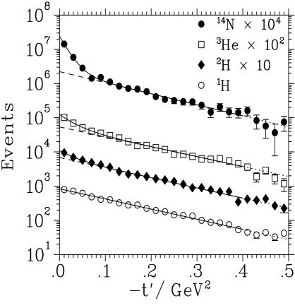
Fig. 8.1: The rates of produced $\rho^{0}$’s plotted against $t^{\prime}=t-t_{0}$ for hydrogen, deuterium, ³He, and ¹⁴N. The solid lines show fits to the data, the dashed lines are inferred incoherent contributions (for details see Ref.[274]).

Given the four-momenta $q$ and $k$ of the incoming virtual photon and the produced $\rho$ meson, the $t$-channel momentum transfer to the nucleon is $t=(q-k)^{2}$. In Fig.8.1 the rate of produced $\rho^{0}$’s is plotted against $t^{\prime}=t-t_{0}$, the squared momentum transfer above threshold ($|t_{0}|\simeq\lambda^{-2}$). At $|t^{\prime}|\ll 0.1$ GeV² coherent production dominates, leaving the nucleus as a whole in the ground state. Such coherent processes fall off rapidly with the nuclear form factor, so that at $|t^{\prime}|\,\mathrel{\raise 2.58334pt\hbox{$>$}\kern-7.7778pt\lower 2.79857pt\hbox{$\sim$}}\,0.1$ GeV² mostly incoherent $\rho$ production from individual nucleons remains.

Consider now the incoherent production of vector mesons from nuclei. In the absence of coherent rescattering processes the nuclear $\rho$ production cross section $\sigma_{{\mathrm{A}}}$ would simply be $A$ times the production cross section $\sigma_{{\mathrm{N}}}$ on a free nucleon. Nuclear effects are conveniently discussed in terms of the transparency ratio, $T_{{\mathrm{A}}}=\sigma_{{\mathrm{A}}}/({A}\sigma_{{\mathrm{N}}})$. The measured ratio for ¹⁴N is plotted as a function of the longitudinal propagation length $\lambda$ in Fig.8.2. The deviation of $T_{{\mathrm{A}}}$ from unity for $\lambda\,\mathrel{\raise 2.58334pt\hbox{$<$}\kern-7.7778pt\lower 2.79857pt\hbox{$\sim$}}\,1$ fm simply reflects the “trivial” final state rescattering of the $\rho$ meson after being produced on one of the nucleons. More interesting effects are visible when $\lambda$ exceeds the average nucleon-nucleon distance of about $2$ fm. Now the hadronic fluctuations of the photon can scatter coherently on several nucleons also prior to the production of the final state vector meson, and the transparency ratio $T_{{\mathrm{A}}}$ systematically decreases until it exceeds the nuclear diameter. The dashed curve in Fig.8.2 shows a theoretical prediction calculated within the vector meson dominance model [282]. Its agreement with data suggests that the production process is dominated, given the relatively low $Q^{2}$ involved, by hadronic fluctuations which interact about as strongly as the produced $\rho$ meson. Further systematic investigations of such coherence length effects, especially its detailed dependence on the momentum transfer $t$, are discussed at TJNAF [275, 283].

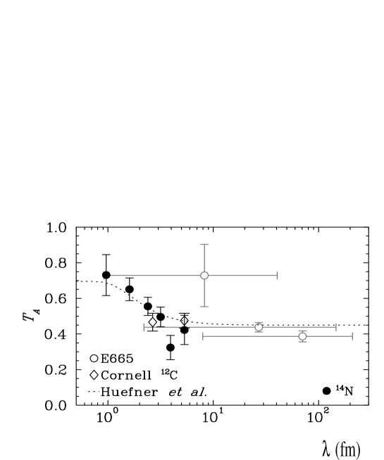
Fig. 8.2: The nuclear transparency $T_{{\mathrm{A}}}$ as a function of the propagation length $\lambda$ for ¹⁴N. HERMES data [274] are indicated by full dots. The open symbols represent data from previous experiments [284, 271]. The dashed curve shows a Glauber calculation from Ref.[282]

It is interesting to push these observations to more extreme regions of very large $Q^{2}$ and $\nu$. Once the energy transfer exceeds several tens of GeV, a further scale enters. At large $Q^{2}$ the $q\bar{q}$ fluctuation of the photon starts out initially as a small-sized wave packet. The time it takes for this wave packet to develop into the final vector meson is called the formation time $\tau_{f}$ [278, 279, 280]. To be specific, let the observed vector meson again be a $\rho^{0}$. The small initial wave packet is generally not an eigenstate of the strong interaction Hamiltonian. Now consider expanding the wave packet in hadronic eigenstates. Clearly, for a wave packet with a size small compared to typical hadronic dimensions, several such eigenstates are necessary to represent the wave function of the packet. Let one of those hadronic eigenstates in the expansion be the $\rho$ meson itself (mass $m_{\rho}$), let another one be a neighboring state with larger mass (say, $m_{\rho^{\prime}}=m_{\rho}+\delta m$). The characteristic propagation length of the $\rho$ component of the $q\bar{q}$-gluon wave packet is $\lambda\simeq 2\nu/(m_{\rho}^{2}+Q^{2})$, that of the neighboring state is $\lambda^{\prime}\simeq 2\nu/(m_{\rho}^{2}+Q^{2}+2m_{\rho}\,\delta m)$. The phase difference between both states is determined by their wave numbers $1/\lambda$ and $1/\lambda^{\prime}$. The time it takes to filter out all but the $\rho$ meson component when passing through the nucleus is then

$$\tau_{f}\sim\frac{\nu}{m_{\rho}\,\delta m}\,.$$ (8.3)

Thus when $\nu$ is sufficiently large so that $\tau_{f}$ reaches nuclear dimensions and $Q^{2}$ is large, a small-sized $q\bar{q}$ wave packet induced by the photon has a chance to travel over large distances inside nuclei and interact weakly, its cross section being proportional to $b^{2}\sim 1/Q^{2}$.

This phenomenon is commonly named color coherence or color (singlet) transparency [277, 278, 279, 280]. It has been addressed in exclusive vector meson production experiments at FNAL (E665) [271] and CERN (NMC) [273]. The interpretation of data in terms of color transparency is still under debate (see e.g. [285, 286]). Possible future developments with nuclei at HERA [254] could offer an enormous extension of the accessible kinematic range.

8.2 Nuclear shadowing in DIS at large $Q^{2}$

Experimental information on nuclear shadowing in inclusive DIS is available, up to now, only from fixed target experiments, with the kinematic range restricted to $Q^{2}\,\mathrel{\raise 2.58334pt\hbox{$<$}\kern-7.7778pt\lower 2.79857pt\hbox{$\sim$}}\,1$ GeV² at $x\ll 0.1$. Although there are currently no data on nuclear shadowing at large $Q^{2}\gg 1$ GeV², it is nevertheless instructive to investigate what one should expect in comparison with the previous results at smaller $Q^{2}$. Such a study is possible due to recent data on diffractive production from the HERA collider and has been performed in Refs.[147, 287, 288].

One finds that contributions from vector mesons are negligible at large momentum transfers since diffractive vector meson production is strongly suppressed at $Q^{2}>10$ GeV². Furthermore, the ZEUS data [52] on the ratio of diffractive to total photon-nucleon cross sections (Fig.2.8) suggest that diffractively produced states with large mass are relevant at large $Q^{2}$. Therefore at large $Q^{2}$ shadowing probes the coherent interaction of quark-gluon configurations with large invariant mass. This is complementary to fixed target experiments at FNAL (E665) and CERN (NMC) where the coherent interaction of low mass vector mesons played a dominant role (see Sections 5.1.4 and 5.4).

In Section 5.2 we have argued that to leading order in $1/Q^{2}$ shadowing is dominated by the interaction of large-size hadronic fluctuations of the exchanged photon. This suggests a weak energy dependence of nuclear shadowing. However, at very small $x$ together with very large $Q^{2}$, the steadily growing number of partons in the photon-nucleon system makes quark-gluon configurations of the photon interact like ordinary hadrons, even if they have small transverse size proportional to $1/Q^{2}$ (see e.g. Eq.(5.33)). As a consequence one expects a more rapid energy dependence of shadowing as compared to the case of small $Q^{2}$. On similar grounds the diffractive leptoproduction cross section at $x\ll 0.1$ and $Q^{2}\gg 1$ GeV² should rise more strongly than suggested by Regge phenomenology. Possible indications for this behavior have been found at HERA [50, 52], signaling the onset of a new kinematic regime with a complex interplay between soft (large size) and hard (small size) partonic components of the interacting photon. A systematic investigation of strong interaction dynamics in this kinematic region is a major challenge. Here electron-nucleus collider experiments could give important new insights [254].

8.3 Physics of high parton densities

An elementary QCD treatment of radiative corrections in nucleon and nuclear structure functions, or equivalently, in quark and gluon distributions is provided by the DGLAP evolution equations (see Section 2.4). In leading logarithmic approximation one sums over $\alpha_{s}\ln Q^{2}/\mathchar 3\relax^{2}$ terms, each of which represents a quark radiating a gluon or a gluon splitting into a $q\bar{q}$ or gluon pair. A contribution $(\alpha_{s}\ln Q^{2}/\mathchar 3\relax^{2})^{n}$ is associated with the radiation from $n$ partons in a physical gauge. Due to radiation partons loose momentum. Therefore DGLAP evolution leads to a rise of quark and gluon distribution functions at small $x$: strongly increasing numbers of partons carry smaller and smaller fractions of the total momentum. For example, consider gluons which dominate the dynamics of parton distributions at small $x$. Suppose that we are given an initial gluon distribution, prior to radiative QCD corrections, at a momentum scale $Q_{0}^{2}$. This initial distribution can be non-singular (finite) at $x\to 0$. Now turn on QCD radiation and DGLAP evolution. The resulting asymptotic behavior of the gluon distribution function at $x\ll 1$ and large $Q^{2}$ is (see e.g. [289]):

$$xg(x,Q^{2})\sim\exp\left\{\frac{12}{5}\sqrt{\ln\left(\frac{\ln(Q^{2}/\mathchar 3\relax^{2})}{\ln(Q_{0}^{2}/\mathchar 3\relax^{2})}\right)\ln(1/x)}\right\}.$$ (8.4)

One observes a strong rise of $xg(x,Q^{2})$ at $x\ll 1$. This increase of the gluon density with decreasing $x$ can however not continue indefinitely. At very small $x$ the density of gluons becomes so large that they interact with each other reducing their density through annihilation. Thus one enters a new regime of very high parton densities where standard methods of perturbation theory are inappropriate despite small values for the coupling $\alpha_{s}$, and resummation techniques to infinite order have to be applied (for references see e.g. [134, 135, 136, 137, 138, 139]).

For further illustration let us view the scattering process in a frame where the target momentum is very large, $P=|\mathchoice{\mbox{\boldmath$P$}}{\mbox{\boldmath$P$}}{\kern-0.20004pt\hbox{$\scriptstyle P$}\kern-5.46632pt\kern 0.39993pt\hbox{$\scriptstyle P$}\kern-5.46632pt\kern-0.20004pt\raise 0.21698pt\hbox{$\scriptstyle P$}}{\kern-0.20004pt\hbox{$\scriptscriptstyle P$}\kern-3.90451pt\kern 0.39993pt\hbox{$\scriptscriptstyle P$}\kern-3.90451pt\kern-0.20004pt\raise 0.21698pt\hbox{$\scriptscriptstyle P$}}|\rightarrow\infty$. A measurement at specific values of $Q^{2}$ and $x$ probes partons over a longitudinal distance $\mathchar 1\relax z\sim 1/(Px)$ and with a transverse size $\mathchar 1\relax b\sim 1/\sqrt{Q^{2}}$. Thus at small values of $x$ and moderate $Q^{2}$ parton wave functions overlap, leading to high parton densities, so that the rate of parton-parton annihilation processes increases. This rate involves the probability of finding at least two partons per unit area in the nucleon [289, 290]. In this respect parton recombination can be regarded as a “non-linear” correction to radiation processes described by standard DGLAP evolution, where parton distribution functions enter linearly (see e.g. Eq.(2.39)).

The existing HERA data on free nucleon structure functions at $Q^{2}\,\mathrel{\raise 2.58334pt\hbox{$>$}\kern-7.7778pt\lower 2.79857pt\hbox{$\sim$}}\,1$ GeV² and $x\,\mathrel{\raise 2.58334pt\hbox{$>$}\kern-7.7778pt\lower 2.79857pt\hbox{$\sim$}}\,10^{-4}$ do not show a clear sign for the need of additional parton fusion corrections in the evolution equations (see e.g. [9]). However, phenomena related to high parton densities at small $x$ should be magnified in nuclei since nuclear parton densities are enhanced. For example, if shadowing is ignored and the nuclear gluon distribution is assumed to be the sum of the gluon distributions of individual nucleons, $g_{{\mathrm{A}}}(x,Q^{2})={A}\,g_{{\mathrm{N}}}(x,Q^{2})$, then the ratio of gluon densities in a nucleus and a nucleon per (transverse) area is [291]:

$$\left.\frac{g_{{\mathrm{A}}}(x,Q^{2})}{\pi R_{{\mathrm{A}}}^{2}}\right/\frac{g_{{\mathrm{N}}}(x,Q^{2})}{\pi r_{{\mathrm{N}}}^{2}}\approx\frac{{{\mathrm{A}}}\,r_{{\mathrm{N}}}^{2}}{R_{{\mathrm{A}}}^{2}}\approx\,0.5\,{{\mathrm{A}}}^{1/3},$$ (8.5)

where $r_{{\mathrm{N}}}\approx 0.8\,\rm{fm}$ and $R_{{\mathrm{A}}}\approx r_{0}A^{1/3}\approx 1.1\,{\rm fm}\,{{\mathrm{A}}}^{1/3}$ have been used for nucleon and nuclear radii, respectively. Effects beyond DGLAP evolution should therefore be amplified in nuclei and set in already at a larger value of $x$ as compared to free nucleons.

In Ref.[290, 292] corrections to DGLAP evolution for nuclear parton distributions have been calculated in the leading logarithmic approximation taking into account corrections due to parton-parton recombination. The nuclear gluon distribution is written in two parts: $x\,g_{{\mathrm{A}}}(x,Q^{2})=x\,{\mathrm{A}}\,g_{{\mathrm{N}}}(x,Q^{2})+\delta\left(\,x\,g_{{\mathrm{A}}}(x,Q^{2})\right)$. The first term is associated with independent nucleons and evolves accordingly. The second term is the correction of interest here and describes the interaction of gluons from different nucleons. Its evolution due to gluon-gluon recombination reads [290, 292]:

$$Q^{2}\frac{\partial}{\partial Q^{2}}\frac{\delta\left(\,x\,g_{{\mathrm{A}}}(x,Q^{2})\right)}{{{\mathrm{A}}}}=-\frac{81}{16}\frac{{{\mathrm{A}}}^{1/3}}{Q^{2}\,r_{0}^{2}}\,\alpha_{s}^{2}(Q^{2})\intop_{x}^{1}\frac{dx^{\prime}}{x^{\prime}}\left[x^{\prime}g_{{\mathrm{N}}}(x^{\prime},Q^{2})\right]^{2}.$$ (8.6)

Clearly gluon-gluon recombination is enhanced in nuclei. One finds [293, 294] that the $x$-range where non-linear effects (8.6) become significant, differs for heavy nuclei and free nucleons by more than two orders of magnitude, assuming $xg_{{\mathrm{N}}}(x)\sim x^{-0.2}$.

Investigations of unitarity constraints in hard two-body amplitudes [166] also suggest that non-linear effects at high parton densities can be significant in nuclei at $Q^{2}\sim 10$ GeV² and $x\sim 10^{-4}$.

While the kinematic bounds for the applicability of “normal” DGLAP evolution are quite well defined, the dynamical mechanisms responsible for slowing down the rapid increase of parton distributions at large $Q^{2}$ and very small $x$ are not yet clear. One is entering a new domain of QCD, dealing with partonic systems of high density, which presents new challenges.

Acknowledgments

We gratefully acknowledge many discussions and conversations with S. Brodsky, L. Frankfurt, P. Hoyer, B. Kopeliovich, S. Kulagin, L. Mankiewicz, W. Melnitchouk, G.A. Miller, N. Nikolaev, K. Rith, M. Sargsian, M. Strikman, A.W. Thomas and M. Vänttinen.

References

- [1] L.L. Frankfurt and M.I. Strikman, Phys. Rept. 160 (1988) 235.
- [2] R.L. Jaffe, Relativistic Dynamics and Quark Nuclear Physics, edited by M.B. Johnson and A. Picklesimer, Wiley, New York, USA, 1986.
- [3] R.P. Bickerstaff and A.W. Thomas, J. Phys. G15 (1989) 1523.
- [4] M. Arneodo, Phys. Rept. 240 (1994) 301.
- [5] D.F. Geesaman, K. Saito and A.W. Thomas, Ann. Rev. Nucl. Part. Sci. 45 (1995) 337.
- [6] R.G. Roberts, The Structure of the Proton: Deep Inelastic Scattering (Cambridge University Press, Cambridge, UK, 1990).
- [7] T. Muta, Foundations of Quantum Chromodynamics (World Scientific, Singapore, Singapore, 1987).
- [8] T.P. Cheng and L.F. Li, Gauge Theory of Elementary Particle Physics (Oxford University Press, Oxford, UK, 1984).
- [9] A.M. Cooper-Sarkar, R.C.E. Devenish and A. De Roeck, Int. J. Mod. Phys. A13 (1998) 3385.
- [10] B. Badelek et al., J. Phys. G22 (1996) 815.
- [11] B. Badelek and J. Kwiecinski, Rev. Mod. Phys. 68 (1996) 445.
- [12] E665, M.R. Adams et al., Phys. Rev. D54 (1996) 3006.
- [13] H1, S. Aid et al., Nucl. Phys. B470 (1996) 3.
- [14] H1, C. Adloff et al., Nucl. Phys. B497 (1997) 3.
- [15] ZEUS, M. Derrick et al., Z. Phys. C69 (1996) 607.
- [16] ZEUS, M. Derrick et al., Z. Phys. C72 (1996) 399.
- [17] ZEUS, J. Breitweg et al., Eur. Phys. J. C7 (1999) 609.
- [18] NMC, M. Arneodo et al., Nucl. Phys. B483 (1997) 3.
- [19] L.W. Whitlow, PhD thesis, Stanford University, 1990, SLAC Report 357.
- [20] BCDMS, A.C. Benvenuti et al., Phys. Lett. B223 (1989) 485.
- [21] A. Donnachie and P.V. Landshoff, Phys. Lett. B296 (1992) 227.
- [22] P.D.B. Collins, An Introduction to Regge Theory and High-Energy Physics (Cambridge University Press, Cambridge, UK, 1977).
- [23] CDF, F. Abe et al., Phys. Rev. D50 (1994) 5518.
- [24] Serpukhov-CERN, W.D. Apel et al., Nucl. Phys. B154 (1979) 189.
- [25] T.H. Bauer, R.D. Spital, D.R. Yennie and F.M. Pipkin, Rev. Mod. Phys. 50 (1978) 261.
- [26] S.J. Brodsky, M. Burkardt and I. Schmidt, Nucl. Phys. B441 (1995) 197.
- [27] L.W. Whitlow et al., Phys. Lett. B250 (1990) 193.
- [28] BCDMS, A.C. Benvenuti et al., Phys. Lett. B237 (1990) 592.
- [29] BCDMS, A.C. Benvenuti et al., Phys. Lett. B195 (1987) 91.
- [30] J.P. Berge et al., Z. Phys. C49 (1991) 187.
- [31] G. Altarelli and G. Martinelli, Phys. Lett. B76 (1978) 89.
- [32] H1, C. Adloff et al., Phys. Lett. B393 (1997) 452.
- [33] SMC, B. Adeva et al., Phys. Rev. D58 (1998) 112001.
- [34] SMC, B. Adeva et al., Phys. Rev. D58 (1998) 112002.
- [35] E154, K. Abe et al., Phys. Lett. B404 (1997) 377.
- [36] HERMES, A. Airapetian et al., Phys. Lett. B442 (1998) 484.
- [37] HERMES, K. Ackerstaff et al., Phys. Lett. B404 (1997) 383.
- [38] E155, P.L. Anthony et al., (1999), hep-ex/9904002.
- [39] E155, P.L. Anthony et al., (1999), hep-ex/9901006.
- [40] E154, K. Abe et al., Phys. Lett. B405 (1997) 180.
- [41] E154, K. Abe et al., Phys. Rev. Lett. 79 (1997) 26.
- [42] E142, P.L. Anthony et al., Phys. Rev. D54 (1996) 6620.
- [43] E143, K. Abe et al., Phys. Rev. D58 (1998) 112003.
- [44] M. Anselmino, A. Efremov and E. Leader, Phys. Rept. 261 (1995) 1.
- [45] B. Lampe and E. Reya, (1998), hep-ph/9810270.
- [46] SMC, D. Adams et al., Phys. Lett. B336 (1994) 125.
- [47] E143, K. Abe et al., Phys. Rev. Lett. 76 (1996) 587.
- [48] S. Wandzura and F. Wilczek, Phys. Lett. B72 (1977) 195.
- [49] H. Abramowicz and A. Caldwell, DESY-98-192.
- [50] H1, C. Adloff et al., Z. Phys. C76 (1997) 613.
- [51] H1, T. Ahmed et al., Phys. Lett. B348 (1995) 681.
- [52] ZEUS, J. Breitweg et al., Eur. Phys. J. C6 (1999) 43.
- [53] ZEUS, J. Breitweg et al., Eur. Phys. J. C1 (1998) 81.
- [54] ZEUS, M. Derrick et al., Z. Phys. C70 (1996) 391.
- [55] ZEUS, M. Derrick et al., Z. Phys. C68 (1995) 569.
- [56] G. Ingelman and K. Prytz, Z. Phys. C58 (1993) 285.
- [57] K. Goulianos, Phys. Lett. B358 (1995) 379.
- [58] T.J. Chapin et al., Phys. Rev. D31 (1985) 17.
- [59] ZEUS, J. Breitweg et al., Eur. Phys. J. C2 (1998) 237.
- [60] ZEUS, J. Breitweg et al., Z. Phys. C75 (1997) 421.
- [61] H1, C. Adloff et al., Z. Phys. C74 (1997) 221.
- [62] H1, S. Aid et al., Z. Phys. C69 (1995) 27.
- [63] ZEUS, M. Derrick et al., Z. Phys. C63 (1994) 391.
- [64] J.A. Crittenden, Tracts in Modern Physics, Volume 140, Springer (1997).
- [65] K. Goulianos, Phys. Rept. 101 (1983) 169.
- [66] G. Piller, L. Ferreira and W. Weise, Eur. Phys. J. A4 (1999) 287.
- [67] P. Hoodbhoy, R.L. Jaffe and A. Manohar, Nucl. Phys. B312 (1989) 571.
- [68] E. Sather and C. Schmidt, Phys. Rev. D42 (1990) 1424.
- [69] H.E. Jackson, AIP Conf. Proc. 339 (1994).
- [70] J. Edelmann, G. Piller and W. Weise, Phys. Rev. C57 (1998) 3392.
- [71] NMC, P. Amaudruz et al., Nucl. Phys. B441 (1995) 3.
- [72] J. Gomez et al., Phys. Rev. D49 (1994) 4348.
- [73] BCDMS, A.C. Benvenuti et al., Phys. Lett. B189 (1987) 483.
- [74] EMC, J.J. Aubert et al., Phys. Lett. B123 (1983) 275.
- [75] NMC, M. Arneodo et al., Nucl. Phys. B441 (1995) 12.
- [76] E665, M.R. Adams et al., Phys. Rev. Lett. 68 (1992) 3266.
- [77] E665, M.R. Adams et al., Z. Phys. C67 (1995) 403.
- [78] E665, M.R. Adams et al., Phys. Lett. B287 (1992) 375.
- [79] NMC, P. Amaudruz et al., Z. Phys. C51 (1991) 387.
- [80] NMC, P. Amaudruz et al., Z. Phys. C53 (1992) 73.
- [81] NMC, M. Arneodo et al., Nucl. Phys. B481 (1996) 3.
- [82] NMC, M. Arneodo et al., Nucl. Phys. B481 (1996) 23.
- [83] V. Heynen et al., Phys. Lett. B34 (1971) 651.
- [84] G.R. Brookes et al., Phys. Rev. D8 (1973) 2826.
- [85] D.O. Caldwell et al., Phys. Rev. D7 (1973) 1362.
- [86] S. Michalowski et al., Phys. Rev. Lett. 39 (1977) 737.
- [87] E.A. Arakelian et al., Phys. Lett. B79 (1978) 143.
- [88] D.O. Caldwell et al., Phys. Rev. Lett. 42 (1979) 553.
- [89] N. Bianchi et al., Phys. Lett. B325 (1994) 333.
- [90] W. Weise, Phys. Rept. 13 (1974) 53.
- [91] E665, M.R. Adams et al., Phys. Rev. Lett. 75 (1995) 1466.
- [92] NMC, M. Arneodo et al., Nucl. Phys. B487 (1997) 3.
- [93] BCDMS, G. Bari et al., Phys. Lett. B163 (1985) 282.
- [94] BCDMS, A.C. Benvenuti et al., Z. Phys. C63 (1994) 29.
- [95] CCFR, M. Vakili et al., (1999), hep-ex/9905052.
- [96] J. Arrington et al., Phys. Rev. C53 (1996) 2248.
- [97] S. Rock et al., Phys. Rev. D46 (1992) 24.
- [98] P. Bosted et al., Phys. Rev. C46 (1992) 2505.
- [99] B.W. Filippone et al., Phys. Rev. C45 (1992) 1582.
- [100] D.B. Day et al., Phys. Rev. Lett. 59 (1987) 427.
- [101] O. Nachtmann, Nucl. Phys. B78 (1974) 455.
- [102] E140X, L.H. Tao et al., Z. Phys. C70 (1996) 387.
- [103] S. Dasu et al., Phys. Rev. Lett. 60 (1988) 2591.
- [104] NMC, P. Amaudruz et al., Phys. Lett. B294 (1992) 120.
- [105] S. Dasu et al., Phys. Rev. D49 (1994) 5641.
- [106] R.D. Field, Applications of Perturbative QCD (Addison-Wesley, Redwood City, USA, 1989).
- [107] D.M. Alde et al., Phys. Rev. Lett. 64 (1990) 2479.
- [108] L.L. Frankfurt, M.I. Strikman and S. Liuti, Phys. Rev. Lett. 65 (1990) 1725.
- [109] E.L. Berger and D. Jones, Phys. Rev. D23 (1981) 1521.
- [110] NMC, P. Amaudruz et al., Nucl. Phys. B371 (1992) 553.
- [111] WA25, J. Guy et al., Z. Phys. C36 (1987) 337.
- [112] BEBC WA59, P.P. Allport et al., Phys. Lett. B232 (1989) 417.
- [113] E745, T. Kitagaki et al., Phys. Lett. B214 (1988) 281.
- [114] BEBC, J. Guy et al., Phys. Lett. B229 (1989) 421.
- [115] S.J. Brodsky, H.C. Pauli and S.S. Pinsky, Phys. Rept. 301 (1998) 299.
- [116] M. Vänttinen, G. Piller, L. Mankiewicz, W. Weise and K.J. Eskola, Eur. Phys. J. A3 (1998) 351.
- [117] B.L. Ioffe, Phys. Lett. B30 (1969) 123.
- [118] C.H. Llewellyn-Smith, Nucl. Phys. A434 (1985) 35c.
- [119] P. Hoyer and M. Vänttinen, Z. Phys. C74 (1997) 113.
- [120] V. Braun, P. Gornicki and L. Mankiewicz, Phys. Rev. D51 (1995) 6036.
- [121] J.C. Collins and D.E. Soper, Nucl. Phys. B194 (1982) 445.
- [122] I.I. Balitskii and V.M. Braun, Nucl. Phys. B311 (1988/89) 541.
- [123] H.L. Lai et al., Phys. Rev. D55 (1997) 1280.
- [124] L. Mankiewicz and T. Weigl, Phys. Lett. B380 (1996) 134.
- [125] T. Weigl and L. Mankiewicz, Phys. Lett. B389 (1996) 334.
- [126] S.J. Brodsky and I.A. Schmidt, Phys. Rev. D43 (1991) 179.
- [127] K.J. Eskola, V.J. Kolhinen and P.V. Ruuskanen, Nucl. Phys. B535 (1998) 351.
- [128] L.L. Frankfurt and M.I. Strikman, (1998), hep-ph/9812322.
- [129] L. Alvero, L.L. Frankfurt and M.I. Strikman, Eur. Phys. J. A5 (1999) 97.
- [130] N.N. Nikolaev and V.I. Zakharov, Phys. Lett. B55 (1975) 397.
- [131] F.E. Close and R.G. Roberts, Phys. Lett. B213 (1988) 91.
- [132] S. Kumano, Phys. Rev. C48 (1993) 2016.
- [133] P.V.R. Murthy et al., Nucl. Phys. B92 (1975) 269.
- [134] L. McLerran and R. Venugopalan, Phys. Rev. D49 (1994) 2233.
- [135] J. Jalilian-Marian, A. Kovner, L. McLerran and H. Weigert, Phys. Rev. D55 (1997) 5414.
- [136] A.L. Ayala, M.B.G. Ducati and E.M. Levin, Nucl. Phys. B493 (1997) 305.
- [137] Y.V. Kovchegov, A.H. Mueller and S. Wallon, Nucl. Phys. B507 (1997) 367.
- [138] A.H. Mueller, (1999), hep-ph/9904404.
- [139] Y.V. Kovchegov, (1999), hep-ph/9901281.
- [140] G.A. Miller, Phys. Rev. C56 (1997) 8.
- [141] G.A. Miller, Phys. Rev. C56 (1997) 2789.
- [142] M. Burkardt and G.A. Miller, Phys. Rev. C58 (1998) 2450.
- [143] G.A. Miller and R. Machleidt, Phys. Lett. B455 (1999) 19.
- [144] P.G. Blunden, M. Burkardt and G.A. Miller, Phys. Rev. C59 (1999) 2998.
- [145] G.A. Miller and R. Machleidt, (1999), nucl-th/9903080.
- [146] P.G. Blunden, M. Burkardt and G.A. Miller, (1999), nucl-th/9906012.
- [147] G. Piller, G. Niesler and W. Weise, Z. Phys. A358 (1997) 407.
- [148] V.N. Gribov, Sov. Phys. JETP 29 (1969) 483.
- [149] V.N. Gribov, Sov. Phys. JETP 30 (1970) 709.
- [150] L. Bertocchi, Nuovo Cim. 11A (1972) 45.
- [151] J.H. Weis, Acta Phys. Polon. B7 (1976) 851.
- [152] M. Lacombe et al., Phys. Rev. C21 (1980) 861.
- [153] G. Piller and W. Weise, Phys. Rev. C42 (1990) 1834.
- [154] W. Melnitchouk and A.W. Thomas, Phys. Lett. B317 (1993) 437.
- [155] V.A. Karmanov and L.A. Kondratyuk, JETP Lett. 18 (1973) 266.
- [156] A. Capella, A. Kaidalov, C. Merino, D. Pertermann and J. Tran Thanh Van, Eur. Phys. J. C5 (1998) 111.
- [157] N.N. Nikolaev, Z. Phys. C32 (1986) 537.
- [158] D.O. Caldwell et al., Phys. Rev. Lett. 40 (1978) 1222.
- [159] B.Z. Kopeliovich and B. Povh, Z. Phys. A356 (1997) 467.
- [160] G.P. Lepage and S.J. Brodsky, Phys. Rev. D22 (1980) 2157.
- [161] J.D. Bjorken, J.B. Kogut and D.E. Soper, Phys. Rev. D3 (1971) 1382.
- [162] N.N. Nikolaev and B.G. Zakharov, Z. Phys. C49 (1991) 607.
- [163] S.J. Brodsky, A. Hebecker and E. Quack, Phys. Rev. D55 (1997) 2584.
- [164] L.L. Frankfurt, A.V. Radyushkin and M.I. Strikman, Phys. Rev. D55 (1997) 98.
- [165] B. Blaettel, G. Baym, L.L. Frankfurt and M.I. Strikman, Phys. Rev. Lett. 70 (1993) 896.
- [166] L.L. Frankfurt, W. Koepf and M.I. Strikman, Phys. Rev. D54 (1996) 3194.
- [167] J.D. Bjorken and J.B. Kogut, Phys. Rev. D8 (1973) 1341.
- [168] W. Buchmüller, M.F. McDermott and A. Hebecker, Nucl. Phys. B487 (1997) 283.
- [169] G. Piller, W. Ratzka and W. Weise, Z. Phys. A352 (1995) 427.
- [170] L.L. Frankfurt and M.I. Strikman, Nucl. Phys. B316 (1989) 340.
- [171] NMC, P. Amaudruz et al., Phys. Lett. B295 (1992) 159.
- [172] J. Kwiecinski and B. Badelek, Phys. Lett. B208 (1988) 508.
- [173] B. Badelek and J. Kwiecinski, Nucl. Phys. B370 (1992) 278.
- [174] N.N. Nikolaev and B.G. Zakharov, Phys. Lett. B260 (1991) 414.
- [175] N.N. Nikolaev and V.R. Zoller, Z. Phys. C56 (1992) 623.
- [176] V.R. Zoller, Phys. Lett. B279 (1992) 145.
- [177] J.J. Sakurai and D. Schildknecht, Phys. Lett. B40 (1972) 121.
- [178] J.J. Sakurai and D. Schildknecht, Phys. Lett. B42 (1972) 216.
- [179] D. Schildknecht, Nucl. Phys. B66 (1973) 398.
- [180] H. Fraas, B.J. Read and D. Schildknecht, Nucl. Phys. B86 (1975) 346.
- [181] R. Devenish and D. Schildknecht, Phys. Rev. D14 (1976) 93.
- [182] C.L. Bilchak, D. Schildknecht and J.D. Stroughair, Phys. Lett. B214 (1988) 441.
- [183] P. Ditsas, B.J. Read and G. Shaw, Nucl. Phys. B99 (1975) 85.
- [184] P. Ditsas and G. Shaw, Nucl. Phys. B113 (1976) 246.
- [185] G. Shaw, Phys. Lett. B228 (1989) 125.
- [186] C. Bilchak, D. Schildknecht and J.D. Stroughair, Phys. Lett. B233 (1989) 461.
- [187] G. Shaw, Phys. Rev. D47 (1993) 3676.
- [188] S.J. Brodsky and H.J. Lu, Phys. Rev. Lett. 64 (1990) 1342.
- [189] P.V. Landshoff, J.C. Polkinghorne and R.D. Short, Nucl. Phys. B28 (1971) 225.
- [190] S.A. Kulagin, G. Piller and W. Weise, Phys. Rev. C50 (1994) 1154.
- [191] B.Z. Kopeliovich, J. Raufeisen and A.V. Tarasov, Phys. Lett. B440 (1998) 151.
- [192] J. Raufeisen, A.V. Tarasov and O.O. Voskresenskaya, (1998), hep-ph/9812398.
- [193] W. Melnitchouk and A.W. Thomas, Phys. Rev. D47 (1993) 3783.
- [194] N.N. Nikolaev and W. Schafer, Phys. Lett. B398 (1997) 245.
- [195] R. Machleidt, K. Holinde and C. Elster, Phys. Rept. 149 (1987) 1.
- [196] NA10, B. Betev et al., Z. Phys. C28 (1985) 15.
- [197] M. Glück, E. Reya and A. Vogt, Z. Phys. C53 (1992) 651.
- [198] H. Holtmann, G. Levman, N.N. Nikolaev, A. Szczurek and J. Speth, Phys. Lett. B338 (1994) 363.
- [199] M. Przybycien, A. Szczurek and G. Ingelman, Z. Phys. C74 (1997) 509.
- [200] NMC, M. Arneodo et al., Phys. Rev. D50 (1994) 1.
- [201] F.E. Close, J. Qiu and R.G. Roberts, Phys. Rev. D40 (1989) 2820.
- [202] S. Kumano, Phys. Rev. C50 (1994) 1247.
- [203] K. Prytz, Phys. Lett. B311 (1993) 286.
- [204] T. Gousset and H.J. Pirner, Phys. Lett. B375 (1996) 349.
- [205] R. Vogt, S.J. Brodsky and P. Hoyer, Nucl. Phys. B360 (1991) 67.
- [206] R. Vogt, S.J. Brodsky and P. Hoyer, Nucl. Phys. B383 (1992) 643.
- [207] J.P. Schiffer, Nucl. Phys. A335 (1980) 339.
- [208] R.P. Bickerstaff, M.C. Birse and G.A. Miller, Phys. Rev. D33 (1986) 3228.
- [209] R.P. Bickerstaff, M.C. Birse and G.A. Miller, Phys. Rev. Lett. 53 (1984) 2532.
- [210] P. Hoodbhoy and R.L. Jaffe, Phys. Rev. D35 (1987) 113.
- [211] K. Saito and A.W. Thomas, Nucl. Phys. A574 (1994) 659.
- [212] W. Melnitchouk, A.W. Schreiber and A.W. Thomas, Phys. Rev. D49 (1994) 1183.
- [213] S.A. Kulagin, W. Melnitchouk, G. Piller and W. Weise, Phys. Rev. C52 (1995) 932.
- [214] L.L. Frankfurt and M.I. Strikman, Phys. Lett. B183 (1987) 254.
- [215] H. Jung and G.A. Miller, Phys. Lett. B200 (1988) 351.
- [216] C. Ciofi Degli Atti and S. Liuti, Phys. Lett. B225 (1989) 215.
- [217] A.E.L. Dieperink and G.A. Miller, Phys. Rev. C44 (1991) 866.
- [218] D.S. Koltun, Phys. Rev. Lett. 28 (1972) 182.
- [219] O. Benhar, A. Fabrocini and S. Fantoni, Nucl. Phys. A505 (1989) 267.
- [220] W. Melnitchouk, A.W. Schreiber and A.W. Thomas, Phys. Lett. B335 (1994) 11.
- [221] H. Meyer, P.J. Mulders and W.F.M. Spit, Nucl. Phys. A570 (1994) 497.
- [222] P.A.M. Guichon, Phys. Lett. B200 (1988) 235.
- [223] K. Saito, A. Michels and A.W. Thomas, Phys. Rev. C46 (1992) 2149.
- [224] F.E. Close, R.G. Roberts and G.G. Ross, Phys. Lett. B129 (1983) 346.
- [225] R.L. Jaffe, F.E. Close, R.G. Roberts and G.G. Ross, Phys. Lett. B134 (1984) 449.
- [226] F.E. Close, R.L. Jaffe, R.G. Roberts and G.G. Ross, Phys. Rev. D31 (1985) 1004.
- [227] F.E. Close, R.G. Roberts and G.G. Ross, Phys. Lett. B168 (1986) 400.
- [228] F.E. Close, R.G. Roberts and G.G. Ross, Nucl. Phys. B296 (1988) 582.
- [229] I. Sick, Phys. Lett. B157 (1985) 13.
- [230] I. Sick, Nucl. Phys. A434 (1985) 677c.
- [231] O. Nachtmann and H.J. Pirner, Z. Phys. C21 (1984) 277.
- [232] R.P. Bickerstaff and G.A. Miller, Phys. Lett. B168 (1986) 409.
- [233] P.J. Mulders, Phys. Rev. Lett. 54 (1985) 2560.
- [234] R.P. Bickerstaff and A.W. Thomas, Phys. Rev. D35 (1987) 108.
- [235] L.L. Frankfurt and M.I. Strikman, Nucl. Phys. B250 (1985) 143.
- [236] M.R. Frank, B.K. Jennings and G.A. Miller, Phys. Rev. C54 (1996) 920.
- [237] M. Ericson and A.W. Thomas, Phys. Lett. B128 (1983) 112.
- [238] E.L. Berger and F. Coester, Phys. Rev. D32 (1985) 1071.
- [239] B.L. Birbrair, E.M. Levin and A.G. Shuvaev, Nucl. Phys. A491 (1989) 618.
- [240] S.A. Kulagin, Nucl. Phys. A500 (1989) 653.
- [241] H. Jung and G.A. Miller, Phys. Rev. C41 (1990) 659.
- [242] J.D. Sullivan, Phys. Rev. D5 (1972) 1732.
- [243] G.E. Brown, M. Buballa, Zi Bang Li and J. Wambach, Nucl. Phys. A593 (1995) 295.
- [244] G.A. Miller, Proc. LAMPF Symposium: 20 Years of Meson Factory Physics, edited by B.F. Gibson et al., 1996.
- [245] A.E.L. Dieperink and C.L. Korpa, Phys. Rev. C55 (1997) 2665.
- [246] D.S. Koltun, Phys. Rev. C57 (1998) 1210.
- [247] E. Marco, E. Oset and P. Fernandez de Cordoba, Nucl. Phys. A611 (1996) 484.
- [248] E. Marco and E. Oset, Nucl. Phys. A645 (1999) 303.
- [249] O. Benhar, V.R. Pandharipande and I. Sick, Phys. Lett. B410 (1997) 79.
- [250] O. Benhar, V.R. Pandharipande and I. Sick, JLAB-THY-98-12.
- [251] W. Melnitchouk, M. Sargsian and M.I. Strikman, Z. Phys. A359 (1997) 99.
- [252] S. Simula, Phys. Lett. B387 (1996) 245.
- [253] C. Ciofi degli Atti and S. Simula, Phys. Lett. B319 (1993) 23.
- [254] G. Ingelman, A. De Roeck and R. Klanner, editors, Proc. Workshop Future Physics at HERA, DESY, Hamburg, Germany, 1996.
- [255] C. Ciofi degli Atti, S. Scopetta, E. Pace and G. Salme, Phys. Rev. C48 (1993) 968.
- [256] J. Edelmann, G. Piller and W. Weise, Z. Phys. A357 (1997) 129.
- [257] SMC, D. Adams et al., Phys. Lett. B396 (1997) 338.
- [258] M.I. Strikman, Proc. Symposium on Spin Structure of the Nucleon, Yale, USA, 1994.
- [259] H. Khan and P. Hoodbhoy, Phys. Rev. C44 (1991) 1219.
- [260] A.Y. Umnikov, Phys. Lett. B391 (1997) 177.
- [261] L.L. Frankfurt, V. Guzey and M.I. Strikman, Phys. Lett. B381 (1996) 379.
- [262] C. Caso et al., Eur. Phys. J. C3 (1998) 1.
- [263] B. Budick, J.S. Chen and H. Lin, Phys. Rev. Lett. 67 (1991) 2630.
- [264] L.P. Kaptari and A.Y. Umnikov, Phys. Lett. B240 (1990) 203.
- [265] T.E.O. Ericson and W. Weise, Pions and Nuclei (Oxford University Press, Oxford, UK, 1988).
- [266] R.M. Woloshyn, Nucl. Phys. A495 (1985) 749.
- [267] R.W. Schulze and P.U. Sauer, Phys. Rev. C56 (1997) 2293.
- [268] W. Melnitchouk, G. Piller and A.W. Thomas, Phys. Lett. B346 (1995) 165.
- [269] G. Piller, W. Melnitchouk and A.W. Thomas, Phys. Rev. C54 (1996) 894.
- [270] L.P. Kaptari, A.Yu Umnikov, C. Ciofi degli Atti, S. Scopetta and K.Yu Kazakov, Phys. Rev. C51 (1995) 52.
- [271] E665, M.R. Adams et al., Phys. Rev. Lett. 74 (1995) 1525.
- [272] NMC, M. Arneodo et al., Phys. Lett. B332 (1994) 195.
- [273] NMC, M. Arneodo et al., Nucl. Phys. B429 (1994) 503.
- [274] HERMES, K. Ackerstaff et al., Phys. Rev. Lett. 82 (1999) 3025.
- [275] S. Dytman, H. Fenker and P. Ross, editors, Proc. Jefferson Lab Physics and Instrumentation with – GeV Beams, TJNAF, Newport News, USA, 1998.
- [276] S.J. Brodsky, L.L. Frankfurt, J.F. Gunion, A.H. Mueller and M.I. Strikman, Phys. Rev. D50 (1994) 3134.
- [277] S.J. Brodsky and A.H. Mueller, Phys. Lett. B206 (1988) 685.
- [278] N.N. Nikolaev, Comments Nucl. Part. Phys. 21 (1992) 41.
- [279] L.L. Frankfurt, G.A. Miller and M. Strikman, Ann. Rev. Nucl. Part. Sci. 44 (1994) 501.
- [280] P. Jain, B. Pire and J.P. Ralston, Phys. Rept. 271 (1996) 67.
- [281] B.Z. Kopeliovich, J. Nemchick, N.N. Nikolaev and B.G. Zakharov, Phys. Lett. B324 (1994) 469.
- [282] J. Hüfner, B.Z. Kopeliovich and J. Nemchik, Phys. Lett. B383 (1996) 362.
- [283] L.L. Frankfurt, G. Piller, M. Sargsian and M.I. Strikman, Eur. Phys. J. A2 (1998) 301.
- [284] G.N. McClellan et al., Phys. Rev. Lett. 23 (1969) 554.
- [285] B.Z. Kopeliovich and J. Nemchik, (1995), nucl-th/9511018.
- [286] H. Abramowicz, L.L. Frankfurt and M.I. Strikman, Surveys in High Energy Physics 11 (1997) 51.
- [287] L.L. Frankfurt and M.I. Strikman, Phys. Lett. B382 (1996) 6.
- [288] V. Barone and M. Genovese, Phys. Lett. B412 (1997) 143.
- [289] L.V. Gribov, E.M. Levin and M.G. Ryskin, Phys. Rept. 100 (1983) 1.
- [290] A.H. Mueller and J. Qiu, Nucl. Phys. B268 (1986) 427.
- [291] L.L. Frankfurt and M.I. Strikman, Proc. Int. Conf. on Deep Inelastic Scattering and QCD (DIS 98), Brussels, Belgium, 1998.
- [292] J. Qiu, Nucl. Phys. B291 (1987) 746.
- [293] M. Arneodo et al., Proc. Workshop Future Physics at Hera, DESY, Hamburg, Germany, 1996.
- [294] M.I. Strikman, Acta Phys. Pol. B27 (1996) 3431.