Models for Photon-photon Total Cross-Sections

Abstract

We present here a brief overview of recent models describing the photon-photon cross-section into hadrons. We shall show in detail results from the eikonal minijet model, with and without soft gluon summation.

1 INTRODUCTION

Due to the availability of new data from LEP on the total photon-photon cross-section[1, 2, 3, 4] in the energy range $\sqrt{s}\approx 10\div 150\ GeV$, we can now study a complete set of processes, in a similar energy region. This region covers the part where all total cross-sections are seen to rise. Thus one can now compare models, and their predictions, for proton-proton and proton-antiproton to those for photo-production as well as photon-photon. In addition, the increasing quantity of data from virtual photon processes allows for unique tests of our understanding of the role played by perturbative QCD in the rise of the cross-sections. Models for the the total $\gamma\gamma$ cross-section can be divided into three groups: i) proton- like models, ii) LO QCD models, and iii) NLO QCD models. To the first category, one can ascribe the Regge-Pomeron type models, where the initial decrease and the subsequent rise are respectively attributed to the exchange of Regge and Pomeron trajectories, factorization models where a simple constant allows to move from one process to the other, and scaling models where various inputs are scaled using Vector Meson Dominance (VMD) and Quark Parton Models (QPM). QCD models ascribe the rise of the total cross-sections to LO QCD parton-parton scattering and NLO refine such models using higher order QCD effects, soft gluon summation, and/or $k_{t}$ parton distributions.

2 MODELS WHERE THE PHOTON IS LIKE A PROTON

In Fig.1 we show comparison between the latest data and curves from various models which treat the photon as an entity similar to a hadron. In the Regge-Pomeron exchange model, the total cross-section is obtained from

$$\sigma^{tot}=Y_{ab}s^{-\eta}+X_{ab}s^{\epsilon}$$ (1)

with the power exponent taken to be the same for all processes while the coefficients obey the factorization-at-the-residue rule, i.e.

$$X_{aa}X_{bb}=X^{2}_{ab}\ \ \ \ \ \ \ Y_{aa}Y_{bb}=Y^{2}_{ab}$$ (2)

The heavy full line shown in Fig. 1 is obtained using eqs.(1,2) with average values for the Regge/Pomeron type description of all total cross-section, i.e. $\eta=0.467$ and $\epsilon=0.079$[5]. This curve is not very different from a similarly inspired prediction by Schuler and Sjöstrand [6]. It interpolates between the two data sets presented by L3 [2] using two different Montecarlo simulations, Phojet and Pythia, and, at the same time, is a good description of the recently published OPAL data, averaged over Pythia and Phojet  [4]. However, while the Regge/Pomeron model seems to correctly predict the rise, it does not completely follow the trend of the data, some of which seem to rise faster[2] than with the power $\epsilon\approx 0.08$ extracted from the hadron-like processes. Notice however that, while this value of $\epsilon$ is a good fit to the average rise in proton-antiproton [7], according to the CDF Collaboration [8] the power with which the proton-antiproton cross-section rises is $\epsilon=0.112\pm 0.0013$ [8], a value closer to the power exponents implied by recent data on photoproduction obtained by extrapolations from Deep Inelastic Scattering data [9] or the L3 data[1].

Figure 1: Data [2, 4] and different proton-like models for $\gamma\gamma$. Schuler and Sjöstrand is from [6], the dash dotted curve from T.T. Wu et al. [11], Aspen model is from ref.[12] and BKS from [13].

Other models invoke simple scaling of the total cross-sections, i.e.

$$\sigma_{\gamma\gamma}=A\sigma_{pp}$$ (3)

with the constant obtained either through factorization of the cross-section at high energy[10, 11] $A=({{\sigma_{\gamma p}}\over{\sigma_{pp}}})^{2}$ or using VMD and QPM to get $A=(2/3)^{2}(1/240)^{2}$ where the first of these factors comes from quark counting and second from the Vector Meson Dominance factor

$$P_{had}=\sum_{V=\rho,\omega,\phi}{{4\pi\alpha}\over{f^{2}_{V}}}\approx{{1}\over{240}}$$ (4)

with

$$f_{\rho}=5.64,\ \ {{f_{\rho}}\over{f_{\omega}}}={{1}\over{3}},\ \ {{f_{\rho}}\over{f_{\phi}}}={{-\sqrt{2}}\over{3}}$$ (5)

and $\alpha$ evaluated at the $M_{Z}$ scale. The two very similar lowest curves in the figure are respectively obtained by a simple scaling (dashes) of a recent fit to proton proton, called BN model and described in Sect.5, and from the so called Aspen model, full curve[12]. Both models are based on the eikonal approach. In the Aspen model [12]

$$\sigma_{\gamma\gamma}=2(P_{had})^{2}\int d^{2}{\vec{b}}[1-e^{-\chi_{I}(b,s)}cos{\chi_{R}}]$$ (6)

and $\chi_{I}(b,s)=\sum W_{ij}(b,\mu_{ij})\sigma_{ij}(s)$, where the sum is over all possible parton type pairs, $\sigma_{ij}$ are elementary parton-parton cross-sections, $W_{ij}$ is an impact parameter distribution function, which is the Fourier-transform of the convolution of two dipole-type form factors, with scale factor $\mu_{ij}$. In this model the eikonal function for $\gamma\gamma$ is obtained after fitting the proton-proton and proton-antiproton cross-sections, by scaling of the s-dependence in the elementary cross-sections, i.e. $\sigma_{ij}^{\gamma\gamma}=(2/3)^{2}\sigma_{ij}^{proton\ proton}$, and in the b-shape, i.e. $(\mu_{ij}^{\gamma\gamma})=3/2(\mu_{ij}^{proton\ proton})$. The curve labelled BKS model is extracted from [13] and is obtained from $F_{2}^{\gamma}$ in photoproduction, through a decomposition into a VMD contribution and a QCD improved parton model term. Such representation of the photon structure function is based on a similar representations of the nucleon structure functions and as such can be included in the “photon like a proton” types.

As mentioned in the introduction, these models do not introduce any different spatial structure of the photon, and obtain the total cross-section through extrapolation of some of the proton properties. Finally, the highest of the curves shown in Fig.1 is also from ref.[6] and it corresponds to taking into account the ‘anomalous’ contributions to the photon structure, estimated using $\gamma p$ data.

3 TOTAL CROSS-SECTIONS AND QCD

These approaches have the ambitious aim to calculate $\sigma_{tot}$ for any kind of process, through the same universal process independent tools which are used in QCD for jet physics, namely parton-parton subprocesses, parton densities and running $\alpha_{s}(Q^{2})$. In these models [14, 15, 16, 17] it is the rise with energy of the jet cross-section $\sigma_{jet}=\int d^{2}{\vec{p}}_{t}{{d^{2}\sigma{jet}}\over{d^{2}{\vec{p}}_{t}}}$ which drives the rise of the total cross-section. Since the early mini-jet models (the name comes from the low value of the jet $p_{t}$ needed to reproduce the high energy rise) do not satisfy unitarity in their simplest formulation, one has to use an improved theoretical framework[17] in which QCD processes can be embedded, like the eikonal formulation of eq.(6) in the approximation $\chi_{R}=0$ and $\chi_{I}=n(b,s)/2$, with $n(b,s)$ given by the average number of collisions at impact parameter $b$. In the Eikonal Minijet Model (EMM), the average number $n(b,s)$ is schematically divided into a soft and a hard component, i.e.

$$n(b,s)=n_{soft}(b,s)+n_{hard}(b,s)$$ (7)

with the soft term basically determined by the bulk part of the inelastic cross-section, whereas it is left to $n_{hard}$ to drive the rise. Factorization of the impact parameter and energy dependence is almost certainly a good approximation for what concerns the soft part of the interaction and one writes

$$n_{soft}(b,s)=A_{FF}(b)\sigma_{soft}(s)$$ (8)

with the b-dependence described through convolution of the electromagnetic form factors of the colliding particles, namely a dipole form for the proton and a monopole form for the photon, which is treated like a meson or a pion for this purpose, i.e.

$$A_{FF}(b)={{1}\over{(2\pi)^{2}}}\int d^{2}\vec{q}{\cal F}_{a}(q){\cal F}_{b}(q)e^{i\vec{q}\cdot\vec{b}}$$ (9)

This is often referred to as the Form Factor model (FF) for particles $a$ and $b$. The soft s-dependence is modelled in different fashions, like a decreasing polynomial in $s$, with a Regge-type input with a scaling factor from hadron processes[15], etc. This is clearly the weakest part of all these models, but a part which can be accessed perhaps later, after the high energy behaviour is well understood in QCD terms. For the high energy piece of $n(b,s)$ there is still a large amount of modelling, of course, mostly because of the b-dependence. A useful exercise is to start with a b-dependence identical to the one used for the soft part, i.e, the Form Factor Model, and then adjust it after the s-dependence is fully understood. One such adjustment for the case of proton-proton and proton-antiproton cross-section is described in [18] where the overlap function in b-space is obtained through soft gluon summation of NLO terms in QCD. In all these models, the main energy dependence, the actually observed rise of all total cross-sections, is calculable and calculated from the QCD jet cross-section, integrated with $p_{t}\geq 1.5\div 2\ GeV$, with currently used proton and photon densities, and with running $\alpha_{s}$. The procedure we adopt, to obtain the total photon-photon cross-section in the EMM, consists in first fixing the arbitrary low energy parameters in photoproduction and then extrapolate them to $\gamma\gamma$. The quantities to be determined from photoproduction are the soft cross-section, the parametrization of the $b$-dependence, the minimum $p_{t}$ over which to integrate the jet cross-section and the densities for the partons in the photons. In Fig. 2 we show the $\gamma p$ cross-section data in comparison with three different parametrization of the parton densities in the photon: GRV [19], SAS[20] and GRS [21], for different choices of $p_{tmin}$.

Figure 2: Comparison of photoproduction and extrapolated DIS data with EMM model

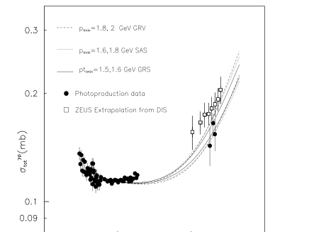
The two sets of data correspond respectively to photoproduction [22, 23] and to a recent extrapolation of the ‘nonzero-$Q^{2}$’ data [9]. In all these the parametrisation for the parton densities in the proton is GRV94 [24]. We have checked that the results are not affected if we use the GRV98 [25] parametrisation instead. As said before, the $b$ dependence can also be modelled by Fourier Transform of the intrinsic transverse momentum distribution of the partons. For the photonic partons this gives rise to a $b$ dependence which has the same analytical form as the form factor ansatz, but with a different value for the pole position [15] than with the form factor ansatz. All the curves correspond to using for the photon “form factor”

$${\cal F}(q^{2})={{k_{0}^{2}}\over{q^{2}+k_{0}^{2}}}$$ (10)

with $k_{0}=0.66\ GeV$ a value implied by the measurements by ZEUS, a value of $P_{had}=1/240$ and a soft cross-section $\sigma_{\gamma p}=constant+A/\sqrt{s}+B/s$.

With these values of the various parameters, one can obtain the photon-photon cross-sections. To do so, we use $P_{had}^{\gamma\gamma}=[P_{had}]^{2}$, $\sigma_{soft}^{\gamma\gamma}=2/3\sigma_{soft}^{\gamma p}$ and the same values for the $k_{0}$ scale in the photon form factor, same densities and $p_{tmin}$ values. The result is shown in Fig.3.

Figure 3: Comparison of photon-photon total cross-section data with EMM model

4 INELASTIC AND TOTAL PHOTON CROSS-SECTIONS IN THE EMM

We compare here two different applications of the eikonal minijet model for the photon cross-sections into hadrons, the total vs. inelastic mode. Namely, curves are obtained by fixing the parameters as described in the previous section, but using a fit to the photoproduction data considered as an inelastic cross-section. This kind of comparison would correspond to a situation such that the data did not include any of the so-called elastic part, namely vector meson production. The latter evaluation depending upon the model used for diffractive production, fitting the curve with

$$\sigma^{inel}=P_{had}\int d^{2}{\vec{b}}[1-e^{-n(b,s)}]$$ (11)

and then extrapolating to $\gamma\gamma$, again with the inelastic formulation, may provide an interpolation for the actual data for photon-photon between different models for the diffractive part. Proceeding as described, we obtain a slightly different set of parameters than the ones described in the previous section, including a value for $P_{had}\approx 1/200$ and a curve for photon -photon which lies higher than the previous one, with a more moderate rise.

Figure 4: Comparison of photon-photon total and inelastic cross-section predictions from the EMM.

The results are shown in Fig. 4. As first noticed in [12], the total EMM prediction is more in agreement with the L3 data (as extrapolated with Phojet), whereas the inelastic formulation follows better the trend of the OPAL data. To illustrate the dependence of the EMM predictions upon the scale parameter $k_{0}$, the inelastic formulation is shown with two curves, the lower of which is obtained with $k_{0}=1\ GeV$ value.

5 QCD MODEL FOR THE OVERLAP FUNCTION A(b)

In this last section we present some work in progress concerning a soft gluon summation model for the overlap function $A(b)$, which should hopefully reduce some of the arbitrariness of the mini-jet model, namely the dependence upon the impact parameter space distribution. In the previous section, the average number of hard collisions was given as

$$n_{hard}(b,s)=A(b)\sigma_{jet}(s,p_{tmin})/P_{had}$$ (12)

where $A(b)$ can be considered as the average number of scattering centers per unit area and, as mentioned, is obtained by convoluting the electromagnetic form factor of particles $a$ and $b$. The philosophy underlying this assumption is that not only matter distribution in the hadron follows the charge distribution, but also the quantochromodynamic field, the gluons, does. While this is certainly plausible, it does not allow for an ab-initio description. The parton-model improved ansatze of [18] is that there is no exact factorization between the variables in the transverse and longitudinal momentum, and that each subprocess characterized by a final jet momentum $p_{t}$ be defined through an impact parameter value $b$ whose distribution is obtained as the Fourier transform of the initial transverse momentum of the colliding pair, which was initially assumed collinear with the proton. In this model, which includes NLO corrections to the leading order Born parton-parton processes, one has

$$A(b)={{e^{-h(b,s)}}\over{\int d^{2}{\vec{b}}\ e^{-h(b,s)}}}$$ (13)

where

$$e^{-h(b,s)}=\int{{d^{2}{\vec{K}}_{t}}\over{(2\pi)^{2}}}\Pi(K_{t})e^{-iK_{t}\cdot b}$$ (14)

and $\Pi(K_{t})$ is the transverse momentum distribution of initial state soft gluon emission in the process

$$q{\bar{q}}\rightarrow X+{\rm jet\;\;jet}$$ (15)

In LLA, the function $h(b,s)$ is calculated from QCD to be given by[18]

$$h(b,s)={{2c_{F}}\over{\pi}}\int_{0}^{M}{{dk_{\perp}}\over{k_{\perp}}}\alpha_{s}({{k^{2}_{\perp}}\over{\Lambda^{2}}})$$

$$\ \ \ \times\ln{{M+\sqrt{M^{2}-k_{\perp}^{2}}}\over{M-\sqrt{M^{2}-k_{\perp}^{2}}}}[1-J_{0}(k_{\perp}b)]$$ (16)

where $M\simeq M(s,p_{tmin})$ is the maximum energy allowed for gluon emission in a process characterized by a given $p_{tmin}$ at any given energy $\sqrt{s}$. Thus the Bloch-Nordsieck improved b-distribution function is energy dependent, since the function $h(b,s)$ depends upon the maximum energy allowed for single gluon emission by each colliding parton, and a rather lengthy and complicate integration may be involved.

Figure 5: Predictions from the EMM implemented by Bloch-Nordieck summation.

Such impact parameter distribution inserted into the eikonal formalism of the minijet model describes a picture of multiparton collisions, each one of which is dressed by soft gluons. While this model has been recently[18] shown to give interesting results for the case of proton-proton, and proton-antiproton, work is in progress to determine the effect of such distribution on photon-photon cross-sections. A preliminary result is shown in Fig.5.

6 Conclusion

We have presented various predictions for the total $\gamma\gamma$ cross-section into hadrons, some of them based on a straightforward extension of the proton total cross-sections, others which depend more strongly on the chosen parton densities in the photons at small x. We notice that the rise of the total photon-photon cross-section can be accounted for through the QCD mini-jet models. We also see that more work is still needed, both on the theoretical and the experimental side, before being able to make realistic descriptions.

7 Acknowledgments

We wish to thank Prof. Martin Block for useful discussions.

References

- [1] L3 Collaboration, Paper 519 submitted to ICHEP’98, Vancouver, July 1998, M. Acciari et al., Phys. Lett. B 408 (1997) 450.
- [2] L3 Collaboration,A. Csilling, these Proceedings.
- [3] OPAL Collaboration , F. Waeckerle, Multiparticle Dynamics 1997, Nucl. Phys. B, (Proc. Suppl), 71 (1999) 381, Eds. G. Capon, V. Khoze, G. Pancheri and A. Sansoni; Stefan Söldner-Rembold, hep-ex/9810011, To appear in the proceedings of the ICHEP’98, Vancouver, July 1998.
- [4] G. Abbiendi et al., hep-ex/9906039, CERN-EP-99-076, Submitted to EPJC.
- [5] Review of Particle Properties, 1996.
- [6] G. Schuler and T. Sjöstrand, Two Photon Physics : from Daphane to LEP 200 and Beyond, Paris, Feb. 1994, World Scientific, 1994, p.163, Eds. F. Kapusta and J. Parisi; Zeit. Physik C 73 (1997) 677.
- [7] A. Donnachie and P.V. Landshoff, Phys. Lett.B 296 (1992) 227.
- [8] F. Abe et al., CDF Collaboration, Phys. Rev. D50 (1995) 5550
- [9] B. Surrow, DESY-THESIS-1998-004. A. Bornheim, In the Proceedings of the LISHEP International School on High Energy Physics, Brazil, 1998, hep-ex/9806021.
- [10] S. J. Brodsky, T. Kinoshita and H. Terazawa, Phys. Rev. D 4(1971) 1532.
- [11] C. Bourelly, J. Soffer and T.T. Wu, hep-ph/9903438, March 22nd, 1999.
- [12] M. Block, E. Gregores, F. Halzen and G. Pancheri, Phys. Rev. D 58 (1998) 1750; hep-ph/9809403 to appear in Phys. Rev. D.
- [13] B. Badelek,J. Kwiecinski and A.M. Stasto, hep-ph/9903248, March 3rd, 1999.
- [14] T. Sjöstrand and M. van Zijl, Phys. Rev. D 36 (1987) 2019.
- [15] A. Corsetti, R.M. Godbole and G. Pancheri, Phys. Lett. B 435 (1998) 441.
- [16] D.Cline, F.Halzen and J. Luthe, Phys. Rev. Lett. 31 (1973) 491; T.Gaisser and F.Halzen, Phys. Rev. Lett. 54 (1985) 1754.
- [17] L. Durand and H. Pi, Phys. Rev. Lett. 58 (1987) 58. A. Capella, J. Kwiecinski, J. Tran Thanh, Phys. Rev. Lett. 58 (1987) 2015. M.M. Block, F. Halzen, B. Margolis, Phys. Rev. D 45 (1992) 839.
- [18] A. Corsetti, A. Grau, G. Pancheri and Y. N. Srivastava, Phys.Lett. B382 (1996) 282; A. Grau, G. Pancheri and Y.N. Srivastava, hep-ph/9905228, to be pubblished in PRD.
- [19] M. Glück, E. Reya and A. Vogt, Phys. Rev. D 46 (1992) 1973.
- [20] G. Schuler and T. Sjöstrand, Zeit. Physik C 68 (1995) 607; Phys. Lett. B 376 (1996) 193.
- [21] M. Glück, E. Reya and I. Schienbein, hep-ph/9903337.
- [22] ZEUS Collaboration, Phys. Lett. B 293 (1992), 465; Zeit. Phys. C 63 (1994) 391.
- [23] H1 Collaboration, Zeit. Phys. C69 (1995) 27.
- [24] M. Glück, E. Reya and A. Vogt, Zeit. Physik C 67 (1994) 433.
- [25] M. Glück, E. Reya and A. Vogt, Eur. Phys. Jou. C 5 (1998) 461.