More about on the short distance contribution to the $B_{c}\rightarrow B_{u}^{\ast}\gamma$ decay


T. M. Aliev   , M. SavcΔ±
Physics Department, Middle East Technical University
06531 Ankara, Turkey
e-mail: taliev@metu.edu.tre-mail: savci@metu.edu.tr

We calculate the transition form factor for the $B_{c}\rightarrow B_{u}^{\ast}\gamma$ decay taking into account only the short distance contribution, in framework of QCD sum rules method. We observe that the transition form factor predicted by the QCD sum rules method is approximately two times larger compared to the result predicted by the Isgur, Scora, Grinstein and Wise model.

1 Introduction

Flavor changing neutral current (FCNC) transitions constitute one of the most important research area in particle physics. In standard model (SM) these transitions take place only at one loop level. Therefore the study of the rare decays allows us to check the gauge structure of the SM and can provide valuable information for a more precise determination of the Cabibbo–Kobayashi–Maskawa matrix elements, leptonic decay constants, etc., which are poorly known today.

In the SM the FCNC transitions of the down–quark sector have relatively large branching ratio, due to the large mass of the top quark running in the loop and $b\rightarrow s$ transition has already been observed in experiments [1]. On the other hand, in up quark–sector of the SM these transitions are quite rare since in the loop down quark runs which has smaller mass compared to top quark mass. At present only the upper experimental bounds on the FCNC transitions of the up quark sector exist [2].

To probe the very rare $c\rightarrow u\gamma$ transition in SM, it was shown in [3] that the radiative beauty conserving $B_{c}\rightarrow B_{u}^{\ast}\gamma$ decay is very promising. It should be noted that $B_{c}$ meson has been observed by the CDF Collaboration at Fermilab [4]. This decay receives short and long distance contributions. The short distance contribution in $B_{c}\rightarrow B_{u}^{\ast}\gamma$ decay comes from FCNC $c\rightarrow u\gamma$ transition when $\bar{b}$ is a spectator quark. The long distance contributions to $B_{c}\rightarrow B_{u}^{\ast}\gamma$ decay can be grouped into two classes:

I) Vector meson dominance contribution which corresponds the processes $c\rightarrow uq_{i}\bar{q}_{i}$, is followed by the conversion of $q_{i}\bar{q}_{i}$ pair to photon while $\bar{b}$ is spectator again, which is similar to the short distance contribution case.

II) Annihilation contribution mechanism, which corresponds to the annihilation process $c\bar{b}\rightarrow u\bar{b}$ where photon is attached to any quark line.

The short and long distance effects to this decay are calculated in framework of the Isgur, Scora, Grinstein and Wise (ISGW) model [5] and it is found that both contributions are comparable to each other which allows, in principle, probing $c\rightarrow u\gamma$ transition. It is found that the branching ratio is of the order of $\sim 10^{-8}$ and can be detectable at future LHC. This result is quite interesting and is the first example where short and long distance effects for the $c\rightarrow u\gamma$ transition are comparable, contrary to the corresponding $D$ meson decays for which long distance contribution is dominant [6]–[8]. Therefore this observation opens the way to extract the short distance $c\rightarrow u\gamma$ contribution from the experiment. For this reason, in order to check this principal result it is necessary to perform these calculations still in another framework.

In the present letter, we calculate the form factor for the $B_{c}\rightarrow B_{u}^{\ast}\gamma$ decay due to the short distance contribution only, in frame work of the QCD sum rules. It is observed that the value of the form factor calculated in the QCD sum rules is approximately two times larger compared to the one predicted by the ISGW model. As a result, it seems that in the $B_{c}\rightarrow B_{u}^{\ast}\gamma$ decay case, the short and long distance contributions are of the same order. This circumstance opens the way for a real possibility of probing rare $c\rightarrow u\gamma$ transition via $B_{c}\rightarrow B_{u}^{\ast}\gamma$ decay.

As has been noted already, we restrict ourselves only to the short distance contribution to the $B_{c}\rightarrow B_{u}^{\ast}\gamma$ decay. The short distance contribution to the $B_{c}\rightarrow B_{u}^{\ast}\gamma$ decay is obtained from $c\rightarrow u\gamma$ transition, where $\bar{b}$ quark is a spectator. The effective Hamiltonian for the $c\rightarrow u\gamma$ transition is given as

β„‹e​f​f=βˆ’GF2​e4​π2​Vc​s​Vu​sβˆ—β€‹C7​(ΞΌ)​u¯​σμ​ν​[mc​1+Ξ³52+mu​1βˆ’Ξ³52]​c​ℱμ​ν,subscriptℋ𝑒𝑓𝑓subscript𝐺𝐹2𝑒4superscriptπœ‹2subscript𝑉𝑐𝑠superscriptsubscriptπ‘‰π‘’π‘ βˆ—subscript𝐢7πœ‡Β―π‘’subscriptπœŽπœ‡πœˆdelimited-[]subscriptπ‘šπ‘1subscript𝛾52subscriptπ‘šπ‘’1subscript𝛾52𝑐superscriptβ„±πœ‡πœˆ\displaystyle{\cal H}_{eff}=-\frac{G_{F}}{\sqrt{2}}\frac{e}{4\pi^{2}}V_{cs}V_{us}^{\ast}C_{7}(\mu)\bar{u}\sigma_{\mu\nu}\left[m_{c}\frac{1+\gamma_{5}}{2}+m_{u}\frac{1-\gamma_{5}}{2}\right]c\,{\cal F}^{\mu\nu}~{}, (1)

where $V_{ij}$ correspond to the CKM matrix elements, and ${\cal F}_{\mu\nu}$ is the electromagnetic field strength tensor. The appropriate scale for $C_{7}(\mu)$ is $\mu=m_{c}$ since $\bar{b}$ quark is the spectator for the short distance contribution in the $B_{c}\rightarrow B_{u}^{\ast}\gamma$ decay. In further calculations we will take the mass of the up quark to be zero.

The two loop QCD corrections to the $c\rightarrow u\gamma$ transition was calculated in [9] whose prediction is $C_{7}(m_{c})=-0.0068-0.02i$ and this result is scheme independent. In order to calculate the amplitude for the $B_{c}\rightarrow B_{u}^{\ast}\gamma$ decay, the matrix elements

$\displaystyle\left<B_{u}^{\ast}\left|\bar{u}\sigma_{\mu\nu}(1\pm\gamma_{5})q^{\nu}\right|B_{c}\right>~{},$

need to be calculated at $q^{2}=0$, where $q$ is the photon four–momentum. These matrix elements can be written in terms of two gauge invariant form factors $F_{1}(0)$ and $F_{2}(0)$ as follows:

$\displaystyle\left<B_{u}^{\ast}(p^{\prime},\varepsilon^{\prime})\left|\bar{u}i\sigma_{\mu\nu}q^{\nu}c\right|B_{c}(p)\right>$ $\displaystyle=$ $\displaystyle i\epsilon_{\mu\alpha\beta\rho}\varepsilon^{\prime\alpha}p^{\prime\beta}q^{\rho}F_{1}(0)~{},$
$\displaystyle\left<B_{u}^{\ast}(p^{\prime},\varepsilon^{\prime})\left|\bar{u}i\sigma_{\mu\nu}q^{\nu}\gamma_{5}c\right|B_{c}(p)\right>$ $\displaystyle=$ $\displaystyle\left[\left(m_{B_{c}}^{2}-m_{B_{u}^{\ast}}^{2}\right)\varepsilon_{\mu}^{\prime}-\left(\varepsilon^{\prime}q\right)\left(p+p^{\prime}\right)_{\mu}\right]F_{2}(0)~{}.$ (2)

Using the relation

$\displaystyle\sigma_{\mu\nu}\gamma_{5}=-\frac{i}{2}\epsilon_{\mu\nu\alpha\beta}\sigma^{\alpha\beta}~{},$ (3)

one can easily show that $F_{2}(0)=F_{1}(0)/2$. Therefore in order to calculate the short distance part of the $B_{c}\rightarrow B_{u}^{\ast}\gamma$ decay it is enough to calculate $F_{1}(0)$ or $F_{2}(0)$, for which we will employ the three–point QCD sum rules [10, 11]. For the evolution of the form factor $F_{1}(0)$ in framework of the QCD sum rules, we consider the following three–point function

Πμ​α=βˆ’βˆ«d4​x​d4​y​ei​(p​xβˆ’p′​y)β€‹βŸ¨0|T​{b¯​(y)​γα​u​(y)​u¯​(0)​i​σμ​ν​qν​c​(0)​c¯​(x)​i​γ5​b​(x)}|0⟩,subscriptΞ πœ‡π›Όsuperscript𝑑4π‘₯superscript𝑑4𝑦superscript𝑒𝑖𝑝π‘₯superscript𝑝′𝑦quantum-operator-product0T¯𝑏𝑦subscript𝛾𝛼𝑒𝑦¯𝑒0𝑖subscriptπœŽπœ‡πœˆsuperscriptπ‘žπœˆπ‘0¯𝑐π‘₯𝑖subscript𝛾5𝑏π‘₯0\displaystyle\Pi_{\mu\alpha}=-\int d^{4}xd^{4}ye^{i(px-p^{\prime}y)}\left<0\left|\mbox{\rm T}\Big{\{}\bar{b}(y)\gamma_{\alpha}u(y)\bar{u}(0)i\sigma_{\mu\nu}q^{\nu}c(0)\bar{c}(x)i\gamma_{5}b(x)\Big{\}}\right|0\right>~{}, (4)

where $\bar{b}\gamma_{\alpha}u$ and $\bar{c}i\gamma_{5}b$ are the interpolating currents for states with the $B_{u}^{\ast}$ and $B_{c}$ mesons, respectively. The Lorentz structure in the correlator (4) can be written as

Πμ​ν=i​ϡμ​ν​α​β​pα​p′⁣β​Π,subscriptΞ πœ‡πœˆπ‘–subscriptitalic-Ο΅πœ‡πœˆπ›Όπ›½superscript𝑝𝛼superscript𝑝′𝛽Π\displaystyle\Pi_{\mu\nu}=i\epsilon_{\mu\nu\alpha\beta}p^{\alpha}p^{\prime\beta}\,\Pi~{}, (5)

where scalar amplitude Ξ Ξ \Pi is the function of the kinematical invariants, i.e., Ξ =Π​(p2,p′⁣2)Ξ Ξ superscript𝑝2superscript𝑝′2\Pi=\Pi(p^{2},p^{\prime 2}).

In accordance with the usual QCD sum rules philosophy, the theoretical part of the three–point correlator can be calculated by employing the operator product expansion (OPE) for the T–ordered product of currents in (4). The values of the heavy quark condensates are related to the vacuum expectation values of the gluon operators. For example

⟨Q​Q¯⟩=βˆ’112​mQ​αsΟ€β€‹βŸ¨G2βŸ©βˆ’1360​mQ3​αsΟ€β€‹βŸ¨G2βŸ©β€‹β‹―,delimited-βŸ¨βŸ©π‘„Β―π‘„112subscriptπ‘šπ‘„subscriptπ›Όπ‘ πœ‹delimited-⟨⟩superscript𝐺21360superscriptsubscriptπ‘šπ‘„3subscriptπ›Όπ‘ πœ‹delimited-⟨⟩superscript𝐺2β‹―\displaystyle\left<Q\bar{Q}\right>=-\frac{1}{12m_{Q}}\frac{\alpha_{s}}{\pi}\left<G^{2}\right>-\frac{1}{360m_{Q}^{3}}\frac{\alpha_{s}}{\pi}\left<G^{2}\right>\cdots~{}, (6)

where $Q$ is the heavy quark and the heavy quark condensate contributions are suppressed by inverse of the heavy quark mass. for this reason we safely omit them in our calculations.

It should be stressed that the light quark condensate does not give any contribution to the above–mentioned decay after double Borel transformation. Therefore the only non–perturbative contribution to the $B_{c}\rightarrow B_{u}^{\ast}\gamma$ decay comes from gluon condensate.

So, in the lowest order of perturbation theory, the three–point function is given by the bare quark loop and by gluon condensate contribution. The contribution to the three–point function from the bare loop can be obtained using the double dispersion representation in $p^{2}$ and $p^{\prime 2}$

Ξ p​e​r​(p2,p′⁣2)=βˆ’14​π2β€‹βˆ«Οp​e​r​(p2,p′⁣2)(sβˆ’p2)​(sβ€²βˆ’p′⁣2)​𝑑s​𝑑sβ€²+sub. terms.superscriptΞ π‘π‘’π‘Ÿsuperscript𝑝2superscript𝑝′214superscriptπœ‹2superscriptπœŒπ‘π‘’π‘Ÿsuperscript𝑝2superscript𝑝′2𝑠superscript𝑝2superscript𝑠′superscript𝑝′2differential-d𝑠differential-dsuperscript𝑠′sub. terms\displaystyle\Pi^{per}(p^{2},p^{\prime 2})=-\frac{1}{4\pi^{2}}\int\displaystyle{\frac{\rho^{per}(p^{2},p^{\prime 2})}{(s-p^{2})(s^{\prime}-p^{\prime 2})}}dsds^{\prime}+\mbox{\rm sub. terms}~{}. (7)

The spectral density $\rho^{per}(p^{2},p^{\prime 2})$ can be calculated using the Cutkovsky rule, i.e., by replacing propagators with delta functions:

$\displaystyle\left(k^{2}-m_{i}^{2}\right)^{-1}\rightarrow-2\pi i\delta(k^{2}-m_{i}^{2})~{}.$

After standard calculations for the spectral density we get

ρp​e​r​(s,sβ€²)=4​Nc​{mc​mb​[A1+A2+ℐ0]βˆ’mc2​A1βˆ’2​A},superscriptπœŒπ‘π‘’π‘Ÿπ‘ superscript𝑠′4subscript𝑁𝑐subscriptπ‘šπ‘subscriptπ‘šπ‘delimited-[]subscript𝐴1subscript𝐴2subscriptℐ0superscriptsubscriptπ‘šπ‘2subscript𝐴12𝐴\displaystyle\rho^{per}(s,s^{\prime})=4N_{c}\Big{\{}m_{c}m_{b}\left[A_{1}+A_{2}+{\cal I}_{0}\right]-m_{c}^{2}A_{1}-2A\Big{\}}~{}, (9)

where

$\displaystyle A_{1}$ $\displaystyle=$ $\displaystyle\frac{2{\cal I}_{0}}{(s-s^{\prime})^{2}}\Bigg{[}s^{\prime}(s+m_{b}^{2}-m_{c}^{2})-\frac{1}{2}(s+s^{\prime})(s^{\prime}+m_{b}^{2})\Bigg{]}~{},$
$\displaystyle A_{2}$ $\displaystyle=$ $\displaystyle\frac{2{\cal I}_{0}}{(s-s^{\prime})^{2}}\Bigg{[}\frac{1}{2}(s+s^{\prime})(m_{c}^{2}-m_{b}^{2}-s)+s(s^{\prime}+m_{b}^{2})\Bigg{]}~{},$
$\displaystyle A$ $\displaystyle=$ $\displaystyle{\cal I}_{0}\,\,\frac{m_{c}^{2}\left[m_{c}^{2}s^{\prime}+(m_{b}^{2}-s^{\prime})(s-s^{\prime})\right]}{2(s-s^{\prime})^{2}}~{},$
$\displaystyle{\cal I}_{0}$ $\displaystyle=$ $\displaystyle-\frac{1}{4(s-s^{\prime})}~{},$ (10)

and $N_{c}$ is the color number.

The region of integration over $s$ and $s^{\prime}$ is determined by the following inequalities

$\displaystyle m_{b}^{2}\leq s^{\prime}\leq s_{0}^{\prime}~{},$
$\displaystyle s^{\prime}-\frac{s^{\prime}m_{c}^{2}}{m_{b}^{2}-s^{\prime}}\leq s\leq s_{0}~{}.$ (11)

Note that we have neglected π’ͺ​(Ξ±s/Ο€)π’ͺsubscriptπ›Όπ‘ πœ‹{\cal O}(\alpha_{s}/\pi) hard gluon corrections to the triangle diagram, as they are not available yet. However, we expect their contribution to be about $\sim 10\%$, so that if the accuracy of the QCD sum rules is taken into account, these corrections would not change the results drastically.

From our result on spectral density we can get the spectral density for $B\rightarrow K^{\ast}\gamma$ decay (when msβ†’0β†’subscriptπ‘šπ‘ 0m_{s}\rightarrow 0) if we formally make the replacements $m_{b}\rightarrow 0$ and $m_{c}\rightarrow m_{b}$ in Eqs. (9) and (10). Indeed, our results coincide with the results of [12] for $B\rightarrow K^{\ast}\gamma$ decay, after the above–mentioned substitutions are performed. The gluon condensate contribution to three–point correlator (4) is given by diagrams depicted in Fig. (1). The calculations of these diagrams were carried out in the Fock–Schwinger fixed point gauge [13, 14, 15]; $x^{\mu}A_{\mu}(x)=0$. For calculation of the gluon condensate contributions, we have used the Schwinger representation for the Euclidean propagators, i.e.,

$\displaystyle\frac{1}{\Big{[}k^{2}+m^{2}\Big{]}^{a}}=\frac{1}{\Gamma(a)}\int_{0}^{\infty}d\alpha\,\alpha^{n-1}e^{-\alpha(k^{2}+m^{2})}~{},$ (12)

which is very suitable for applying the Borel transformation, since

$\displaystyle\hat{B}_{p^{2}}(M^{2})\,e^{-\alpha p^{2}}=\delta(1-\alpha M^{2})~{}.$ (13)

The analytical expression for the Wilson coefficient of the gluon condensate operator $C_{G^{2}}$ is quite lengthy and for this reason it is presented in the appendix.

It should be noted that Borel transformed Wilson coefficient of the gluon condensate contribution in the three point sum rules with arbitrary mass, which appears in the study of the form factors for the vector and axial vector current transitions of the semileptonic $B_{c}\rightarrow J/\psi\ell\nu$ decay, was investigated in detail in [16].

We now turn our attention to the computation of the physical part of the sum rules. Assuming that the spectral density is well convergent, the physical spectral density is saturated by the lowest lying hadronic states plus a continuum starting at some effective thresholds $s_{0},~{}s_{0}^{\prime}$

ρμ​αp​h​y​(s,sβ€²)=ρμ​αr​e​s​(s,sβ€²)+θ​(sβˆ’s0)​θ​(sβ€²βˆ’s0β€²)​ρμ​αc​o​n​t​(s,sβ€²),subscriptsuperscriptπœŒπ‘β„Žπ‘¦πœ‡π›Όπ‘ superscript𝑠′subscriptsuperscriptπœŒπ‘Ÿπ‘’π‘ πœ‡π›Όπ‘ superscriptπ‘ β€²πœƒπ‘ subscript𝑠0πœƒsuperscript𝑠′superscriptsubscript𝑠0β€²subscriptsuperscriptπœŒπ‘π‘œπ‘›π‘‘πœ‡π›Όπ‘ superscript𝑠′\displaystyle\rho^{phy}_{\mu\alpha}(s,s^{\prime})=\rho^{res}_{\mu\alpha}(s,s^{\prime})+\theta(s-s_{0})\theta(s^{\prime}-s_{0}^{\prime})\rho^{cont}_{\mu\alpha}(s,s^{\prime})~{}, (14)

where

ρμ​αr​e​ssubscriptsuperscriptπœŒπ‘Ÿπ‘’π‘ πœ‡π›Ό\displaystyle\rho^{res}_{\mu\alpha} $\displaystyle=$ $\displaystyle\left<0\left|\bar{c}i\gamma_{5}b\right|B_{c}\right>\left<B_{c}\left|\bar{u}i\sigma_{\mu\nu}q^{\nu}c\right|B_{u}^{\ast}\right>\left<B_{u}^{\ast}\left|\bar{b}\gamma_{\alpha}u\right|0\right>$ (15)
$\displaystyle\times$ $\displaystyle(2\pi)^{2}\delta(s-M_{B_{c}}^{2})\delta(s^{\prime}-M_{B_{u}^{\ast}}^{2})~{},$

and $\rho^{cont}$ corresponds to the continuum contribution. The matrix elements in (15) are defined in the following way:

$\displaystyle\left<0\left|\bar{c}i\gamma_{5}b\right|B_{c}\right>$ $\displaystyle=$ $\displaystyle\frac{f_{B_{c}}m_{B_{c}}^{2}}{m_{b}+m_{c}}~{},$
$\displaystyle\left<B_{u}^{\ast}\left|\bar{b}\gamma_{\alpha}u\right|0\right>$ $\displaystyle=$ $\displaystyle f_{B_{u}^{\ast}}m_{B_{u}^{\ast}}\varepsilon_{\alpha}^{\ast}~{}.$

Selecting the structure $i\epsilon_{\mu\nu\alpha\beta}p^{\alpha}p^{\prime\beta}$ for ρr​e​ssuperscriptπœŒπ‘Ÿπ‘’π‘ \rho^{res}, we have

ρr​e​s=fBc​mBc2mb+mc​fBuβˆ—β€‹mBuβˆ—β€‹F1​(0)​(2​π)2​δ​(sβˆ’MBc2)​δ​(sβ€²βˆ’MBuβˆ—2).superscriptπœŒπ‘Ÿπ‘’π‘ subscript𝑓subscript𝐡𝑐superscriptsubscriptπ‘šsubscript𝐡𝑐2subscriptπ‘šπ‘subscriptπ‘šπ‘subscript𝑓superscriptsubscriptπ΅π‘’βˆ—subscriptπ‘šsuperscriptsubscriptπ΅π‘’βˆ—subscript𝐹10superscript2πœ‹2𝛿𝑠superscriptsubscript𝑀subscript𝐡𝑐2𝛿superscript𝑠′superscriptsubscript𝑀superscriptsubscriptπ΅π‘’βˆ—2\displaystyle\rho^{res}=\frac{f_{B_{c}}m_{B_{c}}^{2}}{m_{b}+m_{c}}f_{B_{u}^{\ast}}m_{B_{u}^{\ast}}F_{1}(0)(2\pi)^{2}\delta(s-M_{B_{c}}^{2})\delta(s^{\prime}-M_{B_{u}^{\ast}}^{2})~{}.

The continuum contribution is modeled as a perturbative contribution starting from thresholds $s_{0}$ and $s_{0}^{\prime}$. Equating (15) to the theoretical part contribution (7) and performing double Borel transformations with respect to the parameters $p^{2}$ and $p^{\prime 2}$, we finally get the following sum rule for the transition form factor:

$\displaystyle F_{1}(0)$ $\displaystyle=$ $\displaystyle\frac{(m_{b}+m_{c})}{f_{B_{u}^{\ast}}m_{B_{u}^{\ast}}f_{B_{c}}m_{B_{c}}^{2}}e^{m_{B_{c}}^{2}/M_{1}^{2}}e^{m_{B_{u}^{\ast}}^{2}/M_{2}^{2}}$ (16)
$\displaystyle\times$ {βˆ’14​π2β€‹βˆ«π‘‘s​𝑑s′​ρ​(s,sβ€²)​eβˆ’s/M12​eβˆ’sβ€²/M22+M12​M22β€‹βŸ¨Ξ±sπ​G2βŸ©β€‹CG2},14superscriptπœ‹2differential-d𝑠differential-dsuperscriptπ‘ β€²πœŒπ‘ superscript𝑠′superscript𝑒𝑠superscriptsubscript𝑀12superscript𝑒superscript𝑠′superscriptsubscript𝑀22superscriptsubscript𝑀12superscriptsubscript𝑀22delimited-⟨⟩subscriptπ›Όπ‘ πœ‹superscript𝐺2subscript𝐢superscript𝐺2\displaystyle\Bigg{\{}-\frac{1}{4\pi^{2}}\int dsds^{\prime}\rho(s,s^{\prime})e^{-s/M_{1}^{2}}e^{-s^{\prime}/M_{2}^{2}}+M_{1}^{2}M_{2}^{2}\langle\frac{\alpha_{s}}{\pi}G^{2}\rangle C_{G^{2}}\Bigg{\}}~{},

where $C_{G^{2}}$ is the Wilson coefficient of the gluon condensate contribution. This expression is the final result for the transition form factor evaluated at $q^{2}=0$.

For the numerical analysis we have used the following values of the input parameters that enter into sum rules (16): $f_{B_{c}}=385~{}MeV$ [17], $f_{B_{u}^{\ast}}=160~{}MeV$ [18], $m_{c}=1.4~{}GeV$, $\langle\alpha_{s}G^{2}/\pi\rangle=0.012~{}GeV^{4}$ [10], $s_{0}=50~{}GeV^{2}$ and $s_{0}^{\prime}=35~{}GeV^{2}$. As is obvious, Eq. (16) involves two independent Borel parameters $M_{1}^{2},~{}M_{2}^{2}$, and then the main problem is finding the region where the dependence of these parameters is weak and at the same time power corrections and the continuum remains under control.

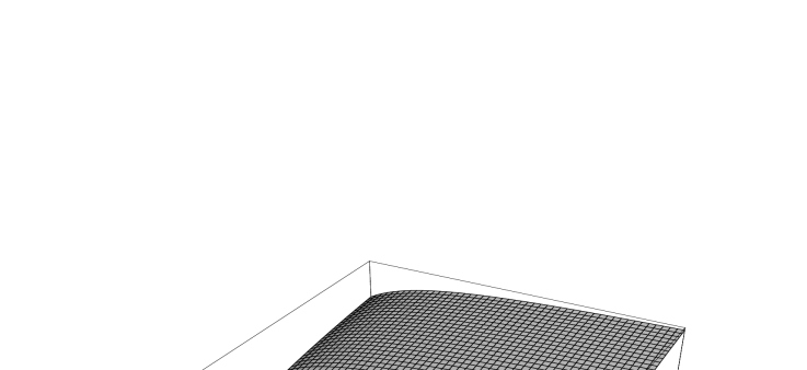
In Fig. (2) we present the dependence of the transition form factor $F_{1}(0)$ on $M_{1}^{2}$ and $M_{2}^{2}$. Numerical calculations show that the best stability for the form factor $F_{1}(0)$ is achieved for $15~{}GeV^{2}\leq M_{1}^{2}\leq 20~{}GeV^{2}$ and $8~{}GeV^{2}\leq M_{2}^{2}\leq 12~{}GeV^{2}$. Our final result for the form factor is

$\displaystyle F_{1}(0)=(0.9\pm 0.1)~{}.$

For a comparison, we note that the IGSW model’s prediction for this transition form factor is $F_{1}(0)=0.48$ [3]. Therefore the branching ratio in our case is approximately four times larger compared to that predicted in [3]. It should be stressed again that in the present work only the short distance contribution to the $B_{c}\rightarrow B_{u}^{\ast}\gamma$ decay is considered.

Using this result we observe that the short distance contribution to the branching ratio is of the order of $\sim 2\times 10^{-8}$, which can be quite detectable at future LHC. Moreover our result show that the short distance contribution in our approach is comparable or larger than the long distance contribution calculated in [3]

$\displaystyle{\cal B}\left(B_{c}\rightarrow B_{u}^{\ast}\gamma\right)=\left(7.5^{\displaystyle{+7.7}}_{\displaystyle{-4.3}}\right)\times 10^{-9},$

and our result proves that there is indeed real possibility for probing the $c\rightarrow u\gamma$ decay via the beauty conserving $B_{c}\rightarrow B_{u}^{\ast}\gamma$ decay.

As the final remark we would like to note that the approach presented in this work is applicable for calculating the short distance contributions to the branching ratio of the $B_{s}\rightarrow B_{d}^{\ast}\gamma$ and Bcβ†’Dsβˆ—β€‹Ξ³β†’subscript𝐡𝑐superscriptsubscriptπ·π‘ βˆ—π›ΎB_{c}\rightarrow D_{s}^{\ast}\gamma decays.

Appendix : The gluon condensate contribution

In this section we will present the explicit expressions for the Wilson coefficients $C_{G^{2}}$ for each diagram, after the Borel transformation with respect to $p^{2}$ and $p^{\prime 2}$, which are presented in Fig. (1).

 
$\displaystyle(C_{G^{2}})_{1}=96m_{c}\Big{\{}\Big{[}m_{b}\Big{(}I_{0}[1,3,1]+m_{c}^{2}I_{0}[1,4,1]+I_{1}[1,3,1]+m_{c}^{2}I_{1}[1,4,1]$
$\displaystyle{{}+I_{2}[1,3,1]-m_{c}^{2}I_{2}[1,4,1]\Big{)}\Big{]}+m_{c}\Big{(}I_{1}[1,3,1]+m_{c}^{2}I_{1}[1,4,1]+2I_{3}[1,4,1]\Big{)}\Big{\}}~{},}$
 
(A.1)

 
$\displaystyle(C_{G^{2}})_{2}=16\Big{\{}2I_{0}[1,1,2]+2m_{c}m_{b}I_{0}[1,1,3]+2I_{0}[2,1,1]+3m_{c}m_{b}I_{0}[2,1,2]$
$\displaystyle{{}+4m_{b}^{2}I_{0}[2,1,2]+4m_{c}m_{b}^{3}I_{0}[2,1,3]+2m_{c}m_{b}I_{0}[3,1,1]+2m_{b}^{2}I_{0}[3,1,1]}$
$\displaystyle{{}+6m_{c}m_{b}^{3}I_{0}[3,1,2]+2m_{b}^{4}I_{0}[3,1,2]+2m_{c}m_{b}^{5}I_{0}[3,1,3]+2I_{1}[1,1,2]}$
$\displaystyle{{}-2m_{c}^{2}I_{1}[1,1,3]+2m_{c}m_{b}I_{1}[1,1,3]+2I_{1}[2,1,1]-m_{c}^{2}I_{1}[2,1,2]}$
$\displaystyle{{}+m_{c}m_{b}I_{1}[2,1,2]+4m_{b}^{2}I_{1}[2,1,2]-4m_{c}^{2}m_{b}^{2}I_{1}[2,1,3]+4m_{c}m_{b}^{3}I_{1}[2,1,3]}$
$\displaystyle{{}-2m_{c}^{2}I_{1}[3,1,1]+2m_{b}^{2}I_{1}[3,1,1]-6m_{c}^{2}m_{b}^{2}I_{1}[3,1,2]+4m_{c}m_{b}^{3}I_{1}[3,1,2]}$
$\displaystyle{{}+2m_{b}^{4}I_{1}[3,1,2]-2m_{c}^{2}m_{b}^{4}I_{1}[3,1,3]+2m_{c}m_{b}^{5}I_{1}[3,1,3]+2m_{c}m_{b}I_{2}[1,1,3]}$
$\displaystyle{{}+I_{2}[2,1,1]+m_{c}m_{b}I_{2}[2,1,2]+4m_{c}m_{b}^{3}I_{2}[2,1,3]-4m_{b}^{2}I_{2}[3,1,1]}$
$\displaystyle{{}+4m_{c}m_{b}^{3}I_{2}[3,1,2]+2m_{c}m_{b}^{5}I_{2}[3,1,3]-4I_{3}[1,1,3]-4I_{3}[2,1,2]}$
$\displaystyle{{}-8m_{b}^{2}I_{3}[2,1,3]-8I_{3}[3,1,1]-16m_{b}^{2}I_{3}[3,1,2]-4m_{b}^{4}I_{3}[3,1,3]\Big{\}}}$
$\displaystyle{{}-32M_{2}^{2}\frac{d}{dM_{2}^{2}}\Big{\{}M_{2}^{2}\Big{[}I_{0}[2,1,2]+2m_{c}m_{b}I_{0}[2,1,3]+2m_{c}m_{b}I_{0}[3,1,2]}$
$\displaystyle{{}+m_{b}^{2}I_{0}[3,1,2]+2m_{c}m_{b}^{3}I_{0}[3,1,3]+I_{1}[2,1,2]-2m_{c}^{2}I_{1}[2,1,3]+2m_{c}m_{b}I_{1}[2,1,3]}$
$\displaystyle{{}-2m_{c}^{2}I_{1}[3,1,2]+m_{c}m_{b}I_{1}[3,1,2]+m_{b}^{2}I_{1}[3,1,2]-2m_{c}^{2}m_{b}^{2}I_{1}[3,1,3]}$
$\displaystyle{{}+2m_{c}m_{b}^{3}I_{1}[3,1,3]-I_{2}[2,1,2]+2m_{c}m_{b}I_{2}[2,1,3]-2I_{2}[3,1,1]}$
$\displaystyle{{}+m_{c}m_{b}I_{2}[3,1,2]-m_{b}^{2}I_{2}[3,1,2]+2m_{c}m_{b}^{3}I_{2}[3,1,3]-4I_{3}[2,1,3]}$
$\displaystyle{{}-6I_{3}[3,1,2]-4m_{b}^{2}I_{3}[3,1,3]\Big{]}\Big{\}}}$
$\displaystyle{{}-32M_{2}^{4}\left(\frac{d^{2}}{dM_{2}^{2}}\right)^{2}\Big{\{}M_{2}^{4}\Big{[}m_{c}^{2}I_{1}[3,1,3]+2I_{2}[3,1,2]-m_{c}m_{b}\Big{(}I_{0}[3,1,3]+I_{1}[3,1,3]}$
$\displaystyle{{}+I_{2}[3,1,3]\Big{)}+2I_{3}[3,1,3]\Big{]}\Big{\}}~{},}$
 
(A.2)

 
$\displaystyle(C_{G^{2}})_{3}=96m_{b}\Big{\{}-\Big{(}m_{c}^{2}m_{b}I_{1}[4,1,1]\Big{)}+m_{c}\Big{(}I_{0}[3,1,1]+m_{b}^{2}I_{0}[4,1,1]$
$\displaystyle{{}+I_{1}[3,1,1]+m_{b}^{2}I_{1}[4,1,1]+I_{2}[3,1,1]+m_{b}^{2}I_{2}[4,1,1]\Big{)}-2m_{b}I_{3}[4,1,1]\Big{\}}~{},}$
 
(A.3)

 
$\displaystyle(C_{G^{2}})_{4}=-32m_{c}m_{b}\Big{\{}I_{0}[2,1,2]+I_{0}[3,1,1]+m_{b}^{2}I_{0}[3,1,2]+I_{1}[2,1,2]+m_{b}^{2}I_{1}[3,1,2]$
$\displaystyle{{}+I_{2}[2,1,2]+m_{b}^{2}I_{2}[3,1,2]-4I_{3}[3,1,2]-M_{2}^{2}\frac{d}{dM^{2}}\Big{[}M_{2}^{2}\Big{(}I_{0}[3,1,2]+I_{1}[3,1,2]}$
$\displaystyle{{}+I_{2}[3,1,2]\Big{)}\Big{]}\Big{\}}+16\Big{\{}m_{c}^{2}I_{1}[2,1,2]+I_{2}[2,1,1]-m_{c}m_{b}\Big{(}I_{0}[2,1,2]+I_{1}[2,1,2]}$
$\displaystyle{{}+I_{2}[2,1,2]\Big{)}+4I_{3}[2,1,2]\Big{\}}~{},}$
 
(A.4)

 
$\displaystyle(C_{G^{2}})_{5}=16\Big{\{}2I_{0}[1,1,2]+I_{0}[1,2,1]+2m_{c}^{2}I_{0}[1,2,2]+m_{c}m_{b}I_{0}[1,2,2]$
$\displaystyle{{}+m_{b}^{2}I_{0}[2,1,2]+m_{c}m_{b}I_{0}[2,2,1]+m_{b}^{2}I_{0}[2,2,1]+m_{c}^{2}m_{b}^{2}I_{0}[2,2,2]}$
$\displaystyle{{}+m_{c}m_{b}^{3}I_{0}[2,2,2]+I_{1}[1,1,2]+I_{1}[1,2,1]+m_{c}^{2}I_{1}[1,2,2]}$
$\displaystyle{{}+m_{c}m_{b}I_{1}[1,2,2]-I_{1}[2,1,1]-2m_{c}m_{b}I_{1}[2,1,2]-m_{c}^{2}I_{1}[2,2,1]}$
$\displaystyle{{}+m_{b}^{2}I_{1}[2,2,1]-2m_{c}^{3}m_{b}I_{1}[2,2,2]+m_{c}m_{b}^{3}I_{1}[2,2,2]+I_{2}[1,1,2]}$
$\displaystyle{{}+I_{2}[1,2,1]+m_{c}^{2}I_{2}[1,2,2]+m_{c}m_{b}I_{2}[1,2,2]-2m_{c}m_{b}I_{2}[2,2,1]}$
$\displaystyle{{}+m_{b}^{2}I_{2}[2,2,1]+m_{c}m_{b}^{3}I_{2}[2,2,2]-2I_{3}[2,1,2]-4I_{3}[2,2,1]}$
$\displaystyle{{}-2m_{c}^{2}I_{3}[2,2,2]-4m_{c}m_{b}I_{3}[2,2,2]\Big{\}}}$
$\displaystyle{{}-16M_{1}^{2}\frac{d}{dM_{1}^{2}}\Big{\{}M_{1}^{2}\Big{[}I_{2}[2,2,1]+2I_{3}[2,2,2]\Big{]}\Big{\}}}$
$\displaystyle{{}+16M_{2}^{2}\frac{d}{dM_{2}^{2}}\Big{\{}M_{2}^{2}\Big{[}-m_{c}m_{b}I_{0}[2,2,2]+I_{1}[2,1,2]+m_{c}^{2}I_{1}[2,2,2]-m_{c}m_{b}I_{1}[2,2,2]}$
$\displaystyle{{}+I_{2}[2,1,2]+I_{2}[2,2,1]+m_{c}^{2}I_{2}[2,2,2]-m_{c}m_{b}I_{2}[2,2,2]+2I_{3}[2,2,2]\Big{]}\Big{\}}}$
$\displaystyle{{}+16\Big{\{}I_{1}[1,1,2]+m_{c}^{2}I_{1}[1,2,2]+I_{2}[1,2,1]-m_{c}m_{b}\Big{(}I_{0}[1,2,2]+I_{1}[1,2,2]}$
$\displaystyle{{}+I_{2}[1,2,2]\Big{)}+2I_{3}[1,2,2]\Big{\}}~{},}$
 
(A.5)

 
$\displaystyle(C_{G^{2}})_{6}=16\Big{\{}2I_{0}[1,2,1]+2I_{0}[2,1,1]+2m_{c}^{2}I_{0}[2,2,1]$
$\displaystyle{{}+6m_{c}m_{b}I_{0}[2,2,1]+2m_{b}^{2}I_{0}[2,2,1]+2I_{1}[1,2,1]-5I_{1}[2,1,1]-5m_{c}^{2}I_{1}[2,2,1]}$
$\displaystyle{{}+6m_{c}m_{b}I_{1}[2,2,1]+2m_{b}^{2}I_{1}[2,2,1]+2I_{2}[1,2,1]-I_{2}[2,1,1]}$
$\displaystyle{{}-m_{c}^{2}I_{2}[2,2,1]+6m_{c}m_{b}I_{2}[2,2,1]+2m_{b}^{2}I_{2}[2,2,1]-14I_{3}[2,2,1]\Big{\}}}$
$\displaystyle{{}-32M_{1}^{2}\frac{d}{dM_{1}^{2}}\Big{\{}M_{1}^{2}\Big{[}I_{0}[2,2,1]+I_{1}[2,2,1]+I_{2}[2,2,1]\Big{]}\Big{\}}~{},}$
 
(A.6)

where the subscripts in the Wilson coefficients $C_{G^{2}}$ denote the corresponding diagrams in Fig. (1). In calculating the gluon condensate contribution, we need integrals of the following types:

 
$\displaystyle{I_{0}[a,b,c]}$ $\displaystyle{{}=\int\frac{d^{4}k}{(2\pi)^{4}}\frac{1}{\left[k^{2}-m_{b}^{2}\right]^{a}\left[(p+k)^{2}-m_{c}^{2}\right]^{b}\left[(p^{\prime}+k)^{2}\right]^{c}}~{},}$
 
(A.7)

 
$\displaystyle{I_{\mu}[a,b,c]}$ $\displaystyle{{}=\int\frac{d^{4}k}{(2\pi)^{4}}\frac{k_{\mu}}{\left[k^{2}-m_{b}^{2}\right]^{a}\left[(p+k)^{2}-m_{c}^{2}\right]^{b}\left[(p^{\prime}+k)^{2}\right]^{c}}~{},}$
 
(A.8)

 
$\displaystyle{I_{\mu\nu}[a,b,c]}$ $\displaystyle{{}=\int\frac{d^{4}k}{(2\pi)^{4}}\frac{k_{\mu}k_{\nu}}{\left[k^{2}-m_{b}^{2}\right]^{a}\left[(p+k)^{2}-m_{c}^{2}\right]^{b}\left[(p^{\prime}+k)^{2}\right]^{c}}~{}.}$
 
(A.9)

The integrals $I_{\mu}$ and $I_{\mu\nu}$ can be written in the following form

 
$\displaystyle{I_{\mu}}$ $\displaystyle{{}=I_{1}p_{\mu}+I_{2}p_{\mu}^{\prime}~{},}$
$\displaystyle{I_{\mu\nu}}$ $\displaystyle{{}=I_{3}g_{\mu\nu}+I_{4}p_{\mu}p_{\nu}+I_{5}p_{\mu}^{\prime}p_{\nu}^{\prime}+I_{6}p_{\mu}p_{\nu}^{\prime}+I_{7}p_{\mu}^{\prime}p_{\nu}~{}.}$
 
(A.10)

It should be noted that only the $g_{\mu\nu}$ term in $I_{\mu\nu}$ gives contribution to the $\epsilon_{\mu\nu\alpha\beta}$ structure which we need in our analysis.

After double Borel transformations with respect to the variables $p^{2}$ and $p^{\prime 2}$, the explicit forms of the integrals $I_{0}[a,b,c]$, $I_{1}[a,b,c]$, $I_{2}[a,b,c]$ and $I_{3}[a,b,c]$ are as follows (see also [16])

 
$\displaystyle{I_{0}[a,b,c]}$ $\displaystyle{{}=\frac{(-1)^{a+b+c}}{16\pi^{2}\,\Gamma(a)\Gamma(b)\Gamma(c)}(M_{1}^{2})^{2-a-b}(M_{2}^{2})^{2-a-c}\,{\cal U}_{0}(a+b+c-4,1-c-b)~{},}$
 
(A.11)

 
$\displaystyle{I_{1}[a,b,c]}$ $\displaystyle{{}=\frac{(-1)^{a+b+c+1}}{16\pi^{2}\,\Gamma(a)\Gamma(b)\Gamma(c)}(M_{1}^{2})^{2-a-b}(M_{2}^{2})^{3-a-c}\,{\cal U}_{0}(a+b+c-5,1-c-b)~{},}$
 
(A.12)

 
$\displaystyle{I_{2}[a,b,c]}$ $\displaystyle{{}=\frac{(-1)^{a+b+c+1}}{16\pi^{2}\,\Gamma(a)\Gamma(b)\Gamma(c)}(M_{1}^{2})^{3-a-b}(M_{2}^{2})^{2-a-c}\,{\cal U}_{0}(a+b+c-5,1-c-b)~{},}$
 
(A.13)

 
$\displaystyle{I_{3}[a,b,c]}$ $\displaystyle{{}=\frac{(-1)^{a+b+c+1}}{32\pi^{2}\,\Gamma(a)\Gamma(b)\Gamma(c)}(M_{1}^{2})^{3-a-b}(M_{2}^{2})^{3-a-c}\,{\cal U}_{0}(a+b+c-6,2-c-b)~{}.}$
 
(A.14)

The function ${\cal U}_{0}(\alpha,\beta)$ is given by the following expression

 
$\displaystyle{{\cal U}_{0}(\alpha,\beta)=\int_{0}^{\infty}dy(y+M_{1}^{2}+M_{2}^{2})^{\alpha}y^{\beta}\,exp\left[-\frac{B_{-1}}{y}-B_{0}-B_{1}y\right]~{},}$
 
(A.15)

where

 
$\displaystyle{B_{-1}}$ $\displaystyle{{}=\frac{m_{c}^{2}}{M_{1}^{2}}\left[M_{1}^{2}+M_{2}^{2}\right]~{},}$
$\displaystyle{B_{0}}$ $\displaystyle{{}=\frac{1}{M_{1}^{2}M_{2}^{2}}\left[M_{1}^{2}m_{b}^{2}+M_{2}^{2}(m_{b}^{2}+m_{c}^{2})\right]~{},}$
$\displaystyle{B_{1}}$ $\displaystyle{{}=\frac{m_{b}^{2}}{M_{1}^{2}M_{2}^{2}}~{}.}$
 
(A.16)

References

  • [1] R. Ammar et al., CLEO Collaboration, Phys. Rev. Lett. 71 (1993) 674;
    M. S. Alam et al., CLEO Collaboration, Phys. Rev. Lett. 74 (1995) 2885.
  • [2] Particle Data Group, C. Caso et al., Eur. Phys. J. C3 (1998) 1.
  • [3] S. Fajfer, D. Prelovsek and P. Singer, Phys. Rev. D 59 (1999) 114003.
  • [4] F. Abe et al., CDF Collaboration, Phys. Rev. Lett. 81 (1998) 2432.
  • [5] N. Isgur, D. Scora, B. Grinstein and M. B. Wise, Phys. Rev. D 39 (1989) 799.
  • [6] G. Burdman, E. Colowich, J. L. Hewett and S. Pakvasa, Phys. Rev. D 52 (1995) 6383.
  • [7] S. Fajfer and P. Singer, Phys. Rev. D 56 (1997) 402.
  • [8] S. Fajfer, D. Prelovsek and P. Singer, Eur. Phys. J. C6 (1999) 471;
    Phys. Rev. D 58 (1998) 094038.
  • [9] C. Greub, T. Hurth, M. Misiak, D. Wyler, Phys. Lett. B 382 (1996) 415.
  • [10] M. A. Shifman, A. I. Vainshtein, and V. I. Zakharov, Nucl. Phys. B 147 (1979) 385.
  • [11] L. I. Reinders, H. R. Rubinstein and S. Yazaki, Phys. Rep. C 127 (1985) 1.
  • [12] T. M. Aliev, A. A. Ovchinnikov and V. A. Slobodenyuk, Phys. Lett. B 237 (1990) 569;
    C. A. Dominguez et al., Phys. Lett. B 214 (1988) 459;
    N. Paver and Riazuddin, Phys. Rev. D 45 (1992) 978;
    P. Ball, prep. hep–ph/9308244 (1993);
    P. Colangelo et al., Phys. Lett. B 317 (1993) 183.
  • [13] J. Schwinger, Phys. Rev. 82 (1951) 664.
  • [14] V. A. Fock Sov. Phys. 12 (1937) 404.
  • [15] A. V. Smilga, Sov. J. Nucl. Phys. 35 (1982) 215.
  • [16] V. V. Kiselev, A. K. Likhoded, A. I. Onishchenko, prep. hep–ph/9905359 (1999).
  • [17] S. Narison, Phys. Lett. B 210 (1998) 238;
    V. V. Kiselev, A. V. Tkabladze, Sov. J. Nucl. Phys. 50 (1989) 1063;
    T. M. Aliev, O. YΔ±lmaz, Nuovo Cimento A 105 (1992) 827;
    S. Reinshagen, R. RΓΌckl, prep. CERN–TH 6879/93 (1993),
    prep. MPI–PH/93–88 (1993);
    M. Chabab, Phys. Lett. B 325 (1994) 205.
  • [18] V. M. Belyaev, V. M. Braun, A. Khodjamirian and R. RΓΌckl,
    Phys. Rev. D 51 (1995) 6177.

Figure captions

Fig. 1 Gluon condensate contribution diagrams to the $B_{c}\rightarrow B_{u}^{\ast}\gamma$ decay. In this figure the dashed line represents the soft gluon line, $c,~{}u,~{}b$ identify the quark lines, $p$ and $p^{\prime}$ are the four–momenta of the incoming $B_{c}$ and outgoing $B_{u}^{\ast}$ mesons, respectively, and $q$ is the four–momentum of the outgoing photon.

Fig. 2 The dependence of the transition form factor $F_{1}(0)$ on the Borel parameters $M_{1}^{2}$ and $M_{2}^{2}$.


Refer to caption
Figure 1:
Refer to caption
Figure 2: