hep-ph/9907550

FERMILAB-Pub-99/198

Dimensionless supersymmetry breaking couplings, flat directions,

and the origin of intermediate mass scales

Stephen P. Martin

Department of Physics, Northern Illinois University, DeKalb IL 60115 $\rm and$
Fermi National Accelerator Laboratory, P.O. Box 500, Batavia IL 60510

Abstract

The effects of supersymmetry breaking are usually parameterized by soft couplings of positive mass dimensions. However, realistic models also predict the existence of suppressed, but non-vanishing, dimensionless supersymmetry-breaking couplings. These couplings are technically hard, but do not lead to disastrous quadratic divergences in scalar masses, and may be crucial for understanding low-energy physics. In particular, analytic scalar quartic couplings that break supersymmetry can lead to intermediate scale vacuum expectation values along nearly-flat directions. I study the one-loop effective potential for flat directions in the presence of dimensionless supersymmetry-breaking terms, and discuss the corresponding renormalization group equations. I discuss two applications: a minimal model of automatic $R$-parity conservation, and an extension of this minimal model which provides a solution to the $\mu$ problem and an invisible axion.

1 Introduction

The primary motivation for supersymmetry (for reviews, see [1, 2]) as an extension of the Standard Model is that it can stabilize the hierarchy associated with the electroweak scale. This implies that supersymmetry is softly broken [3, 4]. The technical version of this requirement is often taken to mean that quadratic divergences in radiative corrections to scalar masses must be absent to all orders in perturbation theory. However, the determination of which couplings are soft then depends on whether the theory contains any gauge-singlet chiral superfields which can engender tadpole loop diagrams. This is a rather obscure criterion from the low-energy point of view, since the minimal supersymmetric standard model (MSSM) contains no such fields, but reasonable extensions of it often do. Furthermore, if supersymmetry is spontaneously broken, then the low-energy theory will generally include couplings that are not soft according to the technical definition. In realistic models, the hard supersymmetry breaking couplings are usually expected to be highly suppressed, and that is why they are traditionally neglected. In this paper, I will explore in detail some circumstances in which “hard” supersymmetry breaking couplings nevertheless are important, and even crucial, for understanding physics at low energies.

Let us suppose that the spontaneous breaking of supersymmetry can be parameterized by the vacuum expectation value (VEV) of an auxiliary $F$-term for some chiral superfield $X$. The appearance of supersymmetry breaking in the low-energy theory can then be understood as coming from non-renormalizable Lagrangian terms which couple $X$ to the other chiral superfields $\Phi$ and gauge field-strength superfields $W^{a}_{\alpha}$ in the theory. These terms are suppressed by powers of some large mass scale $M$, which in supergravity-mediated supersymmetry breaking is related to the Planck mass. The relevant couplings of lowest dimension include, schematically:

$$-{\cal L}=\left({1\over M}[XW^{\alpha a}W^{a}_{\alpha}]_{F}+{1\over M}[X\Phi^{3}]_{F}+{\mu\over M}[X\Phi^{2}]_{F}\right)+{\rm c.c.}+{1\over M^{2}}[X^{*}X\Phi^{*}\Phi]_{D}.$$ (1.1)

So, with $\langle X\rangle=\theta\theta F$, one finds the usual soft terms

$$-{\cal L}=\left({F\over M}\lambda^{a}\lambda^{a}+{F\over M}\phi^{3}+{\mu F\over M}\phi^{2}\right)+{\rm c.c.}+{|F|^{2}\over M^{2}}\phi^{*}\phi,$$ (1.2)

corresponding to gaugino masses, cubic scalar couplings, analytic scalar squared masses and non-analytic squared masses. We can therefore make the identification $F/M\sim m_{W}$, indicating that these soft terms are very roughly of order the electroweak scale. The analytic scalar squared mass is parameterized here as being proportional to a corresponding superpotential mass parameter $\mu$. This is not strictly necessary, but corresponds to the phenomenologically viable picture of the MSSM in which $\mu$ is itself expected to be of order $F/M$ or 1 TeV, much less than the high scale $M$. (In a more complete model, $\mu$ is likely to be replaced by the VEVs of some other fields so that it is related to $F/M$ in some way.)

However, there is no good reason why the only terms that couple $X$ to the other fields should be the ones shown in eq. (1.1). All possible renormalizable supersymmetry-breaking terms can arise from appropriate non-renormalizable supersymmetric couplings involving one or two powers of $X$. This is shown in Table 1, in which the interactions are written schematically along with their possible origin and softness according to the technical definition. I list each coupling as either “soft” (if it never leads to quadratic divergences in conjunction with renormalizable supersymmetric couplings), or “maybe soft” (if no quadratic divergences can be induced provided that there are no gauge-singlet chiral superfields), or “hard”. The last column lists the lowest-dimension possible origin for the term. The subscript $D$ or $F$ indicates whether the original term involves $\int d^{4}\theta$ or $\int d^{2}\theta$. The penultimate column then lists the resulting naive suppression, assuming that the coefficient of the original term involving $X$, $X^{*}$ is of order unity. Of course, this last assumption can easily be violated by symmetries, so that the actual suppression may be stronger or weaker than the naive estimate shown.

Table 1: Classification of all renormalizable supersymmetry breaking interactions. Chiral scalars and fermions are represented by $\phi$ and $\psi$, and gauginos by $\lambda$. The last column indicates the lowest dimension operator which can give rise to the term through spontaneous supersymmetry breaking with $\langle X\rangle=\theta\theta F$ and a high scale of suppression $M$. The resulting naive suppression is shown in the third column.

Type Term Naive Suppression Origin $\phi\phi^{*}$ ${}{|F|^{2}\over M^{2}}\,\sim\,m_{W}^{2}$ ${1\over M^{2}}[XX^{*}\Phi\Phi^{*}]_{D}$ soft $\phi^{2}{}$ ${\mu F\over M}\sim\mu m_{W}$ ${\mu\over M}[X\Phi^{2}]_{F}$ $\phi^{3}{}$ ${}{F\over M}\,\sim\,m_{W}$ ${1\over M}[X\Phi^{3}]_{F}$ $\lambda\lambda{}$ ${}{F\over M}\,\sim\,m_{W}$ ${1\over M}[XW^{\alpha}W_{\alpha}]_{F}$ $\phi^{2}\phi^{*}{}$ ${}{|F|^{2}\over M^{3}}\,\sim\,{m_{W}^{2}\over M}$ ${1\over M^{3}}[XX^{*}\Phi^{2}\Phi^{*}]_{D}$ maybe soft $\psi\psi{}$ ${}{|F|^{2}\over M^{3}}\,\sim\,{m_{W}^{2}\over M}$ ${1\over M^{3}}[XX^{*}D^{\alpha}\Phi D_{\alpha}\Phi]_{D}$ $\psi\lambda{}$ ${}{|F|^{2}\over M^{3}}\,\sim\,{m_{W}^{2}\over M}$ ${1\over M^{3}}[XX^{*}D^{\alpha}\Phi W_{\alpha}]_{D}$ $\phi^{4}$ ${}{F\over M^{2}}\,\sim\,{m_{W}\over M}$ ${1\over M^{2}}[X\Phi^{4}]_{F}$ $\phi^{3}\phi^{*}$ ${}{|F|^{2}\over M^{4}}\,\sim\,{m_{W}^{2}\over M^{2}}$ ${1\over M^{4}}[XX^{*}\Phi^{3}\Phi^{*}]_{D}$ $\phi^{2}\phi^{*2}$ ${}{|F|^{2}\over M^{4}}\,\sim\,{m_{W}^{2}\over M^{2}}$ ${1\over M^{4}}[XX^{*}\Phi^{2}\Phi^{*2}]_{D}$ $\phi\psi\psi$ ${}{|F|^{2}\over M^{4}}\,\sim\,{m_{W}^{2}\over M^{2}}$ ${1\over M^{4}}[XX^{*}\,\Phi D^{\alpha}\Phi D_{\alpha}\Phi]_{D}$ hard $\phi^{*}\psi\psi$ ${}{|F|^{2}\over M^{4}}\,\sim\,{m_{W}^{2}\over M^{2}}$ ${1\over M^{4}}[XX^{*}\,\Phi^{*}D^{\alpha}\Phi D_{\alpha}\Phi]_{D}$ $\phi\psi\lambda$ ${}{|F|^{2}\over M^{4}}\,\sim\,{m_{W}^{2}\over M^{2}}$ ${1\over M^{4}}[XX^{*}\,\Phi D^{\alpha}\Phi W_{\alpha}]_{D}$ $\phi^{*}\psi\lambda$ ${}{|F|^{2}\over M^{4}}\,\sim\,{m_{W}^{2}\over M^{2}}$ ${1\over M^{4}}[XX^{*}\,\Phi^{*}D^{\alpha}\Phi W_{\alpha}]_{D}$ $\phi\lambda\lambda$ ${}{F\over M^{2}}\,\sim\,{m_{W}\over M}$ ${1\over M^{2}}[X\Phi W^{\alpha}W_{\alpha}]_{F}$ $\phi^{*}\lambda\lambda$ ${}{|F|^{2}\over M^{4}}\,\sim\,{m_{W}^{2}\over M^{2}}$ ${1\over M^{4}}[XX^{*}\,\Phi^{*}W^{\alpha}W_{\alpha}]_{D}$

The existence and potential importance of the non-analytic cubic couplings $\phi^{2}\phi^{*}$ and chiral fermion mass terms $\psi\psi$ have been recognized in several papers e.g. [3, 5, 6, 7, 8, 9]. These terms are closely related to each other, since any chiral fermion mass term $\psi\psi$ can be absorbed into the superpotential, at the cost of also redefining the $\phi^{2}\phi^{*}$ couplings if there are superpotential Yukawa couplings present. In this sense, hard chiral fermion mass terms are redundant. The chiral fermion gaugino mass mixing terms $\lambda\psi$ can exist if a chiral fermion is in an irreducible representation which is also found in the adjoint representation of the gauge group [6]. This does not occur in the MSSM, but can easily happen in extended models. The one-loop renormalization group (RG) equations for all of these dimensionful supersymmetry breaking couplings have been recently worked out in ref. [9].

The dimensionless hard supersymmetry breaking couplings include three distinct types of quartic scalar couplings $\phi^{4}$, $\phi^{3}\phi^{*}$, $\phi^{2}\phi^{*2}$, and various types of scalar-fermion-fermion couplings as allowed by gauge symmetries. For example, there are $\phi\lambda\lambda$ couplings if a chiral supermultiplet transforms as a representation found in the symmetric product of the adjoint with itself. There are non-analytic Yukawa couplings $\phi^{*}\psi\psi$, as well as non-symmetric analytic Yukawa couplings $\phi_{i}\psi_{j}\psi_{k}$. Unlike Yukawa couplings following from the superpotential, the latter need not be symmetric under interchanges of $i,j$ or of $i,k$. Note that all of the couplings listed in Table 1 that have a $D$-term origin are suppressed by $|F|^{2}/M^{4}$, while those that have an $F$-term origin are only suppressed by $F/M^{2}$.

There are at least two reasons why the suppressions of the “maybe soft” and “hard” couplings listed in Table 1 need not render them irrelevant. First, it may be that our simplest notions of spontaneous supersymmetry breaking are incorrect, so that the naive suppressions that are usually implicitly assumed are not present. For example, it may be that the high scale $M$ which governs the suppressions is actually far below the Planck scale. Or, several different high scales, some much smaller than others, may govern the suppression of these terms. Second, the MSSM and other realistic supersymmetric models generically have many “flat directions” [10, 11, 12, 13] along which the renormalizable supersymmetric part of the scalar potential vanishes identically. Along the flat directions, the effects of the usual dimensionful soft terms become less relevant at intermediate and high scales, so that the dimensionless supersymmetry-breaking couplings become significant despite their suppression.

In this paper, I will concentrate on the dimensionless supersymmetry breaking couplings of the type $\phi^{4}$. While these couplings are technically hard, they are soft in the practical sense that they do arise generically in models with spontaneous supersymmetry breaking. They are typically suppressed only by one power of $F/M$, unlike the $\phi^{3}\phi^{*}$ and $\phi^{2}\phi^{*2}$ dimensionless terms and the $\phi^{2}\phi^{*}$ scalar cubic term. Section 2 contains the one-loop RG running for these couplings, and gives analytic solutions for the case that gauge couplings dominate, or more generally when the $\phi^{4}$ term parameterizes a flat direction of the renormalizable supersymmetric lagrangian. These results are useful for relating high-scale boundary conditions on the soft terms to the possibility of symmetry breaking at much lower scales. In section 3, I will describe how the supersymmetry-breaking $\phi^{4}$ couplings are relevant for symmetry breaking at intermediate scales, including a discussion of the one-loop effective potential. In sections 4 and 5, I will apply these considerations to two examples: a minimal model of $B-L$ breaking to $R$-parity, and an extension of this minimal model which also incorporates an invisible axion and a solution to the $\mu$ problem. Section 6 contains some concluding remarks.

2 Running of supersymmetry-breaking ${\phi^{4}}$ couplings

In this section I will discuss the RG equations relevant for running an $h\phi^{4}$-type coupling from a high scale (where a boundary condition on it is to be provided) to an intermediate scale or other scale of interest. Consider a superpotential of the form

$$W={1\over 24M}x^{ijkl}\Phi_{i}\Phi_{j}\Phi_{k}\Phi_{l}+{1\over 6}Y^{ijk}\Phi_{i}\Phi_{j}\Phi_{k}\>,$$ (2.1)

with a gauge group with coupling(s) $g_{a}$. There are also supersymmetry breaking couplings

$$-{\cal L}_{\rm breaking}=\left({1\over 24M}h^{ijkl}\phi_{i}\phi_{j}\phi_{k}\phi_{l}+{1\over 6}a^{ijk}\phi_{i}\phi_{j}\phi_{k}+{1\over 2}M_{a}\lambda^{a}\lambda^{a}\right)+{\rm c.c.}+(m^{2})_{i}^{j}\phi^{*i}\phi_{j},$$ (2.2)

where $M_{a}$ is the gaugino mass, $(m^{2})_{i}^{j}$ is the scalar squared mass, $a^{ijk}$ is the holomorphic soft (scalar)³ coupling, and $h^{ijkl}$ is the supersymmetry-breaking (scalar)⁴ coupling. Note that both the supersymmetric coupling $x$ and the corresponding supersymmetry-breaking coupling $h$ are defined with a $1/M$ factor where $M$ is the high mass scale. Therefore $x$ is dimensionless, and $h$ has dimensions of mass and should be roughly of order $m_{W}$. The RG equations can be computed by requiring that large logarithms involving the cutoff can be absorbed into coupling constant and field redefinitions, introducing a renormalization scale $Q$. The $\beta$-function for any running parameter is equal to its derivative with respect to $t=$ln$(Q/Q_{0})$ where $Q_{0}$ represents some fixed energy scale.

As a point of reference, consider first the well-known one-loop beta functions of the renormalizable supersymmetric and soft couplings. For the gauge coupling and gaugino mass parameter, one has

$$16\pi^{2}\beta(g_{a}^{2})=b_{a}g_{a}^{3};\qquad\qquad 16\pi^{2}\beta(M_{a})=2b_{a}g_{a}^{2}M_{a},$$ (2.3)

with

$$b_{a}\equiv S_{a}(R)-3C(G_{a}),$$ (2.4)

where $S_{a}(R)$ is the Dynkin index summed over all chiral supermultiplets and $C(G_{a})$ is the Casimir invariant of the adjoint representation. The normalization is such that for $SU(N)$, $C(G_{a})=N$ and a fundamental representation contributes $1/2$ to $S_{a}(R)$. The superpotential Yukawa interactions obey

$$16\pi^{2}\beta(Y^{ijk}) = \left[{1\over 2}Y^{ipq}Y_{pqn}Y^{njk}-2g_{a}^{2}C_{a}(i)Y^{ijk}\right]\>+\>(i\leftrightarrow j)\>+\>(i\leftrightarrow k),$$ (2.5)

and the scalar squared masses have beta functions

$$16\pi^{2}\beta((m^{2})_{i}^{j}) = {1\over 2}Y_{ipq}Y^{pqn}(m^{2})_{n}^{j}+{1\over 2}Y^{jpq}Y_{pqn}(m^{2})_{i}^{n}+2Y_{ipq}Y^{jpr}(m^{2})_{r}^{q}+a_{ipq}a^{jpq}$$ (2.6)

$$-8\delta_{i}^{j}g^{2}_{a}C_{a}(i)|M_{a}|^{2}+2g_{a}^{2}t_{i}^{aj}{\rm Tr}[t^{a}m^{2}]\>.$$

where the last term explicitly involving the generators of the gauge group $t^{a}$ vanishes for non-abelian groups. Finally, the beta functions for $a^{ijk}$ terms are given by

$$16\pi^{2}\beta(a^{ijk}) = \left[Y^{ijn}Y_{npq}a^{pqk}+{1\over 2}Y^{ipq}Y_{pqn}a^{njk}-2g_{a}^{2}C_{a}(i)a^{ijk}+4g_{a}^{2}C_{a}(i)M_{a}Y^{ijk}\right]$$ (2.7)

$$\>+\>(i\leftrightarrow j)\>+\>(i\leftrightarrow k).$$

These results employ the standard convention that $Y_{ijk}=(Y^{ijk})^{*}$. If there are several distinct gauge couplings $g_{a}$, then a sum over the index $a$ is implicit where appropriate.

Now with the conventions outlined and illustrated above, consider the RG running of the $h$ and $x$ couplings. The coupling $h^{ijkl}$ runs with renormalization scale according to

$$16\pi^{2}\beta(h^{ijkl}) = \Biggl{[}{1\over 2}h^{ijpq}Y_{pqn}Y^{nkl}+{1\over 2}h^{ikpq}Y_{pqn}Y^{njl}+{1\over 2}h^{ilpq}Y_{pqn}Y^{njk}$$ (2.8)

$$+{1\over 2}Y^{ipq}Y_{pqn}h^{njkl}-2g_{a}^{2}C_{a}(i)h^{ijkl}+4g_{a}^{2}C_{a}(i)M_{a}x^{ijkl}\Biggr{]}$$

$$+(i\leftrightarrow j)+(i\leftrightarrow k)+(i\leftrightarrow l).$$

The first three terms in eq. (2.8) are due to vertex renormalization, indicative of the fact that supersymmetry has been broken. The next two terms have the standard superfield wave-function renormalization form. However, the last term is somewhat unusual in that it involves a non-renormalizable coupling $(x^{ijkl})$ contributing to the RG running of a renormalizable coupling.

Figure 1: The terms in the RG equation (2.8) proportional to gaugino mass come from this logarithmically divergent Feynman diagram. The dashed lines correspond to scalar fields, the solid lines to chiral fermions, and the solid line with a wavy line superimposed corresponds to a gaugino line with a mass insertion.

This term comes from the logarithmically divergent Feynman diagram shown in Figure 1. Usually, such contributions are simply ignored, because the non-renormalizable coupling is understood to be suppressed by the high scale $M$. However, in the present case it cannot be neglected because $h$ is also expected to be suppressed. It is easy to see that it is of the same order as the other terms, given the estimates $h/x\sim F/M\sim M_{a}\sim m_{W}$. We will see further evidence for the necessity of such terms, and the consistency of neglecting other non-renormalizable effects, in section 3.

The RG running of the corresponding non-renormalizable superpotential parameter $x^{ijkl}$ is just given by superfield wavefunction renormalization:

$$16\pi^{2}\beta(x^{ijkl}) = \left[{1\over 2}Y^{ipq}Y_{pqn}x^{njkl}-2g_{a}^{2}C_{a}(i)x^{ijkl}\right]+(i\leftrightarrow j)+(i\leftrightarrow k)+(i\leftrightarrow l).\phantom{xxx}$$ (2.9)

Now, typically the $h\phi^{4}$ terms are important when investigating directions in field space in which the supersymmetric part of the scalar potential is both $D$-flat and $F$-flat at the renormalizable level. For this purpose, we can restrict our attention to cases in which the Yukawa couplings $Y^{ijk}$ do not connect any two fields involved in the flat direction. In general, $D$-flat directions correspond to analytic polynomials in the $\phi_{i}$, which in this case correspond to non-vanishing terms $h^{ijkl}\phi_{i}\phi_{j}\phi_{k}\phi_{l}$ in the scalar potential. This means that when investigating such flat directions, the first three terms of eq. (2.8) are absent. In many cases, the wavefunction renormalization factors $Y^{ipq}Y_{pqn}$ will also be proportional to $\delta^{i}_{n}$, so that each component of $h^{ijkl}$ as well as $x^{ijkl}$ will evolve separately under RG running. (An obvious special case of this occurs if the gauge interactions dominate over the pertinent Yukawa couplings.) If so, then the ratio of each component of an $h^{ijkl}$ coupling to the corresponding $x^{ijkl}$ coupling will obey a simple RG equation:

$${d\over dt}(h/x)={1\over 4\pi^{2}}\sum_{a}g_{a}^{2}C_{i}(a)M_{a}+(i\rightarrow j)+(i\rightarrow k)+(i\rightarrow l),$$ (2.10)

where we omit the indices $i,j,k,l$ in the ratio $h/x$ for simplicity. The point is that the superfield wavefunction renormalization factors cancel out of the RG running for the ratios $h/x$, leaving only the terms proportional to gaugino mass. This is particularly useful since, as we shall discuss in the next session, the ratio $h/x$ is most important in deciding whether a non-trivial minimum can occur along a flat direction. Equation (2.10) is easily solved in conjunction with eq. (2.3), with the result

$$h/x=h_{0}/x_{0}-{(t_{0}-t)\over 4\pi^{2}}\sum_{a}\kappa_{a}^{2}g_{a,0}^{2}M_{a,0}C_{a}(i)+(i\rightarrow j)+(i\rightarrow k)+(i\rightarrow l),$$ (2.11)

where

$$\kappa_{a}(t)=\left[1+(t_{0}-t){g_{a,0}^{2}\over 8\pi^{2}}b_{a}\right]^{-1/2},$$ (2.12)

and $g_{a,0}$, $M_{a,0}$, and $h_{0}/x_{0}$ are the values of $g_{a}$, $M_{a}$, and $h/x$ at the reference scale $t_{0}$.

For example, one might choose to specialize further and assume that the gauge couplings and gaugino masses unify to values $g_{U}$ and $m_{1/2}$ at a unification scale $t_{0}$. Then at lower scales one has the results:

$$g_{a}=\kappa_{a}g_{U}\,;\qquad\qquad M_{a}=\kappa_{a}^{2}m_{1/2},$$ (2.13)

If the soft scalar masses have an initial value $m_{0}^{2}$ at the scale $t_{U}$, then at a lower scale $t$ they are given by the well-known result

$$m_{i}^{2}=m_{0}^{2}+2m_{1/2}^{2}\sum_{a}(1-\kappa_{a}^{4})C_{a}(i)/b_{a}+\ldots,$$ (2.14)

where the ellipses denote negative-definite contributions from Yukawa couplings. The ratio $h/x$ at the scale $t$ is just

$$h/x=h_{0}/x_{0}-(t_{0}-t){g_{U}^{2}\over 4\pi^{2}}m_{1/2}\sum_{a}\kappa_{a}^{2}C_{a}(i)+(i\rightarrow j)+(i\rightarrow k)+(i\rightarrow l).$$ (2.15)

The result eq. (2.15) implies that the running of $h/x$ can have either constructive interference, if $h_{0}/x_{0}$ and $m_{1/2}$ have opposite signs in our convention, or destructive interference if $h_{0}/x_{0}$ and $m_{1/2}$ have the same sign. (In general, $h/x$ and $m_{1/2}$ can be related by a non-trivial complex phase, of course.) In the case of constructive interference, the dimensionless ratio $h/xm_{1/2}$ can become quite large in the infrared even in the case of a flat direction made up of fields charged under an abelian symmetry, as we will see in Section 4. This is the situation that most favors a non-trivial VEV at an intermediate scale.

3 Symmetry breaking along flat directions

A toy model which illustrates the essential features we want is as follows. Consider a pair of chiral superfields which have opposite charges $\pm 1$ under a gauged $U(1)$ symmetry with coupling $g$. Assuming that there is a flat direction in the renormalizable, supersymmetric part of the scalar potential, the leading contribution to the superpotential can be written as:

$$W={x\over 2M}S^{2}\overline{S}^{2}.$$ (3.1)

The coupling $x$ is taken to be real and positive without loss of generality. There is also a $U(1)$ $D$-term contribution, so that the supersymmetric part of the scalar potential is

$$V_{\rm SUSY}={x^{2}\over M^{2}}|S\overline{S}|^{2}(|S|^{2}+|\overline{S}|^{2})+{g^{2}\over 2}(|S|^{2}-|\overline{S}|^{2})^{2}.$$ (3.2)

The absence of a superpotential mass term $S\overline{S}$ can be ascribed to a discrete symmetry, or perhaps viewed as a general result of superstring models which generically do not have tree-level masses. After spontaneous supersymmetry breaking, there are also contributions to the scalar potential:

$${V}_{\rm breaking}=m^{2}|S|^{2}+\overline{m}^{2}|\overline{S}|^{2}+\left({h\over 2M}S^{2}\overline{S}^{2}+{\rm c.c.}\right).$$ (3.3)

For small field strengths $s$, the soft scalar masses dominate. If $m^{2}+\overline{m}^{2}>0$, then $s=0$ is a local minimum of the potential. However, the $h$-term contribution to the potential can always be made negative by a suitable rephasing of the fields, without affecting the phases of any of the other terms. Therefore, the presence of the $h$ couplings always favors the existence of a non-trivial minimum for $S$ and $\overline{S}$, with spontaneous breakdown of the $U(1)$ symmetry at an intermediate scale of order $\sqrt{m_{W}M}$ along the $D$-flat direction. For the largest field strengths, the superpotential terms dominate and stabilize the minimum, ensuring that the potential is bounded from below.

The $D$-term contribution in eq. (3.2) just forces $S$ and $\overline{S}$ to have VEVs of very nearly equal magnitude. Therefore, we can first evaluate the scalar potential in the approximation that the minimum occurs exactly along the flat direction $|\langle S\rangle|=|\langle\overline{S}\rangle|$. (Later in this section we will discuss the important issue of deviations from $D$-flatness.) Parameterizing the flat direction by $s^{2}=|S|^{2}=|\overline{S}|^{2}$ and $S^{2}\overline{S}^{2}=s^{4}e^{i\theta}$, the tree-level potential takes the form

$$V_{0}(s,\theta)=(m^{2}+\overline{m}^{2})s^{2}+{1\over 2M}(he^{i\theta}+h^{*}e^{-i\theta})s^{4}+{2x^{2}\over M^{2}}s^{6}.$$ (3.4)

A non-trivial local minimum, if one exists, occurs for $\theta=\theta_{\rm min}$ with

$$he^{i\theta_{\rm min}}=h^{*}e^{-i\theta_{\rm min}}=-|h|.$$ (3.5)

Using the estimates $h\sim m_{W}$ and $m^{2},\overline{m}^{2}\sim m_{W}^{2}$, and $x$ of order unity, one can check that all of the terms in eq. (3.4) are comparable, of order $m_{W}^{3}M$, when $s\sim\sqrt{m_{W}M}$. The condition for a local minimum of the tree-level potential is then easily seen to be [14, 2, 15]:

$$|h|^{2}-6x^{2}(m^{2}+\overline{m}^{2})>0,$$ (3.6)

with

$$s^{2}=s_{0}^{2}\equiv{M\over 6x^{2}}\left[|h|+\sqrt{|h|^{2}-6x^{2}(m^{2}+\overline{m}^{2})}\right]\sim m_{W}M.$$ (3.7)

Note that for smaller values of $x$ the location of the minimum is pushed to higher scales, but only the ratio $|h/x|$ is important in deciding whether a non-trivial local minimum exists.

In sections 4 and 5, we will discuss applications in which non-trivial minima can arise at intermediate scales in the way just described, modulo certain minor complications. Now, a complete theory of supersymmetry breaking should predict the values of the supersymmetry breaking parameters including $m^{2}$, $\overline{m}^{2}$, and $h/x$, and therefore in principle should be able to tell us whether or not a non-trivial minimum actually exists. If one has in mind a supergravity-mediated type of model for supersymmetry breaking, these predictions will take their simplest form for running parameters near the Planck scale, and will have to be run down to the intermediate scale. One way to understand this explicitly is to construct the one-loop effective potential. The result of doing this is that $h$, $x$, $m^{2}$, and $\overline{m}^{2}$ in the above discussion should be replaced by running parameters evaluated near the scale of the possible VEV, plus small calculable one-loop corrections.

It seems worthwhile to see how this goes explicitly in the present example by constructing the effective potential along the flat direction. First, it is important to note that despite the presence of the hard supersymmetry-breaking coupling $h$, at one loop-order there is no field-dependent quadratically-divergent contribution to the scalar potential, since

$${\rm STr}[{\cal M}^{2}]=2(m^{2}+\overline{m}^{2})-2|M_{\lambda}|^{2},$$ (3.8)

even when deviations from $D$-flatness are allowed. Here ${\cal M}^{2}$ are the eigenvalues of the scalar-field-dependent (mass)² matrix for the real scalars, two-component fermions, and vector bosons in the theory. $M_{\lambda}$ is the $U(1)$ gaugino mass. The supertrace ${\rm STr}$ denotes a sum over these modes weighted by $(-1)^{s}(2s+1)$ where $s$ is the spin of the particle. Equation (3.8) reflects the fact that analytic $h\phi^{4}$ couplings are technically soft at one-loop order. Field-dependent quadratic divergences do arise at two-loops, but they are of order $\Delta V\sim\Lambda^{2}|h|^{2}\phi^{*}\phi/M^{2}$ multiplied by a two-loop phase-space factor and are therefore safely negligible in the following one-loop order calculation, as long as the ultraviolet loop momentum cutoff $\Lambda$ is not much larger than the high-scale suppression mass $M$.

There are subtleties involved in evaluating the one-loop effective potential for arbitrary $S$ and $\overline{S}$, since the lagrangian contains non-renormalizable couplings which lead to divergences in the non-quadratic part of the Kahler potential. We will return to those issues briefly at the end of this section. However, to a good approximation, we can reliably evaluate the effective potential near the flat direction including only one-loop contributions proportional to $g^{2}$. Then the one-loop effective potential is given in the $\overline{\rm DR}^{\prime}$ scheme [16] and in Landau gauge by the usual expression $V=V_{0}+V_{1}$, where

$$V_{1}={1\over 64\pi^{2}}{\rm STr}\left\{{\cal M}^{4}\left[{\rm ln}({\cal M}^{2}/Q^{2})-3/2\right]\right\},$$ (3.9)

with $Q$ the renormalization group scale.

The important contributions of order $g^{2}$ to the one-loop effective potential come from loops involving the massive vector supermultiplet which arises when $S$ and $\overline{S}$ are given VEVs. The massive vector supermultiplet fields consist of one real scalar, a pair of two-component fermions, and a gauge boson. They have squared masses, respectively,

$${\cal M}_{0}^{2} = 4g^{2}s^{2}+{1\over 2}(m^{2}+\overline{m}^{2})-{1\over 2M}(he^{i\theta}+h^{*}e^{-i\theta})s^{2}-{x^{2}\over M^{2}}s^{4};$$ (3.10)

$${\cal M}_{1/2}^{2} = 4g^{2}s^{2}\pm 2gs|M_{\lambda}e^{i\theta}-{x\over M}s^{2}|+{1\over 2}|M_{\lambda}|^{2}+{x^{2}\over 2M^{2}}s^{4};$$ (3.11)

$${\cal M}_{1}^{2} = 4g^{2}s^{2},$$ (3.12)

up to terms of order $m_{W}^{3}/M$. Putting these into eq. (3.9) and expanding while keeping only terms which can contribute proportional to $g^{2}$ in the scalar potential, one finds:

$$V_{1}(s,\theta) = {g^{2}\over 16\pi^{2}}\Biggl{\{}(4|M_{\lambda}|^{2}-m^{2}-\overline{m}^{2})s^{2}+{1\over M}(he^{i\theta}+h^{*}e^{-i\theta})s^{4}+{6x^{2}\over M^{2}}s^{6}$$ (3.13)

$$\qquad+{\rm ln}\left({4g^{2}s^{2}\over Q^{2}}\right)\Bigl{[}(m^{2}+\overline{m}^{2}-8|M_{\lambda}|^{2})s^{2}-{10x^{2}\over M^{2}}s^{6}$$

$$\qquad+{1\over M}(4xM_{\lambda}e^{i\theta}+4xM_{\lambda}^{*}e^{-i\theta}-he^{i\theta}-h^{*}e^{-i\theta})s^{4}\Bigr{]}\Biggr{\}}.$$

As a check, we can require that the potential $V_{0}+V_{1}$ is RG-invariant:

$$\left[\beta(x){\partial\over\partial x}+\beta(h){\partial\over\partial h}+\beta(h^{*}){\partial\over\partial h^{*}}+\beta(m^{2}+\overline{m}^{2}){\partial\over\partial(m^{2}+\overline{m}^{2})}-s\gamma_{s}{\partial\over\partial s}\right]V_{0}=-{\partial V_{1}\over\partial Q}.\phantom{xx}$$ (3.14)

This equation is solved by

$$\beta(x) = -{g^{2}\over 2\pi^{2}}x;$$ (3.15)

$$\beta(h) = {g^{2}\over 2\pi^{2}}(2xM_{\lambda}-h);$$ (3.16)

$$\beta(m^{2}+\overline{m}^{2}) = -{g^{2}\over\pi^{2}}|M_{\lambda}|^{2};$$ (3.17)

$$\gamma_{s} = -{g^{2}\over 16\pi^{2}}.$$ (3.18)

In particular, eq. (3.16) confirms the RG running for the $h\phi^{4}$ couplings found in Section 2.

Now one can minimize the one-loop effective potential $V_{0}+V_{1}$ with respect to $s$ and $\theta$. The result is that a non-trivial local minimum exists provided that

$$\left[|h|^{2}-6x^{2}(m^{2}+\overline{m}^{2})\right]\left(1+{g^{2}\over 12\pi^{2}}\right)+{g^{2}\over 24\pi^{2}}|h+6M_{\lambda}x|^{2}>0,$$ (3.19)

with all running parameters evaluated self-consistently at $Q=2gs_{\rm min}$, where $s=s_{\rm min}$ is the resulting minimum. [Here we drop terms of order $(g^{2}/16\pi^{2})^{2}$.] So, the region of parameter space in which an intermediate scale VEV is stable is actually increased (and typically only slightly) by the one-loop radiative corrections compared to the tree-level constraints, since the last correction term is positive-definite. The minimum is achieved for $\theta=\theta_{\rm min}$ satisfying the same condition $he^{i\theta_{\rm min}}=h^{*}e^{-i\theta_{\rm min}}=-|h|$ as for the tree-level potential, with $h$ now equal to its running value at $Q=2gs_{\rm min}$, and with $s_{\rm min}$ explicitly given by

$$s^{2}_{{\rm min}}={M\over 6x^{\prime 2}}\left[|h^{\prime}|+\sqrt{|h^{\prime}|^{2}-6x^{\prime 2}(m^{2}+\overline{m}^{2})^{\prime}}\right],$$ (3.20)

where

$$(m^{2}+\overline{m}^{2})^{\prime} \equiv m^{2}+\overline{m}^{2}-{g^{2}\over 4\pi^{2}}|M_{\lambda}|^{2};$$ (3.21)

$$h^{\prime} \equiv (1+{g^{2}\over 16\pi^{2}})h+{g^{2}\over 4\pi^{2}}M_{\lambda}x;$$ (3.22)

$$x^{\prime} \equiv (1+{g^{2}\over 24\pi^{2}})x,$$ (3.23)

with all quantities on the right side evaluated self-consistently at $Q=2gs_{\rm min}$.

The one-loop corrections indicated in eq. (3.19)-(3.23) are typically not overwhelming. Furthermore, the exact location of $s_{\rm min}$ is not known unless the overall magnitude of $x$ is known, so without quite detailed model input it is not clear at exactly what scale to impose the condition for a non-trivial minimum. (Specific models of supersymmetry breaking can predict the ratio $h/x$ with good accuracy more plausibly than they can predict $h$ or $x$ separately.) Therefore, we are typically justified in simply imposing the tree-level conditions for a non-trivial minimum of the scalar potential, using running parameters evaluated at some reasonable guess for an intermediate scale. That is the procedure we will follow in the following sections.

In the preceding discussion of the one-loop effective potential, we included only $g^{2}$ contributions and only field configurations on the flat direction parameterized by $s$ and $\theta$. It is interesting to consider the more general case in which these restrictions are not made. To that end, consider the ${\rm STr}[{\cal M}^{4}]$ which makes a contribution to the scalar potential proportional to ${\rm ln}Q^{2}$. It is:

$${\rm STr}[{\cal M}^{4}] = 2(m^{4}+\overline{m}^{4})-2|M_{\lambda}|^{4}+6g^{2}(m^{2}-\overline{m}^{2})(|S|^{2}-|\overline{S}|^{2})$$ (3.24)

$$+2g^{2}(m^{2}+\overline{m}^{2}-8|M_{\lambda}|^{2})(|S|^{2}+|\overline{S}|^{2})+8g^{4}(|S|^{2}-|\overline{S}|^{2})^{2}$$

$$+{g^{2}\over M}({16x}M_{\lambda}-{4h})S^{2}\overline{S}^{2}+{\rm c.c.}-{20g^{2}x^{2}\over M^{2}}(|S|^{4}|\overline{S}|^{2}+|S|^{2}|\overline{S}|^{4})$$

$$+{2\over M^{2}}({|h|^{2}}+{2x^{2}\overline{m}^{2}})|S|^{4}+{2\over M^{2}}({|h|^{2}}+{2x^{2}m^{2}})|\overline{S}|^{4}$$

$$+{16\over M^{2}}[{|h|^{2}}+x^{2}(m^{2}+\overline{m}^{2})]|S|^{2}|\overline{S}|^{2}+{20hx^{2}\over M^{3}}(|S|^{2}+|\overline{S}|^{2})S^{2}\overline{S}^{2}+{\rm c.c.}$$

$$-{4g^{2}x^{2}\over M^{2}}(|S|^{2}-|\overline{S}|^{2})(|S|^{4}-|\overline{S}|^{4})+{16x^{4}\over M^{4}}(3|S|^{4}|\overline{S}|^{4}+|S|^{6}|\overline{S}|^{2}+|S|^{2}|\overline{S}|^{6}).\phantom{xxxxx}$$

The first few terms, up to $(|S|^{4}|\overline{S}|^{2}+|S|^{2}|\overline{S}|^{4})$, have the same form as terms already present in the tree-level scalar potential. However, the remaining terms do not. In particular, the last terms involving $(|S|^{2}-|\overline{S}|^{2})(|S|^{4}-|\overline{S}|^{4})$ and $(3|S|^{4}|\overline{S}|^{4}+|S|^{6}|\overline{S}|^{2}+|S|^{2}|\overline{S}|^{6})$ do not involve any supersymmetry breaking couplings and yet appear to have no counterpart in the tree-level supersymmetric scalar potential.

The superpotential is not renormalized. Therefore, to understand the appearance of these terms with a ${\rm ln}Q^{2}$ coefficient, one must include non-quadratic Kahler potential terms which are renormalized and whose couplings run logarithmically with RG scale. The Kahler potential can be expanded in powers of $1/M$ according to:

$$K=S^{*}e^{2gX}S+\overline{S}^{*}e^{-2gX}\overline{S}+{k_{1}\over 4M^{2}}S^{*2}e^{4gX}S^{2}+{k_{2}\over M^{2}}S^{*}\overline{S}^{*}S\overline{S}+{k_{3}\over 4M^{2}}\overline{S}^{*2}e^{-4gX}\overline{S}^{2}+\ldots\phantom{xx}$$ (3.25)

where $X$ is the vector superfield for the $U(1)$ gauge supermultiplet and $k_{1,2,3}$ are dimensionless couplings. There result corrections to the scalar potential:

$$\Delta V_{F} = -{x^{2}\over M^{2}}\left[(k_{1}+k_{3})|S|^{4}|\overline{S}|^{4}+k_{2}|S|^{2}|\overline{S}|^{2}(|S|^{2}+|\overline{S}|^{2})^{2}\right]+\ldots$$ (3.26)

$$\Delta V_{D} = {g^{2}\over 2M^{2}}(|S|^{2}-|\overline{S}|^{2})(k_{1}|S|^{4}-k_{3}|\overline{S}|^{4})+\ldots\>.$$ (3.27)

The couplings $k_{1}$, $k_{2}$ and $k_{3}$ run with RG scale according to

$$\beta(k_{1})=\beta(k_{3})={1\over 2}\beta(k_{2})=-{x^{2}\over 4\pi^{2}},$$ (3.28)

which, together with eqs. (3.26) and (3.27), explains the presence of the last terms in eq. (3.24). Note that far from the flat direction, the non-renormalizable $D$-term contributions in eq. (3.27) become comparable to all of the other terms in the scalar potential for intermediate-scale field values.

Fortunately, one can see that at the minimum near the flat direction with $|\langle S\rangle|=|\langle\overline{S}\rangle|=s\sim\sqrt{m_{W}M}$, all of the “extra” terms in eq. (3.24) which were not reflected in eq. (3.13) are suppressed by at least one additional factor of order $m_{W}/M$. In checking this, it is useful to note that the expectation value for the deviation from $D$-flatness is given by

$$|\langle S\rangle|^{2}-|\langle\overline{S}\rangle|^{2}={1\over 2g^{2}}(\overline{m}^{2}-m^{2})+{1\over 2M^{2}}(k_{3}-k_{1})s^{4},$$ (3.29)

which is suppressed with respect to $s^{2}$ by at least $m_{W}/M$.

We have shown that the existence of an intermediate scale vacuum expectation value is determined by a one-loop effective potential which suffers only small corrections with respect to the tree-level value as long as renormalized couplings near the scale of the putative VEV are used. In particular, the conditions necessary for the existence of the intermediate scale VEV do not depend (to the lowest non-trivial order in $m_{W}/M$) on non-quadratic Kahler potential parameters over which we have little control. On the other hand, eq. (3.29) shows that the deviation from $D$-flatness, while appropriately suppressed, does depend on higher-order Kahler potential parameters which violate the approximate $S\leftrightarrow\overline{S}$ symmetry; both terms in eq. (3.29) are of order $m_{W}^{2}$. These $D$-term contributions are important since all scalars $\varphi_{i}$ in the low-energy theory obtain contributions to their squared masses equal to

$$\Delta m_{\varphi_{i}}^{2}=q_{i}g^{2}(|\langle S\rangle|^{2}-|\langle\overline{S}\rangle|^{2}),$$ (3.30)

where $q_{i}$ is the $U(1)$ charge of $\varphi_{i}$. This effect has been studied in numerous papers including [17, 18, 19, 20, 21], but the presence of the Kahler-potential-dependent terms in eq. (3.29) does not seem to have been emphasized before. The presence of these terms makes it very difficult to predict the magnitude or even the sign of the $D$-terms in the low energy theory, since the Kahler potential terms are generally not constrained by symmetries. On the other hand, it also means that the existence of $D$-terms in the low-energy theory should be quite generic, and a useful phenomenological prediction of the general scenario espoused in this paper.

4 Minimal model of automatic $R$-parity from gauged $B-L$

One example of a model in which an $h\phi^{4}$ term is used to generate an intermediate scale was proposed in [14]. The motivation for this model is as follows. The MSSM is usually defined to respect $R$-parity (or equivalently, matter parity) which prevents rapid proton decay and provides for a stable neutralino LSP cold dark matter candidate [22]. However, in the MSSM the imposition of $R$-parity is somewhat ad hoc, since failure to impose it would not result in any internal inconsistency. The conservation of matter parity (or equivalently, $R$-parity) in the MSSM can be explained in terms of a deeper principle by starting with a continuous gauged $B-L$ symmetry, where $B$ is baryon number and $L$ is the total lepton number. Since matter parity is defined to be

$$P_{M}=(-1)^{3(B-L)},$$ (4.1)

a gauged $U(1)_{B-L}$ will forbid all $R$-parity violating operators [23, 24]. There is no massless gauge boson that couples to $B-L$, so this gauge symmetry must be spontaneously broken. However, provided that all VEVs or other order parameters in the theory carry $3(B-L)$ charges which are even integers, the $Z_{2}$ matter parity subgroup must survive as an unbroken and exact remnant of the original gauged $B-L$ symmetry [24, 25, 26, 27].

In a minimal extension of the MSSM that realizes this idea, one embeds $U(1)_{Y}$ into $U(1)_{R}\times U(1)_{B-L}$, introducing a single new gauge multiplet. To provide for the breaking

$$U(1)_{R}\times U(1)_{B-L}\rightarrow U(1)_{Y}\times Z_{2}^{{\rm matter}\>{\rm parity}},$$ (4.2)

one also introduces two chiral superfields $S$, $\overline{S}$ with $B-L$ charges $-2$ and $+2$ respectively. These fields play precisely the same role as their namesakes in section 3. In addition to breaking $B-L$ to $R$-parity, an intermediate-scale VEV for $S$ provides a see-saw mechanism for neutrino masses by means of superpotential couplings

$$W={1\over 2}{\bf y}_{S}^{ij}S\overline{\nu}_{i}\overline{\nu}_{j}+{\bf y}_{\nu}^{ij}\overline{\nu}_{i}H_{u}L_{j}.$$ (4.3)

Here $\overline{\nu}_{i}$ ($i=1,2,3$) are three gauge-singlet neutrinos; the ordinary Standard Model neutrinos $\nu_{i}$ are contained in the $SU(2)_{L}$-doublet fields $L_{i}$. (The $\overline{\nu}_{i}$ must exist anyway in order to provide for $U(1)_{B-L}$ anomaly cancellation.) The resulting $6\times 6$ see-saw neutrino mass matrix in the $(\nu_{i},\overline{\nu}_{i})$ basis is

$$-{\cal L}={1\over 2}\pmatrix{\nu_{i}&\overline{\nu}_{i}}\pmatrix{{\bf 0}&v_{u}{\bf y}^{T}_{\nu}\cr v_{u}{\bf y}_{\nu}&\langle S\rangle{\bf y}_{S}}\pmatrix{\nu_{j}\cr\overline{\nu}_{j}},$$ (4.4)

where $v_{u}=\langle H_{u}^{0}\rangle=174$ GeV $\sin\beta$. In order to avoid a disastrously large $U(1)_{B-L}$ $D$-term, the scalar component of $\overline{S}$ must get a VEV which is very nearly equal to $\langle S\rangle$. Many prominent features of this model, including the mass spectrum of the $S,\overline{S}$ supermultiplets, have already been studied in some detail in ref. [14], Here, I will briefly review the results found there, and extend the analysis by examining the solutions to the RG equations for the $h$-couplings to explore which parts of parameter space can actually lead to symmetry breaking with $\langle S\rangle\approx\langle\overline{S}\rangle$ at an intermediate scale.

The superpotential, supersymmetric scalar potential, and supersymmetry-breaking terms are all just given by the same expressions eqs. (3.1), (3.2) and (3.3) as in section 3 (with $g\rightarrow g_{X}$ given below). In fact, the important features of this model are all identical to the ones already discussed there, except that the $B-L$ gauge charges are normalized differently, and there is a non-trivial kinetic mixing due to the presence of two $U(1)$ gauge symmetries. In the $U(1)_{Y}$, $U(1)_{B-L}$ basis, $S$ and $\overline{S}$ have charges $(0,\pm 2)$. Another useful basis is the choice $U(1)_{R}$, $U(1)_{B-L}$, under which $S$ and $\overline{S}$ have charges $(1,-2)$ and $(-1,2)$. However, neither of these bases avoids kinetic mixing in this model. In general, the couplings of the $U(1)$ gauge bosons to a matter field $\phi_{i}$ with $U(1)_{R}$ and $U(1)_{B-L}$ charges $R_{i}$ and $(B-L)_{i}$ are given by the covariant derivative

$$D_{\mu}\phi_{i} = (\partial_{\mu}+i\overline{g}_{i}^{R}A_{\mu}^{R}+i\overline{g}_{i}^{B-L}A_{\mu}^{B-L})\phi_{i},$$ (4.5)

$$\overline{g}_{i}^{R} = g_{R}R_{i}+g_{B-L,R}\sqrt{3/8}(B-L)_{i},$$ (4.6)

$$\overline{g}_{i}^{R} = g_{B-L}\sqrt{3/8}(B-L)_{i}+g_{R,B-L}R_{i}.$$ (4.7)

where $g_{B-L}$, $g_{R}$, $g_{B-L,R}$ and $g_{R,B-L}$ are distinct gauge couplings. In terms of these couplings, the weak hypercharge coupling $g_{Y}$ and the coupling $g_{X}$ which appears in the $D$-term scalar potential $V_{D}={1\over 2}g_{X}^{2}(|S|^{2}-|\overline{S}|^{2})^{2}$ are given by

$$g_{X}^{2} = (g_{R}-\sqrt{3/2}g_{B-L,R})^{2}+(\sqrt{3/2}g_{B-L}-g_{R,B-L})^{2},$$ (4.8)

$$g_{Y} = \sqrt{5/2}(g_{R}g_{B-L}-g_{B-L,R}g_{R,B-L})/g_{X}.$$ (4.9)

If one starts at the unification scale with $SO(10)$-like boundary conditions

$$g_{3}=g_{2}=g_{R}=g_{B-L}=g_{U};\qquad\qquad g_{B-L,R}=g_{R,B-L}=0.$$ (4.10)

near $Q_{0}\sim 3\times 10^{16}$ GeV, then the successful low-energy prediction for $\sin^{2}\theta_{W}$ is maintained after the symmetry breaking In that case one can most easily run RG equations by going to the one-loop multiplicatively renormalized basis, as shown in ref. [14].

For the boundary conditions eq. (4.10), the analytic one-loop results for quantities of interest are as follows. The running gauge couplings at any scale $t$ are given by

$$g_{R}=g_{B-L}=g_{U}(\kappa_{+}+\kappa_{-})/2;$$ (4.11)

$$g_{R,B-L}=g_{B-L,R}=g_{U}(\kappa_{-}-\kappa_{+})/2,$$ (4.12)

where

$$\kappa_{\pm}=\left[1+{g_{U}^{2}\over 8\pi^{2}}(9\pm\sqrt{6})(t_{0}-t)\right]^{-1/2}$$ (4.13)

are monotonically decreasing as $t$ decreases into the infrared. [The first equality in each of eqs. (4.11) and (4.12) is due to an amusing but otherwise inessential coincidence in the matter content of this model.] Now let us assume for simplicity that near the gauge coupling unification scale $t_{0}$, the supersymmetry breaking masses obey supergravity inspired boundary conditions, with a common scalar $m_{0}^{2}$, a common gaugino mass $m_{1/2}$, and a specified $h_{0}/x_{0}$. The running gaugino mass matrix in the $R,(B-L)$ basis is given by

$$M_{ab}={1\over 2}m_{1/2}\pmatrix{\kappa^{2}_{+}+\kappa^{2}_{-}&\kappa^{2}_{+}-\kappa^{2}_{-}\cr\kappa^{2}_{+}-\kappa^{2}_{-}&\kappa^{2}_{+}+\kappa^{2}_{-}}.$$ (4.14)

If the Yukawa couplings in eq. (4.3) are small enough to be neglected in the RG running, then the squared masses for the scalar components of $S$, $\overline{S}$ run according to

$$m_{S}^{2}=m_{\overline{S}}^{2}=m_{0}^{2}+m_{1/2}^{2}\left[\left(33+13\sqrt{6}\over 150\right)(1-\kappa_{+}^{4})+\left(33-13\sqrt{6}\over 150\right)(1-\kappa_{-}^{4})\right].$$ (4.15)

The coupling $x$ runs according to

$$x=x_{0}\,\kappa_{+}^{-(66+26\sqrt{6})/75}\kappa_{-}^{-(66-26\sqrt{6})/75},$$ (4.16)

and, more importantly, the ratio $h/x$ runs according to

$$h/x=h_{0}/x_{0}-(t_{0}-t){g_{U}^{2}\over 4\pi^{2}}m_{1/2}\left[(5+2\sqrt{6})\kappa^{2}_{+}+(5-2\sqrt{6})\kappa^{2}_{-}\right].$$ (4.17)

In order to decide whether a non-trivial intermediate scale minimum $\langle S\rangle\approx\langle\overline{S}\rangle$ will occur, one should compare the running values of $|h/x|^{2}$ and $m_{S}^{2}+m_{\overline{S}}^{2}$ at a scale $Q\sim\langle S\rangle\sim\sqrt{m_{W}M_{P}}$, as described in section 3. The running of $|h/x|^{2}$ as a function of scale is shown in Figure 2, with a factor of $m_{1/2}^{2}$ removed to make it dimensionless. For illustrative purposes, I have chosen initial values $h_{0}/x_{0}m_{1/2}=0,\pm 1,\pm 2,\pm 3$ at the unification scale, with $g_{U}^{2}/4\pi=0.04$. The figure illustrates that for negative values of $h_{0}/x_{0}m_{1/2}$, there is constructive interference that allows $|h/x|^{2}$ to grow in the infrared (to the right of the figure). The rate of running gradually slows down as the $U(1)$ gauge couplings diminish at lower scales. Conversely, positive initial values for $h_{0}/x_{0}m_{1/2}$ lead to a destructive interference in the magnitude of $|h/x|^{2}$ at lower scales.

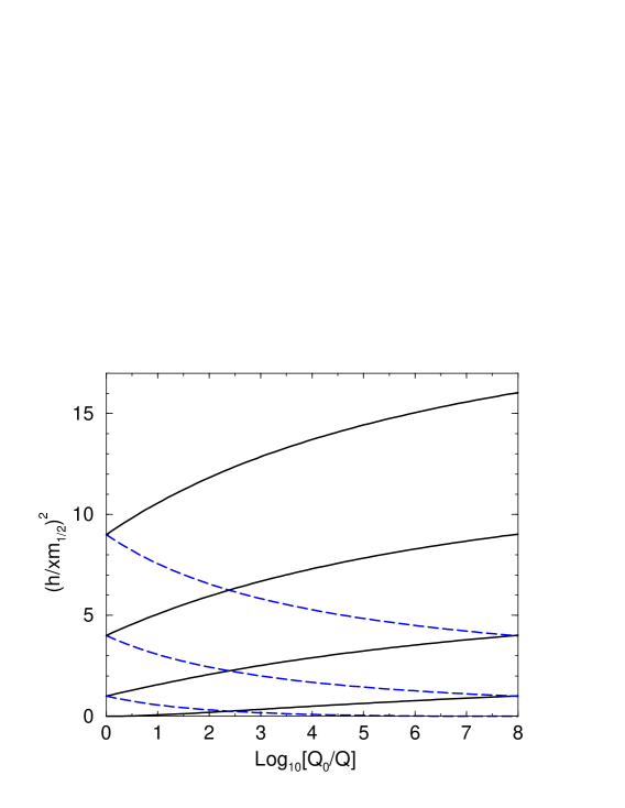
Figure 2: RG running of $h/xm_{1/2}$ for the minimal model of automatic $R$-parity conservation described in the text. Initial values at the high scale, corresponding to the left-hand side of the graph, are $h_{0}/x_{0}m_{1/2}=0,-1,-2,-3$ (solid lines) and $1,2,3$ (dashed lines).

Of course, the scalar masses $m_{S}^{2}$ and $m_{\overline{S}}^{2}$ are also running because of the $U(1)$ gauge couplings. This effect is quite significant because of the large ($\pm 2$) values of $B-L$ charges of the the $S,\overline{S}$ fields, and it opposes the symmetry breaking. Therefore, there is a competition between the magnitude of running for $m_{S}^{2}+m_{\overline{S}}^{2}$ and $|h/x|^{2}$ to decide whether an intermediate scale VEV can occur. As in section 3, this requires $|h/x|^{2}>6(m_{S}^{2}+m_{\overline{S}}^{2})$ at an intermediate scale. For a numerical example, one can use $g_{U}^{2}/4\pi=0.04$ and $Q_{0}/Q=10^{6}$ or $t_{0}-t=13.8$ in eqs. (4.15) and (4.17) to get $m_{S}^{2}=m_{\overline{S}}^{2}\approx m_{0}^{2}+0.33m_{1/2}^{2}$ and $h/x\approx h_{0}/x_{0}-0.88m_{1/2}$. In Figure 3, I show the regions of parameter space in the $h_{0}/x_{0}m_{1/2}$ vs. $m_{0}^{2}/m_{1/2}^{2}$ plane for which a non-trivial local minimum occurs along the $S,\overline{S}$ flat direction in this model. There is a local minimum for all values of $m_{0}^{2}/m_{1/2}^{2}$ below the lines indicated. The solid line corresponds to a ratio of the high scale to the intermediate scale of $10^{6}$, while the dashed line corresponds to the case of no renormalization of parameters (if the intermediate scale were pushed up close to the high scale, which can occur in the limit that $x$ is very small).

Figure 3: The parameter space in the $h_{0}/x_{0}m_{1/2}$ vs. $m_{0}^{2}/m_{1/2}^{2}$ plane for which a non-trivial local minimum occurs along the $S,\overline{S}$ flat direction in the model described in the text, neglecting Yukawa couplings. A local minimum exists for all values of $m_{0}^{2}/m_{1/2}^{2}$ below the lines shown. The solid line corresponds to a hierarchy of the high scale to the intermediate scale of $Q_{0}/Q=10^{6}$, while the dashed line corresponds to the case of no renormalization ($Q_{0}/Q=1$).

As Fig. 3 shows, the parameter space in which intermediate-scale symmetry breaking occurs is actually diminished by RG running for $h_{0}/x_{0}m_{1/2}\lower 3.01385pt\hbox{$\;\stackrel{{\scriptstyle\textstyle>}}{{\sim}}\;$}-2$, and is increased for $h_{0}/x_{0}m_{1/2}\lower 3.01385pt\hbox{$\;\stackrel{{\scriptstyle\textstyle<}}{{\sim}}\;$}-2$. If one assumes a boundary condition $m_{1/2}^{2}=3m_{0}^{2}$ as can happen in certain dilaton-dominated scenarios of supersymmetry breaking, then a non-trivial minimum at an intermediate scale requires $h_{0}/x_{0}m_{1/2}\lower 3.01385pt\hbox{$\;\stackrel{{\scriptstyle\textstyle<}}{{\sim}}\;$}-1.9$ or $\lower 3.01385pt\hbox{$\;\stackrel{{\scriptstyle\textstyle>}}{{\sim}}\;$}3.7$ in this picture.

The discussion above is somewhat conservative, in that we have not included possible negative RG contributions to $m_{S}^{2}$ and $m_{\overline{S}}^{2}$. One might imagine that one could increase the region of parameter space in which symmetry breaking occurs by including the effects of the Yukawa couplings ${\bf y}_{\nu}$ and ${\bf y}_{S}$ in eq. (4.3). The latter coupling will certainly act to decrease $m_{S}^{2}$ in the infrared, which clearly favors a VEV for $S$. However, the impact of these corrections is somewhat limited. For example, assuming one neutrino Yukawa coupling $y_{S}$ and its corresponding scalar cubic term $a_{S}$ dominate, the relevant beta functions are:

$$16\pi^{2}\beta(m_{S}^{2}) = |y_{S}|^{2}(m_{S}^{2}+2m^{2}_{\overline{\nu}})+|a_{S}|^{2}-8\sum_{a}g_{a}^{2}M_{a}^{2}C_{a}(S)$$ (4.18)

$$16\pi^{2}\beta(m_{\overline{\nu}}^{2}) = 2|y_{S}|^{2}(m_{S}^{2}+2m^{2}_{\overline{\nu}})+2|a_{S}|^{2}+\ldots-8\sum_{a}g_{a}^{2}M_{a}^{2}C_{a}(\overline{\nu})\phantom{xx}$$ (4.19)

where the ellipses in eq. (4.19) refer to additional positive-definite contributions from Yukawa couplings. A comparison of the terms in these two equations reveals that without additional interactions, it is quite difficult to arrange for $m_{S}^{2}$ to be driven negative without first driving ${m}_{\overline{\nu}}^{2}$ negative, since $C_{a}(S)=4C_{a}(\overline{\nu})$. Once this occurs, $m_{S}^{2}$ will receive large positive contributions from the $2|y_{S}|^{2}m_{\overline{\nu}}^{2}$ term in its beta function. One possible alternative is to allow $S$ and $\overline{S}$ to have superpotential Yukawa couplings to some heavy particles which also have gauge interactions with respect to some strongly-coupled gauge group. The soft squared masses of these new heavy scalars will be large and positive, and through Yukawa couplings can allow $m_{S}^{2}$ and/or $m_{\overline{S}}^{2}$ to be driven negative or at least smaller in the infrared, thus increasing the parameter space in which intermediate-scale symmetry breaking occurs. In any case, the contributions of the dimensionless supersymmetry-breaking terms are likely to be non-negligible, and always favor symmetry breaking.

5 Model with automatic $R$-parity conservation tied to a solution to the $\mu$ problem

In this section I consider an extension of the model in the previous section which also incorporates a solution to the $\mu$-problem together with an invisible axion of the type proposed in ref. [28]. In addition to the $U(1)_{B-L}$ gauge supermultiplet and $S,\overline{S}$ fields, introduce an additional pair of neutral chiral supermultiplets $N$ and $\overline{N}$. These fields are charged under a global anomalous Peccei-Quinn (PQ) symmetry [29] as shown in Table 2. When the fields $\langle N\rangle$ and $\langle\overline{N}\rangle$ get VEVs, they will spontaneously break this PQ symmetry, which is also explicitly broken by the QCD anomaly.

Table 2: Charges of Higgs fields in the model described in section 5. The $B-L$ and $Y$ symmetries are local, and the PQ symmetry is a global symmetry with a QCD anomaly.

$S$ $\overline{S}$ $N$ $\overline{N}$ $H_{u}$ $H_{d}$ $B-L$ $2$ $-2$ $0$ $0$ $0$ $0$ $Y$ $0$ $0$ $0$ $0$ $1/2$ $-1/2$ PQ $1$ $-1$ $-1$ $1$ $1$ $1$

x

As before, I will assume that superpotential mass terms are absent. The leading terms in the superpotential consistent with the symmetries in Table 2 can then be written as:

$$W={x_{1}\over 2M}S^{2}\overline{S}^{2}-{x_{2}\over M}S\overline{S}N\overline{N}+{x_{3}\over 2M}N^{2}\overline{N}^{2}+{x_{\mu}\over M}N^{2}H_{u}H_{d}.$$ (5.1)

The last term in eq. (5.1) becomes the $\mu$ term of the MSSM when $N$ obtains its VEV. Then $\langle N\rangle$ should be of order the intermediate scale $\sqrt{m_{W}M}$ for two distinct reasons; first in order to allow the effective contribution to $\mu=x_{\mu}\langle N\rangle^{2}/M$ to be of order $m_{W}$, and second to allow the PQ scale to fall within the window permitted by direct searches and astrophysical constraints [30].

Because we are looking for a minimum of the potential with $\langle S\rangle,\langle\overline{S}\rangle,\langle N\rangle,\langle\overline{N}\rangle\gg\langle H_{u}\rangle,\langle H_{d}\rangle$, the last superpotential term in eq. (5.1) is only a small perturbation on the dynamics that fixes the VEVs of $S,\overline{S},N,$ and $\overline{N}$. The relevant supersymmetric part of the scalar potential is therefore

$$V_{\rm SUSY} = {1\over M^{2}}(|S|^{2}+|\overline{S}|^{2})|x_{1}S\overline{S}-x_{2}N\overline{N}|^{2}+{1\over M^{2}}(|N|^{2}+|\overline{N}|^{2})|x_{3}N\overline{N}-x_{2}S\overline{S}|^{2}$$ (5.2)

$$+{g_{X}^{2}\over 2}(|S|^{2}-|\overline{S}|^{2})^{2},$$

and the supersymmetry-breaking terms are

$${V}_{\rm breaking} = \left({h_{1}\over 2M}S^{2}\overline{S}^{2}-{h_{2}\over M}S\overline{S}N\overline{N}+{h_{3}\over 2M}N^{2}\overline{N}^{2}\right)+{\rm c.c.}$$ (5.3)

$$+m_{S}^{2}|S|^{2}+m_{\overline{S}}^{2}|\overline{S}|^{2}+m_{N}^{2}|N|^{2}+m_{\overline{N}}^{2}|\overline{N}|^{2}.$$

The parameter space of this model is multidimensional and complicated, so I will be content to explore it quantitatively in some special cases. In order to simplify the analysis, I will assume that $x_{2}/x_{1}$ and $x_{3}/x_{1}$ are both real. Then each of $x_{1}$, $x_{2}$, and $x_{3}$ can be made real and positive by a field rephasing, without loss of generality. I will also assume that

$$h_{1}/x_{1}=h_{2}/x_{2}=h_{3}/x_{3}\equiv(h/x)_{0}$$ (5.4)

at the unification scale $Q_{0}$, and that all scalars have a common squared mass equal to $m_{0}^{2}$ at that same scale. RG equations are used to run the parameters $h_{1}/x_{1}m_{1/2}$, $h_{2}/x_{2}m_{1/2}$, $m_{S}^{2}/m_{1/2}^{2}$, and $m_{\overline{S}}^{2}/m_{1/2}^{2}$ to the intermediate scale $Q$ to evaluate the scalar potential. The ratios $h_{3}/x_{3}m_{1/2}$, $m_{N}^{2}/m_{1/2}^{2}$, and $m_{\overline{N}}^{2}/m_{1/2}^{2}$ involve gauge singlets and do not run. Then minima of the potential can be identified by a straightforward procedure. This involves numerically solving quartic and quadratic equations to find all possible candidate extrema, and then requiring that all of the eigenvalues of the Hessian matrix at the minimum are positive. The candidate minima occur near the $D$-flat direction $|\langle S\rangle|=|\langle\overline{S}\rangle|=s$. Furthermore, my assumption $m_{N}^{2}=m_{\overline{N}}^{2}$ implies that $|\langle N\rangle|=|\langle\overline{N}\rangle|=n$, because of an approximate symmetry $N\leftrightarrow\overline{N}$.

I have checked that for generic choices of $x_{1}/x_{3}$ and $x_{2}/x_{3}$, there are stable local minima for sufficiently large values of $(h/x)_{0}/m_{1/2}$ compared to $m_{0}^{2}/m_{1/2}^{2}$, just as for the model in the previous section. However, in the present case both $s$ and $n$ are non-zero. It is instructive to first consider the special case that $Q_{0}/Q=1$ so that there is no renormalization of parameters from the high scale. Then, at least for many values of $x_{1}/x_{3}$ and $x_{2}/x_{3}$, a stable local minimum exists provided that

$$(h/x)^{2}_{0}>12m^{2}_{0},$$ (5.5)

with $n^{2}/s^{2}=(x_{1}+x_{2})/(x_{3}+x_{2})$. For the more realistic case including renormalization effects, I have chosen to present results for the special case $x_{1}/x_{3}=4$ and $x_{2}/x_{3}=3$, and for case $x_{1}/x_{3}=1/4$ and $x_{2}/x_{3}=1/3$, in Fig. 4. (These ratios are taken to be specified at the intermediate scale.) For both models, the area below the dashed curve is the region of parameter space in which a local minimum exists when $Q_{0}/Q=1$, as in eq. (5.5). The area below the dash-dot line is the corresponding region for $Q_{0}/Q=10^{6}$ when $(x_{1}/x_{3},x_{2}/x_{3})=(4,3)$. Likewise, the area below the solid line is the region allowing intermediate scale VEVs for $Q_{0}/Q=10^{6}$ and $(x_{1}/x_{3},x_{2}/x_{3})=(1/4,1/3)$. I have checked that similar results obtain for many other choices of $x_{1}/x_{3}$ and $x_{2}/x_{3}$.

Figure 4: The parameter space in the $h_{0}/x_{0}m_{1/2}$ vs. $m_{0}^{2}/m_{1/2}^{2}$ plane for which a local minimum involving non-zero $\langle S\rangle=\langle\overline{S}\rangle$ and $\langle N\rangle=\langle\overline{N}\rangle$ occurs, for the model and RG boundary conditions described in section 5. At least one non-trivial local minimum exists for all values of $m_{0}^{2}/m_{1/2}^{2}$ below the lines shown. For a hierarchy of the high scale to the intermediate scale of $Q_{0}/Q=10^{6}$, the dash-dot line corresponds to the choice $x_{1}/x_{3}=4$ and $x_{2}/x_{3}=3$ and the solid line corresponds to $x_{1}/x_{3}=1/4$ and $x_{2}/x_{3}=1/3$. In the case of no renormalization $(Q_{0}/Q=1)$, both models have non-trivial local minima for all $m_{0}^{2}/m_{1/2}^{2}$ below the dashed line.

As Fig. 4 shows, the critical line for $(h/x)_{0}/m_{1/2}<0$ is surprisingly insensitive to renormalization group running. This is actually something of an accident, reflecting the fact that the scalar squared masses and $(h_{i}/x_{i})^{2}$ run at comparable rates. For the opposite sign of $(h/x)_{0}/m_{1/2}$, there is somewhat more sensitivity. Also, I find that for values of $m_{0}^{2}$ far below the critical lines shown, there are sometimes several distinct non-trivial local minima separated by “ridges” in field space. Note that the critical lines in this model are between the two lines shown in Figure 3. This can be understood as follows: along the flat direction $(n,s)$ chosen by the model in this section, the minimum is determined by effective $h$ and $x$ couplings which are, roughly speaking, “averages” of some couplings that are renormalized by $B-L$ interactions just as in section 4, and other couplings that are not renormalized because they are gauge singlets.

However, it is important to realize that the situation depicted in Fig. 4 is not inevitable, since the relationship between $h_{1}$, $h_{2}$, and $h_{3}$ can be relaxed. To see this, note that if the special (one-loop RG-invariant) relationship $x_{1}x_{3}=x_{2}^{2}$ were to hold, then there would be exactly flat directions of the supersymmetric part of the potential, eq. (5.2), with $|S|^{2}=|\overline{S}|^{2}$ and $N\overline{N}/S\overline{S}=x_{1}/x_{2}=x_{2}/x_{3}$. Now, with the boundary conditions on the $h_{i}/x_{i}$ discussed above, it happens that at one loop order the supersymmetry-breaking quartic part of the scalar potential is also flat at one-loop order. However, if one imagines relaxing this condition and allowing generic values of $h_{i}/x_{i}$, then the negative supersymmetry-breaking $h$-terms will dominate the scalar potential for field values slightly above the intermediate scale for some neighborhood of parameter space near $x_{1}x_{3}=x_{2}^{2}$. This makes it clear that for even for rather small, but generic, values of ($h_{1}$, $h_{2}$, $h_{3}$), there must always be at least some finite region of ($x_{1}$, $x_{2}$, $x_{3}$) parameter space near $x_{1}x_{3}=x_{2}^{2}$ in which the symmetry breaking does take place. I have checked that this region of parameter space can be quite large.

The model outlined above has the nice feature that it relates the PQ intermediate scale governed by $\langle N\rangle$ to the neutrino see-saw intermediate mass scale governed by $\langle S\rangle$. A similar model was proposed in ref. [31], but in that paper the mechanism for intermediate-scale symmetry breaking was supposed to be negative RG corrections to scalar squared masses. In the model described here, $B-L$ is gauged in order to provide for automatic $R$-parity conservation, and this makes it extremely difficult for negative scalar squared masses $m_{S}^{2}$ and $m_{\overline{S}}^{2}$ to arise. In any case, I have argued that the $h\phi^{4}$ coupling probably provides a significant part of the effect. If the physical neutrino masses are very small, it may be required that there is a mild hierarchy $\langle N\rangle\lower 3.01385pt\hbox{$\;\stackrel{{\scriptstyle\textstyle<}}{{\sim}}\;$}10^{12}$ GeV $\ll\langle S\rangle$ in order to accommodate the allowed axion window. This can be accomplished by choosing the couplings $x_{1},x_{2},x_{3}$ appropriately. In the model I have described, the intermediate scale symmetry breaking occurs even though no scalar squared mass runs negative, and without tuning the relative magnitudes of any superpotential terms. As is the case for the model in the previous section, matter parity is automatically a conserved symmetry because of the way $B-L$ is broken. In addition, the strong CP problem is solved and there is an invisible axion (which is mainly Im$[N-\overline{N}]/\sqrt{2}$) along the lines of ref. [28]. The fermionic axino and scalar saxino partners of the axion both obtain electroweak-scale masses, but they are only very weakly coupled to ordinary matter. As before, one expects that the pattern of MSSM squark and slepton masses will be augmented by a $B-L$ $D$-term contribution, which could be distinguished at the CERN Large Hadron Collider or a future lepton linear collider. As emphasized in section 3, the magnitude and even the sign of the $D$-term depend on non-renormalizable Kahler potential terms, but its existence is non-negotiable.

6 Conclusions

In this paper, I have studied the effects of supersymmetry-breaking $\phi^{4}$ couplings in producing intermediate-scale VEVs. Any truly complete model of supersymmetry breaking should be able to predict the magnitude of these terms, at least relative to the corresponding superpotential couplings. As shown in sections 2 and 3, these terms are most important in or near $D$-flat directions that are also $F$-flat at the renormalizable level. For these purposes, there is a well-defined procedure for including RG effects, as given by the beta function eq. (2.8), which incorporates the large logarithms in an effective potential approach.

An intermediate scale roughly of order $\sqrt{m_{W}M_{\rm Planck}}$ is suggested both by the see-saw scenario for neutrino masses and the allowed axion window [30]. In sections 4 and 5, I discussed simple models in which the existence of these scales is dependent on the presence of dimensionless supersymmetry-breaking terms. The numerical studies in this paper show that in the simplest cases, one requires the values of the dimensionless ratio $h/xm_{1/2}$ at the Planck scale to be fairly large, and perhaps to favor a particular sign, in order to achieve intermediate-scale symmetry breaking. However, this may well be too conservative since Figs. 3 and 4 neglect the possible effects of negative contributions to scalar squared masses from RG effects, even if the scalar squared masses never run negative. Furthermore, as I argued briefly in section 5, the parameter space in which intermediate-scale symmetry breaking can take place can be increased substantially if one is close to an accidental nearly-flat direction and the $h\phi^{4}$ terms are misaligned with the corresponding superpotential terms. In any case, it is likely that the dimensionless supersymmetry breaking couplings play a crucial role in producing VEVs along supersymmetric flat directions.

Acknowledgements: I thank Nir Polonsky, Pierre Ramond and James Wells for useful comments, and the Aspen Center for Physics for hospitality. This work was supported in part by National Science Foundation grant number PHY-9970691.

Appendix: flat directions in the MSSM

In this paper, I have mainly been concerned with the ability of dimensionless supersymmetry-breaking couplings to produce desired intermediate-scale VEVs like the PQ scale and the neutrino seesaw scale. It is also interesting to consider the opposite case, when we do not want an intermediate scale VEV to occur; namely, $h$-terms corresponding to flat directions in the MSSM. Supersymmetric flat directions are parameterized by analytic gauge-invariant polynomials in chiral superfields. For example, there are flat directions $QQQL$ and $\overline{u}\overline{u}\overline{d}\overline{e}$ which are not lifted by any renormalizable supersymmetric terms in the scalar potential. Instead, they are lifted by supersymmetry-breaking (mass)² terms, by non-renormalizable superpotential terms, and by the corresponding $h$-type terms. The latter terms always lower the scalar potential for some choice of phases of the fields, and therefore favor the existence of a non-trivial minimum at an intermediate scale. Naively, these minima are potentially dangerous, since they of course break color and electric charge. However, the mere existence of such vacua does not imply that the universe has to be in one of them in the present day, even if they are global minima. On the other hand, the dynamics associated with the flat directions may play an important role in the early universe, particularly during inflation when the relevant $F$-term may be the auxiliary component of the inflaton, and in the study of baryogenesis [32, 11]. Here, I will illustrate the importance of the RG running by considering the $h$-terms for the $\overline{u}\overline{u}\overline{d}\overline{e}$ flat directions. The analysis is very similar e.g. for the $QQQL$ flat directions.

The relevant superpotential is given by

$$W={x^{ijkl}\over 2M}\overline{u}_{i}\overline{u}_{j}\overline{d}_{k}\overline{e}_{i}$$ (A.1)

where gauge indices are suppressed in the only possible way and $i=1,2,3$ is a family index. The supersymmetry-breaking potential is given by

$$V={h^{ijkl}\over 2M}\overline{u}_{i}\overline{u}_{j}\overline{d}_{k}\overline{e}_{i}+{\rm c.c.}+\sum_{i=1}^{3}\left(m^{2}_{u_{i}}|\overline{u}_{i}|^{2}+m^{2}_{d_{i}}|\overline{d}_{i}|^{2}+m^{2}_{e_{i}}|\overline{e}_{i}|^{2}\right).$$ (A.2)

Now, suppose we are interested in a particular flat direction with $SU(3)_{C}$ color components

$$\overline{u}_{1}=\pmatrix{\phi\cr 0\cr 0};\qquad\overline{u}_{2}=\pmatrix{0\cr\phi\cr 0};\qquad\overline{d}_{1}=\pmatrix{0\cr 0\cr\phi};\qquad\overline{e}_{1}=\phi.$$ (A.3)

Here the indices $1$ and $2$ on $\overline{u}_{1}$, $\overline{u}_{2}$, $\overline{d}_{1}$ and $\overline{e}_{1}$ represent arbitrarily-labelled family components. The potential along the flat direction is given by

$$V=\sum m^{2}|\phi|^{2}+\left({h\over M}\phi^{4}+{\rm c.c.}\right)+{4\overline{x}^{2}\over M^{2}}|\phi|^{6},$$ (A.4)

where

$$\sum m^{2} \equiv m_{u_{1}}^{2}+m_{u_{2}}^{2}+m_{d_{1}}^{2}+m_{e_{1}}^{2};$$ (A.5)

$$h \equiv h^{1211};$$ (A.6)

$$\overline{x}^{2} \equiv {1\over 4}\sum_{i=1}^{3}\left(|x^{i211}|^{2}+|x^{1i11}|^{2}+|x^{12i1}|^{2}+|x^{121i}|^{2}\right).$$ (A.7)

In the MSSM, there are no Yukawa couplings which simultaneously link any pair of fields $\overline{u}$, $\overline{d}$ and $\overline{e}$. Furthermore, to a very good approximation, the Yukawa contribution to wavefunction renormalizations are only non-vanishing for the $t,b,\tau$ family. Therefore, the conditions leading to eq. (2.10) are satisfied, and one can write a simple RG equation for each separate ratio $h^{ijkl}/x^{ijkl}$:

$${d\over dt}(h/x)={g_{3}^{2}\over\pi^{2}}M_{3}+{3g_{1}^{2}\over 10\pi^{2}}M_{1}.$$ (A.8)

(I emphasize that this is true even when the coupling involves $t,b,\tau$ fields.) The resulting running of this family-independent ratio is graphed in Fig. 5, starting from unified gauge couplings at $Q_{0}=3\times 10^{16}$ GeV. As the graph shows, the ratio $(h/xm_{1/2})^{2}$ can become quite large for negative $h_{0}/x_{0}m_{1/2}$, while for positive $h_{0}/x_{0}m_{1/2}$ it tends to run to very small values.

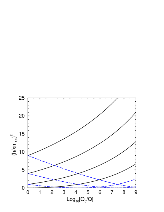
Figure 5: RG running of $h/xm_{1/2}$ for a $\overline{u}\overline{u}\overline{d}\overline{e}$ flat direction in the MSSM as described in the text. Initial values at the high scale (corresponding to the left-hand side of the graph) are $h/xm_{1/2}=0,-1,-2,-3$ (solid lines) and $h/xm_{1/2}=1,2,3$ (dashed lines).

A non-trivial local minimum in the scalar potential can occur at an intermediate scale if

$$|h|^{2}-3\overline{x}^{2}\sum m^{2}>0.$$ (A.9)

Note that while the RG running shown involves only the coupling $x$ corresponding to the gauge-invariant polynomial of the flat direction, the minimization condition that needs to be satisfied involves the larger averaged squared coupling $\overline{x}^{2}$. If only one coupling dominates, then $\overline{x}^{2}\approx x^{2}$. The relationship between $x^{2}$ and $\overline{x}^{2}$ is quite model-dependent; however, there are strong constraints on these couplings because they are dimension 5 proton decay operators. Therefore, it is probable that the largest of the couplings $x$ belong to the $t,b,\tau$ family, which are constrained the least by proton decay searches. In addition, the top and bottom squarks get negative RG corrections to their masses due to the top and bottom Yukawa couplings. Therefore, it is quite likely that if a non-trivial local minimum exists, it will involve the third-family quarks and sleptons. I find that such a minimum can easily exist for $h/xm_{1/2}\lower 3.01385pt\hbox{$\;\stackrel{{\scriptstyle\textstyle<}}{{\sim}}\;$}-2$ or so, because of the fast growth of $h/x$ in the infrared. However, the precise regions of parameter space in which this can occur depend on numerous unknown variables (including the scalar cubic couplings) so I will not attempt to outline them here.

References

- [1] H.P. Nilles, Phys. Rept. 110, 1 (1984); H.E. Haber and G.L. Kane, Phys. Rept. 117, 75 (1985).
- [2] S.P. Martin, “A Supersymmetry primer,” hep-ph/9709356.
- [3] K. Harada and N. Sakai, Prog. Theor. Phys. 67, 1877 (1982).
- [4] L. Girardello and M.T. Grisaru, Nucl. Phys. B194, 65 (1982).
- [5] K. Inoue, A. Kakuto, H. Komatsu and S. Takeshita, Prog. Theor. Phys. 68, 927 (1982), erratum ibid 70 330 (1983).
- [6] D.R.T. Jones, L. Mezincescu and Y.P. Yao, Phys. Lett. 148B, 317 (1984).
- [7] L.J. Hall and L. Randall, Phys. Rev. Lett. 65, 2939 (1990).
- [8] F. Borzumati, G.R. Farrar, N. Polonsky and S. Thomas, “Soft Yukawa couplings in supersymmetric theories,” hep-ph/9902443.
- [9] I. Jack and D.R.T. Jones, “Nonstandard soft supersymmetry breaking,” hep-ph/9903365.
- [10] F. Buccella, J.P. Derendinger, S. Ferrara and C.A. Savoy, Phys. Lett. 115B, 375 (1982); R. Gatto and G. Sartori, Phys. Lett. 157B, 389 (1985); M.A. Luty and W.I. Taylor, Phys. Rev. D53, 3399 (1996);
- [11] M. Dine, L. Randall and S. Thomas, Nucl. Phys. B458, 291 (1996).
- [12] T. Gherghetta, C. Kolda and S.P. Martin, Nucl. Phys. B468, 37 (1996).
- [13] G. Cleaver et al, Nucl. Phys. B545, 47 (1999).
- [14] S.P. Martin, Phys. Rev. D54, 2340 (1996).
- [15] G. Lazarides and Q. Shafi, Phys. Rev. D58, 071702 (1998).
- [16] I. Jack et al, Phys. Rev. D50, 5481 (1994).
- [17] M. Drees, Phys. Lett. 181B, 279 (1986).
- [18] J.S. Hagelin and S. Kelley, Nucl. Phys. B342, 95 (1990); A.E. Faraggi, J.S. Hagelin, S. Kelley and D.V. Nanopoulos, Phys. Rev. D45, 3272 (1992).
- [19] Y. Kawamura and M. Tanaka, Prog. Theor. Phys. 91, 949 (1994); Y. Kawamura, H. Murayama and M. Yamaguchi, Phys. Lett. B324, 52 (1994); Phys. Rev. D51, 1337 (1995).
- [20] H.C. Cheng and L.J. Hall, Phys. Rev. D51, 5289 (1995).
- [21] C. Kolda and S.P. Martin, Phys. Rev. D53, 3871 (1996).
- [22] G. Jungman, M. Kamionkowski and K. Griest, Phys. Rept. 267, 195 (1996); J. Ellis, T. Falk, K.A. Olive and M. Schmitt, Phys. Lett. B413, 355 (1997); J.D. Wells, “Mass density of neutralino dark matter,” hep-ph/9708285, in “Perspectives on Supersymmetry”, ed. G.L.Kane, World Scientific.
- [23] R.N. Mohapatra, Phys. Rev. D34, 3457 (1986); A. Font, L.E. Ibanez and F. Quevedo, Phys. Lett. B228, 79 (1989).
- [24] S.P. Martin, Phys. Rev. D46, 2769 (1992).
- [25] R. Kuchimanchi and R.N. Mohapatra, Phys. Rev. Lett. 75, 3989 (1995); Z. Chacko and R.N. Mohapatra, Phys. Rev. D58, 015001 (1998).
- [26] K. Huitu, P.N. Pandita and K. Puolamaki, Phys. Lett. B415, 156 (1997).
- [27] C.S. Aulakh, A. Melfo and G. Senjanovic, Phys. Rev. D57, 4174 (1998); C.S. Aulakh, A. Melfo, A. Rasin and G. Senjanovic, hep-ph/9902409.
- [28] J.E. Kim and H.P. Nilles, Phys. Lett. 138B, 150 (1984). Mod. Phys. Lett. A9, 3575 (1994).
- [29] R.D. Peccei and H.R. Quinn, Phys. Rev. Lett. 38, 1440 (1977).
- [30] J. Preskill, M.B. Wise and F. Wilczek, Phys. Lett. 120B, 127 (1983); L.F. Abbott and P. Sikivie, Phys. Lett. 120B, 133 (1983); M. Dine and W. Fischler, Phys. Lett. 120B, 137 (1983); M.S. Turner, Phys. Rept. 197, 67 (1990); G.G. Raffelt, Phys. Rept. 198, 1 (1990).
- [31] H. Murayama, H. Suzuki and T. Yanagida, Phys. Lett. B291, 418 (1992).
- [32] I. Affleck and M. Dine, Nucl. Phys. B249, 361 (1985).