NORDITA-99/45HE

MCGILL-99/22

NBI-HE-99-25

hep-ph/9907545

CHERN-SIMONS NUMBER DIFFUSION AND HARD THERMAL LOOPS ON THE LATTICE

D. Bödeker^a,, Guy D. Moore^b, and K. Rummukainen^c,d,

^aNiels Bohr Institute, Blegdamsvej 17, DK-2100 Copenhagen Ø, Denmark
^bDept. of Physics, McGill University, 3600 University St., Montreal, PQ H3A 2T8 Canada
^cNordita, Blegdamsvej 17, DK-2100 Copenhagen Ø, Denmark
^dHelsinki Institute of Physics, P.O.Box 9, 00014 University of Helsinki, Finland

Abstract

We develop a discrete lattice implementation of the hard thermal loop effective action by the method of added auxiliary fields. We use the resulting model to measure the sphaleron rate (topological susceptibility) of Yang-Mills theory at weak coupling. Our results give parametric behavior in accord with the arguments of Arnold, Son, and Yaffe, and are in quantitative agreement with the results of Moore, Hu, and Müller.

PACS: 11.10.Wx, 11.15.Ha, 12.60.Jv, 98.80.Cq
Keywords:
finite temperature, baryon number violation, electroweak phase transition, lattice simulations

1 Introduction

Baryon number is not a conserved quantity in the standard model. Rather, because of the anomaly, its violation is related to the electromagnetic field strength of the weak SU(2) group [1],

$$\partial_{\mu}J^{\mu}_{B}=N_{G}\frac{g^{2}}{32\pi^{2}}\epsilon_{\mu\nu\alpha\beta}{\rm Tr}F^{\mu\nu}F^{\alpha\beta}=N_{G}\frac{g^{2}}{8\pi^{2}}E_{i}^{a}B_{i}^{a}\,,$$ (1.1)

where $N_{G}=3$ is the number of generations. In vacuum the efficiency of baryon number violation through this mechanism is totally negligible [1], but at a sufficiently high temperature this is no longer true [2, 3]. This can have very interesting cosmological significance, since it complicates GUT baryogenesis mechanisms and opens the possibility of baryogenesis from electroweak physics alone. This motivates a careful investigation of baryon number violation in the standard model at high temperatures.

The baryon number violation rate relevant in cosmological settings can be related by a fluctuation dissipation relation [4, 5, 6] to the “Minkowski topological susceptibility” of the electroweak theory, also called the “sphaleron rate,”

$$\Gamma\equiv\int d^{3}x\int_{-\infty}^{\infty}dt\left(\frac{g^{2}}{8\pi^{2}}\right)^{2}\langle[E_{i}^{a}B_{i}^{a}(x,t)]\>[E_{j}^{b}B_{j}^{b}(0,0)]\rangle\,,$$ (1.2)

where $\langle\rangle$ means an expectation value with respect to the equilibrium thermal density matrix. Here $t$ is Minkowski time. This quantity is not simply related to the Euclidean topological susceptibility [7], and we do not possess either perturbative tools or Euclidean tools to carry out its calculation.

It has been argued by Grigoriev and Rubakov [8] that the value of the susceptibility $\Gamma$ in the quantum theory will be the same as its value in classical Yang-Mills field theory. This would open a new avenue for measuring $\Gamma$, since classical Yang-Mills theory can be put on the lattice [9]. There has been some progress on measuring $\Gamma$ on the lattice [10, 11, 12, 13]; in particular two different methods have been developed for dealing with the right hand side of Eq. (1.2) in a topological way which eliminates lattice artifacts in its measurement [14, 15].

At the same time our qualitative understanding of Grigoriev and Rubakov’s claim has improved. A complication with their proposal is that 3+1 dimensional classical Yang-Mills theory contains ultraviolet (UV) divergences, which Bödeker, McLerran, and Smilga have argued may be important in setting $\Gamma$ [16]. Subsequently, Arnold, Son, and Yaffe have demonstrated that a particular class of diagrams, the hard thermal loops (HTL’s), are essential to establishing $\Gamma$ [17]. The amplitude of the HTL’s in the classical theory is linearly divergent, and therefore linearly cutoff dependent. In the full quantum theory the HTL’s are finite, with almost all of the contribution arising from excitations with momentum $k\simeq\pi T$; such high $k$ excitations are not properly described by the classical theory. Arnold, Son, and Yaffe argue that because of the HTL’s, the effective infrared (IR) theory “feels” the “cutoff” which quantum mechanics provides for the classical theory, and that the value of $\Gamma$ scales inversely with the cutoff momentum scale. As a result, rather than the naive dimensional estimate of $\Gamma\sim\alpha^{4}T^{4}$, the parametric behavior of $\Gamma$ should be $\Gamma\sim\alpha^{5}T^{4}$; and in particular $\Gamma$ is inversely proportional to the strength of the HTL’s, which is conveniently parameterized by the Debye mass squared $m_{\rm D}^{2}$. On the lattice this means that $\Gamma$ should depend on the lattice spacing $a$ as $\Gamma\propto ag^{2}T\alpha^{4}T^{4}$, a behavior which has recently been verified numerically [18]. Arnold, Son, and Yaffe’s argument has been carefully re-analyzed by Bödeker, who has shown that there is an additional, logarithmic dependence on the Debye mass, and that, permitting an expansion in $\log(1/g)\gg 1$, the leading behavior is actually $\Gamma\sim\alpha^{5}\log(1/g)T^{4}$ [19].

If we take the limit $\log(1/g)\gg 1$, Bödeker presents an effective theory for evaluating the coefficient of the $\alpha^{5}\log(1/g)T^{4}$ law [19]. The effective theory is UV safe [20] and the coefficient can be found accurately by lattice means [21]. However, in practice the expansion in $\log(1/g)\gg 1$ turns out to be very poorly behaved. To get a reasonably accurate value for $\Gamma$ at the physical value for the electroweak coupling, $\alpha\simeq 1/30$, it is necessary to treat the dynamics of the classical field theory with a full inclusion of the HTL effects. This is challenging, because the HTL effective action is nonlocal [22]. However, it is possible to rewrite the HTL action in terms of a local theory with added degrees of freedom, as we will discuss below. Thus, it could be possible to determine $\Gamma$ by measuring the topological susceptibility of lattice regulated, classical Yang-Mills theory, supplemented by added degrees of freedom which correctly generate the hard thermal loop effects. Doing so would both test Arnold, Son, and Yaffe’s claim, and determine the numerical coefficient of the $\alpha^{5}T^{4}$ law, and therefore tell us how efficiently baryon number is violated at high temperatures.

One way of realizing this goal was presented in [23] and implemented and used to measure $\Gamma$ in [24]. The purpose of this paper is to present an alternative and in some respects more efficient implementation of classical Yang-Mills theory plus hard thermal loops, and to use it to check the results of [24]. Our approach is based on a way of writing the hard thermal loops in terms of auxiliary fields which was first proposed in [25]. Using this formulation to incorporate the HTL action on the lattice has been advocated by Bödeker, McLerran, and Smilga [16]. This paper represents a concrete numerical realization of that idea.

In Section 2 we review the local formulation of classical Yang-Mills field theory supplemented by the HTL action due to Blaizot and Iancu and due to Nair. Their theory contains an infinite set of fields, so in Section 3 we perform a transformation and a truncation to make the number of fields in the model finite, without losing spherical symmetry. The resulting theory does not quite give the correct HTL equations of motion; we study the difference, and how it vanishes in the limit as the truncation leaves in more and more fields, in Section 4. Then we discretize space and time in Section 5, and review how to measure $\Gamma$ topologically in Section 6. We study the numerical behavior of $\Gamma$ as a function of the strength of the HTL’s and the truncation point in Section 7.

Our conclusions are in Section 8, but we summarize them here. The HTL effective theory shows a dependence on the strength of HTL’s which is consistent with Arnold, Son, and Yaffe’s arguments, and grossly inconsistent with HTL independence. The dependence on the truncation point is surprisingly weak, so only a few new fields need to be added to approximate the correct HTL behavior. Thus, our algorithm proves quite an efficient way of incorporating HTL’s. Our final results for $\Gamma$ are consistent with those of Moore, Hu, and Müller [24], and for the physical value of $m_{\rm D}^{2}$ in the minimal standard model, $m_{\rm D}^{2}=(11/6)g^{2}T^{2}$ and $\alpha=1/30$, they give approximately $\Gamma=(25.4\pm 2.0)\,\alpha^{5}T^{4}$.

2 Hard thermal loops in the continuum

In this section we discuss the origin of the hard thermal loops in terms of kinetic theory, and we present a local theory in which extra degrees of freedom generate the hard thermal loops. Nothing in this section is original; rather it is a review of Blaizot and Iancu’s and of Nair’s work [25, 26, 27, 28]. We include it for completeness and because our numerical implementation of classical Yang-Mills theory with hard thermal loops will be built directly from it.

Two controlled approximations make the dynamics of IR fields in the electroweak theory tractable numerically, and both arise because the theory is weakly coupled. First, the IR degrees of freedom can to a good approximation be treated as classical fields. Using this fact to perform calculations of nonperturbative IR correlators was first proposed by Grigoriev and Rubakov [8], and the accuracy of the approximation has been addressed in [16, 29, 30]. The conclusion of [30] is that the classical approximation is an excellent approximation in the infrared, but UV divergences in the classical theory are potentially dangerous and must be handled carefully.

The solution to this problem is to regulate the classical theory in some way, which for the moment we will not specify, and then to treat the UV degrees of freedom separately by perturbation theory. Here the other controlled approximation enters; the UV degrees of freedom are described by linearized kinetic theory, up to corrections subleading in $g$.

Since the equilibrium distribution of UV modes, $N_{0}({\bf k})$, is color neutral, it does not directly enter in the field equations of the classical IR fields. Rather, it is necessary to expand the UV mode distribution function (one particle density matrix) up to first order in fluctuations from equilibrium,

$$N(x,{\bf k})=N_{0}({\bf k})+\delta N_{\rm singlet}(x,{\bf k})+\delta N_{\rm adj.}(x,{\bf k})+\ldots\,.$$ (2.1)

Fields in a representation higher than fundamental lead, in addition to the singlet and adjoint representation terms we have written, to higher representation departures from equilibrium; but neither these, nor the singlet deviation from equilibrium $\delta N_{\rm singlet}$, directly interact with the IR classical fields, and at the linearized level they can be dropped; only $N_{0}$ and $\delta N_{\rm adj.}$ will be relevant. Note also that $N$ should have a spin index, and if there are scalar or fermionic degrees of freedom then it also has a species index. At leading order, corresponding to the HTL approximation, the contribution from each spin and species are of the same form except in the statistics for $N_{0}$, so we will not write them in what follows.

At leading order in the coupling the IR classical fields evolve under the Yang-Mills field equations with a source arising from the UV modes, [25]

$$(D^{\nu}F_{\nu\mu})^{a} = j_{\mu}^{a}\,,$$ (2.2)

$$j_{\mu}^{a}(x) = 2gC_{A}\int\frac{d^{3}k}{(2\pi)^{3}}v_{\mu}\delta N^{a}(x,{\bf k})\,,$$ (2.3)

with $v^{\mu}=(1,{\bf v})$, ${\bf v}={\bf k}/|{\bf k}|$ the (ultrarelativistic) 3-velocity of the particles (note that $v^{\mu}$ is not a Lorentz covariant quantity), and $C_{A}=2$ for SU(2) gauge theory. We have only written the contribution of gauge excitations here, there are additional terms of the same form for scalars and fermions where appropriate. The distribution function evolves via a convective covariant derivative equation which reflects the ultrarelativistic propagation of the UV degrees of freedom. The interactions between $\delta N_{a}$ and the IR classical field strength is subdominant because the coupling is weak; however, the electric field polarizes the equilibrium distribution, providing a source term for $\delta N_{a}$. The equation for the evolution of $\delta N^{a}$, at leading order in $g$, is

$$\frac{{\rm d}\delta N^{a}}{{\rm d}t}=(v_{\mu}D^{\mu}_{x})^{ab}\delta N^{b}(x,{\bf k})+gv_{\mu}F_{0\mu}^{a}(x)\frac{\partial N_{0}}{\partial|{\bf k}|}=0\,.$$ (2.4)

Note that this equation is not Lorentz covariant; it involves only the electric field, not the magnetic field. The reason is that the equilibrium distribution $N_{0}$ has a rest frame. A magnetic field in that frame changes trajectories of individual particles, but it does not disturb the (rotationally symmetric) equilibrium distribution, whereas an electric field polarizes the plasma.

One approach to making a numerical model for the IR classical fields plus UV modes is to simulate the distribution function $N$ with a large number of charged particle degrees of freedom. In the limit that the number of particles is large and their charges are small, one recovers the above equations. This is the approach proposed by [23] and implemented in [24]. Here we will deal instead with the distribution functions. This complementary approach can test the reliability of the results of [24] and may also prove simpler and more efficient. This is particularly true because Eqs. (2.3) and (2.4) carry extra redundant information; $\delta N^{a}$ is actually a function of $\hat{{\bf k}}$ times a fixed function of $|{\bf k}|$, namely, [26, 27]

$$\delta N^{a}(x,{\bf k})=-g\frac{\partial N_{0}}{\partial|{\bf k}|}W^{a}(x,{\bf v})\,,$$ (2.5)

where ${\bf v}=\hat{{\bf k}}$ takes on values over the unit sphere. In terms of $W$, the convective evolution of the departure from equilibrium is

$$(v_{\mu}D^{\mu})^{ab}W^{b}(x,{\bf v})=v^{\mu}F_{0\mu}^{a}(x)\,,$$ (2.6)

and the current felt by the IR classical fields is

$$j_{\mu}^{a}(x)=m_{\rm D}^{2}\int\frac{d\Omega_{v}}{4\pi}v_{\mu}W^{a}(x,{\bf v})\,,$$ (2.7)

where $d\Omega_{v}$ means that ${\bf v}$ is integrated over the unit sphere with its natural measure. Here $m_{\rm D}^{2}$ is the square of the Debye mass. These equations can be viewed as generalized Hamilton-Jacobi equations arising from the conserved energy

$$H=\int d^{3}x\left(\frac{1}{4}F_{ij}^{a}F_{ij}^{a}+\frac{1}{2}F_{01}^{a}F_{01}^{a}+{\textstyle{\frac{1}{2}}}m_{\rm D}^{2}\int\frac{d\Omega_{v}}{4\pi}W^{a}(x,{\bf v})W^{a}(x,{\bf v})\right)\,,$$ (2.8)

and rather nontrivial Lie-Poisson brackets [28]. Here $\Omega_{v}$ is the integration measure for integrating ${\bf v}$ over the sphere.

When there are more than one species, $W^{a}$ represents the deviation from equilibrium felt by each, and $m_{\rm D}^{2}$ is a sum of a contribution from each species of charge carrier,

$$m_{\rm D}^{2}=g^{2}T^{2}\left(\frac{N}{3}+\frac{N_{s}}{6}+\frac{N_{f}}{12}\right)\,,$$ (2.9)

with $N_{s}$ the number of fundamental representation, complex scalars and $N_{f}$ the number of fundamental representation, chiral fermions. In the SU(2) weak sector of the minimal standard model, $N=2$, $N_{s}=1$, and $N_{f}=12$, so $m_{\rm D}^{2}=(11/6)g^{2}T^{2}$. This is also a lower bound for all extensions of the standard model.

Our approach will be to find a discrete implementation of Eqs. (2.3), (2.6), and (2.7), and to study their evolution to determine the diffusion constant for Chern-Simons number.

3 Expansion in Spherical Harmonics

Unfortunately, the representation of the hard thermal loops in terms of $W^{a}(x,{\bf v})$ does not provide a set of equations which are easy to implement numerically. The problem is that $W^{a}(x,{\bf v})$ is a function not only of space-time, but also over the sphere. Even if we discretize space onto a lattice, $W$ still “lives” on a sphere at each lattice point, so it still takes an infinite amount of information to specify $W$ completely. It is necessary to define $W$ over the sphere in some way requiring only a finite number of degrees of freedom. Since we want to recover spherical symmetry on scales long compared to our lattice spacing, we should choose to do so in a spherically symmetric way. Our choice is to expand $W$ in spherical harmonics,

$$W^{a}(x,{\bf v})=\sum_{l=0}^{\infty}\sum_{m=-l}^{l}W_{lm}^{a}(x)Y_{lm}({\bf v})\,,$$ (3.1)

where $W_{lm}^{a}(x)$ is a function over space-time only. Because $W^{a}(x,{\bf v})$ is real valued, the $W_{lm}^{a}$ satisfy the relations

$$W^{a}_{lm}=(-1)^{m}W^{a*}_{l,-m}\,,$$ (3.2)

so only the real part of $W_{l0}$, and the real and imaginary parts of $W_{lm}$ for $m>0$, should be viewed as independent variables. Here we use the Condon-Shortley phase convention and normalize $Y_{lm}$ so that

$$\int{d\Omega}\,Y^{*}_{lm}Y_{l^{\prime}m^{\prime}}=\delta_{l,l^{\prime}}\delta_{m,m^{\prime}}\,.$$ (3.3)

Inserting the expansion (3.1) into Eq. (2.6), multiplying by $Y^{*}_{lm}$, and integrating over angles, gives the equation of motion for $W_{lm}^{a}$,

$$\frac{\partial W^{a}_{lm}}{\partial t}=-C_{lm,l^{\prime}m^{\prime},i}\,\,(D_{i})^{ab}W^{b}_{l^{\prime}m^{\prime}}+\delta_{l,1}v_{mi}E_{i}^{a}\,,$$ (3.4)

where $v_{mi}$ is the vector ${\bf v}$ expressed in spherical components

$$v_{mi}=\int{d\Omega_{v}}Y^{*}_{1m}({\bf v})v_{i}$$ (3.5)

and $C_{lm,l^{\prime}m^{\prime},i}$ is an integral over 3 spherical harmonics:

$$C_{lm,l^{\prime}m^{\prime},i}=\int{d\Omega_{v}}Y^{*}_{lm}({\bf v})v_{i}Y_{l^{\prime}m^{\prime}}({\bf v})\,.$$ (3.6)

We give explicit expressions for $v_{mi}$ and $C_{lm,l^{\prime}m^{\prime},i}$ in Appendix A.

Furthermore, in terms of the spherical components the current is

$$j_{i}^{a}={\frac{m_{\rm D}^{2}}{4\pi}}v^{*}_{mi}W_{1m}^{a}\,,\qquad j_{0}^{a}={\frac{m_{\rm D}^{2}}{\sqrt{4\pi}}}W_{00}^{a}\,,$$ (3.7)

and the conserved energy density is

$$H=\int d^{3}x\left(\frac{1}{2}(E_{i}^{a}E_{i}^{a}+B_{i}^{a}B_{i}^{a})+{\frac{1}{2}}{\frac{m_{\rm D}^{2}}{4\pi}}\sum_{lm}|W^{a}_{lm}|^{2}\right)\,.$$ (3.8)

As written, Eqs. (3.4), (3.7), and (3.8) are equivalent to Eqs. (2.6), (2.7), and (2.8). They still contain an infinite number of degrees of freedom. However, they are in a form more amenable to a spherically symmetric truncation.

The meaning of $m_{\rm D}^{2}W^{a}(x,{\bf v})$ is that it represents the net charge of all excitations moving in the ${\bf v}$ direction at point $x$. What we have done is to transform to angular moments. $m_{\rm D}^{2}W^{a}_{00}(x)$ is the total charge of all excitations at site $x$. $m_{\rm D}^{2}W^{a}_{10}(x)$ is roughly the net charge moving in the $+z$ direction minus charge moving in the $-z$ direction, and $m_{\rm D}^{2}W^{a}_{lm}$ with $l\geq 2$ represent higher tensor moments in the distribution of excitations. For instance, a positive $m_{\rm D}^{2}W^{a}_{20}$ means, roughly, that there are more charges of type $a$ moving either up or down the $z$ axis than in the $x,y$ plane. Note that only $W_{00}^{a}$ and $W_{1m}^{a}$ interact with the IR fields, and only $W_{1m}^{a}$ is directly sourced by those fields. All the higher moments are important only in propagating the charge distribution through the convective derivative term in Eq. (3.4).

The model still contains a countably infinite number of degrees of freedom, namely $W^{a}_{lm},$ $l=1,2,3,\ldots$ . Most of these degrees of freedom are describing extremely subtle, high tensor fluctuations in the distribution of moving charges. It is reasonable to think that smearing the angular resolution of the distribution of charges by truncating the series of $Y_{lm}$ at some finite $l_{\rm max}$ will not significantly change the physics. In particular, for $l_{\rm max}\geq 1$ it will not change the way the charge current interacts with the Yang-Mills fields, but only the way the charges propagate; and for sufficiently large $l_{\rm max}$ we expect the effect of angular smearing to be unimportant. Therefore, to render the set of fields finite, we truncate the series of $W_{lm}^{a}$ at some finite $l_{\rm max}$. The evolution equation for $W_{lm}^{a}$ is still Eq. (3.4), but with all $W_{l^{\prime}m^{\prime}}^{a}$ with $l^{\prime}>l_{\rm max}$ fixed to zero. Equivalently, we could set all $C_{lm,l^{\prime}m^{\prime},i}$ with either $l>l_{\rm max}$ or $l^{\prime}>l_{\rm max}$ to zero. The number of independent adjoint $W_{lm}$ matrices is $(l_{\rm max}+1)^{2}$.

As long as $C_{lm,l^{\prime}m^{\prime},i}$ satisfies the relation

$$C_{lm,l^{\prime}m^{\prime},i}=C^{*}_{l^{\prime}m^{\prime},lm,i}$$ (3.9)

and the terms involving $v_{mi}$ are either both present or both absent (they are absent if $l_{\rm max}=0$), then the Hamiltonian, Eq. (3.8), and the phase space measure are conserved by the evolution equations. Hence it makes sense to speak of equal and unequal time, equilibrium thermal correlation functions. When $l_{\rm max}$ is finite we are no longer considering a theory which is strictly equivalent to classical Yang-Mills field theory with added hard thermal loops, but the behavior should approach the correct behavior in the limit $l_{\rm max}\rightarrow\infty$ and we can consider taking this limit numerically.

4 Propagator and Thermodynamics at Finite $l_{\rm max}$

Before moving on to the numerical implementation of the effective theory described in the last section in discrete space, we should pause to see how well or how badly the theory with finite $l_{\rm max}$ cutoff reproduces the hard thermal loops. To do so we first look at whether it reproduces them correctly at the thermodynamic level; it does so perfectly for all $l_{\rm max}\geq 0$. Then we examine the propagator of the theory, which will only be reproduced properly in the $l_{\rm max}\rightarrow\infty$ limit.

4.1 Thermodynamics

As discussed at the end of the last section, the theory with an $l_{\rm max}$ cutoff possesses well defined thermodynamics described by a Hamiltonian which is quadratic and diagonal in the $W_{lm}$’s. The only complication is that the phase space is constrained due to Gauss’ law:

$$(D\cdot E)^{a}=\frac{m_{\rm D}^{2}}{\sqrt{4\pi}}W^{a}_{00}\,,$$ (4.1)

and the partition function reads

$$Z = \int{\cal D}A_{i}{\cal D}E_{i}{\cal D}W_{lm}\delta\left((D\cdot E)^{a}-m_{\rm D}^{2}W^{a}_{00}/\sqrt{4\pi}\right)\exp(-H/T)\,,$$ (4.2)

$$H = \frac{1}{2}\int d^{3}x\left(B^{a}_{i}B^{a}_{i}+E^{a}_{i}E^{a}_{i}+\frac{m_{\rm D}^{2}}{4\pi}\sum_{lm}|W^{a}_{lm}|^{2}\right)\,.$$ (4.3)

Every $W_{lm}$ except $W_{00}$ is Gaussian and they can all be integrated out immediately. It is also convenient to introduce a Lagrange multiplier for Gauss’ law,

$$\delta\left((D\cdot E)^{a}-m_{\rm D}^{2}W^{a}_{00}/\sqrt{4\pi}\right)=\int{\cal D}A_{0}\exp\left\{iA^{a}_{0}\left[(D\cdot E)^{a}-m_{\rm D}^{2}W^{a}_{00}/\sqrt{4\pi}\right]/T\right\}\,.$$ (4.4)

Doing so makes $E$ and $W_{00}$ Gaussian as well, and they can now be integrated out, yielding

$$Z = \int{\cal D}A_{i}{\cal D}A_{0}\exp(-H^{\prime}/T)\,,$$ (4.5)

$$H^{\prime} = \frac{1}{2}\int d^{3}x\left[B_{i}^{a}B_{i}^{a}+(D_{i}A_{0})^{a}(D_{i}A_{0})^{a}+m_{\rm D}^{2}A_{0}^{a}A_{0}^{a}\right]\,,$$ (4.6)

where the wave function term for $A_{0}$ arises from integrating out the $E$ field and the Debye mass squared term arises from integrating out $W_{00}$.

The sole thermodynamic consequence of the $W$ fields is the introduction of a Debye mass, and its magnitude is given exactly by the coefficient in the $W$ field equations of motion. This corresponds exactly with what the complete hard thermal loop thermodynamic contribution should be. Furthermore, the Debye mass is introduced even for $l_{\rm max}=0$, the absolute minimum value. We do not recommend using $l_{\rm max}=0$, however, because in this case the $W$ fields have no dynamics and every $W^{a}_{00}$ is a conserved quantity. Therefore, the system is not ergodic and a Hamiltonian trajectory will not densely sample the microcanonical ensemble. However, to the best of our knowledge the only conserved quantities (besides the Gauss constraints) in the non-abelian theory with $l_{\rm max}\geq 1$ are energy and momentum, and we expect ergodicity in this case. The conclusion is that the technique reproduces the thermodynamics of the full HTL theory exactly, for all $l_{\rm max}\geq 1$.

4.2 Propagator

Now we turn to the study of the propagator in the $l_{\rm max}$ cut-off theory. We work only to linear order, or equivalently, we will study the propagator only in the abelian theory. In this case we can study one ${\bf k}$ mode in isolation.

Since the spherical harmonic expansion does not break rotational invariance (even when we restrict $l\leq l_{\rm max}$), it is sufficient to study the propagation of modes for which ${\bf k}$ is in the 3-direction. The Fourier transformed equations of motion are

$$\omega^{2}A_{m}-k^{2}A_{m} = {\frac{m_{\rm D}^{2}}{3}}W_{1m}$$ (4.7)

$$\omega W_{lm}-kC_{lm,l^{\prime}m^{\prime},3}W_{l^{\prime}m^{\prime}} = \omega\delta_{l,1}A_{m}\,,$$ (4.8)

where we have defined $A_{m=\pm 1}=\sqrt{4\pi/6}(\mp A_{1}+iA_{2})$ and $A_{m=0}=\sqrt{4\pi/3}A_{3}$. The $A_{\pm 1}$ are the transverse components of the gauge field and $A_{m=0}$ is longitudinal.

Since $C_{lm,l^{\prime}m^{\prime},3}\propto\delta_{m,m^{\prime}}$, c.f. Eq. (A.4), the equations of motion do not mix different $m$-sectors (this is the advantage of choosing ${\bf k}\parallel\hat{e}_{3}$). We also note that $W_{l_{\rm max}l_{\rm max}}$ and $W_{l_{\rm max},-l_{\rm max}}$ do not evolve at all. In general, the components with $m\neq\pm 1$ do not couple to the transverse gauge fields. We will not be concerned here with the propagator in the longitudinal sector, or with any sector which does not couple to any gauge fields, so the only ‘interesting’ modes are those with $m=\pm 1$. It should be noted that this decoupling occurs only  in the abelian theory. (It also allows a more efficient representation for hard thermal loops than the one we use here, see [31].)

In the following we choose $m=1$, which is the sector which couples to the transverse gauge fields. The matrix $C_{ll^{\prime}}=C_{l1,l^{\prime}1,3}$ is a symmetric and traceless matrix of size $l_{\rm max}^{2}$ with non-zero (positive) elements only if $l^{\prime}=l\pm 1$. (Note that, because $|m|\leq l$, $l$ is restricted here to the interval $1\leq l\leq l_{\rm max}$, hence the dimensionality of $C_{ll^{\prime}}$.) As a result, in the eigenvalue problem

$$C\chi^{\alpha}=\lambda^{\alpha}\chi^{\alpha}\,,$$ (4.9)

the eigenvalues $\lambda^{\alpha}$ are real and non-degenerate, and they come in positive and negative pairs: if $\lambda$ is an eigenvalue, so is $-\lambda$. If $l_{\rm max}$ is odd, the matrix has one zero eigenvalue, otherwise the eigenvalues are non-zero. The eigenvectors $\chi^{\alpha}$ are real and orthogonal, and we will normalize them to be orthonormal.

Writing the matrix $C_{ll^{\prime}}$ in terms of the eigenvectors and eigenvalues,

$$C_{ll^{\prime}}=\sum_{\alpha}\chi_{l}^{\alpha}\lambda^{\alpha}\chi_{l^{\prime}}^{\alpha}\,,$$ (4.10)

we can solve for $W_{l1}$ in Eq. (4.8):

$$W_{l1}=\sum_{\alpha}{\frac{\omega}{\omega-k\lambda^{\alpha}}}\chi_{l}^{\alpha}\chi_{1}^{\alpha}A_{1}\,.$$ (4.11)

Inserting this in Eq. (4.7), we obtain the inverse transverse propagator

$$\Delta^{-1}_{l_{\rm max}}=-\omega^{2}+k^{2}+{\frac{m_{\rm D}^{2}}{3}}\sum_{\alpha=1}^{l_{\rm max}}{\frac{\omega}{\omega-k\lambda^{\alpha}}}(\chi_{1}^{\alpha})^{2}\,.$$ (4.12)

Let us now compare the propagator (4.12) to the theory without  the $l$-cutoff. Remember that in this case the propagator has a cut in the interval $-k\leq\omega\leq k$ [32], and, in the limit $\omega\ll k\ll m_{\rm D}$, it describes overdamped  behavior with damping coefficient $\tau^{-1}\sim k^{3}/m_{\rm D}^{2}$. Thus, the damping rate is $\sim g^{4}T$ when $k\sim g^{2}T$, which is the relevant momentum scale for non-perturbative physics.

What does the propagator look like at different values of $l_{\rm max}$? If $l_{\rm max}=0$, the gauge fields are decoupled from the $W$ fields, except through Gauss’ law (see Eqs. (2.3) and (3.7)); transverse physics is the same as in the absence of the $W$ fields. At $l_{\rm max}=1$ the “matrix” $C_{ll^{\prime}}=0$ is a scalar, and the propagator describes a massive vector particle: $\Delta^{-1}_{1}=-\omega^{2}+k^{2}+m_{\rm D}^{2}/3$.

The first interesting case is $l_{\rm max}=2$. The propagator is still easy to solve analytically, and (using Eq. (A.4)) the inverse propagator becomes

$$-\omega^{2}+k^{2}+{\frac{m_{\rm D}^{2}}{3}}{\frac{\omega^{2}}{\omega^{2}-k^{2}/5}}\,.$$ (4.13)

The propagator has two zeroes given by $\omega^{2}=k^{2}/5$, and 4 poles at

$$\omega^{2}={\frac{3k^{2}}{5}}+{\frac{m_{\rm D}^{2}}{6}}\pm{\frac{1}{2}}\sqrt{\left({\frac{6k^{2}}{5}}+{\frac{m_{\rm D}^{2}}{3}}\right)^{2}-{\frac{4k^{4}}{5}}}\,.$$ (4.14)

In the limit $k^{2}\ll m_{\rm D}^{2}$ the poles are

$$\omega^{2}={\frac{m_{\rm D}^{2}}{3}}+{\frac{6}{5}}k^{2}+O(k^{4})\,,\hskip 11.38109pt\omega^{2}={\frac{3}{5}}{\frac{k^{4}}{m_{\rm D}^{2}}}+O(k^{6})\,.$$ (4.15)

The first 2 poles correspond to the plasmon, and give it the right dispersion relation up to corrections of order $k^{4}/m_{\rm D}^{2}$. The second 2 poles are at $\omega\sim g^{3}T$ for $k\sim g^{2}T$ and $m_{\rm D}\sim gT$. Thus, instead of the correct overdamped behavior, the $l_{\rm max}=2$ propagator (4.13) describes oscillatory  behavior with $\omega\sim g^{3}T$. At first sight, this may look like a fatal flaw in the $l$-mode cutoff method. However, as we will argue below, in practice this is not a serious drawback.

    

Figure 1: Left: The inverse propagator Eq. (4.12) with $l_{\rm max}=10$, plotted against $\omega/m_{\rm D}$ with fixed $k=0.4m_{\rm D}$. Right: The positive frequency poles of the propagator at $l_{\rm max}=10$. In these figures, one can clearly see the development of the cut in the interval $-k\leq\omega\leq k$, and the two plasmon poles at $\omega^{2}\approx m^{2}_{D}/3+6k^{2}/5$.

For odd values of $l_{\rm max}$ the matrix $C_{ll^{\prime}}$ has one eigenvalue equal to zero. As with $l_{\rm max}=1$, the self-energy contribution to Eq. (4.12) has a constant ‘mass term’,

$${\frac{m_{\rm D}^{2}}{3}}(\chi_{1}^{(0)})^{2}+{\frac{m_{\rm D}^{2}}{3}}\sum_{\alpha:\,\lambda^{\alpha}\neq 0}{\frac{\omega}{\omega-k\lambda^{\alpha}}}(\chi_{1}^{\alpha})^{2}\,.$$ (4.16)

What this means is that there is a linear combination of $W$ and $A$ fields, namely $W_{l1}=W\chi^{(0)}_{l},\;A=(m_{\rm D}^{2}/3k^{2})W\chi^{(0)}_{1},$ which is strictly static. Thus, part of the “power” in the $A$ fields is lost to the dynamics of the system. There are also propagating modes, both at the plasmon frequency and for $\omega<k$. For $l_{\rm max}=3$, the poles are at

$$\omega^{2}={\frac{m_{\rm D}^{2}}{3}}+{\frac{6}{5}}k^{2}+O(k^{4})\,,\hskip 11.38109pt\omega^{2}={\frac{8}{35}}k^{2}+O(k^{4})\,.$$ (4.17)

We can identify the same plasmon pole as with $l_{\rm max}=2$, Eq. (4.15), but the other pole behaves as $|\omega|\sim k$ instead of $|\omega|\sim k^{2}$. For relevant values of $k$, the poles of the $l_{\rm max}=2$ propagator are at much smaller $|\omega|$ than for $l_{\rm max}=3$.

This pattern is seen to be true also for larger $l_{\rm max}$. While we have been unable to find a general analytic expression for the poles of the propagator, it is easy enough to solve the eigenvalue problem (4.9) and find the poles of the propagators numerically. In Fig. 1 we show the inverse propagator and the location of the poles when $l_{\rm max}=10$. In general, we can state the following about the poles of the propagator:

• For $l_{\rm max}$ even, there are $l_{\rm max}$ poles and $l_{\rm max}$ zeroes of the propagator in the interval $-k<\omega<k$. For odd values of $l_{\rm max}$, the number of poles and zeroes is $l_{\rm max}-1$. In either case, as $l_{\rm max}\rightarrow\infty$, the poles and zeroes merge into a cut in the propagator.

• There is a pair of plasmon poles at $\omega^{2}\approx m_{\rm D}^{2}/3+(6/5)k^{2}+O(k^{4}/m_{\rm D}^{2})$.

• When $l_{\rm max}$ is even and $k\ll m_{\rm D}/\sqrt{l_{\rm max}}$, the lowest pair of poles behaves as

  $$\omega\approx\pm{\frac{k^{2}}{m_{\rm D}\sqrt{l_{\rm max}}}}\,,$$ (4.18)

  whereas the other poles in the region $|\omega|<k$ depend linearly on $k$. For $l_{\rm max}$ odd, all of the poles in this region are linear. As we make $l_{\rm max}$ larger, the power lost to the static mode becomes smaller roughly as $l_{\rm max}^{2}$.

The absence of cuts means that the gauge field propagation is non-dissipative. We should expect this behavior in the abelian theory because the equations are linear. However it need not concern us, because at large $l_{\rm max}$ the behavior differs from the $l_{\rm max}=\infty$ limit only over very long time scales, and the nonlinearities in the non-abelian case should become important on shorter time scales if $l_{\rm max}$ is sufficiently large.

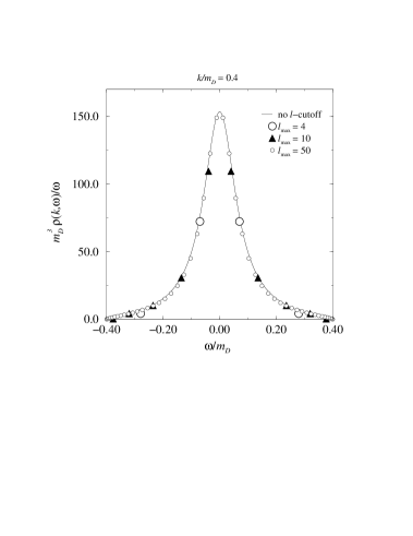
Figure 2: The spectral density $\rho/\omega$ at $k=0.4m_{\rm D}$ for propagators without the $l$-cutoff and with various values of $l_{\rm max}$. The spectral density for finite $l_{\rm max}$ is a sum of form $\sum_{\alpha}C_{\alpha}\delta(\omega-\omega_{\alpha})$. The plot symbols are plotted at coordinates $(\omega_{\alpha},2C_{\alpha}/(\omega_{\alpha+1}-\omega_{\alpha-1}))$, which makes it possible to compare the different $l_{\rm max}$-values.

The spectral power density

$$\rho(\omega,{\bf k})/\omega=(2/\omega)\mbox{\,Im\,}\Delta(\omega+i\epsilon,{\bf k})$$ (4.19)

for fixed $k=0.4m_{\rm D}$ is plotted in Fig. 2, both for the full propagator without the $l$-cutoff and for several (even) values of $l_{\rm max}$. In the finite $l_{\rm max}$ case the spectral density gets contributions only from the poles of the propagator (4.12):

$$\rho_{l_{\rm max}}(\omega,k)/\omega=\sum_{\rm poles}-{\frac{2\pi}{\omega}}\delta(\omega-\omega_{\rm pole}(k))\times\mbox{Res\,}\Delta_{l_{\rm max}}(\omega_{\rm pole}(k),k)\,.$$ (4.20)

The spectral power is strongly concentrated around $\omega=0$ with a peak width $\delta\omega\approx 4k^{3}/(\pi m_{\rm D}^{2})$. The spectral power of the $l_{\rm max}$ propagator closely follows the $l_{\rm max}=\infty$ curve; however, in order to have enough power in the central peak region, $l_{\rm max}$ should be large enough so that there are poles well within the bulk of the peak, which is the relevant region for the propagator to describe the correct damping.

We can use this property to derive an approximate ‘rule-of-thumb’, which tells how large $l_{\rm max}$ should be for a given value of $k$ (which, for the relevant physics, should be set to $g^{2}T$): we simply require that $l_{\rm max}$ is large enough so that lowest positive frequency pole satisfies

$$\omega_{\rm pole}(k)<{\frac{4k^{3}}{\pi m_{\rm D}^{2}}}\,.$$ (4.21)

Numerically, this corresponds to

$$l_{\rm max}^{\rm even}>0.62m_{\rm D}^{2}/k^{2}-0.8,\hskip 11.38109pt\hskip 11.38109ptl_{\rm max}^{\rm odd}>1.86m_{\rm D}^{2}/k^{2}-1.1\,,$$ (4.22)

with good accuracy. Strikingly, one has to use 3 times larger values for $l_{\rm max}$ in the odd sector than in the even one. This is due to the lack of the $\omega\sim k^{2}$ -pole in the odd sector, as emphasized above. While for modest values of $g^{2}T/m_{\rm D}=0.3\ldots 0.5$, $l_{\rm max}=6$ or 4 should be sufficient, for very weak coupling or large $m_{\rm D}$ the required $l_{\rm max}$-value becomes impractical for numerical work, since the numerical effort will rise as $(l_{\rm max}+1)^{2}$.

Naturally, one has to remember that Eq. (4.22) is based on an ad hoc requirement that the lowest positive frequency pole should be within the peak of the spectral density, and different criteria would lead to very different requirements (but the overall pattern in Eq. (4.22) should remain). What value of $l_{\rm max}$ one really needs in non-abelian simulations may differ from Eq. (4.22) by a large factor; indeed, the numerical results for non-abelian theory in Sect. 7 seem to imply that Eq. (4.22) is overly strict.

We also note that the poles of the $W$ field coincide with the $A$ field poles, so we have gotten them for free. For odd $l_{\rm max}$, there is one pole not accounted for yet: the mode corresponding to the $C_{ll^{\prime}}$ zero eigenvalue, which does not propagate at all. Naturally, the spectral power of the $W$ propagator is very different from the $A$ propagator.

So, what do these results tell us about the sphaleron rate in the non-abelian theory? We conclude the following:

A. When $l_{\rm max}$ is odd, a component of the gauge field is static and not fluctuating, and therefore does not contribute to real time processes. Since the static component is largest in the infrared, we expect this to reduce $\Gamma$ relative to large $l_{\rm max}$ limit. This behavior is worse for small $l_{\rm max}$ and should go away at large $l_{\rm max}$ as the static component contains less and less of the total gauge field amplitude.

B. In the even $l_{\rm max}$ sector, the location and density of the poles is relevant for the correct damping  in hot plasma: the larger $l_{\rm max}$ is, the more the poles are able to reproduce the concentration of spectral power at small $\omega$, and so the stronger the damping and the smaller the sphaleron rate. Thus, when $l_{\rm max}$ increases, the sphaleron rate should approach the physical one from above. The approach should be much faster than in the odd $l_{\rm max}$ sector, see Eq. (4.22).

This behavior is indeed close to what we observe in Sect. 7.

Obviously, the results in this section imply that for fixed $l_{\rm max}$ one cannot  have the correct leading order (in $g$) behavior of the gauge field propagator in the strict small $g$ limit. We expect this to be true also for the non-abelian gauge propagator, and hence for the sphaleron rate. Nevertheless, for realistic values of $g$ and $m_{\rm D}$ we expect a modest $l_{\rm max}$ to be sufficient.

5 Lattice equations of motion

In this section we discuss the discretization of the continuum equations of motion Eqs. (2.3), (3.4) and (3.7). Naturally, not all of the properties of the continuum evolution can be satisfied on a discrete lattice, but the update rule of the lattice system should fulfill at least the following criteria:

(i) Gauge invariance, lattice translational and rotational symmetry and C, P, and T symmetries are preserved,

(ii) Gauss’ law is identically satisfied,

(iii) The total energy is conserved.

Naturally, we also require that the small lattice spacing and smooth field limit gives the correct continuum behavior.

The discretization of the system is very similar to the pure Yang-Mills theory, developed by Kogut and Susskind [33]. The lattice is a 3-dimensional torus of size $L^{3}=N^{3}\,a^{3}$, with lattice spacing $a$. As is customary in real-time simulations, we use $A_{0}=0$ gauge and discretize the gauge fields in terms of spatial parallel transporters $U_{i}(x)=\exp(igaA_{i})\in\mbox{SU(2)}$, and electric fields $E_{i}(x)$ which belong to the Lie algebra of SU(2). $U_{i}(x)$ and $E_{i}(x)$ live on the links connecting points $x$ and $x+i$ (here we use the shorthand $x+i$ for $x+a\hat{e}_{i}$). The $W_{lm}$ fields are located on lattice sites. Thus, for each lattice site the total number of field variables is 3 SU(2)-matrices and $3+(l_{\rm max}+1)^{2}$ adjoint matrices.

On the lattice we want to use dimensionless field variables. We absorb the lattice spacing and $g$ in lattice fields as follows:

$$gaA\rightarrow A\,,\hskip 11.38109pt\hskip 11.38109ptga^{2}E\rightarrow E\,,\hskip 11.38109pt\hskip 11.38109ptgaW\rightarrow W\,.$$ (5.1)

For compactness, we also use dimensionless lattice coordinates, $x_{i}\rightarrow x_{i}a$, $x_{i}$ integer, reintroducing $a$ when necessary. We shall consider the evolution of the lattice fields both in continuous and discrete time. In discrete time, one update step consists of evolving the fields from time $t$ to $t+\delta_{t}$, where $\delta_{t}\ll 1$ in order to keep the evolution stable and integration errors small.

5.1 Gauge field update

We shall use the standard single plaquette definition for the magnetic field strength:

$${\frac{1}{T}}\int d^{3}x{\frac{1}{4}}F_{ij}^{a}F_{ij}^{a}\rightarrow\beta_{\rm L}\sum_{\Box}\big{[}1-{\textstyle{\frac{1}{2}}}{\rm Tr\,}U_{\Box}\big{]}\,.$$ (5.2)

Here $U_{\Box}$ is the ordered product of the link variables around a plaquette,

$$U_{\Box,ij}(x)=U_{i}(x)U_{j}(x+i)U^{\dagger}_{i}(x+j)U^{\dagger}_{j}(x)\,,$$ (5.3)

At tree level $\beta_{\rm L}=4/(g^{2}Ta)$. However, this receives radiative corrections; these will be discussed below.

Let us now consider the lattice gauge field equations of motion both in continuous and discrete time. The (continuous) time derivative of the link matrix $U$ is given in terms of the electric field as

$$\partial_{t}U_{i}(x,t)=iE_{i}(x,t)U_{i}(x,t)\,.$$ (5.4)

The ‘gauge force’ term in the evolution equation of the electric field is fixed by the magnetic Hamiltonian (5.2), by varying Eq. (5.2) with respect to $A_{i}$. When we add the current term due to the $W_{lm}$ fields, we obtain the evolution equation for $E_{i}$:

$$\partial_{t}E^{a}_{i}(x,t)=-i{\textstyle{\frac{1}{2}}}{\rm Tr\,}\bigg{[}\tau^{a}U_{i}(x,t)\sum_{|j|\neq i}S^{\dagger}_{ij}(x,t)\bigg{]}+{\frac{1}{2}}\big{[}j^{a}_{i}(x,t)+{\cal P}^{ab}_{i}j^{b}_{i}(x+i,t)\big{]}\,.$$ (5.5)

Here $S_{ij}$ is the gauge link ‘staple’ which connects the points $x$ and $x+i$ around the plaquette:

$$S_{ij}=U_{j}(x)U_{i}(x+j)U^{\dagger}_{j}(x+i)$$ (5.6)

The summation index $j$ in Eq. (5.9) goes over both positive and negative directions; a negative value means that the link is traversed in the opposite direction as in Eq. (5.6): $U_{-j}(x)=U_{j}^{\dagger}(x-j)$.

The current terms in Eq. (5.5) are given by $j^{a}_{i}=(m_{\rm D}a)^{2}/(4\pi)v^{*}_{mi}W^{a}_{1m}$. Since $E_{i}(x)$ is located between the points $x$ and $x+i$, the current $j_{i}(x)$ is averaged between the beginning and the end of the link. The current at $x+i$ has to be parallel transported to point $x$, and we use the shorthand expression

$${\cal P}^{ab}_{i}\Phi^{b}(x+i,t)=[U_{i}(x,t)\Phi(x+i,t)U^{\dagger}_{i}(x,t)]^{a}$$ (5.7)

for the adjoint field parallel transport from point $x+i$ to point $x$.

In discrete time, the adjoint field $E_{i}$ transports the link matrix $U_{i}(t)$ to $U_{i}(t+\delta_{t})$. In order to keep the evolution symmetric in time, it is natural to place $E_{i}$ in the half-timestep value $t+{\textstyle{\frac{1}{2}}}\delta_{t}$. Integrating Eq. (5.4), we obtain the discrete time evolution equation for $U_{i}$:

$$U_{i}(x,t+\delta_{t})=\exp\big{[}iE_{i}(x,t+{\textstyle{\frac{1}{2}}}\delta_{t})\,\delta_{t}\big{]}\,U_{i}(x,t)\,.$$ (5.8)

Alternatively, one can think of $\exp(iE_{i}\delta_{t})$ as being the timelike plaquette in the $(t,i)$ plane, which updates $U$ as shown because we have chosen $A_{0}=0$ gauge. (In another gauge there would be an extra $A_{0}$ dependent term in the $U$ field update, and in the updates of the $E$ and $W$ fields as well; it is the convenience of leaving these out which encourages the choice of temporal gauge.)

The discrete time electric field update can be obtained now from Eq. (5.5) by substituting

$$\partial_{t}E^{a}_{i}(x,t)\rightarrow{\frac{1}{\delta_{t}}}[E^{a}_{i}(x,t+{\textstyle{\frac{1}{2}}}\delta_{t})-E^{a}_{i}(x,t-{\textstyle{\frac{1}{2}}}\delta_{t})]\,.$$ (5.9)

The lhs of Eq. (5.5) remains as is even at discrete time. As formulated, the discrete time update steps (5.8) and (5.9) are symmetric under time reversal and they give an algorithm accurate to order $O(\delta_{t}^{2})$.

As mentioned above, the relation $\beta_{\rm L}=4/(g^{2}Ta)$ receives corrections because UV modes behave differently on the lattice than in the continuum. This has been calculated in Appendix B of [24] (see also [34]), with the result

$$\beta_{\rm L} = {\frac{4}{g^{2}aT}}+\left(\frac{1}{3}+\frac{37\xi}{6\pi}\right)-\left(\frac{4}{3}+\frac{2m^{2}_{D}a^{2}}{3}+\frac{m^{4}_{D}a^{4}}{18}\right)\frac{\xi(m_{\rm D}a)}{4\pi}$$ (5.10)

$${}+\left(\frac{1}{3}+\frac{m^{2}_{D}a^{2}}{18}\right)\frac{\Sigma(m_{\rm D}a)}{4\pi}\,.$$

Here $\xi=0.152859\ldots$, and $\Sigma(m_{\rm D}a)$ and $\xi(m_{\rm D}a)$ are integral functions:

$$\Sigma(m)=\int_{-\pi}^{\pi}{\frac{d^{3}k}{(2\pi)^{3}}}{\frac{1}{\hat{k}^{2}+m^{2}}}\,,\hskip 11.38109pt\hskip 11.38109pt\hskip 11.38109pt\xi(m)=\int_{-\pi}^{\pi}{\frac{d^{3}k}{(2\pi)^{3}}}{\frac{1}{(\hat{k}^{2}+m^{2})^{2}}}\,,$$ (5.11)

where $\hat{k}^{2}=\sum_{i}4\sin^{2}k_{i}/2$. To 5% accuracy, this can be expressed as $\beta_{\rm L}\simeq 4/(g^{2}aT)+0.61$ for values of $m_{\rm D}a$ used in this work. However, we shall use the full expression in our analysis. In the sequel we will write $\beta_{L}$ for the variable appearing in Eq. (5.10), and write $\beta$ for $4/g^{2}aT$.

Further subtleties related to this thermodynamic correction arise when we convert $\Gamma$ to continuum limits; we will address this in Appendix C.

5.2 $W_{lm}$ update and doublers

The $W_{lm}$ equation of motion Eq. (3.4) has only first order derivatives in time and space. In order to preserve the exact $P$ and $T$ symmetries on the lattice, the first order derivative terms should be replaced by symmetric  finite differences. Thus, the continuous time lattice equation of motion for $W_{lm}$ is

$$\partial_{t}W_{lm}(x,t) = -{\frac{1}{2}}\,C_{lm,l^{\prime}m^{\prime},i}[{\cal P}_{i}W_{l^{\prime}m^{\prime}}(x+i,t)-{\cal P}_{-i}W_{l^{\prime}m^{\prime}}(x-i,t)]$$ (5.12)

$$+ {\frac{1}{2}}\delta_{l,1}v_{mi}[E_{i}(x,t)+{\cal P}_{-i}E_{i}(x-i,t)]\,.$$

The electric field contribution is symmetrized from each of the links which connect to point $x$.

As was done with the spatial derivative, we substitute the time derivative $\partial_{t}W$ with a symmetric finite difference $[W(t+\delta_{t})-W(t-\delta_{t})]/(2\delta_{t})$, and the value of $W$ at time $t+\delta_{t}$ will depend on values at times $t$ and $t-\delta_{t}$. Explicitely, the update rule becomes a ‘leapfrog’

$$W_{lm}(x,t+\delta_{t}) = W_{lm}(x,t-\delta_{t})+\delta_{t}\bigg{\{}2\delta_{l,1}v_{mi}E_{{\rm ave},i}$$ (5.13)

$$- C_{lm,l^{\prime}m^{\prime},i}[{\cal P}_{i}W_{l^{\prime}m^{\prime}}(x+i,t)-{\cal P}_{-i}W_{l^{\prime}m^{\prime}}(x-i,t)]\bigg{\}}\,.$$

Here $E_{\rm ave}$ is the average electric field influencing the propagation of $W_{lm}$ from $t-\delta_{t}$ to $t+\delta_{t}$. Since this is over two timesteps, there are 4 timelike ‘plaquettes’ to each direction $i$:

$$E_{{\rm ave},i}(x,t) = {\frac{1}{4}}[E_{i}(x,t-{\textstyle{\frac{1}{2}}}\delta_{t})+{\cal P}_{-i}E_{i}(x-i,t-{\textstyle{\frac{1}{2}}}\delta_{t})$$ (5.14)

$$~{}{}+E_{i}(x,t+{\textstyle{\frac{1}{2}}}\delta_{t})+{\cal P}_{-i}E_{i}(x-i,t+{\textstyle{\frac{1}{2}}}\delta_{t})]\,.$$

Note that, due to Eq. (5.8), the parallel transport ${\cal P}_{-i}E_{i}(x,t+{\textstyle{\frac{1}{2}}}\delta_{t})$ can be made with $U$ matrices either at time $t$ or time $t+\delta_{t}$ with the same result. In practice, one does the $E_{i}$ transport once for each timestep, and stores the result for the next timestep.

To summarize, the discrete time update step ($t\rightarrow t+\delta_{t}$) goes as follows:

• start with $U(t)$, $E(t-\delta_{t}/2)$, $W(t)$ and $W(t-\delta_{t})$,

• evaluate $E(t+\delta_{t}/2)$ with Eqs. (5.9) and (5.5),

• calculate $W(t+\delta_{t})$ with Eq. (5.13) (and forget $W(t-\delta_{t})$ and $E(t-\delta_{t}/2)$), and finally

• calculate $U(t+\delta_{t})$ with Eq. (5.8).

A generic feature of a first order differential operator on a discrete lattice is the decoupling of ‘odd’ and ‘even’ coordinate sectors: $W_{lm}(x,t+\delta_{t})$ depends only on $W_{lm}$ at points $(x,t-\delta_{t})$ and $(x\pm i,\delta_{t})$; in particular it does not  depend on $W_{lm}(x,t)$, which is its immediate predecessor. More precisely, if we label the coordinates with an integer valued parity label $p=\sum_{i}x_{i}+t/\delta_{t}$, the $W_{lm}$ fields at odd and even values of $p$ do not interact, except through their coupling to the gauge fields. This causes a species doubling problem, in analogy to the one familiar from lattice QCD (the Dirac equation is of first order). The properties of the doublers in a linearized theory are discussed in detail in Appendix B.

There are 15 extra low-energy doubler modes, living around the corners of the 4-momentum space hypercube $k_{i}=(0,\pi/a)$, $\omega=(0,\pi/(\delta_{t}a))$, with at least one of $k_{i},\,\omega$ non-zero. The continuous time equation of motion $(\ref{dW})$ has only 7 spatial doublers; the rest are introduced by the time discretization (and can be avoided, see subsection 5.4). However, in contrast to lattice QCD, in our case the doublers are benign: first, they couple only very weakly to the gauge fields, decoupling completely at the corners of the Brillouin zone (see Appendix B). Second, they couple only to gauge fields at very high wave numbers $k\sim 1/a$ and/or frequencies $\omega\sim 1/(a\delta_{t})$. Thus, the doublers do not influence at all the physically interesting small $k$ and $\omega$ gauge field dynamics, and their effect on modes close to the lattice cutoff remains small.

Because the time step is small ($\delta_{t}\ll 1$), the timelike doubler modes $\omega\sim\pi/a\delta_{t}$ are especially weakly coupled to low-frequency modes. Indeed, in simulations we used $\delta_{t}=0.05$ and observed no appreciable energy transfer between the timelike doublers and low-frequency modes. However, since the timelike doublers are low-energy excitations of $W$ fields which are not present in continuous time, they can cause problems in thermalization of the system and, as it turns out, in counting the active degrees of freedom. This will be discussed below in section 5.6.

Before leaving the update we should comment on energy conservation. In continuous time, we can write down the lattice version of the Hamiltonian (3.8):

$$H(t)=\beta_{\rm L}\sum_{\Box}\big{[}1-{\textstyle{\frac{1}{2}}}{\rm Tr\,}U_{\Box}(t)\big{]}+{\frac{1}{2}}\sum_{x,i}E_{i}^{2}(x,t)+{\frac{(m_{\rm D}a)^{2}}{8\pi}}\sum_{x,lm}|W_{lm}(x,t)|^{2}\,.$$ (5.15)

This Hamiltonian is exactly conserved by the equations of motion (5.4), (5.5) and (5.12). However, in discrete time there is no equivalent conserved expression. A good approximation to the energy can be obtained by symmetrizing the contribution of the electric fields in Eq. (5.15) with respect to $t$:

$$E_{i}^{2}(x,t)\rightarrow[E_{i}^{2}(x,t-{\textstyle{\frac{1}{2}}}\delta_{t})+E_{i}^{2}(x,t+{\textstyle{\frac{1}{2}}}\delta_{t})]/2\,.$$ (5.16)

The energy obtained this way fluctuates with an amplitude $\propto\delta_{t}^{2}$, but the mean value is stable. The conservation of mean energy is guaranteed by the time reversal symmetry of the discrete time equations of motion: if, at some point in the evolution of the fields, we invert the sign of $E$ ($E\rightarrow-E$) and conjugate and reverse sign for the hard particle charges ($W_{lm}\rightarrow-W^{*}_{lm}=-(-1)^{l}W_{lm}$), the system will exactly retrace its evolution backwards. If the energy had a tendency to increase, inverting the time would cause it to decrease. Since the configurations $(U,E,W)$ and $(U,-E,-W^{*})$ are just as likely to appear in a thermal distribution, the system cannot exhibit any systematic tendency for the average energy to change. The stability of the system is a necessary property for long Hamiltonian evolutions.

5.3 Gauss’ constraint

The Gauss’ law is given by the 0-component of the equations of the motion (2.3):

$$D_{i}F^{i\,0}=j^{0}={\frac{m_{\rm D}^{2}}{\sqrt{4\pi}}}W_{00}\,.$$ (5.17)

On the discrete spatial lattice and discrete time, care has to be taken to make the appropriate symmetrizations to the fields $F_{i0}=E_{i}$ and $W$ appearing in Eq. (5.17). Since $E_{i}$ is living on half timestep time values $t+{\textstyle{\frac{1}{2}}}\delta_{t}$, we symmetrize $W_{00}$ from times $t$ and $t+\delta_{t}$:

$$\sum_{i}\bigg{[}E_{i}(x,t+{\textstyle{\frac{1}{2}}}\delta_{t})-{\cal P}_{-i}E_{i}(x-i,t+{\textstyle{\frac{1}{2}}}\delta_{t})\bigg{]}$$

$$\hskip 11.38109pt{}+{\frac{(m_{\rm D}a)^{2}}{\sqrt{4\pi}}}{\frac{1}{2}}[W_{00}(x,t)+W_{00}(x,t+\delta_{t})]=0$$ (5.18)

This condition (or rather, the constancy of the violation of this condition) is satisfied exactly by the evolution equations (5.8), (5.9) and (5.13). To see this consider the change of Eq. (5.18) under one time step. It gets contributions from each $dE/dt$ and from $dW_{00}/dt$. (There are no contributions from the time derivative $dU/dt$ of the $U$ appearing in the parallel transporter ${\cal P}_{-i}$ because $dU/dt$ commutes with $E$ and cancels between the $U$ and $U^{\dagger}$ in Eq. (5.7).) In the absence of $W$ fields, the time derivative of Eq. (5.18) is zero, as shown by Ambjørn and Krasnitz [10]. The addition of $W$ fields adds new terms to the $W_{00}$ field and $E$ field updates. First there is a contribution to $E_{i}(x)$ and ${\cal P}_{-i}E_{i}(x-i)$ from $W_{1m}(x)$. According to Eq. (5.5) these are equal; but $E_{i}(x)$ and ${\cal P}{-i}E_{i}(x-i)$ appear in Eq. (5.18) with opposite sign, so there is no contribution here. There is also no contribution to $dW_{00}(x)/dt$ due to $W_{1m}(x)$. Second, $W_{1m}$ at each neighboring site contributes both to $dE/dt$ on the link between the neighboring site and $x$, and to $dW_{00}/dt$, through Eqs. (5.9) and (5.13) respectively; but the two contributions to the time derivative of Eq. (5.18) cancel, because $C_{00,1m,i}=v^{*}_{mi}$. Hence the update preserves Gauss’ law if it is satisfied by the initial conditions. Enforcement of Gauss’ law is therefore a problem for the thermalization algorithm, not the evolution.

5.4 A way to eliminate temporal doublers

There is an alternative way to write the update rules which eliminates all the high frequency doubler modes, which we now discuss. First, note that the reason there are doublers is that the update as specified in the previous subsections requires and maintains twice as much information about the $W$ fields as is necessary. As discussed in the summary at the end of subsection 5.2, the update needs the value of $W_{lm}$ at two time slices. However, only $W$ and not its time derivative appear in the Hamiltonian, so a complete specification of the fields should only require $W_{lm}$ to be specified once at each site. The excess information describes the state of the doublers. Eliminating the doublers will require eliminating half of this information. This is possible since, as noted earlier, the update rule for $W$ does not mix the $W$ fields on odd and even sublattices. Therefore, it is possible to define $W$ only at every other spacetime point; we can define it only at the even sites, that is, points for which $p=\left[t/\delta_{t}+\sum_{i}x_{i}\right]$ is even. Eq. (5.14) remains unchanged, but Eq. (5.9) has the modification

$$\big{[}j^{a}_{i}(x,t)+{\cal P}^{ab}_{i}j^{b}_{i}(x+i,t)\big{]}\rightarrow\left\{\begin{array}[]{cc}j_{i}^{a}(x,t)\;,&\quad t/\delta_{t}+\sum_{i}x_{i}\;{\rm even}\\ &\\ {\cal P}_{i}^{ab}j_{i}^{b}(x+i,t)\;,&\quad t/\delta_{t}+\sum_{i}x_{i}\;{\rm odd}\\ \end{array}\right.\,,$$ (5.19)

that is, we use whichever $j$ is defined. Similarly, in Gauss’ law, Eq. (5.18) involves either $W_{00}(x,t)$ or $W_{00}(x,t+\delta_{t})$, whichever is defined. The time derivative of the Gauss constraint remains conserved, for the same reasons as before.

Updating the fields in this way removes 8 of the 15 doublers and cuts the number of computations, and hence the CPU time, almost in half. It may slightly increase timestep errors because of the even-odd alternation of the current in the $E$ field update rule; but this can be compensated for by reducing $\delta_{t}$, which is not problematic because of the reduction in the number of computations per time step. We have compared the update with and without this modification and find that the results for physical measurables agree within statistical errors.

5.5 Lattice thermodynamics

In continuous time the equations of motion (5.4), (5.5), and (5.12) describe a Hamiltonian evolution which conserves energy and phase space volume. We can study the thermodynamics of the system by using the Hamiltonian (5.15) to write down the canonical partition function

$$Z=\int\bigg{[}\prod_{x,i}dU_{i}(x)dE_{i}(x)\bigg{]}\bigg{[}\prod_{x,lm}dW_{lm}(x)\bigg{]}\prod_{x}\delta(G(x))\,e^{-H/T}\,,$$ (5.20)

where $G(x)$ is Gauss’ law, Eq. (5.18) (in continuous time). Introducing a Lagrange multiplier field $A_{0}$ in exact analogy with what we did in continuous space in subsection 4.1, we can integrate out the $E$ and $W$ fields to obtain the lattice partition function

$$Z = \int\bigg{[}\prod_{x,i}dU_{i}(x)\bigg{]}\bigg{[}\prod_{x}dA_{0}(x)\bigg{]}e^{-H_{A}}\,,$$ (5.21)

$$H_{A} = \beta_{\rm L}\sum_{\Box}\big{[}1-{\textstyle{\frac{1}{2}}}{\rm Tr\,}U_{\Box}(t)\big{]}+$$ (5.22)

$${\frac{1}{2}}\sum_{x,i}[{\cal P}_{i}A^{a}_{0}(x+i)-A^{a}_{0}(x)]^{2}+{\frac{(m_{\rm D}a)^{2}}{2}}\sum_{x}(A^{a}_{0}(x))^{2}\,.$$

The gradient term for the $A_{0}$ field is the simplest lattice implementation of the continuum $(D_{i}A_{0})^{2}$, and $m_{\rm D}^{2}$ appears as the $A_{0}$ mass term without any corrections, just as in the continuum case. The form of the partition function above is equivalent to the path integral of the full quantum theory in the high-temperature dimensional reduction approximation on the lattice [35, 36]. This guarantees that this theory reproduces the (equal time) thermodynamics of the Yang-Mills fields.

This property can be used to fix the bare lattice value of the mass term $m_{\rm D}$. In general, classical field theories suffer from UV divergences; however, when we consider the static thermodynamics of the theory in Eq. (5.22), only a finite number of UV divergent diagrams appears. These divergences can be absorbed in counterterms, and in particular for the theory in Eq. (5.22), we have [35]

$$m^{2}_{\rm D,bare}=m^{2}_{\rm D,phys}-{\frac{\Sigma g^{2}T}{\pi a}},\hskip 11.38109pt\hskip 11.38109pt\Sigma=3.17591\ldots\,.$$ (5.23)

Here $m^{2}_{\rm D,phys}$ is fixed according to the actual particle content of the theory, see Eq. (2.9).

5.6 Thermalization

The real time simulation has to be started from a configuration which has been chosen from a thermal distribution so that the the Gauss’ constraint is satisfied. As emphasized above, to start the update we need the fields $U(t)$, $E(t-\delta_{t}/2)$, $W(t)$ and $W(t-\delta_{t})$.

We will use the same general philosophy as in [11]. Some of the degrees of freedom, namely $E_{i}$ and $W_{lm}$, are Gaussian, while others, namely $U_{i}$, are not. We can draw the Gaussian fields from the thermal ensemble and then use the evolution equations to “mix” this thermalization with those degrees of freedom which are not Gaussian. The thermalization proceeds by evolving the Hamiltonian equations of motion of the system, but periodically “refreshing” the Gaussian degrees of freedom, that is, discarding the values of Gaussian degrees of freedom and drawing them from the thermal ensemble.

At first sight, this plan appears to be complicated due to the Gauss’ constraint. In the case without the $W$ fields this problem was solved in [11], by first drawing $E$ from the Gaussian distribution ignoring the constraint and then projecting to the constraint surface. It is trivial to extend that technique to the current situation. However it is actually possible to do something even easier. Only the component $W_{00}$ of $W_{lm}$ enters the Gauss’ constraint. Thus, according to Eq. (5.15), we can set the higher $lm$-components freely to the correct thermal distribution, that is, draw each of $W_{lm}^{a}$, $l\geq 1$, from a Gaussian distribution of width $\sqrt{8\pi/(m_{\rm D}a)^{2}}$. The thermalization then proceeds as follows:

• Set $U(x,t)=1$, $E(x,t)=W_{00}(x,t)=0$.

• Choose $W^{a}_{lm}(x,t)$, $l\geq 1$, from the Gaussian distribution of width $\sqrt{8\pi/(m_{\rm D}a)^{2}}$.

• Evolve the equations of motion for a short period, transferring energy from $W_{lm}$ to the other fields, while preserving Gauss’ law.

• Repeat from (2) until the fields are thermalized.

However, in discrete time we do not have an exact Hamiltonian, and there is an inherent ambiguity $\propto\delta_{t}^{2}$ in the definition of energy. It is not immediately evident how the fields should be thermalized. At a more practical level, the randomization of $W_{lm}$ as above is complicated by the fact that we need $W_{lm}$ fields at times $t$ and $t-\delta_{t}$ to start the leapfrog update. This is closely associated with the timelike doublers of the $W$ fields. However, as was discussed in section 5.2, the timelike doublers couple extremely weakly to the low-frequency mode sector, and there is practically no energy transfer between the two sectors. This was also seen in simulations: the energy contained in the doubler modes remained at the level where it was set by the initial thermalization during the whole trajectory. Moreover, the gauge fields care only about the low frequency modes (see Appendix B). Thus, in principle, we are at liberty to do whatever we choose about the timelike doubler modes; we can either thermalize them or try not to excite them in thermalization. The gauge fields will not see the difference — however, in the former case $W$ fields will contain roughly twice as much energy as in the latter. Note also that the whole problem would go away if we used the update discussed in subsection 5.4.

In all of our ‘production’ runs we chose not to excite the timelike doubler modes. This makes the lattice modes resemble as closely as possible the continuous time fields. Note that the Hamiltonian (5.15) counts the degrees of freedom and energy equipartition correctly only if there are no timelike doublers, and the $O(\delta_{t}^{2})$ ambiguity in energy is valid only in this case (in the presence of doublers, the ambiguity is of order 100%).

The thermalization without the doublers can be accomplished using the steps (1)–(4) as above, but replacing the step (2), for example, by one of the following two methods:

(a) Set $W_{lm}(t)$ to Gaussian random variables in step (2) above, and perform the first update step in (3) using a forward asymmetric time difference for these $lm$ modes: that is, instead of approximating the time derivative with $[W(t+\delta_{t})-W(t-\delta_{t})]/(2\delta_{t})$ in Eq. (5.13), we use $[W(t+\delta_{t})-W(t)]/\delta_{t}$. This is a natural way to start a leapfrog, and it gives a smooth interpolation for the fields. This method gives slightly incorrect mean energy, but the error is $O(\delta_{t}^{2})$.

(b) Set $W_{lm}(x,t-\delta_{t})=W_{lm}(x,t)$, where $l\geq 2$, to Gaussian random variables in step (2). Now also the first step can be performed with the leapfrog. This method excites the doublers more, but the amplitude of their excitation is only $O(\delta_{t}^{2})$. Note that now only modes $l\geq 2$ can be randomized, since in one timestep both $E$ and $W_{00}$ interact with with $l=0$ modes.

In our production runs we used the method (b). We also made test runs with the doubler modes fully exited. This is simple to accomplish: proceed as in items (1)–(4) above, randomizing only $W_{lm}(t)$, $l\geq 2$, and perform the evolution with the leapfrog update (5.13). Since there are now twice as many active $W_{lm}$ modes, the width of the Gaussian distribution has to be multiplied by $\sqrt{2}$, in order for the $U$ and $E$ fields to have the same total energy as before. As mentioned above, in the gauge field observables the doublers have no observable effect.

Let us note that a Langevin-type thermalization, as used in [37] for pure Yang-Mills theory, would be straightforward to implement by coupling the noise to $W_{lm}$ fields. Indeed, coupling the noise only to the highest $l$-modes might be of interest even during a simulation, since this could mimic the effect of the higher $l$ modes.

6 Measuring the Chern-Simons number diffusion

The baryon number violation rate is related to the diffusion of the Chern-Simons number, defined as the charge associated with the right-hand side of the anomaly equation (1.1):

$$N_{\rm CS}={\frac{g^{2}}{32\pi^{2}}}\int d^{3}x\epsilon_{ijk}\left(F_{ij}^{a}A_{k}^{a}-\frac{1}{3}f_{abc}A^{a}_{i}A^{b}_{j}A^{c}_{k}\right)={\frac{1}{N_{G}}}\int d^{3}xJ_{B}^{0}\,.$$ (6.1)

Since SU(2) has a non-trivial third homotopy group $\pi_{3}(\mbox{SU(2)})={\bf Z}$ the Chern-Simons number $N_{\rm CS}$ is a topological index for vacuum configurations: we can perform any gauge transformation to a trivial configuration $A=0$ without any cost in energy, and the resulting configuration is as good a vacuum configuration as the initial one. $N_{\rm CS}$ is equal to the winding number of this gauge transformation. Since it is now integer valued, it classifies the vacuum configurations into disconnected classes, which cannot be continuously gauge transformed to each other. Thus, a vacuum-to-vacuum process which increases $N_{\rm CS}$ smoothly by one unit must go through a non-vacuum exited state, the sphaleron. Due to the axial coupling to fermionic current, this process lifts one left-handed solution of the Dirac operator from negative to positive energy, and pushes one right handed state from positive to negative energy. Since the SU(2) sector of the standard model is a chiral theory which does not couple to the right-handed fermions, this process will create one fermion for each fermionic generation ($N_{G}$).

At high temperatures the Chern-Simons number diffuses readily, and integer values are not particularly preferred. In any given volume the Chern-Simons number performs a random walk in time, and the diffusion constant, $\Gamma$, can be measured from

$$\Gamma=\lim_{V\rightarrow\infty}\lim_{t\rightarrow\infty}{\frac{\langle(N_{\rm CS}(t)-N_{\rm CS}(0))^{2}\rangle}{Vt}}\,.$$ (6.2)

Here the angle brackets $\langle\cdot\rangle$ refer to an average over the thermal ensemble. The change in the Chern-Simons number can be evaluated from

$$N_{\rm CS}(t)-N_{\rm CS}(t_{0})={\frac{g^{2}}{8\pi^{2}}}\int_{t_{0}}^{t}dt^{\prime}\int d^{3}xE_{i}^{a}B_{i}^{a}\,.$$ (6.3)

In principle, this measurement is readily convertible to lattice language: lattice versions of the fields $E$ and $B$ feature prominently in the equations of motion (5.4),(5.5). However, this “naive” definition of $N_{\rm CS}$ on the lattice, often used in the early work on Chern-Simons number diffusion in lattice SU(2) gauge theory [9, 10, 11, 12], suffers from spurious noise and diffusion which obscures the physical $N_{\rm CS}$ diffusion. Moreover, due to its UV nature, the amplitude of the noise diverges as $1/a$ in fixed physical volume, which is disastrous in the continuum limit. The reason for this noise is well understood: the integral over lattice $\bf E\cdot B$ on the right-hand side of Eq. (6.3) does not form a total time derivative, and hence it depends on the path along which one connects the initial and final configurations in Eq. (6.3). In other words, it does not give us a topological measurement.

In general, topology of lattice fields is ambiguous, since the variables are always continuously connected to trivial ones. However, at fine enough lattice spacings (still easy to achieve in our simulations) almost every one of the plaquettes is very close to unity in a thermal ensemble; large plaquette values are exponentially suppressed. Perturbatively this means that the gauge fields are small, and for this subset of lattice fields topology can be unambiguously defined [38]. Physically, this means that the spatial size of the topology changing configurations, sphalerons, is large in lattice units. This will be true because the energy of sphaleron-like configurations increases linearly with inverse size. The Boltzmann suppression factor for small (lattice scale) sphalerons is enormous and they, in practice, never appear in simulations. The interplay between entropy and the Boltzmann factor sets the dominant sphaleron size to be $\sim g^{2}T$. For topology to be unambiguously defined, our lattice spacing must be considerably smaller than this.

Two successful methods for measuring topology in the current “real time” context have been recently developed. The first method uses an auxiliary “slave field” to track the winding number of the gauge [14]. It is a development of a method originally proposed by Woit [39], which is based on counting the winding numbers of singularities in the Coulomb gauge. In this work we use the second method, “calibrated cooling.” This method is based on the cooling method by Ambjørn and Krasnitz [13], and fully developed by Moore in [15]. The rest of this section will summarize this method.

The calibrated cooling method relies directly on the fact that the sphalerons are large and extend over several lattice units. Thus, we can get rid of most of the ultraviolet noise in the thermal configuration by applying a small amount of cooling  to the configuration: the resulting configurations are very smooth on lattice scales, but they still have the same topological content as the original configuration. After cooling the integral (6.3) can be performed with small errors. The accumulation of residual errors is prevented by periodically cooling all the way to a vacuum configuration: we know that the true vacuum-to-vacuum $\delta N_{\rm CS}=\mbox{integer}$, and any deviation is due to accumulated integration error, which can thus be “calibrated” away. This is schematically described in Fig. 3.

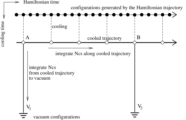
Figure 3: How the $N_{\rm CS}$ evolution is measured (after [15]). Top horizontal line shows the configurations (solid circles) generated by the lattice equations of motion. Every few timesteps, the configurations are cooled a fixed cooling length, giving a parallel cooled trajectory (open circles). Now the fields are smooth enough so that ${\bf E\cdot B}$ can be reliably integrated, giving $\delta N_{\rm CS}(t)$ along the cooled trajectory. In longer intervals, the $N_{\rm CS}$ measurement is “grounded” by cooling all the way to a vacuum configuration. If $\delta N_{\rm CS}$ along paths like $V_{1}\rightarrow A\rightarrow B\rightarrow V_{2}$ is always close to an integer, we know that the integration errors are small. The residual deviation from an integer value is subtracted from $\delta N_{\rm CS}(A\rightarrow B)$, cancelling the accumulation of errors.

The cooling path is defined by the gradient flow of the standard single plaquette Kogut-Susskind gauge action, given in Eq. (5.2). The evolution along this path is parametrized by fictitious cooling “time” $\tau$, dimensionally $\mbox{(length)}^{2}$. The cooling equation of motion is now [13]

$${\frac{\partial U_{i}(x)}{\partial\tau}}=i\sigma^{a}{\frac{\partial A^{a}_{i}}{\partial\tau}}U_{i}(x)=i\sigma^{a}{\textstyle{\frac{1}{2}}}{\rm Tr\,}\bigg{[}i\sigma^{a}U_{i}(x)\sum_{|j|\neq i}S^{\dagger}_{ij}(x)\bigg{]}U_{i}(x)\,.$$ (6.4)

Here the staple $S$ is defined as in Eq. (5.5). On the lattice the equation above is evolved in discrete $\tau$, and we use here optimized step lengths by alternating $\delta\tau/a^{2}=5/48$ and $10/48$. Too large a time step causes the UV modes to become unstable.

The evolution of (6.4) all the way to a vacuum configuration is a computationally demanding task, and it can easily dominate the cpu time. The integration can be dramatically accelerated by blocking  the lattice: after a bit of cooling the fields are very smooth at the lattice scale, and essentially no information is lost if we reduce the number of lattice points in each direction by a factor of 2. The blocked $U$-matrices are formed from the product of the matrices on the two links between the blocked points. Since the lattice spacing $a$ is now increased by a factor of 2, computational cost in cooling is reduced by a factor $2^{5}$ – a factor of 4 coming from the increase in the $\delta\tau$ step. In our calculations we block the configuration twice in the course of cooling to vacuum. For detailed information about this method we refer to [15].

In all of our simulations we cooled a configuration from the Hamiltonian trajectory at intervals $\delta t=0.5a$ (once in 10 timesteps with $\delta_{t}=0.05a$). We cooled to depth $\tau=a^{2}45/48$ for the cooled trajectory (see Fig. 3), using unblocked configurations. $\delta N_{\rm CS}$ was integrated along this trajectory using improved $O(a^{2})$ accurate definitions for ${\bf E\cdot B}$ [11]. The cooling to vacuum was performed with an interval $\delta t=12.5$. Our parameter choices were overly conservative: the vacuum-to-vacuum integration error was typically of order 0.02–0.04. Thus, it is possible to use much more aggressive optimization than we use here without losing the topological nature of this measurement (see ref. [18]).

7 Simulations and results

Our aim here is to answer the following questions:

• what is the dependence of the Chern-Simons number diffusion rate $\Gamma$ on the finite $l_{\rm max}$ cutoff, and is there an $l_{\rm max}$ which is ‘large enough’ for practical purposes or is an $l_{\rm max}\rightarrow\infty$ extrapolation necessary?

• is $\Gamma$, in physical units, independent of the lattice spacing?

• how does $\Gamma$ depend on the physical quantity $m_{\rm D}/g^{2}T$?

Let us first discuss the relation between the physical Debye mass $m_{\rm D}$ and the bare mass parameter $m_{\rm D}a$ on the lattice. As explained in Sect. 5.5, the bare mass receives renormalization counterterms and diverges in the UV limit as $1/a$. However, according to the scaling arguments of Arnold, Son and Yaffe [17], the sphaleron rate should not actually depend on the Debye mass, which characterizes static screening properties of the hot plasma, but on the damping rate of the transverse gauge field propagation. As explained in Sect. 4, this is related to the Debye mass in the continuum. However, due to the lattice dispersion relation, the hard gauge field modes do not propagate at the speed of light, and their effect on the damping is reduced. Averaging over all of the directions of the lattice momenta, Arnold [40] has calculated that the effect of the hard gauge field modes on the lattice is a factor of ($0.68\pm 0.2$) times smaller than the continuum relation between the damping coefficient and $m_{\rm D}^{2}$ would imply. The error quoted is systematic, and it takes into account the rotational non-invariance of the lattice propagators. Thus, we shall use the following relation between the bare lattice $m_{\rm D}$ and the continuum one:

$$Z^{-1}_{m_{D}}m_{D,\rm latt}^{2}=m_{D,\rm phys}^{2}-0.68{\frac{\Sigma g^{2}T}{\pi a}}\,.$$ (7.1)

Here $Z^{-1}_{m_{D}}$ is a radiative correction of form $1+O(a)$, see Eq. (C.14). We use the improved relation Eq. (5.10) to relate the lattice spacing $a$ to the physical scale $g^{2}T$. There are additional radiative corrections associated with renormalization of the lattice time scale, which we discuss in Appendix C. In order to avoid the uncertainties associated with the UV counterterm, we use mostly fairly large physical values of $m_{\rm D}$ so that the UV term remains subdominant. The results are actually quite robust against variations in the numerical coefficient 0.68, even with the smallest $m_{\rm D}$ we use.

run parameters $l_{\rm max}$ time$/a$ $\Gamma/(\alpha^{4}T^{4})$ $\beta_{\rm L}=8.7$, $V/a^{3}=24^{3}$ 0 8000 1.49(15) $m^{2}_{D}=1.59/a^{2}=8.20g^{4}T^{2}$ 1 20000 0.0606(70) 2 20000 0.531(34) 3 30000 0.345(23) 4 20000 0.520(22) 5 20000 0.445(30) 6 30000 0.534(27) 10 20000 0.518(34) $\beta_{\rm L}=12.7$, $V/a^{3}=32^{3}$ 2 37500 0.249(23) $m^{2}_{D}=1.98/a^{2}=20.7g^{4}T^{2}$ 4 37500 0.198(18) 6 45000 0.199(18) $\beta_{\rm L}=12.7$, $V/a^{3}=32^{3}$ 2 37500 0.839(36) $m^{2}_{D}=0.29/a^{2}=4.84g^{4}T^{2}$ 4 37500 0.687(50)

Table 1: How the sphaleron rate $\Gamma$ depends on $l_{\rm max}$.

$l_{\rm max}$ dependence:

In order to study how the sphaleron rate depends on the value of $l_{\rm max}$, we performed a series of runs with $24^{3}$ lattices using fixed $\beta_{\rm L}=8.7$ and $m_{\rm D}^{2}=1.5/a^{2}=7.9g^{4}T^{2}$, and varied $l_{\rm max}$ from 0 to 10, as shown in Table 1. The results are also shown in Fig. 4. When $l_{\rm max}$ is even, the results are remarkably stable: indeed, the data from $l_{\rm max}=2$ to 10 are mutually compatible within the statistical errors. However, for odd $l_{\rm max}$ the rate remains substantially smaller, approaching the even sector value from below when $l_{\rm max}$ increases.

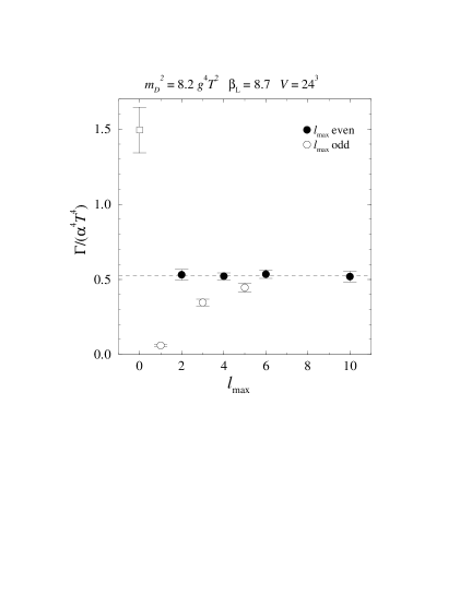
Figure 4: The dependence of $\Gamma$ on $l_{\rm max}$ on a lattice of size $24^{3}$,$\beta_{\rm L}=8.7$.

The special case $l_{\rm max}=0$ has a rate which is $\sim 3$ times larger than the $l_{\rm max}=2,4,\ldots$ rate. This is actually close to the rate measured from standard SU(2) gauge theory without any $W$ fields at the same $\beta_{\rm L}$ [18]; there the rate was $1.68\pm.03$.

This behavior is qualitatively in accord with the theoretical analysis in the abelian theory in Sect. 4. The odd $l_{\rm max}$ sector gives a substantially reduced rate because much of the infrared power is in non-propagating modes, and is therefore not available to participate in Chern-Simons number diffusion. However, for the even $l_{\rm max}$ sector we do not see the gradual decrease in the rate as predicted by the analysis in Sect. 4, the rate just snaps to the correct level immediately when the damping is turned on by going from $l_{\rm max}=0$ to $l_{\rm max}=2$. According to the requirement for minimum $l_{\rm max}$ given in Eq. (4.22), we should use $l_{\rm max}\mathop{\raise 1.29167pt\hbox{$>$\kern-7.5pt\raise-4.73611pt\hbox{$\sim$}}}0.62m_{\rm D}^{2}/g^{4}T^{2}-0.8\approx 7$ (for even $l_{\rm max}$). The naive limits given in Eq. (4.22) are obviously too strict for the non-abelian theory.

At larger $m_{\rm D}^{2}/g^{4}T^{2}$ the difference between $l_{\rm max}=2$ and higher values should be more visible. Indeed, in simulations at $m_{\rm D}^{2}/g^{4}T^{2}=20.1$, using $l_{\rm max}=2$, 4 and 6, we do observe a significant decrease in the rate as $l_{\rm max}$ increases from 2 to 4; this is shown in Table 1. Here we use a smaller lattice spacing, $\beta_{\rm L}=12.7$, and correspondingly larger volume in lattice units. In this case the required $l_{\rm max}$, according to Eq. (4.22), would be $\sim 12$. We also see an effect in the rate at $m_{\rm D}^{2}/g^{4}T^{2}=4.75$, $\beta_{\rm L}=12.7$, using $l_{\rm max}=2$ and 4.

Physical sphaleron rate:

Figure 5: The Chern-Simons number diffusion rate $\Gamma$ in physical units. Dashed line: fit to linear + second order term, Eq. (7.2); continuous line: fit to linear + a log-term, Eq. (7.4).

$\beta_{\rm L}$ $l_{\rm max}$ $V$ $(m_{\rm D}a)^{2}$ $m_{\rm D}^{2}/g^{4}T^{2}$ time$/a$ $\Gamma/\alpha^{4}T^{4}$ $\kappa^{\prime}$ 8.0 4 $24^{3}$ 0.375 2.63 10000 1.23(11) 40.5(3.6) 8.7 4 $24^{3}$ 0.766 4.68 37500 0.808(33) 47.5(1.9) 8.7 2,4,6,10 $24^{3}$ 1.59 8.20 90000 0.526(15) 54.2(1.6) 8.7 4 $24^{3}$ 3.51 16.4 25000 0.230(18) 47.5(3.7) 12.7 4 $32^{3}$ 0.291 4.84 37500 0.687(31) 46.8(1.9) 12.7 6 $32^{3}$ 0.707 8.74 20000 0.417(48) 45.8(5.2) 12.7 4,6 $32^{3}$ 1.97 20.7 82500 0.199(13) 51.7(3.5)

Table 2: The Chern-Simons diffusion rate $\Gamma$ and the parameter of the Arnold–Son–Yaffe scaling law $\kappa^{\prime}$, Eq. (7.5). If the results at different values of $l_{\rm max}$ are statistically compatible, we have taken an average over them, as indicated.

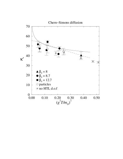
Figure 6: The Chern-Simons number diffusion rate $\Gamma$, expressed as $\kappa^{\prime}=(\Gamma/\alpha^{5}T^{4})(m_{\rm D}^{2}/(g^{2}T^{2}))$. Dashed line: fit to linear + second order term, Eq. (7.2); continuous line: fit to linear + a log-term, Eq. (7.4). For comparison, we include the results obtained with the ‘particles’ method [24] and also without any hard thermal loop degrees of freedom [18]. These points are not included in the fits.

The results for the sphaleron rate are shown in Table 2, and plotted in Figs. 5 and 6. The “old argument” [3, 4], based on dimensional analysis, says that the rate should scale as $\Gamma=\kappa\alpha^{4}T^{4}$ with $\kappa$ a constant. This behavior is clearly excluded, as already seen in [24, 18]. Rather, the rate falls linearly in $g^{4}T^{2}/m_{\rm D}^{2}$, confirming the ASY scaling picture. Indeed, we can make a fit of form

$${\frac{\Gamma}{\alpha^{4}T^{4}}}=c_{1}{\frac{g^{4}T^{2}}{m_{\rm D}^{2}}}+c_{2}\left({\frac{g^{4}T^{2}}{m_{\rm D}^{2}}}\right)^{2}$$ (7.2)

to the data, with the result $c_{1}=4.5\pm 0.2$, $c_{2}=-3.2\pm 1.1$, with $\chi^{2}=12$ for 5 degrees of freedom. Within our statistical errors, we did not observe any systematic lattice spacing dependence, and we use the results obtained with all the lattices in Table 2 in the fit. If we include the known logarithmic contribution [21],

$$\Gamma_{\log}=(0.425\pm 0.027){\frac{g^{4}T^{2}}{m_{\rm D}^{2}}}\log\left({\frac{m^{2}_{D}}{g^{4}T^{2}}}\right)\alpha^{4}T^{4}\,,$$ (7.3)

we can perform a one-parameter fit

$${\frac{\Gamma}{\alpha^{4}T^{4}}}={\frac{g^{4}T^{2}}{m_{\rm D}^{2}}}\left[0.425\log\left({\frac{m^{2}_{D}}{g^{4}T^{2}}}\right)+d\right]$$ (7.4)

with $d=3.09\pm 0.08$, with $\chi^{2}=15$ for 6 degrees of freedom. The logarithmic contribution actually makes the fit a bit worse; however, a subleading term $O(g^{4}T^{2}/m_{\rm D}^{2})$ would not change it, since its coefficient would be compatible with zero. The errors quoted above are purely statistical; we shall discuss systematic errors below.

The rate becomes approximately constant, and the difference between the two fits becomes more visible, if we plot the rate in terms of the coefficient of the ASY scaling law $\kappa^{\prime}$, defined through

$$\Gamma=\kappa^{\prime}{\frac{g^{2}T^{2}}{m_{\rm D}^{2}}}\alpha^{5}T^{4}\,.$$ (7.5)

The values of $\kappa^{\prime}$ are given in Table 2 and shown in Fig. 6. We also include here the data calculated by Moore, Hu and Müller with the particle degrees of freedom inducing the hard thermal loop effects [24], and the results obtained by Moore and Rummukainen using only SU(2) gauge fields without any additional hard thermal loop degrees of freedom [18]. In the latter case the damping arises solely through the UV gauge field modes on the lattice, and $m_{\rm D}^{2}$ can be obtained from Eq. (7.1) by setting $m_{\rm D,latt}^{2}=0$.

The consistency of the results obtained with different methods in Fig. 6 is remarkable. This gives strong credibility to the view that the damping of the sphaleron rate seen in the simulations is really caused by physical hard thermal loop effects. Perhaps surprisingly, the pure Yang-Mills results are perfectly in line (within the statistical errors) with the results obtained with the hard thermal loop effective theories, even though in the former case the spectrum of the hard modes is strongly distorted by the lattice dispersion relation [40]. Also, the consistent decrease of $\kappa^{\prime}$ with increasing $(g^{2}T/m_{D})^{2}$ in Fig. 6 strongly suggests that this subleading effect is not due to lattice effects, since the damping is due to very different mechanisms in theories with or without additional hard thermal loop degrees of freedom.

As can be seen from the $\chi^{2}$-values reported above, the quality of the fits shown in Figs. 5 and 6 is poor. This is primarily due to the ‘pull’ of the $\beta_{\rm L}=8.7$, $m_{D}^{2}=8.2\,g^{4}T^{2}$ -point, which has very small statistical errors. Exclusion of this point would make the fits acceptable; however, we do not have any a priori reason for rejecting this point, so we keep it in the analysis. We take the badness of the fits into account by expanding the errors in the quantities reported below by a factor $\sqrt{\chi^{2}/\nu}$, where $\nu$ is the number of the degrees of freedom in the fit.

In the limit $m_{D}^{2}\rightarrow\infty$ the coefficient of the ASY scaling law becomes $\kappa^{\prime}=55.9\pm 3.5$ using the polynomial function in Eq. (7.2). However, more relevant for physical applications is the Standard Model (MSM) value at $m_{\rm D}^{2}=(11/6)g^{2}T^{2}$ and $\alpha_{w}=1/30$. This corresponds to point $(g^{2}T/m_{D})^{2}=0.23$ in Fig. 6, and thus there is no need to extrapolate in $m_{D}^{2}$.

Finally, as discussed in the beginning of this section, the numerical coefficient $0.68$ in Eq. (7.1) has an estimated (quite conservative) systematic error bar $\pm 0.2$. This error has little effect on $\kappa^{\prime}$ if we extrapolate to $m_{D}^{2}\rightarrow\infty$, but at the physical MSM value it actually gives the leading contribution to the total error. When we take this into account, we obtain the physical value

$$\kappa^{\prime}(\mbox{MSM})=46.6\pm 2.0_{\rm stat}\pm 3_{\rm syst}\,,$$ (7.6)

and the MSM Chern-Simons diffusion constant becomes (with combined statistical and systematic errors)

$$\Gamma=25.4\pm 2.0\alpha^{5}T^{4}\,.$$ (7.7)

This value is in perfect agreement with the results obtained both with the particle hard thermal loop degrees of freedom [24] and with the classical Yang-Mills theory [18].

It is actually likely that the systematic error of the coefficient $(0.68\pm 0.2)$ in Eq. (7.1) is overestimated: the mutual consistency of the results obtained with and without the extra hard thermal loop degrees of freedom becomes noticeably worse when this coefficient is more than $\sim\pm 0.1$ away from the central value.

8 Conclusions

Classical Yang-Mills theory plus hard thermal loops is the IR effective theory for the SU(2) sector of the Standard Model above the electroweak phase transition, and it should be used to determine the “sphaleron rate” $\Gamma$, which sets the efficiency of baryon number violation.

We have developed a numerical implementation of the method of auxiliary fields, originally developed by Blaizot and Iancu and by Nair [25, 26, 27, 28]. The auxiliary fields are expanded in spherical harmonics and the series is truncated at a finite $l_{\rm max}$; then the theory is put on a lattice. The resulting numerical model is an efficient and systematically improvable representation of the desired effective theory.

Within errors we observe no lattice spacing dependence, and the convergence to the large $l_{\rm max}$ limit is surprisingly rapid. This means that the lattice numerical model is both accurate and efficient. Using it, we verify the Arnold-Son-Yaffe scaling behavior for $\Gamma$ [17], $\Gamma=\kappa^{\prime}(g^{2}T^{2}/m_{\rm D}^{2})\alpha^{5}T^{4}.$ If we use the Standard Model values of $m_{\rm D}^{2}=(11/6)g^{2}T^{2}$ and $\alpha_{w}=1/30$, the rate is

$$\Gamma=(25.4\pm 2.0)\alpha^{5}T^{4}~{}\simeq~{}(1.05\pm 0.08)\times 10^{-6}T^{4}\,.$$ (8.1)

The final result is in good agreement with the results previously obtained by Moore, Hu, and Müller [24]. It is also in agreement with the results obtained in pure lattice Yang-Mills theory [18] using the matching technique developed by Arnold [40] to relate $\Gamma$ in pure classical lattice Yang-Mills theory to its value in the quantum theory.

The problem of determining the sphaleron rate in Yang-Mills theory is settled, at least at the $20\%$ level.

Acknowledgments

We would like to thank Jan Ambjørn, Peter Arnold, Edmond Iancu, Arttu Rajantie, Dam Son and Larry Yaffe for several very useful discussions. This work was supported in part by the TMR network “Finite temperature phase transitions in particle physics”, EU contract no. ERBFMRXCT97-0122. The computer simulations were performed on a Cray T3E at the Center for Scientific Computing, Helsinki, Finland, and on an IBM SP2 at UNI-C computing centre, Copenhagen, Denmark.

Appendix A Spherical coefficients $v_{mi}$ and $C_{lm,l^{\prime}m^{\prime},i}$

In this appendix we give explicit expressions for the coefficients $C_{lm,l^{\prime}m^{\prime},i}$, Eq. (3.6), and $v_{mi}$, Eq. (3.5). We use the conventional normalization for the spherical harmonic functions:

$$\int{d\Omega_{v}}Y^{*}_{lm}Y_{l^{\prime}m^{\prime}}=\delta_{l,l^{\prime}}\delta_{m,m^{\prime}}\,.$$ (A.1)

The coefficients $v_{mi}$ can be given simply as

$$v_{mi} \equiv \int{d\Omega_{v}}Y^{*}_{1m}({\bf v})v_{i}$$ (A.2)

$$= \sqrt{{\frac{4\pi}{6}}}\delta_{i,1}(-\delta_{m,1}+\delta_{m,-1})+i\sqrt{{\frac{4\pi}{6}}}\delta_{i,2}(\delta_{m,1}+\delta_{m,-1})+\sqrt{{\frac{4\pi}{3}}}\delta_{i,3}\delta_{m,0}\,.$$

The matrix elements

$$C_{lm,l^{\prime}m^{\prime},i} \equiv \int{d\Omega_{v}}Y^{*}_{lm}({\bf v})v_{i}Y_{l^{\prime}m^{\prime}}({\bf v})$$ (A.3)

$$= \sum_{M}v_{Mi}\int{d\Omega_{v}}Y^{*}_{lm}({\bf v})Y_{1M}({\bf v})Y_{l^{\prime}m^{\prime}}({\bf v})$$

are conveniently expressed in terms of the spherical components

$$C_{lm,l^{\prime}m^{\prime},1} = {\frac{1}{\sqrt{2}}}(-C_{lm,l^{\prime}m^{\prime}}^{+}+C_{lm,l^{\prime}m^{\prime}}^{-})$$

$$C_{lm,l^{\prime}m^{\prime},2} = {\frac{i}{\sqrt{2}}}(C_{lm,l^{\prime}m^{\prime}}^{+}+C_{lm,l^{\prime}m^{\prime}}^{-})\,.$$

Finally, we can write

$$C_{lm,l^{\prime}m^{\prime}}^{+} = A(l^{\prime},m^{\prime})\delta_{l-1,l^{\prime}}\delta_{m-1,m^{\prime}}-A(l,-m)\delta_{l+1,l^{\prime}}\delta_{m-1,m^{\prime}}$$

$$C_{lm,l^{\prime}m^{\prime}}^{-} = A(l^{\prime},-m^{\prime})\delta_{l-1,l^{\prime}}\delta_{m+1,m^{\prime}}-A(l,m)\delta_{l+1,l^{\prime}}\delta_{m+1,m^{\prime}}$$ (A.4)

$$C_{lm,l^{\prime}m^{\prime},3} = B(l^{\prime},m^{\prime})\delta_{l-1,l^{\prime}}\delta_{m,m^{\prime}}+B(l,m)\delta_{l+1,l^{\prime}}\delta_{m,m^{\prime}}\,,$$

where the coefficients are

$$A(l,m) = \left[{\frac{(l+m+1)(l+m+2)}{2(2l+1)(2l+3)}}\right]^{1/2}\,,$$ (A.5)

$$B(l,m) = \left[{\frac{(l-m+1)(l+m+1)}{(2l+1)(2l+3)}}\right]^{1/2}\,.$$ (A.6)

Appendix B Linearized lattice propagator

In this appendix we shall study the properties of the linearized gauge field propagator with hard thermal loops on the lattice, as was done in section 4 in continuum. As emphasized in section 5, the second-order ‘leapfrog’ update for $W^{a}_{lm}$ decouples the even and odd parity sites from each other. Here parity $p=\sum_{i}x_{i}+t/\delta_{t}$. This decoupling creates extra low-energy poles, doublers , in the gauge field propagator. Here we show that these doublers are not relevant for the gauge field dynamics.

Following Sect. 4 we linearize Eqs. (5.8), (5.9) and (5.13), and study one ${\bf k}$ mode in isolation. In general, this need not be parallel to any of the major lattice axes. In Sect. 5 the spherical harmonics were written in “lattice basis” coordinates, that is, the $Y_{lm}$ components were mapped to lattice coordinate axis directions in the customary way. Naturally, there is no fundamental reason (only great convenience) to do this, and here we choose to parametrize the spherical functions as in Sect. 4, so the $Y_{lm}$ “$x_{3}$-direction” is parallel to ${\bf k}$. Then the transverse fields should oscillate only along the plane defined by $m=\pm 1$ components.

Let us make a Fourier transformation of the lattice equations of motion; after some work we obtain the equations

$$\widetilde{\omega}^{2}A_{m}-\widetilde{k}^{2}A_{m} = {\frac{m_{\rm D}^{2}}{\sqrt{3}}}D_{mm^{\prime}}\,W_{1m^{\prime}}$$ (B.1)

$$\hat{\omega}W_{lm}-\hat{k}_{i}\hat{n}_{i}C_{lm,l^{\prime}m^{\prime},3}W_{l^{\prime}m^{\prime}} = \hat{\omega}\delta_{l,1}{\frac{1}{\sqrt{3}}}D_{mM}A_{M}\,.$$ (B.2)

Here $\hat{n}={\bf k}/k$, and the lattice momentum functions are

$$\widetilde{k}_{i}={\frac{2}{a}}\sin{\frac{k_{i}a}{2}}, \widetilde{\omega}={\frac{2}{\delta_{t}a}}\sin{\frac{\omega\delta_{t}a}{2}},$$

$$\hat{k}_{i}={\frac{1}{a}}\sin k_{i}a, \hat{\omega}={\frac{1}{\delta_{t}a}}\sin\omega\delta_{t}a\,,$$ (B.3)

and the matrix $D_{mm^{\prime}}$, $m=0,\pm 1$, is defined as

$$D_{mm^{\prime}}({\bf k})=\sum_{i}\gamma_{mi}\,\cos{\frac{k_{i}a}{2}}\,\gamma^{*}_{m^{\prime}i}\hskip 11.38109pt\hskip 11.38109pt\hskip 11.38109pt\gamma_{mi}=\sqrt{{\frac{3}{4\pi}}}R_{ij}(\hat{n})v_{mj}$$ (B.4)

$R_{ij}$ is a rotation matrix which rotates $\hat{n}$ parallel to the lattice $x_{3}$-axis, and $v_{mi}$ is defined in (A.2). The matrix $\gamma$ can be understood as a transformation between the lattice coordinates and the $\hat{n}$-based spherical coordinates. Here $\gamma^{\dagger}\gamma=\gamma\gamma^{\dagger}=1$. The $\cos(k_{i}a/2)$ factor in $D_{mm^{\prime}}$ arises from the spatial symmetrization in Eqs. (5.9) and (5.13), and without this we would have $D=1$. Also, due to the timelike symmetrization $\hat{\omega}$ instead of $\widetilde{\omega}$ appears on the rhs of Eq. (B.2).

Due to the matrix $D_{mm^{\prime}}$ the equations of motion do not diagonalize to independent $m$-components, as in the continuum. However, if ${\bf k}$ is parallel to any of the lattice axes we have

$$D_{mm^{\prime}}=\delta_{m,m^{\prime}}\left(\delta_{|m|,1}+\delta_{m,0}\cos{\frac{ka}{2}}\right)\,.$$ (B.5)

In this case $D=1$ for transverse modes. Now we can solve for the transverse gauge field in Eqs. (B.1), (B.2) as in Sect. 4, and we obtain the lattice version of the inverse propagator in Eq. (4.12):

$$-\widetilde{\omega}^{2}+\widetilde{k}^{2}+{\frac{m_{\rm D}^{2}}{3}}\,\sum_{\alpha=1}^{l_{\rm max}}{\frac{\hat{\omega}}{\hat{\omega}-\hat{k}\lambda^{\alpha}}}(\xi_{1}^{\alpha})^{2}\,.$$ (B.6)

The pole structure of the propagator is not immediately evident from Eq. (B.6). Nevertheless, the propagator has new doubler poles for each physical low energy $(\omega\sim 0,k\sim 0)$ pole, as shown in Fig. 7. These are located in the corners of the momentum square $0\leq ka\leq\pi$, $0\leq\omega\delta_{t}a\leq\pi$.

    

Figure 7: Left: the positive frequency poles of the lattice gauge propagator within the Brillouin zone, as functions of $k$, for $m_{\rm D}=0.5/a$. For each of the continuum poles near origin there are doubler poles at the corners of the Brillouin zone. The thick line is the plasmon, and the dashed lines are the timelike doublers. For clarity, this figure is plotted with unrealistically large $\delta_{t}=0.75$. Right: The spectral power (residue) of the poles when $\delta_{t}=0.1$. The lines are as in the left panel. None of the doublers carry a significant fraction of the gauge field propagation.

In Fig. 7 we also show the spectral power

$$\rho(\omega,k)=\mbox{\,Im\,}\Delta(\omega+i\epsilon,{\bf k})$$ (B.7)

of the poles (residue of the propagator). At momenta close to the lattice cutoff $\pi/a$ almost all of the power is carried by the plasmon pole, which does not have doublers. Thus, at high momenta the gauge field essentially decouples from $W$ fields, except for a mass term which equals $m_{\rm D}/\sqrt{3}$ for $k$ along a lattice axis (but not everywhere, it is zero at $a{\bf k}=(\pi,\pi,\pi)$). This also occurs in the continuum. The poles other than plasmon are significant only around the physical $k,\omega\sim 0$ corner. Interestingly, even here the plasmon has a power which is a factor of $\sim 5$ larger than the other poles. However, it is these poles which are significant for the non-perturbative small-frequency physics.

One might worry about the small-$k$ temporal doublers, which correspond to modes which flip sign at each consecutive timestep: after all, these can have arbitarily long spatial wavelength. These are shown in Fig. 7 with dashed lines. However, it turns out that these poles have even much less power than the spatial doublers. Thus, the existence of the temporal poles should not affect the gauge field behavior at all. Indeed, even in non-abelian theory simulations, where the fields are fully interacting, we saw no significant energy transfer between the temporal pole sector and the ‘normal’ small frequency sector.

The propagator becomes much more complicated to study when we do not require that ${\bf k}$ is along any of the lattice axes. However, the pole structure of the propagator is qualitatively similar to any direction, and it will pick the full complement of poles at each corner of the Brillouin zone.

In order to make the left panel of Fig. 7 readable, it is plotted using $\delta_{t}=0.75$. This brings the frequency spread of the poles to the same order of magnitude than the separation between the temporal doublers and the other poles. For a more realistic $\delta_{t}\mathop{\raise 1.29167pt\hbox{$<$\kern-7.5pt\raise-4.73611pt\hbox{$\sim$}}}0.1$ the poles would lie almost along $\omega a\delta_{t}/\pi=0,1$ lines.

Appendix C O(a) matching for $\Gamma$

In this appendix we compute $O(a)$ radiative corrections which arise in the infrared dynamics of the lattice theory due to the compact nature of the gauge action and the manner in which the original equations were discretized. The goal is to find what modifications must be made to $\Gamma$ and $m_{\rm D}^{2}$ (where here $m_{\rm D}^{2}$ is really being used to represent the magnitude of the damping rate for gauge field modes with $\omega\ll k\sim g^{2}T$, which determines the relevant dynamics [17, 40]; when we write $m_{\rm D}^{2}$ we mean the value which gives the same damping rate using the continuum relation between $m_{\rm D}^{2}$ and the damping rate).

C.1 Corrections to $t$ and $m_{\rm D}^{2}$

To begin, we discuss the relation between the lattice and continuum values for $E$, $D_{j}F_{ji}$ (meaning the first term on the right hand side in Eq. (5.5)), and time $t$. Where possible we will suppress spatial and group indices, in particular we refer to $D_{j}F_{ji}$ as $DF$. We will write $E_{L}$ etc. for the lattice fields scaled to continuum units directly using Eq. (5.1), but always using $a$ as given in Eq. (5.10). The scaling between the continuum $A$ field and the lattice one, defined as $U=\exp(igaA^{a}T^{a})$, is gauge dependent, and we will always use the continuum normalization. The calculation here relies both on [34] and on Appendix A of [21] very heavily.

Define the following renormalization constants:

$$Z_{g} = \beta/\beta_{L}\simeq 1-0.61/\beta\,,$$ (C.1)

$$Z_{E} = \left[1+\frac{N}{\beta}\left(\frac{1}{3}\frac{\Sigma}{4\pi}+6\frac{\xi}{4\pi}\right)\right]\simeq 1+.314/\beta\,,$$ (C.2)

$$Z_{W} = 1-\frac{N}{2\beta}\frac{\Sigma}{4\pi}\simeq 1-0.2527/\beta\,,$$ (C.3)

where $Z_{g}$ is computed in [34] and presented above in Eq. (5.10), $Z_{E}$ is first computed in the appendix of [21] (where it has the unfortunate notation of $(1+{\rm corr})^{2}$), and $Z_{W}$ is new to this paper and discussed more in the next subsection.

To begin observe that, just from its appearance in the Hamiltonian next to $\beta_{\rm L}$, we have

$$\langle E_{L}^{2}\rangle=Z_{g}\langle E^{2}_{C}\rangle\quad\Rightarrow\quad E_{L}=Z_{g}^{1/2}E_{C}\,.$$ (C.4)

Also, from [21] Appendix A, we have

$$\frac{dA_{C}}{dt_{L}}=Z_{E}^{1/2}E_{L}=Z_{E}^{1/2}Z_{g}^{1/2}E_{C}\quad\Rightarrow\quad t_{L}=Z_{E}^{-1/2}Z_{g}^{-1/2}t_{C}\,.$$ (C.5)

We apply this correction when we extract the continuum value of $\Gamma$ from data which appear as a time series in $t_{L}$, so $\Gamma$ quoted in this paper is always scaled by $Vt_{C}$ the continuum volume and time. Next, to find the renormalization of $DF$, we can use pure gauge theory relations

$$\frac{dE_{L}}{dt_{L}}=-DF_{L}\qquad{\rm and}\qquad\frac{dE_{C}}{dt_{C}}=-DF_{C}\,,$$ (C.6)

to find that

$$DF_{L}=Z_{E}^{1/2}Z_{g}DF_{C}\,,$$ (C.7)

which we will need below.

To compute the radiative corrections in the $W$ field contribution to the gauge field damping rate we need to consider the equations of motion of the full system. If there were only infrared fields, then the first errors from our discretization (sampling neighbors to determine a derivative , $\ldots$) would enter at $O(a^{2})$, while here we will only be interested in $O(a)$ effects. Nevertheless, because of the different behavior of UV modes on the lattice than in the continuum, three new corrections arise: one in the $E$ field source in the $W$ equation of motion, Eq. (5.12); one in the $W$ field source in the Yang-Mills-Maxwell-Ampere equation, Eq. (5.5); and one in the $W$ field convective covariant derivative in Eq. (5.12). The former two occur because, whereas in the continuum these equations relate fields at the same point (see Eqs. (3.4) and (3.7)), on the lattice they involve averages over nearby points, see Fig. 8. The latter correction occurs because the derivative term necessarily involves the gauge field connection. In each case the gauge field connection enters, and the interaction receives tadpole contributions which are absent in the continuum. As a result, the effective IR equations of motion look (in a simplified notation, dropping all subscripts including $l,m$ indices and all Clebsch-Gordan coefficients, which are the same as in the text of the paper)

$$\frac{dE_{L}}{dt_{L}} = -DF_{L}-m_{\rm D}^{2}\kappa_{1}W_{L}\,,$$ (C.8)

$$\frac{dW_{L}}{dt_{L}} = \kappa_{2}E_{L}-\kappa_{3}v\cdot D_{C}W_{L}\,,$$ (C.9)

$$\kappa_{1}\kappa_{2} = Z_{W}\,,\qquad\kappa_{3}=Z^{2}_{W}\,.$$ (C.10)

Here $m_{\rm D}^{2}$ is the lattice $m_{\rm D}^{2}$ parameter converted to physical units by scaling with factors of $a$. We derive the size of the corrections $\kappa_{1,2,3}$ in the next subsection.

Figure 8: Neighbor averaging involved in the updates of $E$ due to $W$ and $W$ due to $E$.

Re-arranging Eq. (C.9) to

$$\left[\kappa_{3}^{-1}\frac{d}{dt_{L}}+v\cdot D_{C}\right]W=\kappa_{3}^{-1}\kappa_{2}E_{L}\,,$$ (C.11)

formally inverting it, and substituting the solution for $W$ into Eq. (C.8), gives

$$\frac{dE_{L}}{dt_{L}}=-DF_{L}-m_{\rm D}^{2}\left[\kappa_{3}^{-1}\frac{d}{dt_{L}}+v\cdot D_{C}\right]^{-1}\kappa_{1}\kappa_{2}\kappa_{3}^{-1}E_{L}\,.$$ (C.12)

It has been argued in [41, 42] that in the overdamped case it is permissible to drop both the $dE/dt$ term and the time derivative appearing in the inverse operator. Technically doing so commits an error of order $O(g^{4}T^{2}/m_{\rm D}^{2})$. Note however that errors of precisely this size already arise from subleading corrections to the hard classical lattice mode contribution in Eq. (7.1). Therefore, in Figure 6 there is an unknown systematic error in the slope of the fit line, which we will not be able to eliminate. However, we can still ask to make all $O(a)$ corrections which would affect the intercept. To do so we are permitted to drop the time derivatives mentioned above, giving

$$m_{\rm D}^{2}\left(Z_{W}^{-1}Z_{E}^{-1/2}Z_{g}^{-1/2}\right)\left[v\cdot D_{C}\right]^{-1}\frac{dA_{C}}{dt_{C}}=DF_{C}\,,$$ (C.13)

which gives us the $O(a)$ renormalization appropriate for the $W$ field Debye mass term, namely, the value to use as the strength of the gauge field damping term is

$$Z_{m_{D}}^{-1}m_{\rm D}^{2}\equiv Z_{W}^{-1}Z_{E}^{-1/2}Z_{g}^{-1/2}\>m_{\rm D}^{2}\,.$$ (C.14)

C.2 Evaluating $\kappa_{1,2,3}$

We see from Fig. 8 that the product $\kappa_{1}\kappa_{2}$ arises from the difference between $W^{a}(x)$ and $(1/4)[{\cal P}^{ab}_{i}W^{b}(x+ia)+2W^{a}(x)+{\cal P}^{ab}_{-i}W^{b}(x-ia)]$. We compute this difference for a very slowly varying $W$ field in Coulomb gauge. (In this gauge the effects of the $A_{0}$ field on the dynamics do not differ between the lattice and continuum, see [21].)

The parallel transport ${\cal P}^{ab}_{i}W^{b}(x+ia)$ is

$$T^{c}(U_{i}(x)W_{+}U^{\dagger}_{i}(x))^{c} = \left(1+igaT^{a}A_{i}^{a}(x)-\frac{g^{2}a^{2}}{2}T^{a}T^{b}A^{a}_{i}(x)A^{b}_{i}(x)+\ldots\right)$$ (C.15)

$$\qquad\times T^{c}W^{c}\times\bigg{(}{\rm same},\;i\leftrightarrow-i\bigg{)}\,,$$

and on expanding (and writing $(1/4)(W(x+ia)+2W(x)+W(x-ia))$ as $W$) eventually gives

$$\frac{{\cal P}^{ab}_{i}W^{b}(x+ia)+2W^{a}(x)+{\cal P}^{ab}_{-i}W^{b}(x-ia)}{4}$$ (C.16)

$$= W^{a}T^{a}+\frac{ga}{4}W^{b}\left(A^{c}_{i}(x)-A^{c}_{i}(x-ia)\right)f_{abc}T^{a}$$

$$+\frac{g^{2}a^{2}}{8}W^{a}\left(A^{b}_{i}(x)A^{c}_{i}(x)+A^{b}_{i}(x-ia)A^{c}_{i}(x-ia)\right)[T^{c},[T^{a},T^{b}]]+O(a^{3})\,.$$

In momentum space the first term here is $-f^{abc}(ga^{2}/4)\int_{l}\tilde{l}_{i}W^{b}(l-k)A^{c}_{i}(-l)$. It cannot lead to a contribution proportional to $W(k)$ because $\langle f^{abc}W^{a}(k)W^{b}(l-k)A^{c}(-l)\rangle=0$. Therefore the first term does not rescale the interaction, so it does not contribute to $\kappa_{1}\kappa_{2}$. However, the last term does lead to renormalization of $W^{a}T^{a}$, of magnitude

$$f_{adb}f_{bde}T^{e}\frac{g^{2}aT}{4}\int\frac{d^{3}(ak)}{(2\pi)^{3}}\frac{1}{a^{2}\tilde{k}^{2}}\left(1-\frac{\tilde{k}_{1}^{2}}{\tilde{k}^{2}}\right)\cos^{2}(ak_{1}/2)\,,$$ (C.17)

where $\tilde{k}\equiv(2/a)\sin(ak/2)$ and the integral runs over the Brillioun zone, $ak_{i}\in[-\pi,\pi]$. Using identities from [34], the value of the integral is $(1/2)\Sigma/(4\pi)$. Therefore the final rescaling we find is

$$\kappa_{1}\kappa_{2}\equiv Z_{W}=1-\frac{N}{2\beta}\frac{\Sigma}{4\pi}\,.$$ (C.18)

The calculation of $\kappa_{3}$ proceeds similarly. Here we need to compute $({\cal P}^{ab}_{i}W^{b}(x+ia)-{\cal P}^{ab}_{-i}W^{b}(x-ia))/2$. The linear in $A$ term now contains $A_{i}(x)+A_{i}(x-ia)$, and just gives the $A$ field part of the continuum $D^{ab}_{i}=\delta^{ab}\partial_{i}-gf_{abc}A^{c}_{i}$. The quadratic in $A$ terms perform the renormalization of $\partial_{i}$ and give exactly twice the corresponding contribution to $\kappa_{1}\kappa_{2}$, because in that case only half of the expression arose from $W$ fields which are parallel transported. Hence we find $\kappa_{3}=Z_{W}^{2}$.

References

- [1] G. t’Hooft, Phys. Rev. Lett. 37,8 (1976).
- [2] V.A. Kuzmin, V.A. Rubakov and M.E. Shaposhnikov, Phys. Lett. B155, 36 (1985).
- [3] P. Arnold and L. McLerran, Phys. Rev. D 36, 581 (1987).
- [4] S. Khlebnikov and M. Shaposhnikov, Nucl. Phys. B308, 885 (1988).
- [5] E. Mottola and S. Raby, Phys. Rev. D 42, 4202 (1990).
- [6] V. Rubakov and M. Shaposhnikov, Phys. Usp. 39, 461 (1996) [Usp. Fiz. Nauk 166, 493 (1996)] [hep-ph/9603208].
- [7] P. Arnold and L. McLerran, Phys. Rev. D 37, 1020 (1988).
- [8] D. Grigoriev and V. Rubakov, Nucl. Phys. B 299, 248 (1988).
- [9] J. Ambjørn, T. Askgaard, H. Porter, and M. Shaposhnikov, Nucl. Phys. B 353, 346 (1991).
- [10] J. Ambjørn and A. Krasnitz, Phys. Lett. B 362, 97 (1995) [hep-ph/9508202].
- [11] G.D. Moore, Nucl. Phys. B 480, 657 (1996) [hep-ph/9603384]; ibid. B 480, 689 (1996) [hep-lat/9605001].
- [12] W. Tang and J. Smit, Nucl. Phys. B482, 265 (1996) [hep-lat/9605016].
- [13] J. Ambjørn and A. Krasnitz, Nucl. Phys. B506, 387 (1997) [hep-ph/9705380].
- [14] G.D. Moore and N. Turok, Phys. Rev. D56, 6533 (1997) [hep-ph/9703266].
- [15] G.D. Moore, Phys. Rev. D59, 014503 (1999) [hep-ph/9805264].
- [16] D. Bödeker, L. McLerran and A. Smilga, Phys. Rev. D52, 4675 (1995) [hep-th/9504123].
- [17] P. Arnold, D. Son and L.G. Yaffe, Phys. Rev. D55, 6264 (1997) [hep-ph/9609481].
- [18] G.D. Moore and K. Rummukainen, MCGILL-99/21, NORDITA-99/33HE [hep-ph/9906259].
- [19] D. Bödeker, Phys. Lett. B 426, 351 (1998) [hep-ph/9801430].
- [20] P. Arnold, D. Son, and L.G. Yaffe, Phys. Rev. D 59, 105020 (1999) [hep-ph/9810216].
- [21] G.D. Moore, MCGILL/98-28 [hep-ph/9810313].
- [22] J. Taylor and S. Wong, Nucl. Phys. B 346, 115 (1990); J. Frenkel and J. Taylor, Nucl. Phys. B 374, 156 (1992); E. Braaten and R. Pisarski, Phys. Rev. D 45, 1827 (1992).
- [23] C.R. Hu and B. Müller, Phys. Lett. B409, 377 (1997) [hep-ph/9611292].
- [24] G.D. Moore, C. Hu and B. Müller, Phys. Rev. D58, 045001 (1998) [hep-ph/9710436].
- [25] J.P. Blaizot and E. Iancu, Phys. Rev. Lett. 70, 3376 (1993) [hep-ph/9301236].
- [26] V.P. Nair, Phys. Rev. D48, 3432 (1993) [hep-ph/9307326].
- [27] J. Blaizot and E. Iancu, Nucl. Phys. B421, 565 (1994) [hep-ph/9401211].
- [28] V.P. Nair, Phys. Rev. D50, 4201 (1994) [hep-th/9403146].
- [29] G.D. Moore and N. Turok, Phys. Rev. D55, 6538 (1997) [hep-ph/9608350].
- [30] D. Bödeker, Nucl. Phys. B486, 500 (1997) [hep-th/9609170].
- [31] A. Rajantie and M. Hindmarsh, SUSX-TH-99-002 [hep-ph/9904270].
- [32] E. Braaten and R. Pisarski, Nucl. Phys. B337, 569 (1990); J. Frenkel and J. Taylor, Nucl. Phys. B334, 199 (1990);
- [33] J. Kogut and L. Susskind, Phys. Rev. D 11, 395 (1975).
- [34] G.D. Moore, Nucl. Phys. B493, 439 (1997) [hep-lat/9610013]; Nucl. Phys. B523, 569 (1998) [hep-lat/9709053].
- [35] K. Kajantie, K. Rummukainen and M. Shaposhnikov, Nucl. Phys. B407, 356 (1993) [hep-ph/9305345].
- [36] K. Kajantie, M. Laine, K. Rummukainen and M. Shaposhnikov, Nucl. Phys. B458, 90 (1996) [hep-ph/9508379].
- [37] A. Krasnitz, Nucl. Phys. B455, 320 (1995) [hep-lat/9507025].
- [38] M. Lüscher, Comm. Math. Phys. 85, 39 (1982).
- [39] P. Woit, Phys. Rev. Lett. 51, 638 (1983); Nucl. Phys. B 262, 284 (1985).
- [40] P. Arnold, Phys. Rev. D55, 7781 (1997) [hep-ph/9701393].
- [41] P. Huet and D.T. Son, Phys. Lett. B393, 94 (1997) [hep-ph/9610259].
- [42] D.T. Son, UW/PT-97-19 [hep-ph/9707351].