Symmetry breaking via fermion 4-point functions

Abstract

We construct the effective action and gap equations for nonperturbative fermion 4-point functions. Our results apply to situations in which fermion masses can be ignored, which is the case for theories of strong flavor interactions involving standard quarks and leptons above the electroweak scale. The structure of the gap equations is different from what a naive generalization of the 2-point case would suggest, and we find for example that gauge exchanges are insufficient to generate nonperturbative 4-point functions when the number of colors is large.

Contents

toc

I Introduction

In theories without elementary scalar fields, electroweak symmetry breaking is accomplished through the dynamical generation of fermion masses of order a TeV. This chiral symmetry breaking must somehow be fed down to the lighter quark and lepton masses to produce their mass spectrum. The original “extended technicolor” idea was to accomplish this via broken gauge interactions, with symmetry breaking scales ranging up to $\sim 1000$ TeV. There are two main problems with this idea. One is that it immediately raises the question of what breaks these new interactions. What plays the role of the order parameter for this breakdown? If it is another mass-type order parameter then it must involve new fermions with exotic quantum numbers, since conventional quarks and leptons are not allowed to have mass above the electroweak breaking scale. The other problem is that the complicated structure of the quark and lepton mass spectrum is directly reflected in the structure of the new gauge interactions. This led to models having an input structure (in the form of the symmetry and representation content) no less complicated than the output structure (the quark and lepton mass spectrum), and basically the whole extended technicolor idea gradually sank under its own weight.

Our motivation for the current work comes from the well know fact that there is a much richer set of possible order parameters which may be utilized by a strongly interacting theory, beyond the simple mass-type order parameter. Therefore the order parameters that signal the breakdown of flavor symmetries could actually be constructed out of the known quarks and leptons, due to their participation in strong flavor dynamics at high scales. The only constraint is that these order parameters respect electroweak symmetry, which in turn ensures that quarks and leptons do not develop masses on these scales and thus remain in the theory below the flavor scale. Among such $SU(2)_{L}\times U(1)$ invariant order parameters are ones involving four fermions. They will result in effective 4-fermion interactions in the low energy theory, and thus the same order parameters responsible for breaking flavor symmetries can be responsible for feeding down the TeV masses to lighter quark and leptons. The difference from extended technicolor models is that we now have a larger class of possible operators, and the variety in size and structure of these operators must be a reflection of strong dynamics, rather than a reflection of some input structure.

We mention in passing that there are 2-fermion order parameters involving standard quarks and leptons, of the chirality preserving type, which could serve as flavor breaking order parameters. If right-handed neutrinos are appended to the standard model set of fermions, then a Majorana-mass-type order parameter could also be considered. In this work we shall restrict ourselves to the study of the more diverse set of 4-fermion order parameters, which we shall refer to as (nonperturbative) 4-point functions.

We are entertaining the possibility that strong interactions dynamically break various flavor symmetries, but preserve $SU(2)_{L}\times U(1)$. For this to happen the gauge interactions may have to be chiral, so that the gauge interactions themselves resist the formation of masses. For example a competition between different gauge interactions could end up reducing the attraction in the mass channels. In nonchiral theories as well, it could simply be that the critical coupling required for the formation of a more symmetric 4-point function is less than that for any 2-point function. In any case we stress that any strongly interacting theory of flavor above the electroweak scale must preserve $SU(2)_{L}\times U(1)$. With the neglect of fermion masses the chirality structure of the various 4-point functions will be the focus of our attention, and we often keep the flavor and gauge structures implicit. The chirality structure is constrained by $SU(2)_{L}\times U(1)$ symmetry and in particular 4-point functions having an odd number of each chirality, such as $\langle\overline{\psi}\partial\!\!\!/\psi\psi\overline{\psi}\rangle$ are excluded.

To illustrate this discussion consider a strong $SU(N_{c})$ gauge interaction for an even number $N_{f}>2$ of massless fermions in the fundamental representation of the gauge group. The flavor symmetry is $SU(N_{f})_{L}\times SU(N_{f})_{R}\times U(1)_{V}$. The chirality preserving 4-point functions can be made invariant under this chiral symmetry, while the chirality changing 4-point functions cannot be invariant. The formation of the latter can still be consistent with a chiral isospin (or ‘electroweak’) symmetry and a vector ‘family’ symmetry,

$$SU(2)_{L}\times SU(2)_{R}\times SU(N_{f}/2)_{V}\times U(1)_{V}.$$ (1)

The corresponding chirality changing 4-point functions have the structure

$$\left\langle\left(\overline{\psi}_{R}^{Aa}\psi_{L}^{Ab}\right)\epsilon_{ac}\epsilon_{bd}\left(\overline{\psi}_{R}^{Bc}\psi_{L}^{Bd}\right)\right\rangle,$$ (2)

where the upper case superscripts denote family, the lower case superscripts denote isospin and $\epsilon_{ac}$ is a $2\times 2$ anti-symmetric matrix.

An investigation into the nonperturbative generation of 4-point functions requires knowledge of the effective action and gap equations of the 4-point functions. We use the procedures in [1] to derive these tools in a general context. Before we present the detailed derivations, we provide an overview which summarizes the derivations. We will also explore the solutions to the gap equations in the framework of the model of the previous paragraph, in the large $N_{c}$ limit.

II Overview of the derivations

More than three decades ago De Dominicis and Martin published a set of papers [1] in which they provide procedures for the derivation of gap equations and effective actions for various $n$-point Green functions. Although their analysis was presented in the framework of non-relativistic statistical physics the procedures can be readily applied to quantum field theory. We follow their procedure for 4-point functions to derive the effective action and gap equations in the context of gauge theories with massless fermions.

Below we review their procedure in its adapted form. We are only interested in the part of their analysis dealing with 4-point functions. There are two parts to this procedure, which can be regarded as two independent ways to derive the required gap equations. One part provides a direct derivation of these equations. The other part is a derivation of the effective action, from which one can then reproduce the same gap equations by imposing a stationarity condition of the form

$${\delta\Gamma\over\delta C}=0,$$ (3)

where $C$ denotes a 4-point function. Although the direct method is perhaps a quicker method to obtain the expressions for the gap equations, it is the other method which actually makes a statement about the vacuum of the theory by showing that these gap equations extremize the effective action.

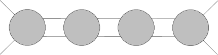
FIG. 1.: A bubble chain

The direct method is presented in detail in Sec. V. The goal is to derive the gap equations for the five 4-point functions as presented in (V D). Schematically they are all of the form

$$C=T_{s}(C)+T_{d}(C)+T_{d}^{T}(C)+K(C,g)$$ (4)

where $C$ is a connected, amputated 4-point function. The $T$’s are sums of bubble chains, shown in Fig. 1, formed by connecting $C$’s through pairs of fermion lines. There are three different bubble chains because there are three ways to pair off the four external lines of a 4-point function. The subscript $s$ ($d$) indicates that the fermion lines in each pair have the same (opposite) direction. The superscript $T$ indicates that the two incoming or two outgoing lines are interchanged, with ‘incoming’ and ‘outgoing’ referring to the arrows on the external fermion lines. Only the $K$-term depends on the gauge coupling explicitly, and it contains all the 4-particle irreducible (4PI) diagrams that one can form from these $C$’s together with the other propagators and vertices of the gauge theory. The diagrams are also 2-particle irreducible (2PI) since the fermion line represents the full fermion propagator. We are assuming that the fermion propagator itself does not break any symmetries and in particular is massless.

The main task in the direct derivation of the gap equations is to find the expressions for the $T$’s in terms of the $C$’s; here we sketch the procedure. We require the following definition: when a 4-point diagram cannot be separated into two parts where each part has a pair of the original external lines, by cutting two internal fermion lines, the 4-point diagram is said to be simple with respect to this particular pairing of external lines. The sum of all 4-point diagrams that are simple with respect to one specific pairing of external lines is denoted by $U$. One can define $T$ as the sum of all 4-point diagrams that are simple with respect to all but the aforementioned pairing of external lines. (A 4-point function can only be nonsimple with respect to one pairing, which follows from the absence of fermion 3-point functions.) Then $C=U+T$ for this pairing of external lines. Since there are three ways of pairing off the four external lines one can define three $U$’s and three $T$’s.

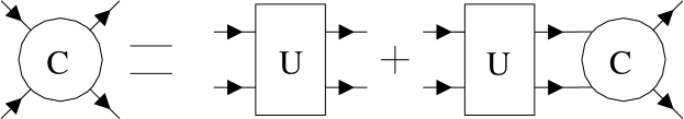
FIG. 2.: Master equation

Next, a master equation relates $C$ to one of the three $U$’s, for a particular pairing of external lines. The equation, shown diagrammatically in Fig. 2, can be written as

$$C=U+UC.$$ (5)

The 2-line connection of the $U$ to the $C$ is presented as a product of two 4-point functions in (5). This notation will be used throughout the rest of this paper, and it will be discussed further in Sec. V A. From (5) it directly follows that

$$U=C[1+C]^{-1},$$ (6)

and thus the $T$-term in the gap equation for a particular pairing is given by

$$T=C-U=C^{2}[1+C]^{-1}.$$ (7)

The actual derivations of the various $T$’s which appear in the five gap equations are more involved. The different chiralities lead to sets of more complicated master equations which are to be solved simultaneously to obtain the expressions for the $U$’s and the $T$’s. The expressions of these $T$’s are provided in (67), (V B 3), (V B 3) and (V B 3).

As discussed in Sec. V C the $K$-term is simple with respect to all pairings. It can be generated from the sum of all 4PI vacuum diagrams through the following functional derivation

$$K[C]=\left[{\delta V_{4PI}[C]\over\delta C}\right]_{amp}.$$ (8)

Here $V_{4PI}[C]$ denotes the sum of all 4PI vacuum diagrams in which the 4-point function, $C$, is treated as a 4-point vertex. The subscript $amp$ indicates that the diagrams are amputated. The $K$-term together with the expressions for the $T$’s completes the derivation of the gap equations in (V D).

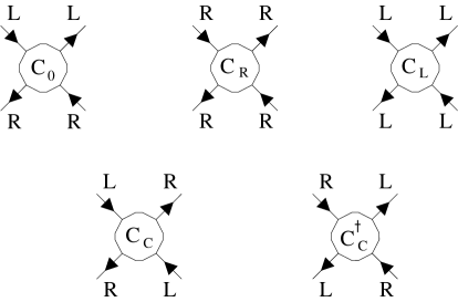
FIG. 3.: The five connected, amputated 4-point functions

Next we present an overview of the derivation of the effective action from which one can derive the same gap equations. The resulting expression for the effective action as a functional of the various $C$’s is

$$\Gamma = {\rm Tr}\left\{\ln\left(1-\frac{1}{4}R_{s}C^{{\dagger}}L_{s}C\right)_{s}+\ln\left(1+\frac{1}{2}C_{R}\right)_{s}+\ln\left(1+\frac{1}{2}C_{L}\right)_{s}+\ln(1+C_{0})_{s}\right.$$ (12)

$$+\frac{1}{2}\ln\left(1-RC_{0}LC_{0}\right)_{d}+\frac{1}{2}\ln\left(1+C_{R}\right)_{d}+\frac{1}{2}\ln\left(1+C_{L}\right)_{d}+\ln\left(1+C_{0}\right)_{d}$$

$$+\frac{1}{2}\ln\left(1-ZC^{{\dagger}}ZC\right)_{d}-C_{R}-C_{L}-2C_{0}$$

$$\left.+\frac{1}{2}CC^{{\dagger}}+C_{0}^{2}+\frac{1}{4}C_{R}^{2}+\frac{1}{4}C_{L}^{2}\right\}+V_{4PI}[C,C^{{\dagger}},C_{0},C_{R},C_{L}].$$

The five different $C$’s which appear in this expression are defined as follows (see Fig. 3). When all four of the external lines of a 4-point function have the same chirality, say left-handed (right-handed), we denote the 4-point function by $C_{L}$ ($C_{R}$). These two 4-point functions are chirality preserving. The other chirality preserving 4-point function, which we denote by $C_{0}$, has one incoming and one outgoing line of each chirality. The remaining two 4-point functions are chirality changing; their incoming and outgoing lines have the opposite chirality. When the chirality of their incoming lines are left-handed (right-handed) we denote them by $C_{C}$ ($C_{C}^{{\dagger}}$). The other symbols which appear in this expression are defined as follows

$$R_{s} = \left[1+\frac{1}{2}C_{R}\right]_{s}^{-1}$$ (14)

$$L_{s} = \left[1+\frac{1}{2}C_{L}\right]_{s}^{-1}$$ (15)

$$R = \left[1+C_{R}\right]_{d}^{-1}$$ (16)

$$L = \left[1+C_{L}\right]_{d}^{-1}$$ (17)

$$Z = \left[1+C_{0}\right]_{d}^{-1},$$ (18)

where the subscript $s$ and $d$ have the same meaning as in (4). The formulation of these objects and how they are applied in the derivation of the effective action are discussed in Sec. V A.

The effective action is the Legendre transform of the sum of all connected vacuum diagrams in the presence of the 4-fermion sources. The $J$-dependence is replaced by a $C$-dependence, and thus the aim is to find an expression for the effective action in terms of the 4-point functions ($C$’s) with only implicit dependence on the sources ($J$’s). The problem is to avoid overcounting. This problem is solved in [1] by adding and subtracting various sets of diagrams in such a way that the overcounting is eliminated and the original sum of vacuum diagrams is retained. This is done with the aid of the following topological equation, which is proved in [1].

$$1=N_{skel}+N_{vert}-N_{art}+\sum_{pair~{}cycles}[1-N_{p}+N_{pp}]$$ (19)

Each term in this equation denotes the number of a specific element or feature (such as skeletons or pair cycles) which is present in a vacuum diagram. These terms and the way they are applied to vacuum diagrams are explained in Section VI A,VI B. The topological relation relates the numbers of times a diagram is overcounted when considering the various manifestations of the various features. It is useful because, by distinguishing a specific feature of the vacuum diagrams, one can generate the associated term from the $C$’s. In other words, the topological equation will allows us to express the sum of all connected vacuum diagrams in terms of various sets of vacuum diagrams which can be explicitly constructed from the 4-point functions.

By performing functional derivatives with respect to the various $C$’s on the effective action in (12), one can reproduce the exact expressions for the gap equations. This is shown in Sec. VII. The expressions for the effective action and the gap equations represent the main result of our analysis, which extends to 4-point functions the CJT analysis [2] of 2-point functions. The structure of our equations are different from what a naive extension of the CJT analysis would suggest, and this is made evident in the following application.

III Gap equations in the large $N_{c}$ limit

The above discussion summarizes the program carried out in the rest of the paper. In this section we will make a first attempt to use the resulting formalism to extract information about the 4-point functions. We will treat the model described in the introduction, a $SU(N_{c})$ gauge theory with $N_{f}$ fermions, each having $N_{c}$ colors. Although such a theory is not chiral, we can still look for any intrinsic tendency of the theory to produce nonperturbative 4-point functions. We consider a large $N_{c}$ expansion to simplify the structure of the gap equations. We then need to know the leading $N_{c}$-dependences of the $C$’s. Note that the gap equations contain sequences of 4-point functions of the form $[1+C]^{-1}$. In these sequences adjacent $C$’s are interconnected with two fermion lines, which can form color loops, and each color loop gives a factor of $N_{c}$. In the large $N_{c}$ limit these sequences would only be convergent and nontrivial if the $C$’s themselves are $O(1/N_{c})$. This is true for all types of $C$’s.

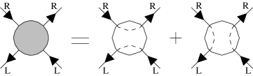
FIG. 4.: Color structures of $C_{0}$.

The next step is to separate each of the different $C$’s into color structures. If the color indices on the external lines of $C$ are $a,b,\overline{c}$ and $\overline{d}$, then one can connect these indices internally in the following two ways: $\delta^{a\overline{c}}\delta^{b\overline{d}}$ or $\delta^{a\overline{d}}\delta^{b\overline{c}}$. $C_{0}$ does not have any symmetry with respect to interchanges of external lines and so in this case the two color structures represent two different objects,

$$C_{0}=C_{0V}+C_{0S}.$$ (20)

These color structures are shown in Fig. 4, where the dashed lines indicate how the color indices are connected internally. The connected indices have the same chirality for $C_{0V}$ and the opposite chirality for $C_{0S}$. The two color structures for the other $C$’s are just transposed versions of the same object. By ‘transposed’ we mean that the two lines with the outgoing fermion arrows are interchanged, or equivalently the two incoming lines are interchanged. We denote a particular color structure of these $C$’s with a hat, and to reconstruct the original $C$ we write

$$C=\hat{C}+(\hat{C})^{T}.$$ (21)

The $1/N_{c}$ expansion is obtained by substituting (20) and (21) into the various expressions, paying attention to the color loops formed by the various color structure orientations of the $C$’s.

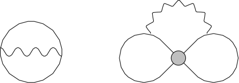
FIG. 5.: The two 4PI vacuum diagrams with one-gauge-boson exchanges

The great simplification that occurs is due to the fact that the diagrams in $V_{4PI}$ at leading order in $1/N_{c}$ contain no more than one 4-point function each. The two vacuum diagrams that are leading order in $1/N_{c}$, as well as being leading order in $\alpha$, are shown in Fig. 5. Because the fermions are massless the single 4-point function that appears in the second diagram in Fig. 5 is chirality preserving. All the other diagrams in $V_{4PI}$ involving a 4-point function at leading order in $1/N_{c}$ also look similar to this diagram. The single gauge boson is just replaced by the set of 4PI planar graphs. We denote the sum of all these vacuum diagrams by Fig. 6a and the 4-point diagram that is obtained after removing the 4-point function by Fig. 6b.

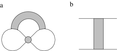
FIG. 6.: The 4PI gauge interaction vacuum and 4-point diagrams at leading order in $1/N_{c}$.

The expression for the effective action at leading order in $1/N_{c}$ splits into two parts. These two parts decouple from each other because they do not share the same $C$’s. One part is

$$\Gamma_{1}={\rm Tr}\left\{\frac{1}{2}\ln\left(1-\hat{C}_{C}\hat{Z}\hat{C}_{C}^{{\dagger}}\hat{Z}\right)_{d}+\ln\left(1+C_{0S}\right)_{d}-C_{0S}\right\}+V_{4PI,1}$$ (22)

where $\hat{Z}=[1+C_{0S}]_{d}^{-1}$ and $V_{4PI,1}$ contains the diagram in Fig. 6a with $C_{0S}$ as the 4-point function. The other part is

$$\Gamma_{2} = {\rm Tr}\left\{\frac{1}{2}\ln\left(1-C_{0V}\hat{L}C_{0V}\hat{R}\right)_{d}+\frac{1}{2}\ln\left(1+\hat{C}_{R}\right)_{d}+\frac{1}{2}\ln\left(1+\hat{C}_{L}\right)_{d}-\frac{1}{2}\hat{C}_{R}-\frac{1}{2}\hat{C}_{L}\right\}$$ (24)

$$+V_{4PI,2}$$

where $\hat{R}=[1+\hat{C}_{R}]_{d}^{-1}$, $\hat{L}=[1+\hat{C}_{L}]_{d}^{-1}$ and $V_{4PI,2}$ contains the diagram in Fig. 6a with $C_{L}$ or $C_{R}$ as the 4-point function. The gap equations associated with (22) are

$$\hat{C}_{C}=T_{d},~{}~{}~{}\hat{C}_{C}^{{\dagger}}=T^{{\dagger}}_{d}~{}~{}~{}{\rm and}~{}~{}~{}C_{0S}=T^{0}_{d}+K_{0}$$ (25)

and those for (24) are

$$\hat{C}_{R}=T^{R}_{d}+K_{R},~{}~{}~{}\hat{C}_{L}=T^{L}_{d}+K_{L}~{}~{}~{}{\rm and}~{}~{}~{}C_{0V}=T^{\prime}_{d}.$$ (26)

The various $T$’s are provided in (67), (V B 3), (V B 3) and (V B 3), and the various $K$’s appear in (V D). The gap equations for $\hat{C}_{C}$ and $\hat{C}_{C}^{{\dagger}}$ do not have $K$-terms, because we have seen that in the large $N_{c}$ limit the 4PI vacuum diagrams are independent of $\hat{C}_{C}$ and $\hat{C}_{C}^{{\dagger}}$. The expression for $C_{0V}$ in (26) also does not have a $K$-term, because the color structure of the would-be $K$-term does not match. It shows up in the $C_{0S}$-expression in (25) instead.

Consider the first set of gap equations in (25), where we look first at $\hat{C}_{C}$ (or equivalently $\hat{C}_{C}^{{\dagger}}$). From the expression for $T_{d}$, given in (125), we have:

$$\hat{C}_{C}=\hat{C}_{C}-\hat{Z}\hat{C}_{C}\hat{Z}\left[1-\hat{C}_{C}^{{\dagger}}\hat{Z}\hat{C}_{C}\hat{Z}\right]_{d}^{-1}$$ (27)

where $\hat{Z}=[1+C_{0S}]_{d}^{-1}$. It is clear that the only solution for this expression is $\hat{C}_{C}=0$, irrespective of what the value of $C_{0S}$ is. This happens because the equation does not have a $K$-term.

Using the expression for $T^{0}_{d}$, (127), the gap equation for $C_{0S}$ becomes:

$$C_{0S}=C_{0S}+\hat{Z}\left[1-\hat{C}_{C}^{{\dagger}}\hat{Z}\hat{C}_{C}\hat{Z}\right]_{d}^{-1}-1+X_{0}.$$ (28)

Here $X_{0}$, which is a contribution from the $K$-term, denotes the 4PI planar graphs in Fig. 6b, with the chiralities of the external fermion lines the same as $C_{0}$. For $\hat{C}_{C}=\hat{C}_{C}^{{\dagger}}=0$, (28) gives

$$C_{0S}=X_{0}\left[1-X_{0}\right]_{d}^{-1},$$ (29)

which implies that $C_{0S}$ is generated perturbatively by the sum of ‘ladder’ diagrams, with each rung the set of 4PI planar graphs.

A 4-point function of the $C_{0S}$ form may have a nontrivial flavor structure which would prevent it from being generated perturbatively, i.e. its gap equation would not have a $K$-term:

$$C_{0S}=\hat{C}_{C}^{{\dagger}}\hat{Z}\hat{C}_{C}.$$ (30)

In this case it is only possible to generate a nonperturbative $C_{0S}$ indirectly through $\hat{C}_{C}$ and $\hat{C}_{C}^{{\dagger}}$, if the latter were nonzero.

Consider next the other set of gap equations in (26). Using the expression for $T^{\prime}_{d}$, (120), the gap equation for $C_{0V}$ becomes

$$C_{0V}=C_{0V}-\hat{R}C_{0V}\hat{L}\left[1-C_{0V}\hat{R}C_{0V}\hat{L}\right]_{d}^{-1}$$ (31)

where $\hat{R}=[1+\hat{C}_{R}]_{d}^{-1}$ and $\hat{L}=[1+\hat{C}_{L}]_{d}^{-1}$. This is very similar to (27), and again the only solution is $C_{0V}=0$. As for $\hat{C}_{R}$ (or $\hat{C}_{L}$), by using the expression for $T^{R}_{d}$ (122) we obtain

$$\hat{C}_{R}=\hat{C}_{R}+\hat{R}\left[1-C_{0V}\hat{L}C_{0V}\hat{R}\right]_{d}^{-1}-1+X_{R}.$$ (32)

Here $X_{R}$ denotes the 4PI planar graphs in Fig. 6b where the chiralities of the external fermion lines are those of a $C_{R}$. This gives

$$\hat{C}_{R}=X_{R}\left[1-X_{R}\right]_{d}^{-1}$$ (33)

since $C_{0V}=0$. Hence, just like $C_{0S}$, $\hat{C}_{R}$ is generated perturbatively by a ‘ladder’ sum of 4PI planar graphs.

The absence of nonperturbative solutions of gap equations for 4-point functions seems counterintuitive in the light of the situation which is so well known for 2-point functions[4]. The naive generalization of the linearized ladder gap equation for the fermion self-energy to 4-point functions would be of the form

$$C_{C}=EC_{C}$$ (34)

where $E$ is the one gauge exchange kernel. Equations of this type were considered in [5, 6]. The reason we do not obtain such an equation can be traced to the absence in $V_{4PI}$ of the diagram consisting of two 4-point functions and one-gauge-boson exchange, shown in Fig. 7a. Its absence is independent of the $1/N_{c}$ expansion and is due simply to the fact that this diagram is not 4PI. This diagram is implicitly included in the $T$-terms in (4) (since the chirality preserving 4-point functions implicitly have one-gauge-boson exchange contributions), and we have seen that the $T$-terms by themselves cannot generate nonperturbative solutions. Note that the diagram involving a triple gauge vertex, shown in Fig. 7b, is included in $V_{4PI}$, but this contribution is subleading in $1/N_{c}$.

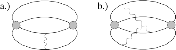
FIG. 7.: Vacuum diagrams with two 4-point functions.

In light of these results it is of interest to consider the possible effects of instantons, which lie outside of our current approach. Due to the chirality changing nature of instanton effects, they may lead to the dynamical generation of the chirality changing 4-point functions, $\hat{C}_{C}$ and $\hat{C}_{C}^{{\dagger}}$. We note that the lines of a ’t Hooft-vertex operator[3] can be closed off with chirality changing 4-point functions, and that the diagram containing chirality changing 4-point functions only (no chirality preserving 4-point functions) would be leading in $1/N_{c}$. Thus it may be the case that at leading order in $1/N_{c}$, $\hat{C}_{C}$ and $\hat{C}_{C}^{{\dagger}}$ are generated dynamically by instanton effects. $C_{0S}$ would then be affected as in (30).

We are finding then a qualitative difference between the 2-point function case and the 4-point function case, in the large $N_{c}$ limit. None of the 4-point functions can be generated dynamically by gauge exchanges, and only the chirality changing 4-point functions, $C_{C}$ and $C_{C}^{{\dagger}}$, could in principle be dynamically generated via instanton effects. We remind the reader that these particular 4-point functions are relevant to the symmetry breaking pattern in (1), which is of special interest for models of flavor physics which preserve electroweak symmetries.

We now present the detailed derivation of the gap equations and the effective action. First we present the general formulation and notation in Sec. IV. The direct derivation of the gap equations is presented in Sec. V while Sec. VI contains the derivation of the effective action. In Sec. VII we show that the gap equations minimize the effective action.

IV Green functions and 4-point functions

In order to extend the CJT analysis [2] to treat 4-point functions, one can introduce a nonlocal 4-fermion source term in addition to the nonlocal 2-fermion source term. The generating functional is then given by,

$$W^{\prime}[j,J]=-i\ln\left[\int\exp\left(iS+iS_{j}+iS_{J}\right){\cal D}\right],$$ (35)

where $S$ is the action of the gauge theory and ${\cal D}$ is the functional measure over all the fields in the theory. Schematically

$$S_{j} = \int\overline{\psi}(x_{1})j(x_{1},x_{2})\psi(x_{2})\ d^{4}x_{1}d^{4}x_{2}$$ (36)

$$S_{J} = \int\overline{\psi}(x_{1})\psi(x_{2})J(x_{1}...x_{4})\overline{\psi}(x_{3})\psi(x_{4})\ d^{4}x_{1}...d^{4}x_{4}.$$ (37)

Here $j$ denotes the nonlocal 2-fermion source and $J$ denotes the nonlocal 4-fermion source. The generating functional, $W^{\prime}[j,J]$, is the sum of all connected vacuum diagrams which one can construct by using the Feynman rules of a gauge theory, together with the sources as 2-fermion and 4-fermion vertices.

We perform two Legendre transforms on this generating functional to arrive at the effective action. The first Legendre transformation,

$$\Gamma_{CJT}[S,J]=W^{\prime}[j,J]-\int j\cdot S,$$ (38)

replaces the functional dependences $j$ by a functional dependences on the full fermion propagator $S$, which is expressed as

$$S=\frac{\delta W^{\prime}}{\delta j}.$$ (39)

$\Gamma_{CJT}[S,J]$ is the CJT effective action [2] in the presence of four-fermion sources. The stationarity condition

$$\frac{\delta\Gamma_{CJT}[S,J]}{\delta S}=0,$$ (40)

provides a way to determine the full propagator $S$ up to a dependence on the 4-fermion source.

At this point it would be opportune to discuss the chiral properties of the Green functions. There are five nonlocal 4-fermion source terms which are for this purpose included in the action, and so the 4-fermion source term in (35) becomes

$$S_{J} = \int\left(\frac{1}{4}\overline{\psi}_{R}(x_{1})\psi_{L}(x_{2})J_{C}(x_{1}...x_{4})\overline{\psi}_{R}(x_{3})\psi_{L}(x_{4})\right.$$ (45)

$$+\frac{1}{4}\overline{\psi}_{L}(x_{1})\psi_{R}(x_{2})J_{C}^{{\dagger}}(x_{1}...x_{4})\overline{\psi}_{L}(x_{3})\psi_{R}(x_{4})$$

$$+\overline{\psi}_{R}(x_{1})\psi_{L}(x_{2})J_{0}(x_{1}...x_{4})\overline{\psi}_{L}(x_{3})\psi_{R}(x_{4})$$

$$+\frac{1}{4}\overline{\psi}_{R}(x_{1})\psi_{R}(x_{2})J_{R}(x_{1}...x_{4})\overline{\psi}_{R}(x_{3})\psi_{R}(x_{4})$$

$$\left.+\frac{1}{4}\overline{\psi}_{L}(x_{1})\psi_{L}(x_{2})J_{L}(x_{1}...x_{4})\overline{\psi}_{L}(x_{3})\psi_{L}(x_{4})\right)\ d^{4}x_{1}...d^{4}x_{4}.$$

The sources with the subscript $C$ are associated with chirality changing Green functions, while the other three sources are chirality preserving. Four of the source terms have the same chiralities on both $\psi$-fields, as well as on both $\overline{\psi}$-fields. Thus the symmetry associated with the identical incoming pair and the identical outgoing pair introduces the symmetry factor of $\frac{1}{4}$. The color and flavor indices of the fermion fields are contracted on the sources.

$\Gamma_{CJT}[S,J]$ can be expressed as the sum of one-loop terms, $-{\rm Tr}\{\ln(S^{-1})\}+{\rm Tr}\{(S^{-1}-\partial\!\!\!/)S)\}$, which are independent of the 4-fermion sources, and $W[S,J]$, the set of connected 2PI vacuum diagrams with fermion lines representing the full propagator. From now on we will treat the $W[S,J]$ as our generating functional.

The second Legendre transform gives the effective action of interest,

$$\Gamma^{\prime}[S,G]=W[S,J]-\int\left(\frac{1}{4}J_{C}G_{C}^{{\dagger}}+\frac{1}{4}J_{C}^{{\dagger}}G_{C}+J_{0}G_{0}+\frac{1}{4}J_{R}G_{R}+\frac{1}{4}J_{L}G_{L}\right)\ d^{4}x_{1}...d^{4}x_{4}.$$ (46)

The Green functions are given by the functional derivatives of the generating functional with respect to the appropriate sources,

$${\delta W\over\delta J_{C}^{{\dagger}}}=G_{C},~{}~{}~{}{\delta W\over\delta J_{C}}=G_{C}^{{\dagger}},~{}~{}~{}{\delta W\over\delta J_{0}}=G_{0},~{}~{}~{}{\delta W\over\delta J_{R}}=G_{R}~{}~{}~{}{\rm and}~{}~{}~{}{\delta W\over\delta J_{L}}=G_{L}.$$ (47)

Both the sources and the Green functions have color and flavor indices. The effective action obeys the following stationarity conditions

$${\delta\Gamma^{\prime}[S,G]\over\delta G_{C}^{{\dagger}}}=0,~{}~{}~{}{\delta\Gamma^{\prime}[S,G]\over\delta G_{C}}=0,~{}~{}~{}{\delta\Gamma^{\prime}[S,G]\over\delta G_{0}}=0,~{}~{}~{}{\delta\Gamma^{\prime}[S,G]\over\delta G_{R}}=0~{}~{}~{}{\rm and}~{}~{}~{}{\delta\Gamma^{\prime}[S,G]\over\delta G_{L}}=0.$$ (48)

Now we see that in spite of the fact that the addition of a nonlocal 4-fermion source term would change the full propagator, it is consistent to fix $S$ and vary only the Green function $G$. Throughout our discussions we assume a general massless propagator,

$$S(p)=i{Z(p)\over p\!\!\!/}.$$ (49)

It is also more convenient to write the effective action as a functional of the connected and amputated parts of the Green functions. These objects are denoted by the symbol $C$ and we shall refer to them as 4-point functions to distinguish them from the Green functions,

$$C(x_{1}...x_{4})=\left[\langle T\overline{\psi}_{1}\psi_{2}\overline{\psi}_{3}\psi_{4}\rangle-\langle T\overline{\psi}_{1}\psi_{2}\rangle\langle T\overline{\psi}_{3}\psi_{4}\rangle-\langle T\overline{\psi}_{1}\psi_{4}\rangle\langle T\overline{\psi}_{3}\psi_{2}\rangle\right]_{amp},$$ (50)

where the Green function is

$$G=\langle T\overline{\psi}_{1}\psi_{2}\overline{\psi}_{3}\psi_{4}\rangle.$$ (51)

The 4-point functions, $C$’s, are classified in the same way as the Green functions (recall Fig. 3 and the discussion below (12)). Therefore in place of $\Gamma^{\prime}[S,G]$ we consider $\Gamma[C]$, in terms of which the stationarity conditions become

$${\delta\Gamma[C]\over\delta C_{C}^{{\dagger}}}=0,~{}~{}~{}{\delta\Gamma[C]\over\delta C_{C}}=0,~{}~{}~{}{\delta\Gamma[C]\over\delta C_{0}}=0,~{}~{}~{}{\delta\Gamma[C]\over\delta C_{R}}=0~{}~{}~{}{\rm and}~{}~{}~{}{\delta\Gamma[C]\over\delta C_{L}}=0.$$ (52)

These conditions are equivalent to (48) because the full propagators are held constant. The stationarity of the effective action with respect to the 4-point functions ($C$’s) contains the nonperturbative information we are trying to extract.

The derivation of the effective action involves finding a diagrammatic representation in which the five terms that are removed through the Legendre transformation are the only ones with explicit sources. All other source terms should end up inside subdiagrams which are replaced by explicit $C$’s, so that we have a formula for $\Gamma$ which contains no reference to $J$.

V Direct derivation of the gap equations

The gap equations we seek will be expressed in terms of 2PI diagrams constructed out of the 4-point functions (treated as a 4-point vertex), 2-point functions (our full fermion propagator) and the vertices and propagators associated with a gauge theory. We do not need the 4-fermion sources for the derivation in this section, they will appear again in Sec. VI. Some diagrams will contain gauge interactions explicitly while others will not, and it is by balancing these two sets of diagrams that one can find a nontrivial solution for the 4-point functions under investigation. The infinite set of diagrams with explicit gauge interaction cannot, of course, be given in closed form, while a set of the diagrams consisting only of 4-point functions and fermion propagators can be. The latter set are the bubble chains (see Fig. 1) which consist of sequences of 4-point functions.

A Preliminaries

1 Types of fermion pairs

We first describe our notation. All the 4-point functions which are considered here (that is, all the $C$’s, $U$’s and $T$’s, which are defined below) are amputated. Therefore, when two of these 4-point functions are connected by two fermion lines, two fermion propagators are to be inserted between the two 4-point functions. We shall leave this step implicit in our notation, and so $C_{C}C_{C}^{{\dagger}}$ really means $C_{C}SSC_{C}^{{\dagger}}$. Since $S$ is chirality preserving the product of two 4-point functions is only possible if the directions and chiralities of the fermion lines that are to be connected are compatible. This may depend on the type of 4-point function (a $C_{C}$ can never by directly connected to another $C_{C}$) or on the type of fermion pairs.

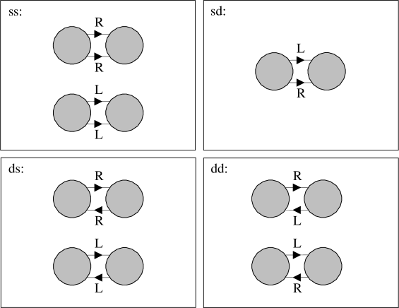
FIG. 8.: Four types of fermion pairs that can connect 4-point functions.

We define four types of fermion pairs depending on the directions and chiralities of the fermion lines which connect two adjacent 4-point functions. Each type of fermion pair is denoted by two letters, the first of which is associated with the directions and the second with the chiralities of the fermion lines. We use s and d to denote ‘same’ and ‘different’ respectively. $ss$, $sd$, $ds$, or $dd$ will appear as subscripts on objects or brackets to indicate that the objects or the enclosed expressions have a specific type of fermion pairs, as illustrated in Fig. 8. Often only one of these letters will appear in the subscript; in such a case the letter denotes the directions and not the chiralities, with the latter being clear from the context.

2 Simple 4-point functions

A 4-point diagram is said to be simple with respect to a particular pairing of external lines when it cannot be separated into two parts, each having one pair of the original external lines, by cutting two internal fermion lines in the 4-point diagram. We denote the sum of all 4-point diagrams that are simple with respect to one specific pairing of external lines by $U$ and refer to it as a simple 4-point function. We use $T$ to denote the sum of all 4-point diagrams that are simple with respect to all but a specific pairing of external lines. Then the 4-point function, $C$, is the sum of a $U$ and a $T$ associated with a specific pairing:

$$C=U+T.$$ (53)

(For a while we shall not distinguish the different chiralities.) There are three ways of pairing off four external lines. One can therefore define three $U$’s and three $T$’s. Any particular 4-point diagram is either nonsimple with respect to only one of these pairings or it is simple with respect to all three pairings. It thus follows that $C$ can be written as the sum of three $T$’s (one for each possible pairing) and $K$, which is the sum of all diagrams that are simple with respect to all pairings:

$$C=T+T+T+K.$$ (54)

The $T$’s are the various bubble chains that can be resummed in closed form.

Once we distinguish between left-handed and right-handed fermions we have the five $C$’s defined in Sec. II below (12) (see also Fig. 3). The chirality preserving 4-point functions are $C_{0}$, $C_{R}$ and $C_{L}$ and the chirality changing 4-point functions are $C_{C}$ and $C_{C}^{{\dagger}}$.

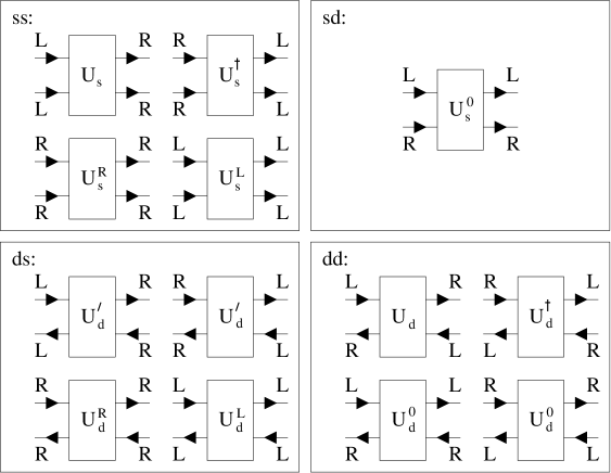
FIG. 9.: The definition of the simple 4-point functions ($U$’s) in terms of the pairings and chiralities of the external lines. The four groups indicate the four different types of fermion pairs.

Each simple 4-point function is defined with respect to one type of fermion pair. The four categories of $U$’s are shown in Fig. 9. In summary: for the ss-fermion pairs we have $U_{s}$, $U_{s}^{{\dagger}}$, $U_{s}^{R}$ and $U_{s}^{L}$; there is only one for the sd-fermion pairs, namely $U_{s}^{0}$; those for the ds-fermion pairs are $U_{d}^{\prime}$, $U_{d}^{R}$ and $U_{d}^{L}$; and the dd-fermion pairs are $U_{d}$, $U_{d}^{{\dagger}}$ and $U_{d}^{0}$. Note that $U_{d}^{\prime}$ and $U_{d}^{0}$ appear twice each in Fig. 9. There is a $T$ for every $U$. They are related by (53) for each specific pairing of the external lines of the particular $C$.

It will be useful to define a set of bubble sums that are formed as the sum of sequences of the same $U$ or $C$. There are only some of these $U$’s and $C$’s that can form such sequences. The bubble sums involving $C$’s are given in (II) in Sec. II. Those involving $U$’s are

$$R_{s}^{U} = \left[1-\frac{1}{2}U_{s}^{R}\right]_{ss}^{-1}$$ (56)

$$L_{s}^{U} = \left[1-\frac{1}{2}U_{s}^{L}\right]_{ss}^{-1}$$ (57)

$$R^{U} = \left[1-U_{d}^{R}\right]_{ds}^{-1}$$ (58)

$$L^{U} = \left[1-U_{d}^{L}\right]_{ds}^{-1}$$ (59)

$$B = \left[1-U_{d}^{0}\right]_{dd}^{-1}.$$ (60)

Although one can also define such an object for the sd-fermion pairs, it does not appear often enough to merit its definition. The factor of $\frac{1}{2}$ that appears in (14), (15), (56) and (57) removes the overcounting due to the identical fermion lines in the cases with ss-fermion pairs. When we encounter this symmetry again it will be referred to as the ss-symmetry.

There are other types of transformations which play an important role in some of the derivations of the subsequent sections, especially in Sec. VII. For this purpose we define the following transformations, which are denoted by superscripts. Assume that $G$ is an object with four external lines paired off as $(1,2)$ and $(3,4)$. Then one can define the following three transformations:

$$\left[G(1,2;3,4)\right]^{T} = G(1,3;2,4)$$ (62)

$$\left[G(1,2;3,4)\right]^{F} = G(2,1;4,3)$$ (63)

$$\left[G(1,2;3,4)\right]^{R} = G(3,4;1,2).$$ (64)

The last one is referred to as a back-to-front transformation.

B The T-terms

1 The master equations

Each master equation expresses a 4-point function ($C$) in terms of some simple 4-point function ($U$) and itself, and leads to an expression for the $U$ in terms of the $C$. The $T$-term then follows as the difference between the $C$ and this $U$. We have four types of fermion pairs, three of which have four master equations each. The remaining fermion pair type has only one master equation, and we start our discussion with this equation.

$C_{0}$ is the only $C$ that can have the sd-fermion pair type. The associated simple 4-point function is $U_{s}^{0}$ and the master equation is (see Fig. 2):

$$C_{0}=U_{s}^{0}+U_{s}^{0}C_{0}.$$ (65)

From (65) it then directly follows that

$$U_{s}^{0}=C_{0}[1+C_{0}]_{sd}^{-1}.$$ (66)

The $T$-term in the gap equation for $C_{0}$ is now given by

$$T_{s}^{0}=C_{0}-U_{s}^{0}=C_{0}^{2}[1+C_{0}]_{sd}^{-1}.$$ (67)

For the other three types of fermion pairs we first present all the master equations. The master equations for the ss-fermion pairs are:

$$C_{C} = U_{s}+\frac{1}{2}U_{s}^{L}C_{C}+\frac{1}{2}U_{s}C_{R}$$ (69)

$$C_{C}^{{\dagger}} = U_{s}^{{\dagger}}+\frac{1}{2}U_{s}^{R}C_{C}^{{\dagger}}+\frac{1}{2}U_{s}^{{\dagger}}C_{L}$$ (70)

$$C_{R} = U_{s}^{R}+\frac{1}{2}U_{s}^{R}C_{R}+\frac{1}{2}U_{s}^{{\dagger}}C_{C}$$ (71)

$$C_{L} = U_{s}^{L}+\frac{1}{2}U_{s}^{L}C_{L}+\frac{1}{2}U_{s}C_{C}^{{\dagger}}.$$ (72)

The factor, $\frac{1}{2}$, is due to the ss-symmetry mentioned at the end of Sec. V A. Next we have the master equations for the ds-fermion pairs:

$$C_{0} = U_{d}^{\prime}+U_{d}^{R}C_{0}+U_{d}^{\prime}C_{L}$$ (74)

$$C_{0} = U_{d}^{\prime}+U_{d}^{L}C_{0}+U_{d}^{\prime}C_{R}$$ (75)

$$C_{R} = U_{d}^{R}+U_{d}^{R}C_{R}+U_{d}^{\prime}C_{0}$$ (76)

$$C_{L} = U_{d}^{L}+U_{d}^{L}C_{L}+U_{d}^{\prime}C_{0}.$$ (77)

The first two equation, (74) and (75), and the last terms in the last two equation, (76) and (77), may seem ambiguous. Note, however, that corresponding external lines of different terms in an equation must have the same directions and chiralities. As a result one can see that (74) and (75) are related by a back-to-front transformation, as defined in (64) and that the fermion lines which connect $C_{0}$ and $U_{d}^{\prime}$ are left-handed in (76) and right-handed in (77).

The final set of master equations are for the dd-fermion pairs:

$$C_{C} = U_{d}+U_{d}C_{0}+U_{s}^{0}C_{C}$$ (79)

$$C_{C}^{{\dagger}} = U_{d}^{{\dagger}}+U_{d}^{{\dagger}}C_{0}+U_{d}^{0}C_{C}^{{\dagger}}$$ (80)

$$C_{0} = U_{d}^{0}+U_{d}^{0}C_{0}+U_{d}^{{\dagger}}C_{C}$$ (81)

$$C_{0} = U_{d}^{0}+U_{d}^{0}C_{0}+U_{d}C_{C}^{{\dagger}}.$$ (82)

The last term in each of (81) and (82) define the chirality assignments on the external lines and thence the definition of the other terms follow unambiguously.

2 Simple 4-point functions

The master equations are manipulated to give the $U$’s expressed in terms of only the $C$’s. The expressions of the $U$’s are required for the pair cycle terms of the effective action which are derived in Sec. VI B. From the twelve expressions in (V B 1), (V B 1) and (V B 1) one can write down simpler expressions using the definitions in (II) and (¶ ‣ V A 2). First we consider the ss-fermion pairs in detail. With the use of the definitions in (14), (15), (56) and (57) the expressions in (69) and (70) become

$$C_{C}R_{s}=L_{s}^{U}U_{s}$$ (84)

and

$$C_{C}^{{\dagger}}L_{s}=R_{s}^{U}U_{s}^{{\dagger}}.$$ (85)

Using the same definitions one can express the next two equations, (71) and (72) as

$$1=R_{s}^{U}R_{s}+\frac{1}{4}R_{s}^{U}U_{s}^{{\dagger}}C_{C}R_{s}=R_{s}^{U}R_{s}+\frac{1}{4}C_{C}^{{\dagger}}L_{s}C_{C}R_{s}$$ (86)

and

$$1=L_{s}^{U}L_{s}+\frac{1}{4}L_{s}^{U}U_{s}C_{C}^{{\dagger}}L_{s}=L_{s}^{U}L_{s}+\frac{1}{4}C_{C}R_{s}C_{C}^{{\dagger}}L_{s},$$ (87)

where we have used the identities in (84) and (85). From (86) and (87) one can now write down the expressions for $U_{s}^{R}$ and $U_{s}^{L}$:

$$U_{s}^{R}=2-2R_{s}\left[1-\frac{1}{4}C_{C}^{{\dagger}}L_{s}C_{C}R_{s}\right]_{s}^{-1}$$ (89)

and

$$U_{s}^{L}=2-2L_{s}\left[1-\frac{1}{4}C_{C}R_{s}C_{C}^{{\dagger}}L_{s}\right]_{s}^{-1}.$$ (90)

One can eliminate $R_{s}^{U}$ between (85) and (86) to find an expression for $U_{s}^{{\dagger}}$,

$$U_{s}^{{\dagger}}=R_{s}C_{C}^{{\dagger}}L_{s}\left[1-\frac{1}{4}C_{C}R_{s}C_{C}^{{\dagger}}L_{s}\right]_{s}^{-1}$$ (91)

and similarly one can eliminate $L_{s}^{U}$ between (84) and (87) to find an expression for $U_{s}$,

$$U_{s}=L_{s}C_{C}R_{s}\left[1-\frac{1}{4}C_{C}^{{\dagger}}L_{s}C_{C}R_{s}\right]_{s}^{-1}.$$ (92)

In the derivation of these equations we have used the identity

$$A\left[1-BA\right]^{-1}=\left[1-AB\right]^{-1}A.$$ (93)

The ds-fermion pairs and dd-fermion pairs follow the same steps. The equivalent expressions for the ds-fermion pairs are:

$$C_{0}L = R^{U}U_{d}^{\prime}$$ (95)

$$C_{0}R = L^{U}U_{d}^{\prime}$$ (96)

$$1 = R^{U}R+R^{U}U_{d}^{\prime}C_{0}R=R^{U}R+C_{0}LC_{0}R$$ (97)

$$1 = L^{U}L+L^{U}U_{d}^{\prime}C_{0}L=L^{U}L+C_{0}RC_{0}L.$$ (98)

From these we derive the expressions for the following $U$’s:

$$U_{d}^{R} = 1-R\left[1-C_{0}LC_{0}R\right]_{d}^{-1}$$ (100)

$$U_{d}^{L} = 1-L\left[1-C_{0}RC_{0}L\right]_{d}^{-1}$$ (101)

$$U_{d}^{\prime} = RC_{0}L\left[1-C_{0}RC_{0}L\right]_{d}^{-1}$$ (102)

$$U_{d}^{\prime} = LC_{0}R\left[1-C_{0}LC_{0}R\right]_{d}^{-1}.$$ (103)

The last two equations, (102) and (103), are related through a back-to-front transformation. The expressions for the dd-fermion pairs are:

$$C_{C}Z = BU_{d}$$ (105)

$$C_{C}^{{\dagger}}Z = BU_{d}^{{\dagger}}$$ (106)

$$1 = BZ+BU_{d}^{{\dagger}}C_{C}Z=BZ+C_{C}^{{\dagger}}ZC_{C}Z$$ (107)

$$1 = BZ+BU_{d}C_{C}^{{\dagger}}Z=BZ+C_{C}ZC_{C}^{{\dagger}}Z,$$ (108)

and from them follow the expressions for the remaining $U$’s:

$$U_{d}^{0} = 1-Z\left[1-C_{C}ZC_{C}^{{\dagger}}Z\right]_{d}^{-1}$$ (110)

$$U_{d}^{0} = 1-Z\left[1-C_{C}^{{\dagger}}ZC_{C}Z\right]_{d}^{-1}$$ (111)

$$U_{d} = ZC_{C}Z\left[1-C_{C}^{{\dagger}}ZC_{C}Z\right]_{d}^{-1}$$ (112)

$$U_{d}^{{\dagger}} = ZC_{C}^{{\dagger}}Z\left[1-C_{C}ZC_{C}^{{\dagger}}Z\right]_{d}^{-1}.$$ (113)

Here the first two equations, (110) and (111), are related through a back-to-front transformation.

3 T-term expressions

The final step in the derivation of the $T$-terms in the gap equation is to use equations of the form $T=C-U$ to find their expressions. The expressions for the $U$’s are those provided in (66), (87), (V B 2) and (V B 2). This step is quite straight forward so we merely quote all the relevant expressions.

ss-fermion pairs:

$$T_{s} = C_{C}-U_{s}=\frac{1}{2}U_{s}^{L}C_{C}+\frac{1}{2}U_{s}C_{R}=C_{C}-L_{s}C_{C}R_{s}\left[1-\frac{1}{4}C_{C}^{{\dagger}}L_{s}C_{C}R_{s}\right]_{s}^{-1}$$ (115)

$$T_{s}^{{\dagger}} = C_{C}^{{\dagger}}-U_{s}^{{\dagger}}=\frac{1}{2}U_{s}^{R}C_{C}^{{\dagger}}+\frac{1}{2}U_{s}^{{\dagger}}C_{L}=C_{C}^{{\dagger}}-R_{s}C_{C}^{{\dagger}}L_{s}\left[1-\frac{1}{4}C_{C}R_{s}C_{C}^{{\dagger}}L_{s}\right]_{s}^{-1}$$ (116)

$$T_{s}^{R} = C_{R}-U_{s}^{R}=\frac{1}{2}U_{s}^{R}C_{R}+\frac{1}{2}U_{s}^{{\dagger}}C_{C}=C_{R}+2R_{s}\left[1-\frac{1}{4}C_{C}^{{\dagger}}L_{s}C_{C}R_{s}\right]_{s}^{-1}-2$$ (117)

$$T_{s}^{L} = C_{L}-U_{s}^{L}=\frac{1}{2}U_{s}^{L}C_{L}+\frac{1}{2}U_{s}C_{C}^{{\dagger}}=C_{L}+2L_{s}\left[1-\frac{1}{4}C_{C}R_{s}C_{C}^{{\dagger}}L_{s}\right]_{s}^{-1}-2$$ (118)

ds-fermion pairs:

$$T_{d}^{\prime} = C_{0}-U_{d}^{\prime}=U_{d}^{R}C_{0}+U_{d}^{\prime}C_{L}=C_{0}-RC_{0}L\left[1-C_{0}RC_{0}L\right]_{d}^{-1}$$ (120)

$$T_{d}^{\prime} = C_{0}-U_{d}^{\prime}=U_{d}^{L}C_{0}+U_{d}^{\prime}C_{R}=C_{0}-LC_{0}R\left[1-C_{0}LC_{0}R\right]_{d}^{-1}$$ (121)

$$T_{d}^{R} = C_{R}-U_{d}^{R}=U_{d}^{R}C_{R}+U_{d}^{\prime}C_{0}=C_{R}+R\left[1-C_{0}LC_{0}R\right]_{d}^{-1}-1$$ (122)

$$T_{d}^{L} = C_{L}-U_{d}^{L}=U_{d}^{L}C_{L}+U_{d}^{\prime}C_{0}=C_{L}+L\left[1-C_{0}RC_{0}L\right]_{d}^{-1}-1$$ (123)

dd-fermion pairs:

$$T_{d} = C_{C}-U_{d}=U_{d}C_{0}+U_{s}^{0}C_{C}=C_{C}-ZC_{C}Z\left[1-C_{C}^{{\dagger}}ZC_{C}Z\right]_{d}^{-1}$$ (125)

$$T_{d}^{{\dagger}} = C_{C}^{{\dagger}}-U_{d}^{{\dagger}}=U_{d}^{{\dagger}}C_{0}+U_{d}^{0}C_{C}^{{\dagger}}=C_{C}^{{\dagger}}-ZC_{C}^{{\dagger}}Z\left[1-C_{C}ZC_{C}^{{\dagger}}Z\right]_{d}^{-1}$$ (126)

$$T_{d}^{0} = C_{0}-U_{d}^{0}=U_{d}^{0}C_{0}+U_{d}^{{\dagger}}C_{C}=C_{0}+Z\left[1-C_{C}^{{\dagger}}ZC_{C}Z\right]_{d}^{-1}-1$$ (127)

$$T_{d}^{0} = C_{0}-U_{d}^{0}=U_{d}^{0}C_{0}+U_{d}C_{C}^{{\dagger}}=C_{0}+Z\left[1-C_{C}ZC_{C}^{{\dagger}}Z\right]_{d}^{-1}-1$$ (128)

A back-to-front transformation relates (120) and (121), as well as (127) and (128).

C 4-particle irreducible diagrams

The $K$-term contains all 4-point diagrams that are simple with respect to all pairings of external lines. We want to express this sum of diagrams in terms of the $C$’s. That means that we have to recast the set of diagrams in the $K$-term such that all the 4-point subdiagrams inside these diagrams are contained inside $C$’s. This process is neatly performed by constructing all the 4-particle irreducible (4PI) diagrams, using the $C$’s as 4-fermion vertices, together with the full fermion propagator and the other vertices and propagators of a gauge theory. First we give the formal definition of a 4PI diagram. Then we clarify this definition.

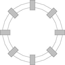
FIG. 10.: A pair cycle with eight fermion pairs – i.e. an 8-cycle. The shaded rectangles denote simple subdiagrams.

4PI 4-point diagrams are defined by first defining 4PI vacuum diagrams. The 4PI 4-point diagrams are then obtained from these vacuum diagrams by removing one 4-fermion vertex ($C$). The definition of a 4PI vacuum diagram will make use of the concept of a pair cycle, where pair refers to a pair of fermion lines. A pair cycle is a loop of pairs of fermion lines that connect simple subdiagrams to form a vacuum diagram. An example is shown in Fig. 10. A pair cycle with $\mu$ pairs is referred to as a $\mu$-cycle. Cutting the lines of all $\mu$ pairs in a $\mu$-cycle would separate the vacuum diagram into $\mu$ disconnected simple 4-point functions. If one and only one of the simple subdiagrams in a $\mu$-cycle is just a 4-fermion vertex ($C$), the $\mu$-cycle is said to be a trivial $\mu$-cycle.

The formal definition of a 4PI vacuum diagram is then that all the pair cycles in a 4PI vacuum diagram are either nontrivial 1-cycles or trivial 2-cycles.

Let’s clarify this definition by considering the requirements for 4PI diagrams and giving motivations for these requirements. For 2PI vacuum diagrams one simply requires that it should not be possible to separate the diagram into two parts by cutting two different fermion lines in the diagram. Generalizing this rule to four fermion lines for 4PI diagrams is not enough, because then no 4PI diagram would contain a $C$. So one must add that if by cutting four different fermion lines in a diagram, it separates into two parts with one and only one part being a 4-fermion vertex ($C$), then the diagram is 4PI. Thus we allow trivial two-cycles.

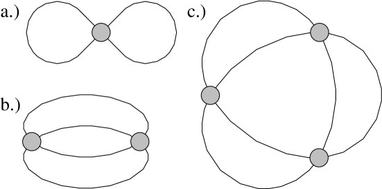
FIG. 11.: Three vacuum diagrams that are not 4PI. The shaded circles denote 4-point vertices ($J$’s or $C$’s).

A vacuum diagram that consists of two $C$’s with their lines connected to each other, as shown in Fig. 11b, produces the 4-fermion vertex ($C$) upon removal of one of the $C$’s. The latter 4-point diagram is by definition not part of $K$, and thus nontrivial 2-cycles are excluded in the definition of 4PI vacuum diagrams.

We could have tried to define 4PI vacuum diagrams as all vacuum diagrams that cannot be separated into two disconnected parts by cutting four fermion lines, unless one and only one of the parts is just the 4-fermion vertex, $C$. However, this definition still includes the diagram consisting of three $C$’s, shown in Fig. 11c. This diagram must be excluded because it becomes a diagram in $T$ when one removes one of the $C$’s. Thus we see why the definition of 4PI vacuum diagrams must exclude all diagrams with 3-cycles and higher.

Now we can obtain all the 4PI 4-point diagrams from the 4PI vacuum diagrams by cutting out (or opening up) one 4-fermion vertex ($C$). As an example: if a 4PI vacuum diagram contains five 4-fermion vertices then one can form five 4PI 4-point diagrams from it. If two or more of these 4PI 4-point diagrams are identical the original vacuum diagram would have a symmetry factor which cancels the overcounting.

The amputated 4PI 4-point diagrams that are constructed from the $C$’s, the full fermion propagators and the other vertices and propagators of a gauge theory, are exactly those which are contained in the $K$-term. To see this, remember that the $C$’s represent the sets of all connected amputated 4-point diagrams with the appropriate chiralities on their external lines. By replacing the $C$’s inside the 4PI diagrams with these sets of 4-point diagrams, one generates all the 4-point diagrams which are simple with respect all pairings of external lines. Amputating these simple diagrams, one obtains the set of diagrams which form $K$.

$$K[C]=\left[{\delta V_{4PI}[C]\over\delta C}\right]_{amp}$$ (129)

$V_{4PI}[C]$ denotes the sum of all 4PI vacuum diagrams containing the 4-point functions ($C$) as 4-point vertices.

D The gap equations

The expansions for the five 4-point functions in terms of the $T$’s and $K$’s are:

$$C_{C} = T_{s}+T_{d}+(T_{d})^{T}+K_{C}$$ (131)

$$C_{C}^{{\dagger}} = T^{{\dagger}}_{s}+T^{{\dagger}}_{d}+(T^{{\dagger}}_{d})^{T}+K_{C}^{{\dagger}}$$ (132)

$$C_{0} = T^{0}_{s}+T^{0}_{d}+T^{\prime}_{d}+K_{0}$$ (133)

$$C_{R} = T^{R}_{s}+T^{R}_{d}+(T^{R}_{d})^{T}+K_{R}$$ (134)

$$C_{L} = T^{L}_{s}+T^{L}_{d}+(T^{L}_{d})^{T}+K_{L}.$$ (135)

Note that there are always two of the $T$’s with subscript $d$ and only one $T$ with subscript $s$. The superscript $T$ indicates that the two incoming or two outgoing lines are interchanged. There is only one of the equations where the two $T$’s with subscript $d$ are different – the equation for $C_{0}$. The distinction is that for $T^{0}_{d}$ the chiralities in a pair are opposite and for $T^{\prime}_{d}$ the chiralities in a pair are the same. (This is the same as for $U^{0}_{d}$ and $U^{\prime}_{d}$, shown in Fig. 9.)

When distinguishing the chiralities, one has five different 4-point functions on which $V_{4PI}$ depends. The $K$-term in each specific expression in (V D) is generated by taking the functional derivative of $V_{4PI}$ with respect to the appropriate 4-point function. (For $K$ ($K^{{\dagger}}$) one must take the functional derivative with respect to $C^{{\dagger}}$ ($C$).) The expressions for all the $T$’s are provided in (67), (V B 3), (V B 3) and (V B 3). These expressions, together with the definitions in (II), now complete the gap equations in (V D).

Next we derive the effective action, which leads to the same gap equations.

VI Derivation of the effective action

We must find an expression for the effective action in terms of the 4-point functions ($C$’s) as outlined in Sec. IV. It requires the use of the 4-fermion sources, $J$’s, which are shown in (45). We consider all the connected 2PI vacuum diagrams that can be generated with these sources treated as 4-fermion vertices, our full fermion propagator, and other vertices and propagators of a gauge theory. The sum of all these vacuum diagrams is the generating functional, $W(S,J)$. The effective action is obtained by performing a Legendre transform, which replaces the source dependence by a dependence on the 4-point functions ($C$’s). The challenge is therefore to express $W$ in terms of $C$’s, which only implicitly depend on the $J$’s.

In the sections below we show how this is achieved with the aid of a topological equation, which allows us to avoid overcounting diagrams. The various terms in the topological equation are explained below.

A Topological equation

The topological equation,

$$1=N_{skel}-N_{art}+N_{vert}+\sum_{pair~{}cycles}[1-N_{p}+N_{pp}],$$ (136)

which is proved in [1], is an index theorem for different numbers of elements which are present in vacuum diagrams. The quantities on the right-hand side, which we shall define shortly, indicate the number of particular elements which are present in any specific vacuum diagram. Thus for any vacuum diagram, if one determines the number of each type of element which it contains, then adds or subtracts these numbers in the way indicated in (136), the result is equal to unity. (See also the discussion in Sec. II.)

The idea now is to find the various ways the various elements can be identified in each vacuum diagram, and then collect together the sets of identifications for each type of element. Carrying this out for all vacuum diagrams gives

$$W=W_{skel}-W_{art}+W_{vert}+W_{c}-W_{p}+W_{pp}.$$ (137)

Every diagram on the left-side of (137) appears various numbers of times in each of the various terms on the right-hand side, as specified in (136). The point is that each of the terms on the right-hand side has an unambiguous expression in terms of the 4-point functions.

This general procedure is now applied to the case where one distinguishes the chiralities on the fermion lines. Care must be taken to ensure that any overcounting that may result from the symmetries associated with the chiralities is removed. Except for the $C_{0}$, all 4-point functions have the same chiralities on both incoming, as well as on both outgoing fermion lines. There is then an associated symmetry factor of $\frac{1}{4}$, as revealed in the expression in (45).

We first consider the first three terms in the topological equation, while last three terms are discussed in Sec. VI B. We use as an example, the vacuum diagram shown in Figure 12. We shall determine, for each term in the topological equation, the number of times that particular element appears in this diagram.

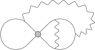
FIG. 12.: A non-4PI vacuum diagram used to calculate the number of particular elements of a vacuum diagram for the topological equation.

A 4PI skeleton is what remains of a 4PI vacuum diagram after one has cut out all the 4-fermion vertices. A vacuum diagram that is not 4PI does in general contain 4PI skeletons by cutting out appropriate subdiagrams, and $N_{skel}$ counts the number of such skeletons. The two gauge exchanges in our example are the only 4PI skeletons, because in each case, if one replaces the rest of the diagram with one 4-fermion vertex, the result is a 4PI diagram. By doing this replacement on any other 4-point subdiagram one finds that there are no other 4PI skeletons. So for our example we have $N_{skel}=2$.

The term, $W_{skel}$, is generated by the sum of all 4PI vacuum diagrams, $V_{4PI}$, where all possible connected 4-point diagrams (the $C$’s) replace the 4-fermion vertices. This gives

$$W_{skel}=V_{4PI}[C,C^{{\dagger}},C_{0},C_{R},C_{L}],$$ (138)

The $C$’s now play the role of 4-fermion vertices, in place of the $J$’s.

The number of articulated quartets, $N_{art}$, counts the number of sets of four fermion lines in a vacuum diagram that one can cut to separate the vacuum diagram into two disconnected parts. There are three such sets in our example. Two sets connect the two gauge exchanges to the rest of the diagram and one set connects the 4-fermion vertex to the rest of the diagram. Thus we have $N_{art}=3$ for our example.

One can generate the term, $W_{art}$, for the set of all vacuum diagrams by closing off the lines of one 4-point diagram by those of another 4-point diagram for all possible connected 4-point diagrams. The result is just the trace over the product of two $C$’s,

$$W_{art}={\rm Tr}\left\{\frac{1}{4}CC^{{\dagger}}+\frac{1}{8}C_{R}^{2}+\frac{1}{8}C_{L}^{2}+\frac{1}{2}C_{0}^{2}\right\}.$$ (139)

The symmetry factors appear as follows: if the term is made of 4-point functions that have identical incoming or outgoing lines then the same factor of $\frac{1}{4}$ which appears in (45) accompanies this term – this is the case for the first three terms in (139); if the two 4-point functions in a term are the same (as in the last three terms of (139)) we need an extra factor of $\frac{1}{2}$.

The third term in (136), $N_{vert}$, is just the number of 4-fermion vertices in a vacuum diagram. Our example contains only one such vertex, so $N_{vert}=1$.

The term, $W_{vert}$, is generated by closing the four lines of all unamputated 4-point diagrams (including disconnected ones) off with the appropriate source $J$, which gives a trace over the product of a $J$ with the Green function ($G$). This generates the five source terms which are removed by the Legendre transform, (46):

$$W_{vert}=\frac{1}{4}JG^{{\dagger}}+\frac{1}{4}J^{{\dagger}}G+J_{0}G_{0}+\frac{1}{4}J_{R}G_{R}+\frac{1}{4}J_{L}G_{L}.$$ (140)

Here we again have factors of $\frac{1}{4}$ which appear due to identical incoming and outgoing lines.

B Pair cycles

A pair cycle is a loop of pairs of fermion lines that connect simple subdiagrams to form a vacuum diagram. (See Fig. 10.) The sum over pair cycles makes up the last three terms in the topological equation (136). The first term in the sum, $\sum 1$, just counts the number of such pair cycles in a vacuum diagram. The next term, $\sum N_{p}$, counts the number of pairs in each pair cycle of the vacuum diagram and the third term in the sum, $\sum N_{pp}$, counts the pairs of pairs in each pair cycle of the diagram. One can see that for 1-cycles and 2-cycles these three terms add up to zero. Therefore it is only for pair cycles with three or more pairs that these terms make a nontrivial contribution to the topological equation. In our example there is only one pair cycle with more than two pairs and it is a 3-cycle. This gives $\sum(1-N_{p}+N_{pp})=1-3+3=1$ for our example. Adding all the numbers for our example according to (136) then gives 1 as it should.

One can define the fourth term in (137), $W_{c}$, as the trace of a power series of simple 4-point functions ($U$’s) with the appropriate symmetry factors. A product of $n$ simple 4-point functions forms a chain of $n$ fermion pairs and the trace of this product closes off the chain into a pair cycle. The next term $W_{p}$ can be generated from the previous one $W_{c}$ by including a parameter $g$ with each $U$ and then taking the derivative with respect to $g$. This counts the number of pairs in each pair cycle, and the second derivative gives twice the number of pairs of pairs. Half of the latter gives the last term, $W_{pp}$. Since the $U$’s can be expressed in terms of the 4-point functions ($C$’s), this procedure leads to the required expressions for the three pair cycle terms. The pair cycles found in our analysis are more complicated than those in [1] because there are several ways to form them due to the distinguished chiralities.

We follow the approach of Sec. V A, which is to divide the different $U$’s into four groups depending on their type of fermion pairs. The pair cycle terms are expressed as

$$H_{Total}=W_{c}-W_{p}+W_{pp}$$ (141)

for each type of fermion pairs. The aim is to find all the different pair cycles by identifying all the $U$’s that can form such cycles. Some $U$’s can form pair cycles on their own. The two pairs of external lines on these $U$’s are compatible, which implies that two of these $U$’s can be interconnected. The other $U$’s have incompatible pairs. Although they cannot form pair cycles on their own, they can be combined with other $U$’s to form a group of simple 4-point functions which can be used to form pair cycles. Such groups of simple 4-point functions are denoted by $M$’s. We shall discuss each of the type of fermion pairs in turn, starting with the simplest case.

1 sd-fermion pairs

The sd-fermion pair has only one simple 4-point function: $U_{s}^{0}$. There are no simple 4-point function groups, $M$’s, for this type of fermion pair. The pair cycle is formed by defining the following quantity:

$$A_{sd}(g)={\rm Tr}\left\{\sum_{n=1}^{\infty}{1\over n}(gU_{s}^{0})^{n}\right\}=-{\rm Tr}\left\{\ln\left(1-gU_{s}^{0}\right)_{s}\right\}.$$ (142)

Setting $g=1$ in (142) one finds the sum of all pair cycles with this type of fermion pair. The number of pairs per cycle is obtained by taking the derivative of $A_{s}^{0}(g)$ with respect to $g$, while a second derivative gives twice the number of pairs of pairs. The sum of pair cycle terms, (141), with sd-fermion pairs are then given by

$$H_{sd} = \left[A_{sd}(g)-{d\over dg}A_{sd}(g)+\frac{1}{2}{d^{2}\over dg^{2}}A_{sd}(g)\right]_{g=1}$$ (143)

$$= {\rm Tr}\left\{-\ln\left(1-U_{s}^{0}\right)_{s}-\left[1-U_{s}^{0}\right]_{s}^{-1}U_{s}^{0}+\frac{1}{2}\left[1-U_{s}^{0}\right]_{s}^{-1}U_{s}^{0}\left[1-U_{s}^{0}\right]_{s}^{-1}U_{s}^{0}\right\}.$$ (144)

From (65) one can show that

$$\left[1-U_{s}^{0}\right]_{s}^{-1}U_{s}^{0}=C_{0}.$$ (145)

Using (145) and (66), (144) becomes

$$H_{sd}={\rm Tr}\left\{\ln\left(1+C_{0}\right)_{s}-C_{0}+\frac{1}{2}C_{0}^{2}\right\}.$$ (146)

This is similar to the result in [1]. The subsequent cases are all treated according to the same steps. For each pair cycle one can define

$$H_{f}=\left[A_{f}(g)-{d\over dg}A_{f}(g)+\frac{1}{2}{d^{2}\over dg^{2}}A_{f}(g)\right]_{g=1},$$ (147)

where the subscript $f$ denotes the specific type of simple 4-point function or simple 4-point function group for that pair cycle. Some algebra necessary to get this expression into a form that only consist of $C$’s.

2 ss-fermion pairs

There are two simple 4-point functions that can directly form pair cycles in the ss-fermion pairs: $U_{s}^{R}$ and $U_{s}^{L}$. There is also a simple 4-point function group that can form pair cycles:

$$M_{s}(g)=\frac{g^{2}}{2}\left[1-\frac{g}{2}U^{R}_{s}\right]_{s}^{-1}U_{s}^{{\dagger}}\left[1-\frac{g}{2}U^{L}_{s}\right]_{s}^{-1}U_{s}=\frac{1}{2}g^{2}R_{s}^{U}(g)U_{s}^{{\dagger}}L_{s}^{U}(g)U_{s}.$$ (148)

Here the pair cycles are formed by

$$A_{ss}(g)={\rm Tr}\left\{\sum_{n=1}^{\infty}{1\over n}\left(\frac{1}{2}M(g)\right)^{n}\right\}=-{\rm Tr}\left\{\ln\left(1-\frac{1}{2}M(g)\right)_{s}\right\},$$ (149)

where $M(g)$ denotes $M_{s}(g)$, $gU_{s}^{R}$ or $gU_{s}^{L}$. The factor of $\frac{1}{2}$ is necessary to remove an overcounting which occurs as a result of the ss-symmetry as discussed in Sec. V A. For $U_{s}^{R}$ and $U_{s}^{L}$ the expressions are only slightly more complicated than in the sd-case. We define separate quantities:

$$H_{s}^{R} = {\rm Tr}\left\{-\ln\left(1-\frac{1}{2}U_{s}^{R}\right)_{s}-\frac{1}{2}\left[1-\frac{1}{2}U_{s}^{R}\right]_{s}^{-1}U_{s}^{R}\right.$$ (151)

$$+\left.\frac{1}{8}\left[1-\frac{1}{2}U_{s}^{R}\right]_{s}^{-1}U_{s}^{R}\left[1-\frac{1}{2}U_{s}^{R}\right]_{s}^{-1}U_{s}^{R}\right\}$$

and

$$H_{s}^{L} = {\rm Tr}\left\{-\ln\left(1-\frac{1}{2}U_{s}^{L}\right)_{s}-\frac{1}{2}\left[1-\frac{1}{2}U_{s}^{L}\right]_{s}^{-1}U_{s}^{L}\right.$$ (153)

$$+\left.\frac{1}{8}\left[1-\frac{1}{2}U_{s}^{L}\right]_{s}^{-1}U_{s}^{L}\left[1-\frac{1}{2}U_{s}^{L}\right]_{s}^{-1}U_{s}^{L}\right\}$$

From (86) and (87) it can be shown that

$$\left[1-\frac{1}{2}U_{s}^{R}\right]_{s}^{-1}U_{s}^{R}=C_{R}-\frac{1}{2}C_{C}^{{\dagger}}L_{s}C_{C}$$ (154)

and

$$\left[1-\frac{1}{2}U_{s}^{L}\right]_{s}^{-1}U_{s}^{L}=C_{L}-\frac{1}{2}C_{C}R_{s}C_{C}^{{\dagger}}.$$ (155)

Using (154) and (89) one finds that (151) becomes

$$H_{s}^{R} = {\rm Tr}\left\{\ln\left(1-\frac{1}{4}C_{C}^{{\dagger}}L_{s}C_{C}R_{s}\right)_{s}+\ln\left(1+\frac{1}{2}C_{R}\right)_{s}-\frac{1}{2}\left(C_{R}-\frac{1}{2}C_{C}^{{\dagger}}L_{s}C_{C}\right)\right.$$ (157)

$$+\left.\frac{1}{8}\left(C_{R}-\frac{1}{2}C_{C}^{{\dagger}}L_{s}C_{C}\right)^{2}\right\}.$$

Similarly, from (155) and (90), (153) becomes

$$H_{s}^{L} = {\rm Tr}\left\{\ln\left(1-\frac{1}{4}C_{C}R_{s}C_{C}^{{\dagger}}L_{s}\right)_{s}+\ln\left(1+\frac{1}{2}C_{L}\right)_{s}-\frac{1}{2}\left(C_{L}-\frac{1}{2}C_{C}R_{s}C_{C}^{{\dagger}}\right)\right.$$ (159)

$$+\left.\frac{1}{8}\left(C_{L}-\frac{1}{2}C_{C}R_{s}C_{C}^{{\dagger}}\right)^{2}\right\}.$$

Due to the intricate $g$-dependence in (148) the pair cycle expression that contains $M_{s}$ is more complicated:

$$H_{s}^{M} = {\rm Tr}\left\{-\ln\left(1-\frac{1}{4}R_{s}^{U}U_{s}^{{\dagger}}L_{s}^{U}U_{s}\right)_{s}\right.$$ (163)

$$-\frac{1}{2}\left[1-\frac{1}{4}R_{s}^{U}U_{s}^{{\dagger}}L_{s}^{U}U_{s}\right]_{s}^{-1}\left((R_{s}^{U})^{2}U_{s}^{{\dagger}}L_{s}^{U}U_{s}+R_{s}^{U}U_{s}^{{\dagger}}(L_{s}^{U})^{2}U_{s}\right)$$

$$+\frac{1}{4}\left[1-\frac{1}{4}R_{s}^{U}U_{s}^{{\dagger}}L_{s}^{U}U_{s}\right]_{s}^{-1}\left((R_{s}^{U})^{3}U_{s}^{{\dagger}}L_{s}^{U}U_{s}+(R_{s}^{U})^{2}U_{s}^{{\dagger}}(L_{s}^{U})^{2}U_{s}+R_{s}^{U}U_{s}^{{\dagger}}(L_{s}^{U})^{3}U_{s}\right)$$

$$+\left.\frac{1}{2}\left(\frac{1}{4}\left[1-\frac{1}{4}R_{s}^{U}U_{s}^{{\dagger}}L_{s}^{U}U_{s}\right]_{s}^{-1}\left((R_{s}^{U})^{2}U_{s}^{{\dagger}}L_{s}^{U}U_{s}+R_{s}^{U}U_{s}^{{\dagger}}(L_{s}^{U})^{2}U_{s}\right)\right)^{2}\right\}.$$

Here we used the identity

$${d\over dg}B=\frac{1}{g}\left(B^{2}-B\right),$$ (164)

where $B=[1-gA]^{-1}$ for a 4-point function, $A$. Using the identities in (V B 2) and (93), one can show that

$$H_{s}^{M} = {\rm Tr}\left\{-\ln\left(1-\frac{1}{4}C_{C}R_{s}C_{C}^{{\dagger}}L_{s}\right)_{s}+\frac{1}{8}C_{C}C_{R}C_{C}^{{\dagger}}L_{s}+\frac{1}{8}C_{C}R_{s}C_{C}^{{\dagger}}C_{L}+\frac{1}{4}C_{C}^{{\dagger}}C_{C}\right.$$ (166)

$$-\left.\frac{1}{4}C_{C}C_{C}^{{\dagger}}L_{s}-\frac{1}{4}C_{C}R_{s}C_{C}^{{\dagger}}-\frac{1}{32}C_{C}C_{C}^{{\dagger}}L_{s}C_{C}C_{C}^{{\dagger}}L_{s}-\frac{1}{32}C_{C}R_{s}C_{C}^{{\dagger}}C_{C}R_{s}C_{C}^{{\dagger}}\right\}.$$

Now one can add all the $H$’s for the ss-fermion pairs:

$$H_{ss} = H_{s}^{M}+H_{s}^{R}+H_{s}^{L}$$ (167)

$$= {\rm Tr}\left\{\ln\left(1-\frac{1}{4}C_{C}R_{s}C_{C}^{{\dagger}}L_{s}\right)_{s}+\ln\left(1+\frac{1}{2}C_{R}\right)_{s}+\ln\left(1+\frac{1}{2}C_{L}\right)_{s}\right.$$ (169)

$$-\left.\frac{1}{2}C_{R}-\frac{1}{2}C_{L}+\frac{1}{8}C_{R}^{2}+\frac{1}{8}C_{L}^{2}+\frac{1}{4}C_{C}C_{C}^{{\dagger}}\right\}.$$

The resulting expression is relatively simple thanks to extensive cancellations among the different $H$’s.

The remaining two types of fermion pairs follow exactly the same procedure and the expressions that are obtained are also very similar to these. We quote all the relevant expressions without unnecessary discussion.

3 ds-fermion pairs

The two simple 4-point functions that can directly form pair cycles in the ds-fermion pairs are $U_{d}^{R}$ and $U_{d}^{L}$ and the simple 4-point function group that can form pair cycles is

$$M_{ds}(g)=g^{2}[1-gU^{R}_{d}]_{d}^{-1}U_{d}^{\prime}[1-gU^{L}_{d}]_{d}^{-1}U_{d}^{\prime}=g^{2}R_{d}^{U}U_{d}^{\prime}L_{d}^{U}U_{d}^{\prime}.$$ (170)

The pair cycles are formed by

$$A_{d}(g)=\frac{1}{2}{\rm Tr}\left\{\sum_{n=1}^{\infty}{1\over n}M(g)^{n}\right\}=-\frac{1}{2}{\rm Tr}\left\{\ln\left(1-M(g)\right)_{d}\right\}$$ (171)

where $M(g)$ denotes $M_{ds}(g)$, $gU_{d}^{R}$ or $gU_{d}^{L}$. There is a symmetry with respect to a front-to-back transformation of these pair cycles. The factor of $\frac{1}{2}$ is necessary to remove the overcounting which occurs as a result of this symmetry. For $U_{d}^{R}$ and $U_{d}^{L}$ we have the following expressions for (147), using (171):

$$H_{d}^{R} = {\rm Tr}\left\{-\frac{1}{2}\ln\left(1-U_{d}^{R}\right)_{d}-\frac{1}{2}\left[1-U_{d}^{R}\right]_{d}^{-1}U_{d}^{R}\right.$$ (173)

$$+\left.\frac{1}{4}\left[1-U_{d}^{R}\right]_{d}^{-1}U_{d}^{R}\left[1-U_{d}^{R}\right]_{d}^{-1}U_{d}^{R}\right\}$$

and

$$H_{d}^{L} = {\rm Tr}\left\{-\frac{1}{2}\ln\left(1-U_{d}^{L}\right)_{d}-\frac{1}{2}\left[1-U_{d}^{L}\right]_{d}^{-1}U_{d}^{L}\right.$$ (175)

$$+\left.\frac{1}{4}\left[1-U_{d}^{L}\right]_{d}^{-1}U_{d}^{L}\left[1-U_{d}^{L}\right]_{d}^{-1}U_{d}^{L}\right\}.$$

One can show, from (97) and (98), that

$$\left[1-U_{d}^{R}\right]_{d}^{-1}U_{d}^{R}=C_{R}-C_{0}LC_{0}$$ (176)

and

$$\left[1-U_{d}^{L}\right]_{d}^{-1}U_{d}^{L}=C_{L}-C_{0}RC_{0}.$$ (177)

Using (176) and (100) one finds that (173) becomes

$$H_{d}^{R} = {\rm Tr}\left\{\frac{1}{2}\ln\left(1-C_{0}LC_{0}R\right)_{d}+\frac{1}{2}\ln\left(1+C_{R}\right)_{d}-\frac{1}{2}\left(C_{R}-C_{0}LC_{0}\right)\right.$$ (179)

$$+\left.\frac{1}{4}\left(C_{R}-C_{0}LC_{0}\right)^{2}\right\}.$$

Similarly, from (177) and (101), (175) becomes

$$H_{d}^{L} = {\rm Tr}\left\{\frac{1}{2}\ln\left(1-C_{0}RC_{0}L\right)_{d}+\frac{1}{2}\ln\left(1+C_{L}\right)_{d}-\frac{1}{2}\left(C_{L}-C_{0}RC_{0}\right)\right.$$ (181)

$$+\left.\frac{1}{4}\left(C_{L}-C_{0}RC_{0}\right)^{2}\right\}.$$

The pair cycle expression that contains $M_{ds}$ is:

$$H_{ds}^{M} = {\rm Tr}\left\{-\frac{1}{2}\ln\left(1-R_{d}^{U}U_{d}^{\prime}L_{d}^{U}U_{d}^{\prime}\right)_{d}\right.$$ (185)

$$-\left[1-R_{d}^{U}U_{d}^{\prime}L_{d}^{U}U_{d}^{\prime}\right]_{d}^{-1}\left((R_{d}^{U})^{2}U_{d}^{\prime}L_{d}^{U}U_{d}^{\prime}+R_{d}^{U}U_{d}^{\prime}(L_{d}^{U})^{2}U_{d}^{\prime}\right)$$

$$+\frac{1}{2}\left[1-R_{d}^{U}U_{d}^{\prime}L_{d}^{U}U_{d}^{\prime}\right]_{d}^{-1}\left((R_{d}^{U})^{3}U_{d}^{\prime}L_{d}^{U}U_{d}^{\prime}+(R_{d}^{U})^{2}U_{d}^{\prime}(L_{d}^{U})^{2}U_{d}^{\prime}+R_{d}^{U}U_{d}^{\prime}(L_{d}^{U})^{3}U_{d}^{\prime}\right)$$

$$+\left.\frac{1}{4}\left(\left[1-R_{d}^{U}U_{d}^{\prime}L_{d}^{U}U_{d}^{\prime}\right]_{d}^{-1}\left((R_{d}^{U})^{2}U_{d}^{\prime}L_{d}^{U}U_{d}^{\prime}+R_{d}^{U}U_{d}^{\prime}(L_{d}^{U})^{2}U_{d}^{\prime}\right)\right)^{2}\right\},$$

where we again used the identity in (164). The identities in (V B 2) lead to

$$H_{d}^{M} = {\rm Tr}\left\{-\frac{1}{2}\ln\left(1-C_{0}LC_{0}R\right)_{d}+\frac{1}{2}C_{0}C_{R}C_{0}L+\frac{1}{2}C_{0}RC_{0}C_{L}+\frac{1}{2}C_{0}^{2}\right.$$ (187)

$$-\left.\frac{1}{2}C_{0}C_{0}L-\frac{1}{2}C_{0}RC_{0}-\frac{1}{4}C_{0}C_{0}LC_{0}C_{0}L-\frac{1}{4}C_{0}RC_{0}C_{0}RC_{0}\right\}.$$

Now one can add all the $H$’s for the sd-fermion pairs:

$$H_{ds} = H_{ds}^{M}+H_{d}^{R}+H_{d}^{L}$$ (188)

$$= {\rm Tr}\left\{\frac{1}{2}\ln\left(1-C_{0}LC_{0}R\right)_{d}+\frac{1}{2}\ln\left(1+C_{R}\right)_{d}+\frac{1}{2}\ln\left(1+C_{L}\right)_{d}\right.$$ (190)

$$-\left.\frac{1}{2}C_{R}-\frac{1}{2}C_{L}+\frac{1}{4}C_{R}^{2}+\frac{1}{4}C_{L}^{2}+\frac{1}{2}C_{0}^{2}\right\}.$$

Here too we have a relatively simple expression as a result of cancellations among the different $H$’s.

4 dd-fermion pairs

There is only one simple 4-point function, $U_{d}^{0}$, which can directly form a pair cycle in the dd-fermion pairs. The simple 4-point function group for this type of fermion pairs is

$$M_{dd}(g)=g^{2}[1-gU_{d}^{0}]_{d}^{-1}U_{d}^{{\dagger}}[1-gU_{d}^{0}]_{d}^{-1}U_{d}=g^{2}BU_{d}^{{\dagger}}BU_{d}.$$ (191)

Because $U_{d}^{0}$ looks different under a front-to-back transformation we shall use it twice. These two pair cycles are then related through a back-to-front transformation and each must be multiplied by $\frac{1}{2}$. The pair cycle for the simple 4-point function group of (191) has a front-to-back symmetry. The pair cycles are therefore formed by the expression in (171) where $M(g)$ denotes $M_{dd}(g)$ or $gU_{d}^{0}$.

Substituting $U_{d}^{0}$ into (147), using (171), gives

$$H_{d}^{0} = {\rm Tr}\left\{-\frac{1}{2}\ln\left(1-U_{d}^{0}\right)_{d}-\frac{1}{2}\left[1-U_{d}^{0}\right]_{d}^{-1}U_{d}^{0}\right.$$ (193)

$$+\left.\frac{1}{4}\left[1-U_{d}^{0}\right]_{d}^{-1}U_{d}^{0}\left[1-U_{d}^{0}\right]_{d}^{-1}U_{d}^{0}\right\}.$$

From this expression one can use two different sets of expressions to get two different results which are related by a back-to-front transformation. First one can use (106) and (107), to show that

$$\left[1-U_{d}^{0}\right]_{d}^{-1}U_{d}^{0}=C_{0}-C_{C}^{{\dagger}}ZC_{C}$$ (194)

or one can use (105) and (108), to show that

$$\left[1-U_{d}^{0}\right]_{d}^{-1}U_{d}^{0}=C_{0}-C_{C}ZC_{C}^{{\dagger}}.$$ (195)

Substituting (194) and (111) into (193) one finds

$$H_{d}^{0} = {\rm Tr}\left\{\frac{1}{2}\ln\left(1-C_{C}^{{\dagger}}ZC_{C}Z\right)_{d}+\frac{1}{2}\ln\left(1+C_{0}\right)_{d}-\frac{1}{2}\left(C_{0}-C_{C}^{{\dagger}}ZC_{C}\right)\right.$$ (197)

$$+\left.\frac{1}{4}\left(C_{0}-C_{C}^{{\dagger}}ZC_{C}\right)^{2}\right\}$$

and substituting (195) and (110) into (193) one finds

$$H_{d}^{0{\dagger}} = {\rm Tr}\left\{\frac{1}{2}\ln\left(1-C_{C}ZC_{C}^{{\dagger}}Z\right)_{d}+\frac{1}{2}\ln\left(1+C_{0}\right)_{d}-\frac{1}{2}\left(C_{0}-C_{C}ZC_{C}^{{\dagger}}\right)\right.$$ (199)

$$+\left.\frac{1}{4}\left(C_{0}-C_{C}ZC_{C}^{{\dagger}}\right)^{2}\right\},$$

where we placed a ${\dagger}$ on the $H$ in the latter expression to show that the chiralities on the fermion lines are interchanged. The pair cycle terms that contain $M_{ds}$ are:

$$H_{dd}^{M} = {\rm Tr}\left\{-\frac{1}{2}\ln\left(1-BU_{d}^{{\dagger}}BU_{d}\right)_{d}-\left[1-BU_{d}^{{\dagger}}BU_{d}\right]_{d}^{-1}\left(B^{2}U_{d}^{{\dagger}}BU_{d}+BU_{d}^{{\dagger}}B^{2}U_{d}\right)\right.$$ (202)

$$+\frac{1}{2}\left[1-BU_{d}^{{\dagger}}BU_{d}\right]_{d}^{-1}\left(B^{3}U_{d}^{{\dagger}}BU_{d}+B^{2}U_{d}^{{\dagger}}B^{2}U_{d}+BU_{d}^{{\dagger}}B^{3}U_{d}\right)$$

$$+\left.\frac{1}{4}\left(\left[BU^{{\dagger}}_{d}BU_{d}\right]_{d}^{-1}\left(B^{2}U_{d}^{{\dagger}}BU_{d}+BU_{d}^{{\dagger}}B^{2}U_{d}\right)\right)^{2}\right\},$$

where we used the identity in (164). The expressions in (V B 2) then gives

$$H_{dd}^{M} = {\rm Tr}\left\{-\frac{1}{2}\ln\left(1-C_{C}ZC_{C}^{{\dagger}}Z\right)_{d}+\frac{1}{2}C_{C}C_{0}C_{C}^{{\dagger}}Z+\frac{1}{2}C_{C}ZC_{C}^{{\dagger}}C_{0}+\frac{1}{2}C_{C}C_{C}^{{\dagger}}\right.$$ (204)

$$-\left.\frac{1}{2}C_{C}C_{C}^{{\dagger}}Z-\frac{1}{2}C_{C}ZC_{C}^{{\dagger}}-\frac{1}{4}C_{C}C_{C}^{{\dagger}}ZC_{C}C_{C}^{{\dagger}}Z-\frac{1}{4}C_{C}ZC_{C}^{{\dagger}}C_{C}ZC_{C}^{{\dagger}}\right\}.$$

Adding all the $H$’s for the dd-fermion pairs, one finds

$$H_{dd} = H_{dd}^{M}+H_{d}^{0}+H_{d}^{0{\dagger}}$$ (205)

$$= {\rm Tr}\left\{\frac{1}{2}\ln\left(1-C_{C}ZC_{C}^{{\dagger}}Z\right)_{d}+\ln\left(1+C_{0}\right)_{d}-C_{0}+\frac{1}{2}C_{0}^{2}+\frac{1}{2}C_{C}C_{C}^{{\dagger}}\right\}.$$ (206)

C The effective action

Now one can construct the expression for the pair cycle terms of the effective action (141) by adding the expressions in (146), (169), (190) and (206)

$$H_{Total} = H_{sd}+H_{ss}+H_{ds}+H_{dd}$$ (207)

$$= {\rm Tr}\left\{\ln\left(1-\frac{1}{4}R_{s}C_{C}^{{\dagger}}L_{s}C_{C}\right)_{s}+\ln\left(1+\frac{1}{2}C_{R}\right)_{s}+\ln\left(1+\frac{1}{2}C_{L}\right)_{s}\right.$$ (211)

$$+\frac{1}{2}\ln\left(1-RC_{0}LC_{0}\right)_{d}+\frac{1}{2}\ln\left(1+C_{R}\right)_{d}+\frac{1}{2}\ln\left(1+C_{L}\right)_{d}+\ln\left(1+C_{0}\right)_{d}$$

$$+\frac{1}{2}\ln\left(1-ZC_{C}^{{\dagger}}ZC_{C}\right)_{d}+\ln(1+C_{0})_{s}-C_{R}-C_{L}-2C_{0}$$

$$\left.+\frac{3}{4}C_{C}C_{C}^{{\dagger}}+\frac{3}{2}C_{0}^{2}+\frac{3}{8}C_{R}^{2}+\frac{3}{8}C_{L}^{2}\right\}.$$

One can then combine the different parts in (138), (139), (140) and (211) to construct the generating functional, $W$ – i.e. the set of all connected vacuum diagrams. Next one can perform the Legendre transform, (46), which removes (140) to produce the expression of the full effective action. With all the explicit $J$-dependence removed, the effective action becomes a functional of the 4-point functions:

$$\Gamma = W_{c}-W_{p}+W_{pp}-W_{art}+W_{skel}$$ (212)

$$= {\rm Tr}\left\{\ln\left(1-\frac{1}{4}R_{s}C^{{\dagger}}L_{s}C\right)_{s}+\ln\left(1+\frac{1}{2}C_{R}\right)_{s}+\ln\left(1+\frac{1}{2}C_{L}\right)_{s}+\ln(1+C_{0})_{s}\right.$$ (216)

$$+\frac{1}{2}\ln\left(1-RC_{0}LC_{0}\right)_{d}+\frac{1}{2}\ln\left(1+C_{R}\right)_{d}+\frac{1}{2}\ln\left(1+C_{L}\right)_{d}+\ln\left(1+C_{0}\right)_{d}$$

$$+\frac{1}{2}\ln\left(1-ZC^{{\dagger}}ZC\right)_{d}-C_{R}-C_{L}-2C_{0}$$

$$\left.+\frac{1}{2}CC^{{\dagger}}+C_{0}^{2}+\frac{1}{4}C_{R}^{2}+\frac{1}{4}C_{L}^{2}\right\}+V_{4PI}[C,C^{{\dagger}},C_{0},C_{R},C_{L}].$$

This result for the effective action is the main result of our analysis. It can be applied to arbitrary models, and it provides the means to determine which solution of the gap equations of Sec. V represents the true vacuum of the theory.

Here we want to remark on the large $N_{c}$ expansion of this effective action, which is discussed in Sec. II. When such an expansion is made and only the leading terms are retained, one notes that $H_{ss}$ in (169) and $H_{sd}$ in (146) are suppressed because their fermion loops cannot form color loops. Next one notes that $H_{ds}$ in (190) and $H_{dd}$ in (206) decouple from each other because they do not share the same $C$’s. (Each of $H_{ds}$ and $H_{dd}$ contain one of the respective color structures of $C_{0}$ – see discussion below (20).) This leads to the two decoupled effective actions which are presented in (22) and (24).

VII Obtaining gap equations from the effective action

The gap equations for the 4-point functions (V D) are obtained by taking the functional derivatives of the effective action (216), as in (52), and then amputating the result. A key step in this process is to take the functional derivatives of the pair cycle terms which are provided in (146), (169), (190) and (206). It is necessary to take special care of the assignments of external lines which result from these functional derivatives. For the case of $C_{0}$ this is just

$${\delta C_{0}(1,2,3,4)\over\delta C_{0}(a,b,c,d)}=\delta_{a}^{1}\delta_{b}^{2}\delta_{c}^{3}\delta_{d}^{4},$$ (217)

where we use $1,2,3,4$ and $a,b,c,d$ to distinguish external fermion lines. For the other four cases, $C_{C}$, $C_{C}^{{\dagger}}$, $C_{R}$ and $C_{L}$, we have

$${\delta C(1,2,3,4)\over\delta C(a,b,c,d)}=[\delta_{a}^{1}\delta_{c}^{3}+\delta_{c}^{1}\delta_{a}^{3}][\delta_{b}^{2}\delta_{d}^{4}+\delta_{d}^{2}\delta_{b}^{4}].$$ (218)

The latter functional derivative gives rise to four terms. Often these four terms may be related to each other through some interchanges of external lines. These transformations are defined in (9).

Next we calculate the functional derivatives of the $H$’s in (146), (169), (190) and (206) with respect to $C_{0}$, $C_{C}^{{\dagger}}$ and $C_{R}$. Those of $C_{C}$ and $C_{L}$ are related to these in an obvious way. In each case we shall find that the functional derivative of the pair cycles of a specific type of fermion pairs with respect to a specific 4-point function reproduces a specific $T$ (or more than one if they are related by one of the above transformations).

We start with $C_{0}$. Only the pair cycles with the sd-, ds- and dd-fermion pairs depend on $C_{0}$. Their functional derivatives are

$$\left.{\delta H_{sd}\over\delta C_{0}}\right|_{amp}=\left[1+C_{0}\right]_{s}^{-1}-1+C_{0}=T_{s}^{0};$$ (219)

$$\left.{\delta H_{ds}\over\delta C_{0}}\right|_{amp} = \frac{1}{2}\left[1-RC_{0}LC_{0}\right]_{d}^{-1}\left(-RC_{0}L\right)+\frac{1}{2}\left(-LC_{0}\left[1-RC_{0}LC_{0}\right]_{d}^{-1}R\right)^{RF}+C_{0}$$ (220)

$$= C_{0}-RC_{0}L\left[1-C_{0}RC_{0}L\right]_{d}^{-1}=T_{d}^{\prime};$$ (221)

$$\left.{\delta H_{dd}\over\delta C_{0}}\right|_{amp} = \frac{1}{2}\left(Z\left[1-C_{C}ZC_{C}^{{\dagger}}Z\right]_{d}^{-1}C_{C}ZC_{C}^{{\dagger}}Z\right)+\frac{1}{2}\left(Z\left[1-C_{C}^{{\dagger}}ZC_{C}Z\right]_{d}^{-1}C_{C}^{{\dagger}}ZC_{C}Z\right)^{RF}$$ (223)

$$+\left[1+C_{0}\right]_{d}^{-1}-1+C_{0}$$

$$= C_{0}+Z\left[1-C_{C}ZC_{C}^{{\dagger}}Z\right]_{d}^{-1}-1=T_{d}^{0}.$$ (224)

The $RF$ transformations shown in (221) and (224) are equal to the $RF$ transformations applied to each individual object in reversed order in each of the terms. This reproduces the three $T$’s that appear in the gap equation for $C_{0}$, (67), (120) and (128). Next we consider $C_{C}^{{\dagger}}$. Only the pair cycles in the ss- and dd-fermion pairs depend on $C_{C}^{{\dagger}}$:

$$\left.{\delta H_{ss}\over\delta C_{C}^{{\dagger}}}\right|_{amp} = \left[1-\frac{1}{4}L_{s}C_{C}R_{s}C_{C}^{{\dagger}}\right]_{s}^{-1}\left(-\frac{1}{4}L_{s}C_{C}R_{s}\right)\left(\times 4\right)+\frac{1}{4}C_{C}\left(\times 4\right)$$ (225)

$$= C_{C}-L_{s}C_{C}R_{s}\left[1-\frac{1}{4}C_{C}^{{\dagger}}L_{s}C_{C}R_{s}\right]_{s}^{-1}=T_{s};$$ (226)

$$\left.{\delta H_{dd}\over\delta C_{C}^{{\dagger}}}\right|_{amp} = \frac{1}{2}\left[1-ZC_{C}ZC_{C}^{{\dagger}}\right]_{d}^{-1}\left(-ZC_{C}Z\right)\left(1+1^{RF}+1^{T}+1^{RFT}\right)$$ (228)

$$+\frac{1}{2}C\left(1+1^{RF}+1^{T}+1^{RFT}\right)$$

$$= \left(C_{C}-ZC_{C}Z\left[1-C_{C}^{{\dagger}}ZC_{C}Z\right]_{d}^{-1}\right)\left(1+1^{T}\right)=T_{d}+\left(T_{d}\right)^{T}.$$ (229)

The $(\times 4)$ comes from the ss-symmetry which generates four identical terms. The $(1+1^{RF}+1^{T}+1^{RFT})$ denotes different exchanges of external lines. Because the diagram is symmetric under the combined $RF$-transformation, the expression reduces to the final expression with a factor of 2. Thus we reproduce the three $T$’s which appear in the gap equation for $C_{C}$, (115) and (125). The gap equation for $C_{C}^{{\dagger}}$ is quite similar. One merely interchanges the chiralities to get the necessary expressions. For $C_{R}$ only the ss- and ds-fermion pairs need to be considered:

$$\left.{\delta H_{ss}\over\delta C_{R}}\right|_{amp} = \left(-\frac{1}{2}R_{s}\left[1-\frac{1}{4}C_{C}^{{\dagger}}L_{s}C_{C}R_{s}\right]_{s}^{-1}\left(-\frac{1}{4}C_{C}^{{\dagger}}L_{s}C_{C}R_{s}\right)+\frac{1}{2}R_{s}-\frac{1}{2}+\frac{1}{4}C_{R}\right)\left(\times 4\right)$$ (230)

$$= C_{R}+2R_{s}\left[1-\frac{1}{4}C_{C}^{{\dagger}}L_{s}C_{C}R_{s}\right]_{s}^{-1}-2=T_{s}^{R};$$ (231)

$$\left.{\delta H_{ds}\over\delta C_{R}}\right|_{amp} = \left(-\frac{1}{2}R\left[1-C_{0}LC_{0}R\right]_{d}^{-1}\left(-C_{0}LC_{0}R\right)+\frac{1}{2}R\right.$$ (233)

$$-\left.\frac{1}{2}+\frac{1}{2}C_{R}\right)\left(1+1^{RF}+1^{T}+1^{RFT}\right)$$

$$= \left(C_{R}+R\left[1-C_{0}LC_{0}R\right]_{d}^{-1}-1\right)\left(1+1^{T}\right)=T_{d}^{R}+\left(T_{d}^{R}\right)^{T}.$$ (234)

So finally we reproduced the three $T$’s which appear in the $C_{R}$ gap equation – (117) and (122). Those for $C_{L}$ would be identical apart from replacing $R$ with $L$.

Next we find the functional derivatives of $W_{art}$ with respect to the various 4-point functions. (Amputation is implied in all of the following.)

$${\delta W_{art}\over\delta C_{C}^{{\dagger}}}=C_{C},~{}~{}~{}{\delta W_{art}\over\delta C_{C}}=C_{C}^{{\dagger}},~{}~{}~{}{\delta W_{art}\over\delta C_{0}}=C_{0},~{}~{}~{}{\delta W_{art}\over\delta C_{R}}=C_{R}~{}~{}~{}{\rm and}~{}~{}~{}{\delta W_{art}\over\delta C_{L}}=C_{L}.$$ (235)

Finally the functional derivatives of $W_{skel}$ with respect to the various 4-point functions gives rise to the 4PI 4-point diagrams which appear as the $K$-terms in the gap equations:

$${\delta W_{skel}\over\delta C_{C}^{{\dagger}}}=K_{C},~{}~{}~{}{\delta W_{skel}\over\delta C_{C}}=K_{C}^{{\dagger}},~{}~{}~{}{\delta W_{skel}\over\delta C_{0}}=K_{0},~{}~{}~{}{\delta W_{skel}\over\delta C_{R}}=K_{R}~{}~{}~{}{\rm and}~{}~{}~{}{\delta W_{skel}\over\delta C_{L}}=K_{L}.$$ (236)

Collecting the different terms for each specific 4-point function according to (137), using (141) and the first line of (211), one reproduces the gap equations exactly as in (V D).

REFERENCES

- [1] C. de Dominicis and P. C. Martin, J. Math. Phys. 5, 14 and 31 (1964).
- [2] J. M. Cornwell, R. Jackiw and E. Tomboulis, Phys. Rev. D10 2428 (1974).
- [3] G. ’t Hooft, Phys. Rev. D14, 3432 (1976); Phys. Rep. 142, 357 (1986).
- [4] See for example: M. E. Peskin, “Chiral symmetry and chiral symmetry breaking”, Lectures for the Les Houches Summer School of Theoretical Physics, (1982)
- [5] B. Holdom and G. Triantaphyllou, Phys. Rev. D51 7124 (1995).
- [6] P. Maris and Q. Wang, Phys. Rev. D53 4650 (1997), hep-ph/9511403.