March 15, 2024 BI-TP 99/20         
ESI-733-1999         

ANOMALOUS CURRENTS AND 
GLUON CONDENSATES IN QCD 
AT FINITE TEMPERATURE

David E. Miller^1,2

¹ Fakultät für Physik, Universität Bielefeld, Postfach 100131,

D-33501 Bielefeld, Germany

² Department of Physics, Pennsylvania State University, Hazleton Campus,

Hazleton, Pennsylvania 18201, USA (permanent address)

Abstract

After a short description of the currents coming from the known conservation laws in classical physics, we look at some further cases which arise after quantization in relation to quantum chromodynamics (QCD) at finite temperature. In these cases, however, some basic changes appear with the anomalies. First we go into the relationship between the trace of the energy momentum tensor and the gluon condensates at finite temperatures. Using the recent numerical data from the simulations of lattice gauge theory we present the computational evaluations for the gluon condensates at finite temperatures. Thereafter we discuss the effects of chiral symmetry breaking and its restoration at finite temperature through the chiral phase transition. In this context we investigate the properties of the gluon condensate in the presence of massive dynamical quarks using the numerical data. Finally we put together these results with a discussion of the various anomalous currents and their relationship to our findings here.

PACS numbers: 12.38Aw, 11.15Ha, 12.38Mh, 11.40.Dw  

1 Introduction

It is well known that the Maxwell Equations are invariant under the ten generators of the Lorentz Group. This property may be expressed by means of the conservation laws for the terms corresponding to the energy-momentum (4 terms) and the angular momentum (6 terms). This was the understanding already at the founding of the special theory of relativity [1]. Not long thereafter Bateman [2] pointed out that electromagnetism in vacuuo had a much greater invariance under the fifteen generator conformal group. Some of the consequences of this were later pointed out in a work of Bessel-Hagen [3], which came out of an investigation of the conservation laws due to Noether [4] in both mechanics and electrodynamics with special attention to the corresponding currents. This work [3] made a careful analysis of the conformal group and its realization in the additional currents known as the special conformal and dilatation currents, which appear in addition to those of the conserved energy, momentum and angular momentum. Furthermore, it was then [3] realized that the special conformal (4 terms) and the dilatation (1 term) currents are not conserved when massive particles are present. This fact may be expressed by the presence of a trace in the energy momentum tensor. However, Bessel-Hagen then proceeded to set this trace to zero in order to get the sought after conservation equations. This procedure is clearly valid in classical electrodynamics when no massive particles are present. The obtained conservation laws represent all the currents invariant under the full conformal group in Minkowski space-time. This is historically the classically expected situation for a pure gauge invariant field theory.  
About one half a century ago Steinberger as well as Fukuda and Miyamoto studied the electromagnetic decay of the neutral pion into two photons $\pi^{0}\leavevmode\nobreak\ \rightarrow\leavevmode\nobreak\ 2\gamma$. They regarded this process as going over to a virtual pair of proton and antiproton written in the form of the now famous triangle diagram where $\pi^{0}\leavevmode\nobreak\ \rightarrow\leavevmode\nobreak\ {{p}{\bar{p}}}\leavevmode\nobreak\ \rightarrow\leavevmode\nobreak\ 2\gamma$ . This brought about a number of studies of related ideas especially that of Schwinger who pointed out that the conservation of the axial current $J^{\mu}_{5}$ given by $\bar{\psi}{\gamma^{\mu}}{\gamma_{5}}\psi$ in QED is not upheld when the current is properly regularized. This fact is stated by the divergence of this axial current in the equation

$$\partial_{\mu}J^{\mu}_{5}\leavevmode\nobreak\ =\leavevmode\nobreak\ J_{5}\leavevmode\nobreak\ +{{{e^{2}}k}\over{8\pi^{2}}}{{\bar{F}^{\mu\nu}}F_{\mu\nu}},$$ (1.1)

where $J_{5}$ is $2imP$ with $P$ as $\bar{\psi}{\gamma_{5}}\psi$ the expected pseudoscalar part of the divergence relating to the particle mass $m$, k is a constant containing some numerical factors like $\hbar$ and $F^{\mu\nu}$ and ${\bar{F}^{\mu\nu}}$ are the electromagnetic field strength tensor and its dual. This result was later rediscovered in 1969 independenly by Adler in spinor electrodynamics and Bell and Jackiw [5] for the $\sigma$ model. Their results were very similar to the above form in (1.1). A discussion of the axial current anomaly is found in the literature [6, 7]. We will look into the properties of the axial currents in relation to the breaking of chiral symmetry in QCD and its restoration at very high temperatures.  
Now we want to look at these currents to discuss them in relation to the physics arising in the presence of strong interactions. We shall assume a local conservation of energy and momentum under the strong interaction. During the course of this work we shall see how the unconserved currents in QCD at finite temperature come to provide particular differential forms. First we look at the dilatation current $D^{\mu}$ and the four special conformal currents $K^{\mu\alpha}$. We begin with the equation for $D^{\mu}(x)$ which is just the product $x_{\alpha}T^{\mu\alpha}$ of the displacement four vector $x^{\mu}$ and the energy momentum tensor $T^{\mu\nu}$ whose four-divergence gives after renormalization just the trace of the energy- momentum tensor $T^{\mu}_{\mu}$ as follows:

$$\partial_{\mu}D^{\mu}\leavevmode\nobreak\ =\leavevmode\nobreak\ T^{\mu}_{\mu}.$$ (1.2)

A similar equation can be written for the divergence of the special conformal currents

$$\partial_{\mu}K^{\mu\alpha}\leavevmode\nobreak\ =\leavevmode\nobreak\ 2{x^{\alpha}}T^{\mu}_{\mu},$$ (1.3)

where the special conformal currents $K^{\mu\alpha}$ are given by

$$K^{\mu\alpha}\leavevmode\nobreak\ =\leavevmode\nobreak\ (2{x^{\alpha}}{x_{\nu}}\leavevmode\nobreak\ -\leavevmode\nobreak\ g^{\alpha}_{\nu})T^{\mu\nu}.$$ (1.4)

Prior to around 1970 it was generally supposed that the finiteness of $T^{\mu}_{\mu}$ related only to known masses. The renormalization of the nonabelian field theories and the study of the renormalization group equations (Callan-Symanzik equations) brought new attention to the problem. Now this brings us to the point of actually considering what is new in QCD at finite temperatures. Furthermore, we also want to know why all the conservation laws of classical electromagnetism do not fulfill our expectations. The simple answer to these questions lie in the process of renormalization of the quantum field theory, which acts as a scale setter. We shall also discuss the chiral anomaly both for its historical role as well as its role in the presence of dynamical quarks.  
In the next section we shall first discuss the consequences for the gluon condensate at finite temperature. Thereafter we use the results of numerical simulations for the pure gauge theories [8, 9]. The essential relationship for these calculations is the trace anomaly which arises directly from the scale variance of QCD. It relates the trace of the energy momentum tensor to the square of the gluon field strenths through the renormalization group beta function. Here we shall expand upon the approach investigated in [10], for which the consequences of the new finite temperature lattice data for $SU(N_{c})$ gauge theory for the gluon condensate [11] have been presented. After this we shall look into some of the properties of the chiral condensate at finite temperature in relation to the axial anomaly in QCD, which relates to the presence of the quark condensates at finite temperatures. At this point we will consider from the numerical results the properties of the gluon condensate in the presence of dynamical quarks. Then we mention some of the properties of the anomalous currents at finite temperature in terms of the related differential forms to which we ascribe a certain physical meaning. Finally we conclude this work with a brief discussion of a three dynamical quark model

2 The Trace Anomaly at finite Temperature

The study of the relationship between the trace of the energy momentum tensor and the gluon condensate has been carried out at finite temperatures by Leutwyler [12] in relation to the problems of deconfinement and chiral symmetry. He starts with a detailed discussion of the trace anomaly based on the interaction between Goldstone bosons in chiral perturbation theory. Central to his discussion is the role of the energy momentum tensor, whose trace is directly related to the gluon field strength. It is important to note that the energy momentum tensor $T^{\mu\nu}(T)$ can be separated into the zero temperature or confined part, $T^{\mu\nu}_{0}$, and the finite temperature contribution $\Theta^{\mu\nu}(T)$ as follows:

$$T^{\mu\nu}(T)=T^{\mu\nu}_{0}+\Theta^{\mu\nu}(T).$$ (2.1)

The zero temperature part, $T^{\mu\nu}_{0}$, has the standard problems with infinities of any ground state. It has been discussed by Shifman, Vainshtein and Zakharov [13] in relation to the nonperturbative effects in QCD and the operator product expansion. The finite temperature part, which is zero at $T=0$, is free of such problems. We shall see in the next section how the diagonal elements of $\Theta^{\mu\nu}(T)$ are calculated in a straightforward way on the lattice. The trace $\Theta^{\mu}_{\mu}(T)$ at finite temperatures in four dimensions is connected to the thermodynamical contribution to the energy density $\epsilon(T)$ and pressure $p(T)$ for relativistic fields as well as in relativistic hydrodynamics [16]

$$\Theta^{\mu}_{\mu}(T)=\epsilon(T)-3p(T).$$ (2.2)

This quantity actually provides a form of the equation of state! The gluon field strength tensor is denoted by $G^{\mu\nu}_{a}$, where $a$ is the color index for $SU(N)$. The basic equation for the relationship between the gluon condensate and the trace of the energy momentum tensor at finite temperature was written down [12] using the trace anomaly in the form as Leutwyler’s equation

$$\langle G^{2}\rangle_{T}=\langle G^{2}\rangle_{0}\leavevmode\nobreak\ -\leavevmode\nobreak\ \langle{\Theta}^{\mu}_{\mu}\rangle_{T},$$ (2.3)

where the gluon field strength squared summed over the colors is

$$G^{2}\leavevmode\nobreak\ =\leavevmode\nobreak\ {{-\beta(g)}\over{2g^{3}}}G^{{\mu}{\nu}}_{a}G_{{\mu}{\nu}}^{a},$$ (2.4)

for which the brackets with the subscript $T$ mean thermal average. The renormalization group beta function $\beta(g)$ in terms of the coupling may be written as

$$\beta(g)\leavevmode\nobreak\ =\leavevmode\nobreak\ \mu{dg\over{d\mu}}=\leavevmode\nobreak\ -{1\over{48\pi^{2}}}(11N_{c}\leavevmode\nobreak\ -\leavevmode\nobreak\ 2N_{f})g^{3}\leavevmode\nobreak\ +\leavevmode\nobreak\ O(g^{5}).$$ (2.5)

The quantity $\beta(g)$ has the effect of summing the loop contributions arising in the renormalization of the vertices. In the third order $O(g^{3})$ the structure starts with the triangle diagram for the vertex correction, which for the pure gluon case has just the two contributions at this order. However, the case for light quarks additional terms are included in the renormalization process involving the quark triangle as well as the ghost triangle not to mention the further explicit effects of the mass renormalization [17].

Leutwyler has calculated for two massless quarks using the low temperature chiral perturbation expansion the trace of the energy momentum tensor at finite temperature in the following form:

$$\langle\Theta^{\mu}_{\mu}\rangle_{T}\leavevmode\nobreak\ =\leavevmode\nobreak\ {\pi^{2}\over{270}}{T^{8}\over{F^{4}_{\pi}}}{\left\{ln{{\Lambda_{p}}\over{T}}\right\}}\leavevmode\nobreak\ +\leavevmode\nobreak\ O(T^{10}),$$ (2.6)

where the logarithmic scale factor $\Lambda_{p}$ is about $0.275\leavevmode\nobreak\ GeV$ and the pion decay constant $F_{\pi}$ has the value of $0.093\leavevmode\nobreak\ GeV$. The value of the gluon condensate for the vacuum $\langle G^{2}\rangle_{0}$ was taken to be about $2\leavevmode\nobreak\ GeV/fm^{3}$, which is consistent with the previously calculated values [13]. The results sketched by Leutwyler at Quark Matter’96 in Heidelberg [12] show a long flat region for $\langle G^{2}\rangle_{T}$ as a function of the temperature until it arrives at values of at least $0.1\leavevmode\nobreak\ GeV$ where it begins to show a falloff from the vacuum value proportional to the power $T^{8}$.

3 Lattice Data for the Gluon Condensate for Pure $SU(N_{c})$

In this section we want to describe the lattice computation at finite temperature in some detail. As usual for statistical physics we start with a partition function ${\cal{Z}}(T,V)$ for a given temperature T and spatial volume $V$. From this we may define the free energy density as follows:

$$f\leavevmode\nobreak\ =\leavevmode\nobreak\ -{T\over{V}}{\ln{\cal{Z}}(T,V)}.$$ (3.1)

The volume $V$ is determined by the lattice size $N_{\sigma}a$, where $a$ is the lattice spacing and $N_{\sigma}$ is the number of steps in the given spatial direction. The inverse of the temperature $T$ is determined by $N_{\tau}$ is the number of steps in the (imaginary)temporal direction. Thus the simulation is done in a four dimensional Euclidean space with given lattice sizes ${N_{\sigma}^{3}}\times{N_{\tau}}$, which gives the volume $V$ as $(N_{\sigma}a)^{3}$ and the inverse temperature $T^{-1}$ as $N_{\tau}a$ for the four dimensional Euclidean volume. In an $SU(N_{c})$ gauge theory the lattice spacing $a$ is a function of the bare gauge coupling $\beta$ defined by $2N_{c}/g^{2}$, where g is the bare $SU(N_{c})$ coupling. Thereby this function fixes both the temperature and the volume at a given coupling. Now we let $P_{\sigma,\tau}$ the expectation value of, respectively space-space and space-time plaquettes, whereby

$$P_{\sigma,\tau}\leavevmode\nobreak\ =\leavevmode\nobreak\ 1\leavevmode\nobreak\ -\leavevmode\nobreak\ {1\over{N}}{Re{\langle{Tr(U_{1}U_{2}U^{\dagger}_{3}U^{\dagger}_{4})}}}$$ (3.2)

for the usual Wilson action [9]. These plaquettes may be generalized to the improved actions on anisotropic lattices [15] for SU(2) and SU(3). For the symmetric Wilson action we define the parts $S_{0}$ as $6P_{0}$ on the symmetric lattice $N^{4}_{\sigma}$ and $S_{T}$ as $3(P_{\sigma}+P_{\tau})$ on the asymmetric lattice ${N^{3}_{\sigma}}\times{N_{\tau}}$. We now proceed to compute the free energy density by integrating these expectation values as

$${f(\beta)\over{T^{4}}}\leavevmode\nobreak\ =\leavevmode\nobreak\ -{N^{4}_{\tau}}{\int\limits_{\beta_{0}}^{\beta}}{d{\beta^{\prime}}[S_{0}\leavevmode\nobreak\ -\leavevmode\nobreak\ S_{T}]},$$ (3.3)

where the lower bound $\beta_{0}$ relates to the constant of normalization. At this point we should add that the free energy density is a fundamental thermodynamical quantity from which all other thermodynamical quantities can be gotten. Also it is very important in relation to the phase structure of the system in that the determination of the transitions for their order and critical properties as well as the stability of the individual phases are best studied.  
Next we define lattice beta function in terms of the lattice spacing $a$ and the coupling $g$ as

$${\tilde{\beta}(g)}\leavevmode\nobreak\ =\leavevmode\nobreak\ -2{N}{a\frac{dg^{-2}}{da}}.$$ (3.4)

The dimensionless interaction measure $\Delta(T)$ [18] is then given by

$$\Delta(T)={N^{4}_{\tau}}\leavevmode\nobreak\ {\tilde{\beta}(g)}\leavevmode\nobreak\ {\left[S_{0}\leavevmode\nobreak\ -\leavevmode\nobreak\ S_{T}\right]}.$$ (3.5)

The crucial part of these recent calculations is the use of the full lattice beta function, $\tilde{\beta}(g)$ in obtaining the lattice spacing $a$, or scale of the simulation, from the coupling $g^{2}$. Without this accurate information on the temperature scale in lattice units it would not be possible to make any claims about the behavior of the gluon condensate. The interaction measure is the thermal ensemble expectation value given by $(\epsilon-3p)/T^{4}$. Thus because of equation (2.2) above the trace of the temperature dependent part of the energy momentum tensor here denoted as $\Theta^{\mu}_{\mu}(T)$ is equal to the expectation value of $\Delta(T)$ multiplied by a factor of $T^{4}$, which may be calculated [10, 11] as a function of the temperature as

$$\Theta^{\mu}_{\mu}(T)\leavevmode\nobreak\ =\leavevmode\nobreak\ \Delta(T)\times T^{4}.$$ (3.6)

There are no other contributions to the trace for the pure gauge fields on the lattice. The heat conductivity is zero. Since there are no non-zero conserved quantum numbers and, as well, no velocity gradient in the lattice computations, hence no contributions from the viscosity terms appear. For a scale invariant system, such as a gas of free massless particles, the trace of the energy momentum tensor, equation (3.6), is zero. A system that is scale variant, perhaps from a particle mass, has a finite trace, with the value of the trace measuring the magnitude of scale breaking. At zero temperature it has been well understood from Shifman et al. [13] how in the QCD vacuum the trace of the energy momentum tensor relates to the gluon field strength squared, $G^{2}_{0}$. Since the scale breaking in QCD occurs explicitly at all orders in a loop expansion, the thermal average of the trace of the energy momentum tensor should not go to zero above the deconfinement transition. So a finite temperature gluon condensate $G^{2}(T)$ related to the degree of scale breaking at all temperatures, can be defined to be equal to the trace. We have used [11] the lattice simulations  [8, 9] in order to get the temperature dependent part of the trace and, thereby, the value of the condensate at finite temperature. The trace of the energy momentum tensor as a function of the temperature is shown in Figure 1. We notice that for $T\leavevmode\nobreak\ <\leavevmode\nobreak\ T_{\mbox{\scriptsize c}}$ it remains constant at zero. However, above $T_{\mbox{\scriptsize c}}$ in both cases there is a rapid rise in ${\Theta}^{\mu}_{\mu}(T)$. Accordingly, the vacuum gluon condensate $G^{2}_{0}$ becomes just the usually assumed value $0.012\leavevmode\nobreak\ GeV^{4}$ for both cases [13]. It is clear that newer estimates [14] attribute a considerably higher value to the vacuum gluon condensate of about $0.0226\leavevmode\nobreak\ GeV^{4}$, which clearly increases our value for the low temperature phase, but does not in any way alter the conclusions for the pure gauge system in as far as the disappearance of the condensate is concerned. By taking the published data [8, 9] for $\Delta(T)$, and using Leutwyler’s equation (2.3) together with the equation for the trace at finite temperature  (3.6) we have obtained the gluon condensate $G^{2}(T)$ at finite temperature as shown in Figure 1.

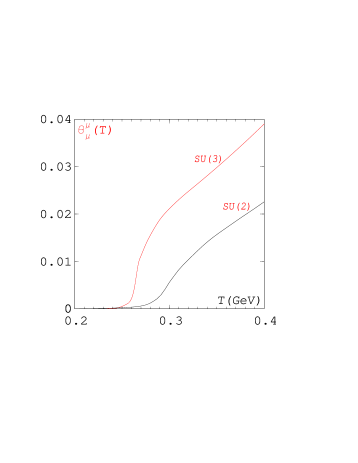
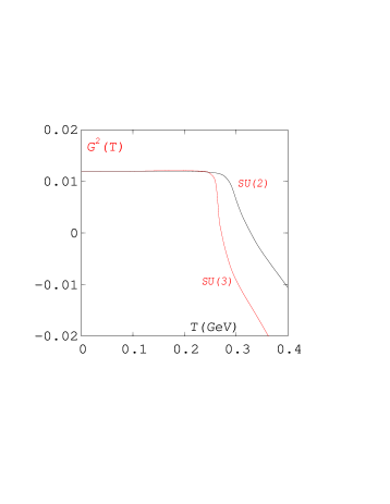
Figure 1: The left plots show ${\Theta}^{\mu}_{\mu}(T)$ for the lattice gauge theories $SU(2)$ and $SU(3)$ as indicated. The right plots show the corresponding gluon condensates. The values for the critical temperature $T_{\mbox{\scriptsize c}}=0.290,0.264$ GeV for $SU(2)$ and $SU(3)$, respectively. Both ordinates are in $GeV^{4}$.

In the left part of Figure 1 we compare the growth of $SU(2)$ and $SU(3)$ for the finite temperature part of the trace of the energy momentum tensor ${\Theta}^{\mu}_{\mu}(T)$. We note the continued growth of the trace with increasing temperature for the pure gauge theories. It was already contrasted [11] over a much larger temperature range the rapidity of growth in comparison where also properties of the critical behavior were included. The difference in the change of the thermal properties of the gluon condensate are then apparent with the assumed same vacuum structure, which is shown in the right part of Figure 1. These results of pure lattice gauge theory is completely consistent with the previous statement of Leutwyler [12] ”the gluon condensate does not disappear but becomes negative and large.” For the pure gauge theories there appears no reason for stopping the melting process as the temperature increases since gluons can be created without the limitations of a set scale other than that which comes out of the renormalization process at any given temperature.

4 The Chiral Condensate at Finite Temperature

In the presence of dynamical quarks another symmetry becomes important– the chiral symmetry. When the quarks have masses, this symmetry is automatically broken. The chiral symmetry is a property of the two different representations of $SL(2,\bf{C})$ denoted by $\bf{2}$ and $\bf{2^{*}}$ arising for the Dirac spinors. It is the presence of the quarks’ mass terms in the Dirac equation that formally breaks the chiral symmetry. This comes formally out of the nonconservation of the axial current $j^{\mu}_{5}$ as discussed above in equation (1.1) relating to the triangle diagrams, such that the chiral anomaly for QCD takes the form

$$\partial_{\mu}j^{\mu}_{5}\leavevmode\nobreak\ =\leavevmode\nobreak\ j_{5}\leavevmode\nobreak\ +{{k_{1}}\over{8\pi^{2}}}{{\bar{G}^{\mu\nu}_{a}}G^{a}_{\mu\nu}},$$ (4.1)

where $k_{1}$ is a constant. This situation has important implications in the case for finite temperatures where for $T$ sufficiently high the chiral symmetry is restored in the small mass limit. We shall discuss the implications of this both from the theoretical side and the numerical side where a finite small mass is present.  
We now look at the chiral condensate at finite temperatures using chiral perturbation theory. The low temperature expansion for two massless quarks can be written [12] in the following form:

$${{\langle\bar{\psi}_{q}{\psi}_{q}\rangle_{T}}\over{\langle\bar{\psi}_{q}{\psi}_{q}\rangle}_{0}}\leavevmode\nobreak\ =\leavevmode\nobreak\ 1\leavevmode\nobreak\ -\leavevmode\nobreak\ {1\over{8}}{T^{2}\over{F^{2}_{\pi}}}\leavevmode\nobreak\ -\leavevmode\nobreak\ {1\over{384}}{T^{4}\over{F^{4}_{\pi}}}\leavevmode\nobreak\ -\leavevmode\nobreak\ {1\over{288}}{T^{6}\over{F^{6}_{\pi}}}{\left\{ln{{\Lambda_{q}}\over{T}}\right\}}\leavevmode\nobreak\ +\leavevmode\nobreak\ O(T^{8})\leavevmode\nobreak\ +\leavevmode\nobreak\ O(\exp{-M\over{T}}),$$ (4.2)

where $F_{\pi}$ is the above mentioned pion decay constant and the scale $\Lambda_{q}$ is taken as approxamately $0.470GeV$. Leutwyler has shown at Quark Matter ’96 [12] that this expansion up to three loops remains very good at least to $0.100GeV$. Thus at low temperatures the probability of finding any given excited mass state is related to the exponentially small correction, which then has, indeed, a very little value. As the temperature grows the number of particle states begins to grow exponentially as would be indicated by the Hagedorn spectrum [19],which leads to a problem with this series at high temperatures. However, at low temperatures the excited states may be regarded as a dilute gas of free particles since the chiral symmetry supresses the interactions by a power of $T$ of this gas of excited states with the primary pionic component.  
Upon approaching the chiral symmetry restoration temperature $T_{\chi}$ the picture changes drastically. At this point the ratio $T/F_{\pi}$ is considerably greater than unity. It is here where one expects the chiral condensate to be very small or to have totally to have vanished. This effect has been studied recently numerically  [20] for two light flavors at finite temperature on the lattice. The results of this simulation is shown for ${{\langle\bar{\psi}_{q}{\psi}_{q}\rangle_{T}}/{\langle\bar{\psi}_{q}{\psi}_{q}\rangle}_{0}}$, which we simply write as $\langle\bar{\psi}{\psi}\rangle$. We show this quark condensate ratio as a function of the coupling $\beta$ for the range where the chiral symmetry is largely restored [20]. The left figure shows this ratio for two light quarks with a mass in lattice units of $0.02$ on a lattice of size $16^{3}\times 4$. The right figure shows different mass values from left to right of $0.02$, $0.0375$ and $0.075$ on $8^{3}\times 4$, $12^{3}\times 4$ and $16^{3}\times 4$ lattices. We should notice how the larger mass values slow the restoration down, which corresponds to moving the transition $T_{\chi}$ to higher temperatures or even eliminating it altogether as indicated by the flatness of the curves.  
The main quantities which were analyzed here were the various susceptibilities:  
1. The Polyakov loop susceptibility;

$${{\chi}_{L}}\leavevmode\nobreak\ =\leavevmode\nobreak\ N^{3}_{\sigma}{\left[\langle L^{2}\rangle\leavevmode\nobreak\ -\leavevmode\nobreak\ {\langle L\rangle}^{2}\right]},$$ (4.3)

2. The magnetic or chiral susceptibility;

$${{\chi}_{m}}\leavevmode\nobreak\ =\leavevmode\nobreak\ {T\over V}\leavevmode\nobreak\ {\sum\limits_{i=1}^{N_{f}}}{{\partial^{2}}\over{\partial m^{2}_{i}}}{\ln{\cal{Z}(T,V)}},$$ (4.4)

3. The thermal susceptibility;

$${{\chi}_{\theta}}\leavevmode\nobreak\ =\leavevmode\nobreak\ -{T\over V}\leavevmode\nobreak\ {\sum\limits_{i=1}^{N_{f}}}{{\partial^{2}}\over{\partial m_{i}\partial(1/T)}}{\ln{\cal{Z}(T,V)}}.$$ (4.5)

One compares the critical properties of ${{\chi}_{L}}$, ${{\chi}_{m}}$ and ${{\chi}_{\theta}}$ in order to establish the value of $T_{\chi}$ and its critical properties in the chiral limit where $m_{i}\rightarrow 0$. However, in numerical simulations $m_{i}$ must be taken to be finite– this means that one must use various different small values of $m_{i}$ on different sized lattices $N^{3}_{\sigma}\times N_{\tau}$. The procedure uses the lattice data to find the values around the peak of the susceptibility ${{\chi}_{m}}$ at $T_{\chi}$ for the smallest masses, with which one can determine the critical structure. A careful determination of the topological susceptibility relating to the chiral current correlations can be related to the square of the topological charge $Q^{2}_{T}$ [21] in the chiral limit, such that

$${N_{f}\over{m}}\langle Q^{2}_{T}\rangle\leavevmode\nobreak\ =\leavevmode\nobreak\ V{\langle\bar{\psi}{\psi}\rangle}_{m\rightarrow 0}.$$ (4.6)

Thus from the susceptibility one can arrive at the quark condensate $\langle\bar{\psi}{\psi}\rangle$. However, in this computation it is a major problem to properly set the temperature scale for small lattices with finite masses. The plots in Figure 2 are made with the coupling $\beta$ which may be compared with pure $SU(3)$ on one side and the two flavor dynamical quark simulations on the other [22]. In the case of pure $SU(3)$ the critical coupling $\beta_{c}$ for a ${16^{3}}\times 4$ lattice has the value [9] of about 5.70, which is considerably larger than the values of $\beta$ shown in Figure 2. However, for the two flavored dynamical quarks [22] the value of ${\beta}_{c}$ is around 5.40, which is still somewhat above the values shown in this figure.

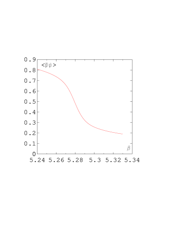
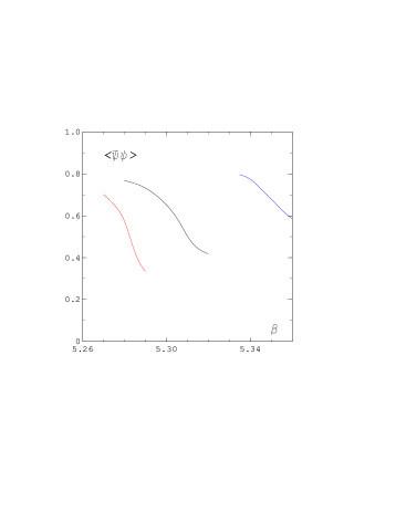
Figure 2: The left figure shows $<\bar{\psi}\psi>$ as a function of the coupling $\beta$ for the quark mass in lattice units $ma$= 0.02, which is normalized to the vacuum value of the chiral condensate. The right figure shows the same quantity with the different quark masses 0.02, 0.0375 and 0.075 from left to right [20].

In this section we have investigated the properties of the quark condensate $\langle\bar{\psi}{\psi}\rangle$ alone at various values of the coupling. However, here it is very difficult to immediately go over to a physical temperature scale in the same way as in the previous section for the pure gauge or gluon system. In what follows we shall look into the gluon condensate in the presence of dynamical quarks. Here we know that the presence of the quark masses are an immediate cause of scale symmetry breaking which of course change the scale of the system. This in turn changes the beta function as well as adds a term due to the mass renormalization. Thus the renormalization group equations are changed accordingly. This effect we shall discuss more thoroughly in the following section.

5 Gluon Condensate from the Trace Anomaly in the Presence of Quarks with finite Masses

The discovery of anomalous terms appearing as a finite value of the trace of the energy momentum tensor was pointed out as a result of nonperturbative evaluations in low-energy theorems [23] many years ago. Furthermore, it was also somewhat later realized how this factor arose with the process of renormalization in quantum field theory which became known as the trace anomaly [24] since it was found in relation to an anomalous trace of the energy momentum tensor.  
In the presence of massive quarks the trace of the energy-momentum tensor takes the following form [24] from the trace anomaly:

$$\langle\Theta^{\mu}_{\mu}\rangle\leavevmode\nobreak\ =\leavevmode\nobreak\ m_{q}\langle\bar{\psi}_{q}{\psi}_{q}\rangle\leavevmode\nobreak\ +\leavevmode\nobreak\ \langle G^{2}\rangle,$$ (5.1)

where $m_{q}$ is the light (renormalized) quark mass and ${\psi}_{q}$, $\bar{\psi}_{q}$ represent the quark and antiquark fields respectively. We include with these averages the renormalization group functions $\beta(g)$ and $\gamma(g,m)$, which appear in this trace from the renormalization process.  
Now we would like to discuss the changes in the computational procedure which arise from the presence of dynamical quarks with a finite mass. There have been recently a number of computations of the thermodynamical quantities in full QCD with two flavors of staggered quarks  [26, 27, 22], and with four flavors [28, 25]. These calculations are still not as accurate as those in pure gauge theory for several reasons. The first is the prohibitive cost of obtaining statistics similar to those obtained for pure QCD. So the error on the interaction measure is considerably larger. The second reason, perhaps more serious, lies in the effect of the quark masses currently simulated. They are still relatively heavy, which increases the contribution of the quark condensate term to the interaction measure. In fact, it is known that the vacuum expectation values for heavy quarks [13]is proportional to the vacuum gluon condensate or in the first approximation

$${\langle\bar{\psi}_{q}{\psi}_{q}\rangle}_{0}\leavevmode\nobreak\ =\leavevmode\nobreak\ {-1\over{12m_{q}}}{\langle G^{2}\rangle_{0}}.$$ (5.2)

Furthermore, there is an additional difficulty in setting properly the temperature scale even to the extent of rather large changes in the critical temperature have been reported in the literature depending upon the method of extraction. For two flavors of quarks the values of $T_{\mbox{\scriptsize c}}$ lie between $0.140GeV$ [22] and about $0.170GeV$  [29] which is considered presently a good estimate of the physical value for the critical temperature.  
We now indicate briefly how the thermodynamical information is obtained for the equation of state in terms of the lattice quantities. We start with the expectation values of the lattice action $\langle S\rangle$, which now contains some improved contributions for the pure guage actions  [25, 15] as well the contribution from the lattice fermions $\langle\bar{\chi}\chi\rangle$ as the chiral condensate as discussed in the last section. These quantities can be gotten from the partition function analogously to those in section 3. Explicitly it can be written as

$$\langle S\rangle\leavevmode\nobreak\ =\leavevmode\nobreak\ -{1\over{N^{3}_{\sigma}N_{\tau}}}\leavevmode\nobreak\ {{\partial}\over{\partial{\beta}}}{\ln{\cal{Z}}},$$ (5.3)

and

$$\langle{\bar{\chi}\chi}\rangle\leavevmode\nobreak\ =\leavevmode\nobreak\ -{1\over{N^{3}_{\sigma}N_{\tau}}}\leavevmode\nobreak\ {{\partial}\over{\partial{ma}}}{\ln{\cal{Z}}}.$$ (5.4)

For the computation of the finite temperature analogous to the pure gauge where the difference between $S_{0}$ and $S_{T}$ is used to compute the thermodynamics. Here we define

$${\overline{\langle S\rangle}}\leavevmode\nobreak\ =\leavevmode\nobreak\ {\langle S\rangle}_{0}\leavevmode\nobreak\ -\leavevmode\nobreak\ {\langle S\rangle}_{T}$$ (5.5)

and

$${\overline{\langle{\bar{\chi}\chi}\rangle}}\leavevmode\nobreak\ =\leavevmode\nobreak\ {\langle{\bar{\chi}\chi}\rangle}_{0}\leavevmode\nobreak\ -\leavevmode\nobreak\ {\langle{\bar{\chi}\chi}\rangle}_{T}.$$ (5.6)

Now we define instead of the lattice beta function two similar quantities called [25] $R_{\beta}$ and $R_{m}$. We write

$$R_{\beta}\leavevmode\nobreak\ ={d\leavevmode\nobreak\ {\beta}\over{d\leavevmode\nobreak\ {\ln}a}},$$ (5.7)

and

$$R_{m}\leavevmode\nobreak\ ={d\leavevmode\nobreak\ {ma}\over{d\leavevmode\nobreak\ {\ln}a}}.$$ (5.8)

We are now able to define a new interaction measure in the presence of dynamical quarks $\Delta_{m}(T)$ in terms of these quantities, so that

$$\Delta_{m}(T)\leavevmode\nobreak\ =\leavevmode\nobreak\ -{N^{4}_{\tau}}\leavevmode\nobreak\ {\left[R_{\beta}{\overline{\langle S\rangle}}\leavevmode\nobreak\ -\leavevmode\nobreak\ R_{m}{\overline{\langle{\bar{\chi}\chi}\rangle}}\right]}.$$ (5.9)

Here we note the explicit effect of the quark condensate in the computation of $\Delta_{m}(T)$.  
Here it is appropriate to briefly explain another approach [25] to the setting of the temperature scale for the lattice computations. An effective coupling can be defined ${\beta}_{eff}$ in terms of the gluonic part of the action as

$${\beta}_{eff}\leavevmode\nobreak\ ={12\over{{\langle S\rangle}(\beta)}}.$$ (5.10)

Then the dependence is used to calculate the derivative $R_{\beta}$ with the help of the asymptotic two loop renormalization group equation. This procedure [25] also fixes the temperature scale so that

$${T\over T_{c}}\leavevmode\nobreak\ =\leavevmode\nobreak\ {\left({\beta}_{eff}\over{\beta_{c}}\right)}^{-77/625}\exp{\left({{4\pi^{2}}\over 25}(\beta_{eff}-\beta_{c})\right)}.$$ (5.11)

This method allows us to establish the temperature in comparison to the critical temperature.  
We are now able to write down an equation for the temperature dependence of the thermally averaged trace of the energy momentum tensor including the effects of the light quarks from $\Delta_{m}(T)$ so that

$$\langle\Theta^{\mu}_{\mu}\rangle_{T}\leavevmode\nobreak\ =\leavevmode\nobreak\ \Delta_{m}(T)\times T^{4}.$$ (5.12)

The thermally averaged gluon condensate is computed including the light quarks in the trace anomaly using the equation (5.1) and the interaction measure in $\langle\Theta^{\mu}_{\mu}\rangle_{T}$ to get

$$\langle G^{2}\rangle_{T}\leavevmode\nobreak\ =\leavevmode\nobreak\ \langle G^{2}\rangle_{0}\leavevmode\nobreak\ +\leavevmode\nobreak\ m_{q}\langle\bar{\psi}_{q}{\psi}_{q}\rangle_{0}\leavevmode\nobreak\ \leavevmode\nobreak\ -\leavevmode\nobreak\ m_{q}\langle\bar{\psi}_{q}{\psi}_{q}\rangle_{T}\leavevmode\nobreak\ \leavevmode\nobreak\ -\leavevmode\nobreak\ \langle\Theta^{\mu}_{\mu}\rangle_{T}.$$ (5.13)

It is possible to see from this equation that at very low temperatures the additional contribution to the temperature dependence of the gluon condensate from the quark condensate is rather insignificant and disappears at zero temperature. However, in the range where the chiral symmetry is being restored there is an additional effect from the term $\langle\bar{\psi}_{q}{\psi}_{q}\rangle_{T}$, which lowers $\langle G^{2}\rangle_{T}$. Well above $T_{\mbox{\scriptsize c}}$ after the chiral symmetry has been mostly restored the only remaining effect of the quark condensate is that of $m_{q}\langle\bar{\psi}_{q}{\psi}_{q}\rangle_{0}$. It is known [13] that this term then the gluon condensate of the vacuum. Thus we expect [11] that for the light quarks the temperature dependence can only be important below $T_{\mbox{\scriptsize c}}$. In the case of the chiral limit $m_{q}\rightarrow 0$ the equation (5.13) takes the form of Leutwyler’s equation  (2.3) as, of course, it should because Leutwyler used two massless quarks [12]. For the smaller values of the simulated quark masses in lattice units of 0.01 to 0.02 $\langle\bar{\psi}_{q}{\psi}_{q}\rangle_{T}$ has mostly disappeared in the range where $\langle G^{2}\rangle_{T}$ differs from $\langle G^{2}\rangle_{0}$.  
In order to see this effect, we look at Figure 3 where the data of various simulations of finite temperature QCD with dynamical quarks is used to show $\langle G^{2}\rangle_{T}$ as a function of T. Included in this figure is a plot of the pure gauge $SU(3)$ with its $T_{\mbox{\scriptsize c}}$ rescaled to $0.150\leavevmode\nobreak\ GeV$, which is shown with the broken lines [11]. The Bielefeld four flavor data [28, 25] is used to compute $\langle G^{2}\rangle_{T}$ [11] shown in the open squares. The masses in these simulations are rather large, 0.05 and 0.1 in lattice units. These quite large masses do cause the quark terms to be more important at a considerably lower temperature. Also since there are four massive flavors, the total contribution is larger. Thus at lower temperatures below $T_{\mbox{\scriptsize c}}$ the points for $\langle G^{2}\rangle_{T}$ lie considerably below those values for the pure gauge theory. Starting at around $0.100\leavevmode\nobreak\ GeV$ we can see [11] a difference from $\langle G^{2}\rangle_{0}$. However, at high temperatures we notice that the points are well above the pure gauge theory.  
For the two flavor quarks we show two sets of published data from the MILC collaboration [26, 27, 22], both of which involved a rather extensive analysis of various thermodynamical quantities. The masses in these cases are somewhat lighter, 0.0125 and 0.025 in lattice units. The earlier data [26, 27],which has been used [11] to compute $\langle G^{2}\rangle_{T}$, is indicated by the solid squares in Figure 3. Its behavior shows a smaller decrease than the four flavor data and, indeed, follows more closely the pure $SU(3)$ data [9] at lower temperatures. At or slightly above $T_{\mbox{\scriptsize c}}$ it appears that the data points for $\langle G^{2}\rangle_{T}$ even rise [11]. This apparent effect does not seem to be very physically reasonnable or, at best, it is unexpected! We would physically expect the raising of the system to higher temperatures to continually reduce the amount of gluon condensate. However, the newer data [22], which is indicated by the crosses in Figure 3, follows closely the earlier below $T_{\mbox{\scriptsize c}}$, but falls considerably below the solid squares above the critical temperature. Nevertheless, the data points at the higher temperatures still do not decrease in value very rapidly so that within the errorbars the decondensation appears to remain flat. This tendency is clearly very different from the pure gauge theory as shown in Section 3.

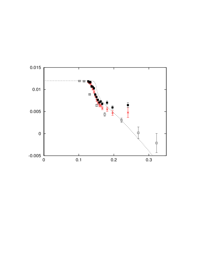
Figure 3: The gluon condensate $<G^{2}>_{T}$ in $GeV^{4}$ with dynamical quarks is plotted against the temperature T in $GeV$ in the following cases: pure gauge theory [9] (broken lines); Bielefeld computation [25] (open squares); MILC’96 [27] (filled squares); MILC’97 [22] (crosses)

As an end to this discussion of the gluon condensate in QCD we will mention a few other points. Where in simulations on pure $SU(N_{c})$ gauge theory we could depend on considerable precision in the determination of $T_{\mbox{\scriptsize c}}$ and $\Delta(T)$ as well as numerous other thermodynamical functions, it is still not the case for the theory with dynamical quarks. The statistics for the numerical measurements are generally smaller. The determination of the temperature scale is thereby hindered so that it is harder to clearly specify a given quantity in terms of $T$. Thus, in general, we may state that the accuracy for the full QCD is way down when compared to the computations of the pure lattice gauge theories. However, there is a point that arises from the effect that the temperatures in full QCD are generally lower, so that $\Delta(T)\times T^{4}$ is much smaller [11]. Here we can only speculate with the present computations [26, 27, 28, 22]. Nevertheless, there could be an indication of how the stability of the full QCD keeps $\langle G^{2}\rangle_{T}$ positive for $T\leavevmode\nobreak\ >\leavevmode\nobreak\ T_{\mbox{\scriptsize c}}$. The condensates in full QCD have also been considered by Koch and Brown [30]. However, the lattice data which they used were not obtained using a non-perturbative method, nor was the temperature scale obtained from the full non-perturbative beta-function. Finally we should remark that the determination of the gluon condensate for the vacuum is more significant in the presence of dynamical quarks. At the present stage of the computations the newer MILC results[22] would prefer the earlier value of $0.012\leavevmode\nobreak\ GeV^{4}$ [13] in contrast to the newer value of $0.0226\leavevmode\nobreak\ GeV^{4}$ [14] only in the sense that the former favors a larger proportion of the condensate to have vanished near the critical temperature.

6 Anomalous Currents at Finite Temperature

In the previous sections we noticed that the fact that the trace of the energy momentum tensor does not vanish for the strong interactions has important implications for the equation of state. Here we shall discuss some more theoretical results relating to $\Theta^{\mu}_{\mu}(T)$ or more exactly its relation to the corresponding differential four-forms on a four-manifold coming from $G^{2}d^{4}x$, the gluon condensate in four dimensional space-time, where $d^{4}x$ is short for the wedge product of the four different space-time differentials. This situation brings about certain properties with respect to the dilatation current as well as the special conformal currents, both of which are not conserved. On the other hand we have the anomalous chiral current which relates to the other four-form arising from  ${\bar{G}}Gd^{4}x$ resulting from the nonconservation of the chiral current. In absolute magnitude this current has less importance at high temperatures for disappearing quark masses since the chiral symmetry is then completely restored . Nevertheless, it obviously plays a role near the deconfinement temperature of a system with finite quark masses through the above noted changes in the gluon condensate at finite temperature.  
The dilatation current $D^{\mu}$ has been defined above in terms of the position four-vector $x^{\mu}$ and the energy momentum tensor  $T^{\mu\nu}$ as simply the product $x_{\alpha}T^{\mu\alpha}$ as moments of the energy density. In the case of general energy momentum conservation one can find [31] quite simply a relation to the equation of state. We now look into a volume in four dimensional space-time ${\cal V}_{4}$ containing all the quarks and gluons at a fixed temperature $T$ in equilibrium. The flow equation (1.2) holds when the energy momentum and all the (color) currents are conserved over the surface $\partial{\cal V}_{4}$ of the properly oriented four-volume ${\cal V}_{4}$, which yields

$$\oint_{\partial{\cal V}_{4}}{\cal D}_{\mu}dS^{\mu}\leavevmode\nobreak\ =\leavevmode\nobreak\ \int_{{\cal V}_{4}}T^{\mu}_{\mu}dV_{4},$$ (6.1)

We have already introduced [10] the dyxle three-form as  ${\cal D}_{\mu}dS^{\mu}$ on the three dimensional surface $\partial{\cal V}_{4}$. The dyxle is the dual form to  $D_{\mu}dx^{\mu}$ the dilatation current one-form [32] in four dimensional space-time. It represents the flux through this closed surface acting as the boundry of the volume ${\cal V}_{4}$. On the right hand side of (6.1) the integrated form  $\int_{{\cal V}_{4}}T^{\mu}_{\mu}dV_{4}$ is an action or flux integral involving the equation of state. Since $T^{\mu}_{\mu}>0$, the action integral is not zero. This action integral gets quantized with the fields through the renormalization process. It acts as the source term.  
An analogous form can be defined for the four special conformal currents which we shall call the fourspan. The dual forms are derived from the equation (1.3) in a similar manner to the dyxle, which yields

$$\oint_{\partial{\cal V}_{4}}{\cal K}^{\alpha}_{\mu}dS^{\mu}\leavevmode\nobreak\ =\leavevmode\nobreak\ \int_{{\cal V}_{4}}{2{x^{\alpha}}}T^{\mu}_{\mu}dV_{4},$$ (6.2)

Of most immediate interest to us here is really the finite temperature part of the dyxle ${\cal{D}}(T)_{\mu}{dS^{\mu}}$ in relation to the quark-gluon condensates in QCD. This physical quantity represents the flux as force through an area at a temperature $T$. Directly interpreted the dyxle is the first moment in space-time of the energy-momentum. The vacuum part just represents a fixed quantization where its value comes out of the renormalization of the loops from the QCD beta and gamma functions. When we set only ${\Theta}^{\mu}_{\mu}(T)$ into the dyxle equation (6.1), we get the integral over a bounded region of space-time in terms of the actual four-forms in vacuo and at finite temperature $\leavevmode\nobreak\ \int_{{\cal V}_{4}}{\left(G^{2}_{0}\leavevmode\nobreak\ -\leavevmode\nobreak\ G^{2}(T)\right)}dV_{4}$, which comes directly out of Leutwyler’s equation (2.3). This integral is clearly related to the interaction measure $\Delta(T)$ in a bounded region of space-time. Hereby the problem is reduced to one in homology relating to the topology of the space-time. Unfortunately, The topological properties of the fourspan at finite temperature is not so directly related with the lattice results. The four conformal currents are each related to higher moments of the energy-momentum in space-time. Therefore, each of the four currents have a different moment structure relating to a different second moments of the energy-momentum. Here we are able at this time to say very little numerically about them.  
The flux integrals arising in finite temperature QCD remind us of some geometrically much simpler properties of the electromagnetic flux, which is usually described in terms of Gauss’ Law using a closed two dimensional surface through which the electromagnetic fields penetrate. The nature of this two dimensional spatial surface is easily represented as a subspace of a three dimensional Euclidean geometry. Our envisioning now becomes a bit more difficult with a three dimensional surface for a four dimensional space- time where we try to attibute this flux structure to a dual three-form with the property that the dyxle has a ”source term” arising from the equation of state in four dimensional space-time. This is the statement of the integral form of the above equation (6.1). It would be nice if we were able to directly relate this statement to that of confinement or deconfinement. However, as a phase transition it is presently unclear how to relate these results to a single simple order parameter in all cases.

7 Summary, Conclusions and Speculations

The main investigation of this paper involves the study of nonconserved anomalous currents using numerical results relating to the existence of particular four-forms in finite temperature QCD. For the pure gauge theory we consider only the trace anomaly and its implications on the gluon condensate as discussed in the third section. The presence of quarks with finite masses brings about an interplay between the renormalization causing scale breaking and the explicit scale breaking due to the masses. Here both anomalies must be considered.  
Although the explicit nature of the two anomalies have quite different physical origins, the general effect on the gluon condensate at high temperature is quite similar. The trace anomaly alone reflecting the breaking of the scale and conformal symmetries, while the chiral anomaly comes from the two different representations of $SL(2,\bf{C})$ representing the two chiralities. In the case of the scale and conformal symmetries there is never restoration, but only a change in the breaking due to the temperature dependence. For the chiral symmetry it is resored at high temperatures up to the effects of the quark masses. For the larger quark masses the breaking at high temperature remains considerable as we saw in the fourth section. In the fifth section we looked at the combined effects of the two anomalies but only for fairly small quark masses, that is well under the energy scale of the critical temperature. Thus the explicit mass effect with the gluon condensate arising with the quark condensate is very small, which lets us use the numbers directly from the simulations. At the moment we can only at most speculate about the role of the heavier quarks with a mass around the energy value of $T_{\mbox{\scriptsize c}}$. Here a brief thought on it may be of value.  
The speculations are on a three quark model with two light quarks of less than 10 MeV and one heavy quark of about 150 MeV representing u-, d- and s-quarks respectively. The energy scale of the s-quark’s mass is very close to that of $T_{\mbox{\scriptsize c}}$. Thus any sizable s-quark condensate would have a sizable contribution to the gluon condensate at finite temperature through equation (5.13). The very heavy quark condensates are given by (5.2), which gives an amount inversely proportional to the quark mass. Thus one would expect the charmed as well as, of course, the bottom and top quarks to have a very small role at $T_{\mbox{\scriptsize c}}$ in the decondensation of the gluons. The very heavy quarks are those which provide the static gluon fields without the dynamical effects.

8 Acknowledgements

The author would like to thank Rolf Baier and Krzysztof Redlich for many very helpful discussions. Also a special thanks goes to Graham Boyd with whom many of the computations were carried out. He is grateful to the Bielefeld group for providing their data, and especially to Jürgen Engels for the use of his programs and many valuable explanations of the lattice results. He would like to recognize the support of ZiF for Summer 1998 in the project ”Multiscale Phenomena and their Simulation on Massively Parallel Computers” led by Frithjof Karsch and Helmut Satz. He would also like to thank Edwin Laermann for discussions and the use of the Bielefeld data for the chiral condensate and Andreas Peikert for information on the two flavor critical temperature. Many thanks go to Carleton DeTar for sending personally the newer data from the MILC collaboration. Finally a word of thanks goes to Toni Rebhan and all the organizers of the ”Workshop on Quantization, Generalized BRS Cohomology and Anomalies” at the Erwin Schrödinger Institute in Vienna, Austria.

References

- [1] A. Einstein, Annalen der Physik (Vierte Folge), Band , 891; Band , 639 (1905); Band , 627 (1906).
- [2] H. Bateman, Proceedings London Mathematical Society (second series) , 228 (1909).
- [3] E. Bessel-Hagen, Mathematische Annalen, , 258 (1921).
- [4] E. Noether, Göttinger Nachtrichten, 235 (1918).
- [5] S. L. Adler, Physical Review , 2426 (1969); J. S. Bell and R. Jackiw, Nuovo Cimento , 47 (1969).
- [6] R. A. Bertlmann, , Clarendon Press, Oxford, 1996; T. Kugo, , Springer, Berlin, 1997; German translation by S. Heusler from the original Japanese edition, 1989.
- [7] S.B.Treiman, R.Jackiw, B.Zumino and E.Witten (Editors), , Princeton University Press, Princeton, N. J., 1985.
- [8] J. Engels, F. Karsch and K. Redlich, Nuclear Physics, , 295 (1995).
- [9] G. Boyd, J. Engels, F. Karsch, E. Laermann, C. Legeland, M. Lütgemeier and B. Petersson, Physical Review Letters , 4169 (1995); Nuclear Physics , 419 (1996).
- [10] D. E. Miller, Acta Physica Polonica, , 2937 (1997).
- [11] G. Boyd and D. E. Miller, “The Temperature Dependence of the Gluon Condensate from Lattice Gauge Theory”, Bielefeld Preprint, BI-TP 96/28, August 1996, hep-ph/9608482.
- [12] H. Leutwyler, “Deconfinement and Chiral Symmetry” in , Vol. 2, P. M. Zerwas and H. A. Kastrup (Eds.), World Scientific, Singapore, 1993, pp. 693-716; further details of this discussion were presented in an plenary lecture at QUARK MATTER ’96, Heidelberg, 24. May 1996.
- [13] M. A. Shifman, A. I Vainshtein and V. I. Zakharov, Nuclear Physics , 385,448,519 (1979).
- [14] S. Narison, Physics Letters , 121 (1995); , 162 (1996).
- [15] J. Engels, F. Karsch and T. Scheideler, ”Determination of Anisotropy Coefficients for SU(3) Gauge Actions from the Integral and Matching Methods”, Bielefeld Preprint, BI-TP 99/02, April 1999. This newer work goes into a careful discussion of the accuracy of known methods and their equivalence in lattice guage theory.
- [16] L. D. Landau and E. M. Lifshitz, , Volume 2, “Classical Theory of Fields”, Pergamon Press, Oxford, England, Chapter IV; Volume 6, “Fluid Mechanics”, Pergamon Press, Oxford, England, Chapter XV, pp. 505-514.
- [17] T. Muta, , World Scientific, Singapore, Second Edition 1998.
- [18] J. Engels, F. Karsch, H. Satz and I. Montvay, Nuclear Physics , 545 (1982); J. Engels, J. Fingberg, K. Redlich, H. Satz and M. Weber, Zeitschrift für Physik , 341 (1989); J. Engels, J. Fingberg, F. Karsch, D. Miller and M. Weber, Physics Letters , 625 (1990).
- [19] R. Hagedorn, Supplemento al Nuovo Cimento, Volume III, 147 (1965).
- [20] E. Laermann, Proceedings of the International Workshop on Lattice QCD on Parallel Computers, Nuclear Physics B (Proceedings Supplement), , 180 (1998).
- [21] F. C. Hansen and H Leutwyler, Nuclear Physics , 201 (1991).
- [22] C. Bernard, T. Blum, C. DeTar, S. Gottlieb, K. Rummukainen, U. M. Heller, J. E. Hetrick, D. Toussaint, L. Kärkkäinen, R. L. Sugar and M. Wingate, Physical Review , 6861 (1997); We use explicitly the numerical data associated with Figure 7 on page 6865 in our Figure 3.
- [23] R. J. Crewther, Physical Review Letters, , 1421 (1972); M. S. Chanowitz and J. Ellis, Physics Letters, , 397 (1972); M. S. Chanowitz and J. Ellis, Physical Review, , 2490 (1973).
- [24] S. L. Adler, J. C. Collins and A. Duncan, Physical Review , 1712 (1977). J. C. Collins, A. Duncan and S. D. Joglekar, Physical Review , 438 (1977); N. K. Nielsen, Nuclear Physics , 212 (1977).
- [25] J.Engels, R. Joswig, F. Karsch, E. Laermann, M. Lütgemeier, and B. Petersson, Physics Letters , 210 (1997).
- [26] T. Blum, L. Kärkkäinen, D. Toussaint and S. Gottlieb, Physical Review , 5153 (1995).
- [27] C. Bernard et al., Proceedings of Lattice’96, Nuclear Physics B(Proceedings Supplement) , 442 (1997).
- [28] E. Laermann, Proceedings of Quarkmatter’96, Nuclear Physics , 1c (1996); F. Karsch et al., Proceedings of Lattice’96, Nuclear Physics B(Proceedings Supplement), , 413 (1997).
- [29] E. Laermann, Proceedings of the XVth International Symposium on Lattice Field Theory, Nuclear Physics B (Proceedings Supplement), , 114 (1998).
- [30] V. Koch and G. E. Brown, Nuclear Physics (1993) 345.
- [31] R. Jackiw, “Topological Investigations of Quantized Gauge Theories”, in , S. B. Treiman et al. (Eds.), cited above, pp. 211-359.
- [32] H. Flanders, , Second Edition, Dover, New York, 1989; see especially sections 4.6, 5.9 and 10.6.