DTP/99/88

hep-ph/9907523

Application of the negative-dimension approach to massless scalar box integrals

C. Anastasiou, E. W. N. Glover and C. Oleari Department of Physics, University of Durham, Durham DH1 3LE, England

We study massless one-loop box integrals by treating the number of space-time dimensions $D$ as a negative integer. We consider integrals with up to three kinematic scales ($s$, $t$ and either zero or one off-shell legs) and with arbitrary powers of propagators. For box integrals with $q$ kinematic scales (where $q=2$ or 3) we immediately obtain a representation of the graph in terms of a finite sum of generalised hypergeometric functions with $q-1$ variables, valid for general $D$. Because the power each propagator is raised to is treated as a parameter, these general expressions are useful in evaluating certain types of two-loop box integrals which are one-loop insertions to one-loop box graphs. We present general expressions for this particular class of two-loop graphs with one off-shell leg, and give explicit representations in terms of polylogarithms in the on-shell case.

1 Introduction

Box integrals play an important role in the perturbative description of $2\,\mbox{$\rightarrow$}\,2$ scattering processes. Classic examples at one-loop include the scattering of light-by-light [1] and the scattering of partons [2]. Recent improvements of experimental measurements demand even more precise theoretical predictions and there is significant interest in determining $2\,\mbox{$\rightarrow$}\,2$ cross sections at the two-loop order. To achieve this goal requires the evaluation of certain master two-loop graphs, such as the planar double-box graph [3, 4], or some one-loop box integrals with bubble insertions on one of the propagators.

In 1987, Halliday and Ricotta [5] suggested a method of calculating loop integrals based on treating the number of space-time dimensions $D$ as a negative integer. Because loop integrals are analytic in $D$ (and also in the powers of the propagators), this is a valid procedure and, although the intermediate steps may be carried out in negative $D$ (and in particular series expansions can be made), $D$ remains a parameter of the calculation and can be taken to be positive after integration. The problem of loop integration is replaced by that of handling infinite series. This idea was neglected for some time until Suzuki and Schmidt started a more systematic application of the negative dimension method (NDIM) to a number of two-loop integrals [6], three-loop integrals [7], one-loop tensor integrals [8] as well as the one-loop massive box integral for the scattering of light by light [9]. In this last paper, Suzuki and Schmidt discovered that as well as reproducing the known hypergeometric-series representations of Ref. [10], valid in particular kinematic regions, hypergeometric solutions valid in other kinematic domains are simultaneously obtained. Of course, all of these solutions are related by analytic continuation. However, it is easy to envisage integrals that yield hypergeometric functions where the analytic continuation formulae are not known a priori. In these cases, having series expansions directly available in all kinematic regions may be very useful.

Recently, we have generalised this method to describe massive $n$-point one-loop graphs with general powers of the propagators and arbitrary dimension $D$ [11]. For graphs with $m$ mass scales, $q$ external momentum scales and $n$ legs, we have written down a template series solution with $(m+q+n)$ summation indices, together with a linear system of $(n+1)$ constraints. The template solution is completely general, while the constraints can be read off the specific Feynman graph. By solving the system of constraints, we obtain many solutions with $(m+q-1)$ summation indices, each of which can be identified directly as a hypergeometric function in the appropriate convergence region. The full solution in a particular kinematic region is formed by adding the solutions that converge in that region. It turns out that by keeping the parameters general, it is easier to identify the regions of convergence of the hypergeometric series and, therefore, which hypergeometric functions to group together. This has the additional advantage of allowing a connection with the general tensor-reduction program based on integration by parts of Refs. [12, 13] where the tensor integrals are linear combinations of scalar integrals with either higher dimension or propagators raised to higher powers. It is the goal of this paper to consider massless box integrals and to obtain expressions in terms of hypergeometric functions valid for general powers of the propagators and arbitrary dimension.

Our paper is arranged as follows. In Sec. 2 we show how NDIM can be applied to construct the template solutions for one-loop box integrals together with the linear system of constraints that relates the powers of the propagators in the loop integral to the summation variables. We give the expressions for the solutions in different kinematic regions for massless scalar box integrals with one off-shell leg and for the on-shell case in terms of hypergeometric functions of one or two variables. In both cases, $D$ is arbitrary and the propagators are raised to arbitrary powers. As an application of the general formulae, in Sec. 3 we consider a particular class of two-loop box integrals which are one-loop box graphs with bubble insertions on one of the legs. We give general formulae for the scalar integrals with three powers of propagators set to unity and one propagator (corresponding to the place where the one-loop insertion is made) kept arbitrary. In this case, identities amongst hypergeometric functions can be used to simplify the general expressions. We show how to evaluate the hypergeometric functions in the on-shell case and, by making a series expansion in $\epsilon=(4-D)/2$, give explicit expressions in terms of logarithms and polylogarithms for the relevant two-loop scalar integrals. Finally, our findings are summarised in Sec. 4.

2 The general massless one-loop box integral

The generic massless one-loop box integral in $D$-dimensional Minkowski space with loop momentum $k$ is given by

$$I^{D}_{4}\left(\nu_{1},\nu_{2},\nu_{3},\nu_{4};\{Q_{i}^{2}\}\right)=\int\frac{d^{D}k}{i\pi^{D/2}}\frac{1}{A_{1}^{\nu_{1}}\ldots A_{4}^{\nu_{4}}},$$ (2.1)

where, as indicated in Fig. 1, the external momenta $k_{i}$ are all incoming so that $\sum_{i=1}^{4}k_{i}^{\mu}=0$ and the massless propagators have the form

$$A_{1} = k^{2}+i0,$$

$$A_{i} = \left(k+\sum_{j=1}^{i-1}k_{j}\right)^{2}+i0\qquad{i\neq 1}.$$ (2.2)

The external momentum scales are indicated with $\{Q_{i}^{2}\}$. In our case they are the Mandelstam variables $s=\left(k_{1}+k_{2}\right)^{2}$, $t=\left(k_{2}+k_{3}\right)^{2}$ and the external masses $k_{i}^{2}=M_{i}^{2}$. In this paper we will focus on box integrals with at most one off-shell leg, so that we have $k_{i}^{2}=0$ for $i=1,2,3$, and $k_{4}^{2}=M^{2}$. For standard integrals, the powers $\nu_{i}$ to which each propagator is raised are usually unity. However, we wish to leave the powers as general as possible. Later on we will use these general expressions to derive some results for two-loop box integrals with one-loop insertions on the propagators.

Figure 1: The one-loop box diagram.

We can rewrite Eq. (2.1) using Schwinger parameters $x_{i}$, so that

$$I^{D}_{4}\left(\nu_{1},\nu_{2},\nu_{3},\nu_{4};\{Q_{i}^{2}\}\right)=\int{\cal D}x\int\frac{d^{D}k}{i\pi^{D/2}}~{}\exp\left(\sum_{i=1}^{4}x_{i}A_{i}\right),$$ (2.3)

where we have used the shorthand

$$\int{\cal D}x=(-1)^{\sigma}\left(\prod_{i=1}^{4}\frac{1}{\Gamma(\nu_{i})}\int^{\infty}_{0}dx_{i}x_{i}^{\nu_{i}-1}\right),$$ (2.4)

with

$$\sigma=\sum_{i=1}^{4}\nu_{i}.$$ (2.5)

Performing the Gaussian integral in a straightforward way we have the usual Minkowski-space result for massless integrals

$$I^{D}_{4}\left(\nu_{1},\nu_{2},\nu_{3},\nu_{4};\{Q_{i}^{2}\}\right)=\int{\cal D}x\frac{1}{{\cal P}^{D/2}}~{}\exp({\cal Q}/{\cal P}),$$ (2.6)

where

$${\cal P}=x_{1}+x_{2}+x_{3}+x_{4},$$ (2.7)

while for box integrals with one off-shell leg ($k_{4}^{2}=M^{2}$)

$${\cal Q}=x_{1}x_{3}\,s+x_{2}x_{4}\,t+x_{1}x_{4}\,M^{2}.$$ (2.8)

As usual, in the physical region $t<0$ and $s>0$.

To evaluate the integral further, we adopt the suggestion of Halliday and Ricotta [5] and treat the number of dimensions $D$ as a negative integer. This is valid because the loop integral is an analytic function of $D$. We follow the approach suggested by Suzuki and Schmidt [6]–[9] and detailed in [11] by viewing Eqs. (2.3) and (2.6) as existing in negative dimensions. We make a series expansion in $x_{i}$ in both Eqs. (2.3) and (2.6). The role of having $D<0$ is that the power of ${\cal P}$ is now positive allowing a multinomial expansion. Following the notation of [11], we have

$$I_{4}^{D}(\nu_{1},\nu_{2},\nu_{3},\nu_{4};s,t,M^{2})$$ (2.9)

$$= \int{\cal D}x\sum_{n_{1},\ldots,n_{4}=0}^{\infty}\int\frac{d^{D}k}{i\pi^{D/2}}\frac{(x_{1}A_{1})^{n_{1}}}{n_{1}!}\frac{(x_{2}A_{2})^{n_{2}}}{n_{2}!}\frac{(x_{3}A_{3})^{n_{3}}}{n_{3}!}\frac{(x_{4}A_{4})^{n_{4}}}{n_{4}!}$$

$$= \int{\cal D}x\sum_{{p_{1},\ldots,p_{4}=0\atop{q_{1},\ldots,q_{3}=0}}}^{\infty}\frac{\left(x_{1}x_{3}s\right)^{q_{1}}\left(x_{2}x_{4}t\right)^{q_{2}}\left(x_{1}x_{4}M^{2}\right)^{q_{3}}}{q_{1}!q_{2}!q_{3}!}\frac{x_{1}^{p_{1}}\ldots x_{4}^{p_{4}}}{p_{1}!\ldots p_{4}!}\,(p_{1}+p_{2}+p_{3}+p_{4})!,\phantom{aaa}$$

with the constraint

$$q_{1}+q_{2}+q_{3}+p_{1}+p_{2}+p_{3}+p_{4}=-\frac{D}{2},$$ (2.10)

that ensures that the power of ${\cal Q}$ and ${\cal P}$ match up correctly. The integers $p_{i}$ and $q_{i}$ are introduced in making the multinomial expansions of ${\cal P}$ and ${\cal Q}$ respectively. If more than one leg is off shell, then there will be additional terms in ${\cal Q}$ leading to more summation variables. Similarly, if we take the $M^{2}\,\mbox{$\rightarrow$}\,0$ limit, this is the same as fixing $q_{3}=0$ in Eq. (2.9).

The $x_{i}$ are independent variables so that for the equality (2.9) to hold, the integrands themselves must be equal. Therefore, by selecting the coefficient of the powers of $x_{i}^{-\nu_{i}}$, where $\nu_{i}=-n_{i}$, on both sides of the equality we find

$$I_{4}^{D}(\nu_{1},\nu_{2},\nu_{3},\nu_{4};s,t,M^{2})$$ (2.11)

$$= \sum_{{p_{1},\ldots,p_{4}=0\atop{q_{1},\ldots,q_{3}=0}}}^{\infty}\frac{\Gamma\left({1+p_{1}+p_{2}+p_{3}+p_{4}}\right)}{\Gamma\left({1+q_{1}}\right)\Gamma\left({1+q_{2}}\right)\Gamma\left({1+q_{3}}\right)}\left(\prod_{i=1}^{4}\frac{\Gamma\left({1-\nu_{i}}\right)}{\Gamma\left({1+p_{i}}\right)}\right)\,s^{q_{1}}t^{q_{2}}\left(M^{2}\right)^{q_{3}},$$

subject to the system of constraints

$$q_{1}+q_{3}+p_{1} = -\nu_{1},$$

$$q_{2}+p_{2} = -\nu_{2},$$

$$q_{1}+p_{3} = -\nu_{3},$$ (2.12)

$$q_{2}+q_{3}+p_{4} = -\nu_{4},$$

$$q_{1}+q_{2}+q_{3}+p_{1}+p_{2}+p_{3}+p_{4} = -D/2.$$

There are seven summation variables and five constraints so that two variables will be unconstrained. The procedure for developing the solution for the loop integral further is detailed in Ref. [11]. Each of the fifteen solutions of the system is inserted into the template solution (2.11). For example, solving with respect to the indices $\{q_{1},q_{2}\}$, we find

$$p_{1} = \nu_{2}+\nu_{3}+\nu_{4}+q_{2}-D/2,$$

$$p_{2} = -\nu_{2}-q_{2},$$

$$p_{3} = -\nu_{3}-q_{1},$$

$$p_{4} = \nu_{1}+\nu_{2}+\nu_{3}+q_{1}-D/2,$$

$$q_{3} = -q_{1}-q_{2}+D/2-\nu_{1}-\nu_{2}-\nu_{3}-\nu_{4},$$

which is then applied to (2.11). $\Gamma$ functions that depend on the unconstrained variables $q_{1}$ and $q_{2}$ are converted into Pochhammer symbols

$$(z,n)\equiv\frac{\Gamma(z+n)}{\Gamma(z)},$$ (2.13)

because they are the most suitable way to write generalized hypergeometric functions. Denoting this solution as $I^{\{q_{1},q_{2}\}}$ and introducing the shorthand notation

$$\nu_{ij}=\nu_{i}+\nu_{j},\qquad\nu_{ijk}=\nu_{i}+\nu_{j}+\nu_{k},$$ (2.14)

we have

$$I^{\{q_{1},q_{2}\}} = \left(M^{2}\right)^{\frac{D}{2}-\sigma}\frac{\Gamma\left({1-\nu_{1}}\right)\Gamma\left({1-\nu_{4}}\right)\Gamma\left({1+\sigma-D}\right)}{\Gamma\left({1+\frac{D}{2}-\sigma}\right)\Gamma\left({1+\nu_{123}-\frac{D}{2}}\right)\Gamma\left({1+\nu_{234}-\frac{D}{2}}\right)}$$ (2.15)

$$\times \sum_{q_{1},q_{2}=0}^{\infty}\frac{\left(\sigma-\frac{D}{2},q_{1}+q_{2}\right)\left(\nu_{3},q_{1}\right)\left(\nu_{2},q_{2}\right)}{\left(1+\nu_{123}-\frac{D}{2},q_{1}\right)\left(1+\nu_{234}-\frac{D}{2},q_{2}\right)}\frac{\left(s/M^{2}\right)^{q_{1}}}{q_{1}!}\frac{\left(t/M^{2}\right)^{q_{2}}}{q_{2}!}.\phantom{aaaaa}$$

The second line can be immediately identified as Appell’s $F_{2}$ function (see Eq. (A.4)) while the apparently divergent $\Gamma$-function prefactor can be rewritten using the identity

$$\prod_{i=1}^{3}\frac{\Gamma(\alpha_{i})}{\Gamma(\beta_{i})}=(-1)^{\sum_{i=1}^{3}(\beta_{i}-\alpha_{i})}\prod_{i=1}^{3}\frac{\Gamma(1-\beta_{i})}{\Gamma(1-\alpha_{i})},$$ (2.16)

where the index $i$ runs over all of the $\Gamma$ functions in the numerator and denominator. This identity holds provided we treat $D/2$ as an integer, as we have already done in making the multinomial expansion. We see that

$$\sum_{i=1}^{3}(\beta_{i}-\alpha_{i})=\frac{D}{2},$$ (2.17)

which is generally true for all solutions and is independent of the $\nu_{i}$. Applying (2.16) to (2.15) we find that

$$I^{\{q_{1},q_{2}\}} = (-1)^{\frac{D}{2}}~{}\left(M^{2}\right)^{\frac{D}{2}-\sigma}\frac{\Gamma\left({\sigma-\frac{D}{2}}\right)\Gamma\left({\frac{D}{2}-\nu_{123}}\right)\Gamma\left({\frac{D}{2}-\nu_{234}}\right)}{\Gamma\left({\nu_{1}}\right)\Gamma\left({\nu_{4}}\right)\Gamma\left({D-\sigma}\right)}$$ (2.18)

$$\times F_{2}\left(\sigma-\frac{D}{2},\nu_{3},\nu_{2},1+\nu_{123}-\frac{D}{2},1+\nu_{234}-\frac{D}{2},\frac{s}{M^{2}},\frac{t}{M^{2}}\right).$$

Similarly, the other fourteen solutions are given by:

$$I_{4}^{\{p_{1},p_{4}\}} = (-1)^{\frac{D}{2}}~{}s^{\frac{D}{2}-\nu_{123}}t^{\frac{D}{2}-\nu_{234}}\left(M^{2}\right)^{\nu_{23}-\frac{D}{2}}$$

$$\times~{}~{}~{}\frac{\Gamma\left({\nu_{123}-\frac{D}{2}}\right)\Gamma\left({\nu_{234}-\frac{D}{2}}\right)\Gamma\left({\frac{D}{2}-\nu_{12}}\right)\Gamma\left({\frac{D}{2}-\nu_{34}}\right)\Gamma\left({\frac{D}{2}-\nu_{23}}\right)}{\Gamma\left({\nu_{1}}\right)\Gamma\left({\nu_{2}}\right)\Gamma\left({\nu_{3}}\right)\Gamma\left({\nu_{4}}\right)\Gamma\left({D-\sigma}\right)}$$

$$\times~{}~{}~{}{F_{2}}\left(\frac{D}{2}-\nu_{23},\frac{D}{2}-\nu_{12},\frac{D}{2}-\nu_{34},1+\frac{D}{2}-\nu_{123},1+\frac{D}{2}-\nu_{234},\frac{s}{M^{2}},\frac{t}{M^{2}}\right),$$

$$I_{4}^{\{p_{1},q_{1}\}} = (-1)^{\frac{D}{2}}~{}t^{\frac{D}{2}-\nu_{234}}\left(M^{2}\right)^{-\nu_{1}}\frac{\Gamma\left({\nu_{234}-\frac{D}{2}}\right)\Gamma\left({\frac{D}{2}-\nu_{123}}\right)\Gamma\left({\frac{D}{2}-\nu_{34}}\right)}{\Gamma\left({\nu_{2}}\right)\Gamma\left({\nu_{4}}\right)\Gamma\left({D-\sigma}\right)}$$

$$\times~{}~{}~{}{F_{2}}\left(\nu_{1},\nu_{3},\frac{D}{2}-\nu_{34},1+\nu_{123}-\frac{D}{2},1+\frac{D}{2}-\nu_{234},\frac{s}{M^{2}},\frac{t}{M^{2}}\right),$$

$$I_{4}^{\{p_{4},q_{2}\}} = (-1)^{\frac{D}{2}}~{}s^{\frac{D}{2}-\nu_{123}}\left(M^{2}\right)^{-\nu_{4}}\frac{\Gamma\left({\nu_{123}-\frac{D}{2}}\right)\Gamma\left({\frac{D}{2}-\nu_{12}}\right)\Gamma\left({\frac{D}{2}-\nu_{234}}\right)}{\Gamma\left({\nu_{1}}\right)\Gamma\left({\nu_{3}}\right)\Gamma\left({D-\sigma}\right)}$$

$$\times~{}~{}~{}{F_{2}}\left(\nu_{4},\frac{D}{2}-\nu_{12},\nu_{2},1+\frac{D}{2}-\nu_{123},1+\nu_{234}-\frac{D}{2},\frac{s}{M^{2}},\frac{t}{M^{2}}\right),$$

$$I_{4}^{\{p_{2},p_{4}\}} = (-1)^{\frac{D}{2}}~{}s^{\frac{D}{2}-\nu_{123}}t^{-\nu_{2}}\left(M^{2}\right)^{\nu_{2}-\nu_{4}}\frac{\Gamma\left({\nu_{123}-\frac{D}{2}}\right)\Gamma\left({\nu_{4}-\nu_{2}}\right)\Gamma\left({\frac{D}{2}-\nu_{12}}\right)\Gamma\left({\frac{D}{2}-\nu_{34}}\right)}{\Gamma\left({\nu_{1}}\right)\Gamma\left({\nu_{3}}\right)\Gamma\left({\nu_{4}}\right)\Gamma\left({D-\sigma}\right)}$$

$$\times~{}~{}~{}{H_{2}}\left(\nu_{4}-\nu_{2},\frac{D}{2}-\nu_{12},\nu_{2},\frac{D}{2}-\nu_{34},1+\frac{D}{2}-\nu_{123},\frac{s}{M^{2}},-\frac{M^{2}}{t}\right),$$

$$I_{4}^{\{p_{2},q_{1}\}} = (-1)^{\frac{D}{2}}~{}t^{-\nu_{2}}\left(M^{2}\right)^{\frac{D}{2}-\nu_{134}}\frac{\Gamma\left({\nu_{134}-\frac{D}{2}}\right)\Gamma\left({\frac{D}{2}-\nu_{123}}\right)\Gamma\left({\frac{D}{2}-\nu_{34}}\right)}{\Gamma\left({\nu_{1}}\right)\Gamma\left({\nu_{4}}\right)\Gamma\left({D-\sigma}\right)}$$

$$\times~{}~{}~{}{H_{2}}\left(\nu_{134}-\frac{D}{2},\nu_{3},\nu_{2},\frac{D}{2}-\nu_{34},1+\nu_{123}-\frac{D}{2},\frac{s}{M^{2}},-\frac{M^{2}}{t}\right),$$

$$I_{4}^{\{p_{4},q_{3}\}} = (-1)^{\frac{D}{2}}~{}s^{\frac{D}{2}-\nu_{123}}t^{-\nu_{4}}\frac{\Gamma\left({\nu_{123}-\frac{D}{2}}\right)\Gamma\left({\nu_{2}-\nu_{4}}\right)\Gamma\left({\frac{D}{2}-\nu_{12}}\right)\Gamma\left({\frac{D}{2}-\nu_{23}}\right)}{\Gamma\left({\nu_{1}}\right)\Gamma\left({\nu_{2}}\right)\Gamma\left({\nu_{3}}\right)\Gamma\left({D-\sigma}\right)}$$

$$\times~{}~{}~{}{S_{1}}\left(\nu_{4},\frac{D}{2}-\nu_{23},\frac{D}{2}-\nu_{12},1-\nu_{2}+\nu_{4},1+\frac{D}{2}-\nu_{123},-\frac{s}{t},\frac{M^{2}}{t}\right),$$

$$I_{4}^{\{q_{1},q_{3}\}} = (-1)^{\frac{D}{2}}~{}t^{\frac{D}{2}-\sigma}\frac{\Gamma\left({\sigma-\frac{D}{2}}\right)\Gamma\left({\frac{D}{2}-\nu_{123}}\right)\Gamma\left({\frac{D}{2}-\nu_{134}}\right)}{\Gamma\left({\nu_{2}}\right)\Gamma\left({\nu_{4}}\right)\Gamma\left({D-\sigma}\right)}$$

$$\times~{}~{}~{}{S_{1}}\left(\sigma-\frac{D}{2},\nu_{1},\nu_{3},1+\nu_{134}-\frac{D}{2},1+\nu_{123}-\frac{D}{2},-\frac{s}{t},\frac{M^{2}}{t}\right),$$

$$I_{4}^{\{p_{2},p_{3}\}} = (-1)^{\frac{D}{2}}~{}s^{-\nu_{3}}t^{-\nu_{2}}\left(M^{2}\right)^{\frac{D}{2}-\nu_{14}}\frac{\Gamma\left({\nu_{14}-\frac{D}{2}}\right)\Gamma\left({\frac{D}{2}-\nu_{12}}\right)\Gamma\left({\frac{D}{2}-\nu_{34}}\right)}{\Gamma\left({\nu_{1}}\right)\Gamma\left({\nu_{4}}\right)\Gamma\left({D-\sigma}\right)}$$

$$\times~{}~{}~{}{F_{3}}\left(\nu_{2},\nu_{3},\frac{D}{2}-\nu_{34},\frac{D}{2}-\nu_{12},1+\frac{D}{2}-\nu_{14},\frac{M^{2}}{t},\frac{M^{2}}{s}\right),$$

$$I_{4}^{\{p_{2},q_{3}\}} = (-1)^{\frac{D}{2}}~{}s^{\frac{D}{2}-\nu_{134}}t^{-\nu_{2}}\frac{\Gamma\left({\nu_{134}-\frac{D}{2}}\right)\Gamma\left({\nu_{4}-\nu_{2}}\right)\Gamma\left({\frac{D}{2}-\nu_{34}}\right)\Gamma\left({\frac{D}{2}-\nu_{14}}\right)}{\Gamma\left({\nu_{1}}\right)\Gamma\left({\nu_{3}}\right)\Gamma\left({\nu_{4}}\right)\Gamma\left({D-\sigma}\right)}$$

$$\times~{}~{}~{}{S_{2}}\left(\nu_{134}-\frac{D}{2},\nu_{4}-\nu_{2},\frac{D}{2}-\nu_{34},\nu_{2},1+\nu_{14}-\frac{D}{2},\frac{M^{2}}{s},\frac{s}{t}\right),$$

$$I_{4}^{\{p_{1},p_{3}\}} = I_{4}^{\{p_{2},p_{4}\}}\left(s\leftrightarrow t,\ \nu_{1}\leftrightarrow\nu_{4},\ \nu_{2}\leftrightarrow\nu_{3}\right),$$

$$I_{4}^{\{p_{3},q_{2}\}} = I_{4}^{\{p_{2},q_{1}\}}\left(s\leftrightarrow t,\ \nu_{1}\leftrightarrow\nu_{4},\ \nu_{2}\leftrightarrow\nu_{3}\right),$$

$$I_{4}^{\{p_{1},q_{3}\}} = I_{4}^{\{p_{4},q_{3}\}}\left(s\leftrightarrow t,\ \nu_{1}\leftrightarrow\nu_{4},\ \nu_{2}\leftrightarrow\nu_{3}\right),$$

$$I_{4}^{\{q_{2},q_{3}\}} = I_{4}^{\{q_{1},q_{3}\}}\left(s\leftrightarrow t,\ \nu_{1}\leftrightarrow\nu_{4},\ \nu_{2}\leftrightarrow\nu_{3}\right),$$

$$I_{4}^{\{p_{3},q_{3}\}} = I_{4}^{\{p_{2},q_{3}\}}\left(s\leftrightarrow t,\ \nu_{1}\leftrightarrow\nu_{4},\ \nu_{2}\leftrightarrow\nu_{3}\right).$$ (2.19)

The definitions of the functions $F_{3}$, $H_{2}$, $S_{1}$ and $S_{2}$ are given in Sec. A.1 together with a table of their regions of convergence.

We divide the kinematic regions up as shown in Fig. 2:

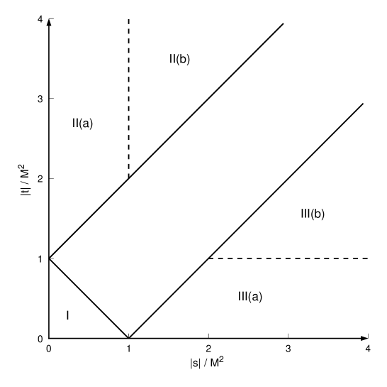
Figure 2: The kinematic regions for the one-loop box with one off-shell leg. The solid line shows the phase-space boundary $|s|+|t|=M^{2}$, together with the reflections $|s|=|t|+M^{2}$ and $|t|=|s|+M^{2}$. The reflections are relevant for the convergence properties of the hypergeometric functions which only involve the absolute values of ratios of the scales. The dashed lines show the boundaries $|s|=M^{2}$ and $|t|=M^{2}$.

$$\begin{array}[]{ll}{\rm region\ I:}&\displaystyle{M^{2}>|s|+|t|,\vspace{1mm}}\\ {\rm region\ II(a):}&\displaystyle{|t|>M^{2}+|s|{\rm\ and\ }M^{2}>|s|,\vspace{1mm}}\\ {\rm region\ II(b):}&\displaystyle{|t|>M^{2}+|s|{\rm\ and\ }|s|>M^{2},\vspace{1mm}}\\ {\rm region\ III(a):}&\displaystyle{|s|>M^{2}+|t|{\rm\ and\ }M^{2}>|t|,\vspace{1mm}}\\ {\rm region\ III(b):}&\displaystyle{|s|>M^{2}+|t|{\rm\ and\ }|t|>M^{2},}\end{array}$$

and, applying the convergence criteria of Table 1 to each of the fifteen solutions, we find that they are distributed as follows:

$$\rm in~{}region~{}I$$

$$I_{4}^{D}(\nu_{1},\nu_{2},\nu_{3},\nu_{4};s,t,M^{2}) = I_{4}^{\{q_{1},q_{2}\}}+I_{4}^{\{p_{1},p_{4}\}}+I_{4}^{\{p_{4},q_{2}\}}+I_{4}^{\{p_{1},q_{1}\}},$$ (2.20)

$$\rm in~{}region~{}II(a)$$

$$I_{4}^{D}(\nu_{1},\nu_{2},\nu_{3},\nu_{4};s,t,M^{2}) = I_{4}^{\{p_{2},p_{4}\}}+I_{4}^{\{p_{2},q_{1}\}}+I_{4}^{\{p_{4},q_{3}\}}+I_{4}^{\{q_{1},q_{3}\}},$$ (2.21)

$$\rm in~{}region~{}II(b)$$

$$I_{4}^{D}(\nu_{1},\nu_{2},\nu_{3},\nu_{4};s,t,M^{2}) = I_{4}^{\{p_{2},p_{3}\}}+I_{4}^{\{p_{2},q_{3}\}}+I_{4}^{\{p_{4},q_{3}\}}+I_{4}^{\{q_{1},q_{3}\}},$$ (2.22)

$$\rm in~{}region~{}III(a)$$

$$I_{4}^{D}(\nu_{1},\nu_{2},\nu_{3},\nu_{4};s,t,M^{2}) = I_{4}^{\{p_{1},p_{3}\}}+I_{4}^{\{p_{3},q_{2}\}}+I_{4}^{\{p_{1},q_{3}\}}+I_{4}^{\{q_{2},q_{3}\}},$$ (2.23)

$$\rm in~{}region~{}III(b)$$

$$I_{4}^{D}(\nu_{1},\nu_{2},\nu_{3},\nu_{4};s,t,M^{2}) = I_{4}^{\{p_{2},p_{3}\}}+I_{4}^{\{p_{3},q_{3}\}}+I_{4}^{\{p_{1},q_{3}\}}+I_{4}^{\{q_{2},q_{3}\}}.\phantom{aaaaaaa}$$ (2.24)

Some solutions are convergent in more than one region. For example, $I_{4}^{\{p_{4},q_{3}\}}$ and $I_{4}^{\{q_{1},q_{3}\}}$ are convergent in both regions II(a) and II(b) while $I_{4}^{\{p_{2},p_{3}\}}$ is convergent in both II(b) and III(b). We also see that in region II(a), two of the solutions $\left(I_{4}^{\{p_{2},p_{4}\}}\right.$ and $\left.I_{4}^{\{p_{4},q_{3}\}}\right)$ contain dangerous $\Gamma$ functions when $\nu_{2}=\nu_{4}$. These divergences indicate the region of a logarithmic analytic continuation and can be regulated by letting $\nu_{2}=\nu_{4}+\delta$, canceling the divergence, and then setting $\delta\,\mbox{$\rightarrow$}\,0$. Similarly, the two divergent contributions in region II(b) $\left(I_{4}^{\{p_{2},q_{3}\}}\right.$ and $\left.I_{4}^{\{p_{4},q_{3}\}}\right)$ also cancel in this limit.

We can perform several checks of these results.

• Analytic continuation
  The solutions in the different regions are related by analytic continuations of the hypergeometric functions (see for example the appendix of Ref. [11]).

• The $\boldsymbol{\nu_{i}=0}$ limit
  By pinching out one or more of the propagators (which corresponds to setting $\nu_{i}=0$) we obtain results for triangle or bubble integrals (see Ref. [11]). For example, if we set $\nu_{2}=\nu_{3}=0$, then any term containing $1/\Gamma(\nu_{2})$ or $1/\Gamma(\nu_{3})$ is eliminated. In fact, only five solutions survive, one in each group. In each case, the hypergeometric function collapses to unity and we obtain the expected result for the massless-bubble integral with off-shellness $M^{2}$ in each of the five kinematic regions thereby spanning the whole of phase space

  $$I_{2}^{D}\left(\nu_{1},\nu_{4};M^{2}\right)=\left(M^{2}\right)^{\frac{D}{2}-\nu_{1}-\nu_{4}}\Pi^{D}(\nu_{1},\nu_{4}),$$ (2.25)

  where we have defined, for future reference,

  $$\Pi^{D}(\mu,\mu^{\prime})=(-1)^{\frac{D}{2}}~{}\frac{\Gamma\left({\mu+\mu^{\prime}-\frac{D}{2}}\right)\Gamma\left({\frac{D}{2}-\mu}\right)\Gamma\left({\frac{D}{2}-\mu^{\prime}}\right)}{\Gamma\left({\mu}\right)\Gamma\left({\mu^{\prime}}\right)\Gamma\left({D-\mu-\mu^{\prime}}\right)}.$$ (2.26)

• The massless box: $\boldsymbol{I_{4}^{D}\left(\nu_{1},\nu_{2},\nu_{3},\nu_{4};s,t,0\right)}$

  The limit $M^{2}\,\mbox{$\rightarrow$}\,0$ can be taken whenever the kinematic region allows it, that is to say, in regions II(b) and III(b), where $M^{2}<|s|$, $M^{2}<|t|$. These two regions are related by the symmetry $\left(s\leftrightarrow t,\ \nu_{1}\leftrightarrow\nu_{4},\ \nu_{2}\leftrightarrow\nu_{3}\right)$, so we focus only on region II(b). Only three of the solutions survive, and we have:

  $${\rm if\ }|s|<|t|\hskip 42.67912pt$$

  $$I_{4}^{D}\left(\nu_{1},\nu_{2},\nu_{3},\nu_{4};s,t,0\right)=\left.I_{4}^{\{q_{1},q_{3}\}}\right|_{M^{2}=0}+\left.I_{4}^{\{p_{2},q_{3}\}}\right|_{M^{2}=0}+\left.I_{4}^{\{p_{4},q_{3}\}}\right|_{M^{2}=0}$$ (2.27)

  $$= (-1)^{\frac{D}{2}}~{}t^{\frac{D}{2}-\sigma}\frac{\Gamma\left(\sigma-\frac{D}{2}\right)\Gamma\left(\frac{D}{2}-\nu_{134}\right)\Gamma\left(\frac{D}{2}-\nu_{123}\right)}{\Gamma\left(\nu_{2}\right)\Gamma\left(\nu_{4}\right)\Gamma\left(D-\sigma\right)}$$

  $$\times~{}~{}~{}{{}_{3}F_{2}}\left(\nu_{1},\nu_{3},\sigma-\frac{D}{2},1+\nu_{134}-\frac{D}{2},1+\nu_{123}-\frac{D}{2},-\frac{s}{t}\right)$$

  $$+ (-1)^{\frac{D}{2}}~{}s^{\frac{D}{2}-\nu_{123}}t^{-\nu_{4}}\frac{\Gamma\left(\nu_{123}-\frac{D}{2}\right)\Gamma\left(\nu_{2}-\nu_{4}\right)\Gamma\left(\frac{D}{2}-\nu_{23}\right)\Gamma\left(\frac{D}{2}-\nu_{12}\right)}{\Gamma\left(\nu_{1}\right)\Gamma\left(\nu_{2}\right)\Gamma\left(\nu_{3}\right)\Gamma\left(D-\sigma\right)}$$

  $$\times~{}~{}~{}{{}_{3}F_{2}}\left(\nu_{4},\frac{D}{2}-\nu_{12},\frac{D}{2}-\nu_{23},1+\nu_{4}-\nu_{2},1+\frac{D}{2}-\nu_{123},-\frac{s}{t}\right)$$

  $$+ (-1)^{\frac{D}{2}}~{}s^{\frac{D}{2}-\nu_{134}}t^{-\nu_{2}}\frac{\Gamma\left(\nu_{134}-\frac{D}{2}\right)\Gamma\left(\nu_{4}-\nu_{2}\right)\Gamma\left(\frac{D}{2}-\nu_{14}\right)\Gamma\left(\frac{D}{2}-\nu_{34}\right)}{\Gamma\left(\nu_{1}\right)\Gamma\left(\nu_{3}\right)\Gamma\left(\nu_{4}\right)\Gamma\left(D-\sigma\right)}$$

  $$\times~{}~{}~{}{{}_{3}F_{2}}\left(\nu_{2},\frac{D}{2}-\nu_{14},\frac{D}{2}-\nu_{34},1-\nu_{4}+\nu_{2},1+\frac{D}{2}-\nu_{134},-\frac{s}{t}\right).$$

  Similarly, taking the same $M^{2}\,\mbox{$\rightarrow$}\,0$ limit for solution (2.24) in region III(b), we find the result valid when $|s|>|t|$, which is also obtained by applying the exchanges $(s\leftrightarrow t$, $\nu_{1}\leftrightarrow\nu_{4}$, $\nu_{2}\leftrightarrow\nu_{3})$ to Eq. (- ‣ 2). Note that we could have obtained the same result by returning to the template solution (2.11) with the system of constraints (2) and, after setting $q_{3}=0$, solved the on-shell box directly. In this case, there are two external scales, $s$ and $t$, so that there will be six summation variables ($p_{1},\ldots,p_{4}$ and $q_{1}$, $q_{2}$) and five constraints yielding six solutions, three of which converge when $|s|<|t|$, again yielding Eq. (- ‣ 2).

  As before, there are apparent divergences in the $\Gamma$ functions when $\nu_{2}=\nu_{4}$ that must be regulated. This is straightforwardly achieved for particular values of the parameters by setting $\nu_{2}=\nu_{4}+\delta$ and making a Taylor expansion.

• The $\boldsymbol{\nu_{i}=1}$ limit: $\boldsymbol{I_{4}^{D}(1,1,1,1;s,t,M^{2})}$

  If we set the propagator power equal to one, then all the groups (2.20)–(2.24) give the correct answer

  $$I_{4}^{D}(1,1,1,1;s,t,M^{2})=\frac{2}{\epsilon^{2}}\frac{\Gamma^{2}\left(1-\epsilon\right)\Gamma\left({1+\epsilon}\right)}{\Gamma\left({1-2\epsilon}\right)}\frac{1}{st}\Biggl{[}(-t)^{-\epsilon}{{}_{2}F_{1}}\left(1,-\epsilon,1-\epsilon,-\frac{u}{s}\right)\hskip 22.76228pt$$

  $$\hskip 56.9055pt+(-s)^{-\epsilon}{{}_{2}F_{1}}\left(1,-\epsilon,1-\epsilon,-\frac{u}{t}\right)-(-M^{2})^{-\epsilon}{{}_{2}F_{1}}\left(-\epsilon,1,1-\epsilon,-\frac{M^{2}u}{st}\right)\Biggr{]},$$

  where $u$ is defined by $s+t+u=M^{2}$ and $\epsilon=(4-D)/2$. To obtain this result we have returned to the series representation of the hypergeometric function and manipulated the series by repeatedly summing with respect to one summation index to obtain an ${{}_{2}F_{1}}$ function, applied identities to change the arguments of the ${{}_{2}F_{1}}$ and rewritten the ${{}_{2}F_{1}}$ as a series. Then we sum with respect to the other index, and repeat if necessary. Eventually all of the hypergeometric functions of two variables can be reduced to ${{}_{2}F_{1}}$ functions.

3 Application to two-loop box graphs

Figure 3: A one-loop insertion into a one-loop box diagram.

The general results for one-loop box graphs presented in the previous section may be applied to give analytic results for two-loop box integrals when there are one-loop insertions on one of the propagators. As is well known, the effect of such insertions is to modify the power to which that propagator is raised. For example, we consider the two-loop integral shown in Fig. 3, with off-shell legs

$$J^{D}_{4}\left(\mu_{1},\mu_{2},\mu_{3},\{\mu_{4},\mu_{5},\mu_{6},\mu_{7}\};\{Q_{i}^{2}\}\right)=\int\frac{d^{D}k}{i\pi^{D/2}}\int\frac{d^{D}l}{i\pi^{D/2}}\frac{1}{A_{1}^{\mu_{1}}A_{2}^{\mu_{2}}A_{3}^{\mu_{3}}A_{4}^{\mu_{4}}B_{1}^{\mu_{5}}B_{2}^{\mu_{6}}A_{4}^{\mu_{7}}},$$ (3.1)

where the $A_{i}$ are independent of the second loop momentum $l$ and are given by Eq. (2) while

$$B_{1} = l^{2}+i0$$

$$B_{2} = (l+k+k_{1}+k_{2}+k_{3})^{2}+i0.$$ (3.2)

The momentum flowing through the bubble is $k+k_{1}+k_{2}+k_{3}$ so that the result of the integration over $l$ is (see Eq. (2.25))

$$\int\frac{d^{D}l}{i\pi^{D/2}}\frac{1}{B_{1}^{\mu_{5}}B_{2}^{\mu_{6}}}=I_{2}^{D}\left(\mu_{5},\mu_{6};A_{4}\right)=\Pi^{D}(\mu_{5},\mu_{6})~{}A_{4}^{\frac{D}{2}-\mu_{5}-\mu_{6}},$$ (3.3)

where $\Pi^{D}$ is defined in Eq. (2.26). In this way, the overall power to which $A_{4}$ is raised to, in the two-loop diagram (3.1), is $\mu_{4}+\mu_{5}+\mu_{6}+\mu_{7}-\frac{D}{2}$. Inserting Eq. (3.3) into (3.1) we find

$$J^{D}_{4}\left(\mu_{1},\mu_{2},\mu_{3},\{\mu_{4},\mu_{5},\mu_{6},\mu_{7}\};\{Q_{i}^{2}\}\right)=\Pi^{D}(\mu_{5},\mu_{6})~{}I_{4}^{D}\left(\mu_{1},\mu_{2},\mu_{3},\mu_{4567}-\frac{D}{2};\{Q_{i}^{2}\}\right),$$ (3.4)

where $\mu_{4567}=\mu_{4}+\mu_{5}+\mu_{6}+\mu_{7}$. Results for diagrams obtained by pinching out one of the propagators are obtained by setting the corresponding $\mu_{i}\,\mbox{$\rightarrow$}\,0$. For example, one of the boundary integrals of Ref. [4] is obtained as the special case of (3.4), with $\mu_{4}=\mu_{7}=0$ (see Fig. 4 (a)). Similarly, the two-loop diagrams with one-loop insertions on the other three propagators are defined in an analogous way so that

$$J^{D}_{4}\left(\{\mu_{1},\mu_{2},\mu_{3},\mu_{4}\},\mu_{5},\mu_{6},\mu_{7};\{Q_{i}^{2}\}\right) = \Pi^{D}(\mu_{2},\mu_{3})~{}I_{4}^{D}\left(\mu_{1234}-\frac{D}{2},\mu_{5},\mu_{6},\mu_{7};\{Q_{i}^{2}\}\right),$$

$$J^{D}_{4}\left(\mu_{1},\{\mu_{2},\mu_{3},\mu_{4},\mu_{5}\},\mu_{6},\mu_{7};\{Q_{i}^{2}\}\right) = \Pi^{D}(\mu_{3},\mu_{4})~{}I_{4}^{D}\left(\mu_{1},\mu_{2345}-\frac{D}{2},\mu_{6},\mu_{7};\{Q_{i}^{2}\}\right),$$

$$J^{D}_{4}\left(\mu_{1},\mu_{2},\{\mu_{3},\mu_{4},\mu_{5},\mu_{6}\},\mu_{7};\{Q_{i}^{2}\}\right) = \Pi^{D}(\mu_{4},\mu_{5})~{}I_{4}^{D}\left(\mu_{1},\mu_{2},\mu_{3456}-\frac{D}{2},\mu_{7};\{Q_{i}^{2}\}\right),$$

where the notation is obvious.

For box graphs with only one off-shell leg, the symmetry of the diagram reduces the number of distinct integrals to two:

$$J^{D}_{4}\left(\{\mu_{1},\mu_{2},\mu_{3},\mu_{4}\},\mu_{5},\mu_{6},\mu_{7};s,t,M^{2}\right) = J^{D}_{4}\left(\mu_{7},\mu_{6},\mu_{5},\{\mu_{4},\mu_{3},\mu_{2},\mu_{1}\};t,s,M^{2}\right),$$ (3.6)

$$J^{D}_{4}\left(\mu_{1},\{\mu_{2},\mu_{3},\mu_{4},\mu_{5}\},\mu_{6},\mu_{7};s,t,M^{2}\right) = J^{D}_{4}\left(\mu_{7},\mu_{6},\{\mu_{5},\mu_{4},\mu_{3},\mu_{2}\},\mu_{1};t,s,M^{2}\right),\phantom{aaa}$$ (3.7)

so that it is sufficient to consider diagrams with insertions on the third and fourth propagators. In the on-shell limit $(M^{2}\,\mbox{$\rightarrow$}\,0)$, there is the further relation

$$J^{D}_{4}\left(\mu_{1},\mu_{2},\{\mu_{3},\mu_{4},\mu_{5},\mu_{6}\},\mu_{7};s,t\right)=J^{D}_{4}\left(\mu_{7},\mu_{1},\mu_{2},\{\mu_{3},\mu_{4},\mu_{5},\mu_{6}\};t,s\right),$$ (3.8)

so that for the massless box we only need to consider insertions on a single propagator.

3.1 One-loop insertions in the one-loop box with one off-shell leg

In this section, we further specify the values of the propagators in the general forms for the one-loop box graphs of Eqs. (2.20)–(2.24): we fix three of the propagator powers equal to one, while the fourth power is kept free. Because of the symmetry properties of the integral (3.6), we need only to keep either $\nu_{4}$ or $\nu_{3}$ general.

• $\boldsymbol{I_{4}^{D}\left(1,1,1,\nu_{4};s,t,M^{2}\right)}$
  This limit is appropriate for two-loop diagrams such as that depicted in Fig. 3. We choose to work with the solutions in region I, given by Eq. (2.20). Each of the four solutions is an Appell $F_{2}$ function which can be represented as a double Eulerian integral (see Eq. (A.12)). However, for this choice of the parameters, the $F_{2}$ functions simplify (see Refs. [11, 14, 16]) and we find

  $$I_{4}^{D}\left(1,1,1,\nu_{4};s,t,M^{2}\right)$$ (3.9)

  $$= (-1)^{\frac{D}{2}}~{}\left(M^{2}\right)^{\frac{D}{2}-2-\nu_{4}}\left(M^{2}-t\right)^{-1}\frac{\Gamma\left({3+\nu_{4}-\frac{D}{2}}\right)\Gamma\left({\frac{D}{2}-3}\right)\Gamma\left({\frac{D}{2}-2-\nu_{4}}\right)}{\Gamma\left({\nu_{4}}\right)\Gamma\left({D-3-\nu_{4}}\right)}$$

  $$\times~{}~{}~{}F_{1}\left(1,2+\nu_{4}-\frac{D}{2},1,4-\frac{D}{2},\frac{s}{M^{2}},\frac{s}{M^{2}-t}\right)$$

  $$+ (-1)^{\frac{D}{2}}~{}s^{\frac{D}{2}-3}t^{\frac{D}{2}-2-\nu_{4}}\left(M^{2}-s-t\right)^{2-\frac{D}{2}}$$

  $$\times~{}~{}~{}\frac{\Gamma\left({3-\frac{D}{2}}\right)\Gamma\left({2+\nu_{4}-\frac{D}{2}}\right)\Gamma\left({\frac{D}{2}-2}\right)^{2}\Gamma\left({\frac{D}{2}-1-\nu_{4}}\right)}{\Gamma\left({\nu_{4}}\right)\Gamma\left({D-3-\nu_{4}}\right)}$$

  $$+ (-1)^{\frac{D}{2}}~{}t^{\frac{D}{2}-2-\nu_{4}}\left(M^{2}-t\right)^{-1}\frac{\Gamma\left({2+\nu_{4}-\frac{D}{2}}\right)\Gamma\left({\frac{D}{2}-3}\right)\Gamma\left({\frac{D}{2}-1-\nu_{4}}\right)}{\Gamma\left({\nu_{4}}\right)\Gamma\left({D-3-\nu_{4}}\right)}$$

  $$\times~{}~{}~{}{{}_{2}F_{1}}\left(1,1,4-\frac{D}{2},\frac{s}{M^{2}-t}\right)$$

  $$+ (-1)^{\frac{D}{2}}~{}s^{\frac{D}{2}-3}\left(M^{2}-s\right)^{-\nu_{4}}\frac{\Gamma\left({3-\frac{D}{2}}\right)\Gamma\left({\frac{D}{2}-2}\right)\Gamma\left({\frac{D}{2}-2-\nu_{4}}\right)}{\Gamma\left({D-3-\nu_{4}}\right)}$$

  $$\times~{}~{}~{}{{}_{2}F_{1}}\left(1,\nu_{4},3+\nu_{4}-\frac{D}{2},\frac{t}{M^{2}-s}\right).$$

  Note that the value of $D$ plays no role in simplifying the hypergeometric functions and the result given here is for general $D$. The remaining hypergeometric functions can now be manipulated using standard identities and the one-dimensional integral representations given in Sec. A.2 can be used for specific evaluations. At this stage, a series expansion in $\epsilon=(4-D)/2$ becomes necessary.

• $\boldsymbol{I_{4}^{D}\left(1,1,\nu_{3},1;s,t,M^{2}\right)}$
  Similarly, for the case where $\nu_{1}=\nu_{2}=\nu_{4}=1$ and $\nu_{3}$ is kept general, we obtain

  $$I_{4}^{D}\left(1,1,\nu_{3},1;s,t,M^{2}\right)$$ (3.10)

  $$= (-1)^{\frac{D}{2}}~{}\left(M^{2}\right)^{\frac{D}{2}-2}\left(M^{2}-s\right)^{-\nu_{3}}\left(M^{2}-t\right)^{-1}\frac{\Gamma\left({3+\nu_{3}-\frac{D}{2}}\right)\Gamma\left({\frac{D}{2}-2-\nu_{3}}\right)^{2}}{\Gamma\left({D-3-\nu_{3}}\right)}$$

  $$\times~{}~{}~{}{{}_{2}F_{1}}\left(1,\nu_{3},3+\nu_{3}-\frac{D}{2},\frac{st}{(M^{2}-s)(M^{2}-t)}\right)$$

  $$+ (-1)^{\frac{D}{2}}~{}s^{\frac{D}{2}-2-\nu_{3}}t^{\frac{D}{2}-2-\nu_{3}}\left(M^{2}-s-t\right)^{2-\frac{D}{2}}\left(M^{2}-t\right)^{\nu_{3}-1}$$

  $$\times~{}~{}~{}\frac{\Gamma\left({2+\nu_{3}-\frac{D}{2}}\right)^{2}\Gamma\left({\frac{D}{2}-2}\right)\Gamma\left({\frac{D}{2}-1-\nu_{3}}\right)^{2}}{\Gamma\left({\nu_{3}}\right)\Gamma\left({D-3-\nu_{3}}\right)}$$

  $$+ (-1)^{\frac{D}{2}}~{}t^{\frac{D}{2}-2-\nu_{3}}\left(M^{2}-t\right)^{-1}\frac{\Gamma\left({2+\nu_{3}-\frac{D}{2}}\right)\Gamma\left({\frac{D}{2}-2-\nu_{3}}\right)\Gamma\left({\frac{D}{2}-1-\nu_{3}}\right)}{\Gamma\left({D-3-\nu_{3}}\right)}$$

  $$\times~{}~{}~{}{{}_{2}F_{1}}\left(1,\nu_{3},3+\nu_{3}-\frac{D}{2},\frac{s}{M^{2}-t}\right)$$

  $$+ (-1)^{\frac{D}{2}}~{}s^{\frac{D}{2}-2-\nu_{3}}\left(M^{2}\right)^{-1}\frac{\Gamma\left({2+\nu_{3}-\frac{D}{2}}\right)\Gamma\left({\frac{D}{2}-2}\right)\Gamma\left({\frac{D}{2}-2-\nu_{3}}\right)}{\Gamma\left({\nu_{3}}\right)\Gamma\left({D-3-\nu_{3}}\right)}$$

  $$\times~{}~{}~{}{F_{2}}\left(1,\frac{D}{2}-2,1,\frac{D}{2}-1-\nu_{3},3+\nu_{3}-\frac{D}{2},\frac{s}{M^{2}},\frac{t}{M^{2}}\right).$$

  In this case, one $F_{2}$ function does not reduce simply and it is necessary to resort to the two-dimensional integral representation of Eq. (A.12) for explicit evaluation.

3.2 One-loop insertions in the massless one-loop box

We can also attack the problem in the on-shell box. Here we set $\nu_{1}=\nu_{2}=\nu_{3}=1$ and keep $\nu_{4}$ general, which is appropriate for diagrams such as those shown in Figs. 3 and 4. Insertions on the other legs are given by the symmetry properties of the integral (see Eqs. (3.6)–(3.8)). We therefore choose to work with the solution valid when $|s|<|t|$ since that contains no $\Gamma$ functions that are singular when $\nu_{1}=\nu_{3}$. In every case, the ${{}_{3}F_{2}}$ functions of Eq. (- ‣ 2) reduce to ${{}_{2}F_{1}}$ functions and we find

$$I_{4}^{D}\left(1,1,1,\nu_{4};s,t\right) = (-1)^{\frac{D}{2}}~{}t^{\frac{D}{2}-3-\nu_{4}}\frac{\Gamma\left(3+\nu_{4}-\frac{D}{2}\right)\Gamma\left(\frac{D}{2}-2-\nu_{4}\right)\Gamma\left(\frac{D}{2}-3\right)}{\Gamma\left(\nu_{4}\right)\Gamma\left(D-3-\nu_{4}\right)}$$ (3.11)

$$\times~{}~{}~{}{{}_{2}F_{1}}\left(1,1,4-\frac{D}{2},-\frac{s}{t}\right)$$

$$+ (-1)^{\frac{D}{2}}~{}s^{\frac{D}{2}-2-\nu_{4}}t^{-1}\frac{\Gamma\left(2+\nu_{4}-\frac{D}{2}\right)\Gamma\left(\nu_{4}-1\right)\Gamma\left(\frac{D}{2}-1-\nu_{4}\right)^{2}}{\Gamma\left(\nu_{4}\right)\Gamma\left(D-3-\nu_{4}\right)}$$

$$\times~{}~{}~{}{{}_{2}F_{1}}\left(1,\frac{D}{2}-1-\nu_{4},2-\nu_{4},-\frac{s}{t}\right)$$

$$+ (-1)^{\frac{D}{2}}~{}s^{\frac{D}{2}-3}t^{-\nu_{4}}\frac{\Gamma\left(3-\frac{D}{2}\right)\Gamma\left(1-\nu_{4}\right)\Gamma\left(\frac{D}{2}-2\right)^{2}}{\Gamma\left(D-3-\nu_{4}\right)}$$

$$\times~{}~{}~{}\left(1+\frac{s}{t}\right)^{2-\frac{D}{2}}.$$

There is still an apparent divergence as $\nu_{4}\,\mbox{$\rightarrow$}\,1$ which can be easily removed by manipulating the hypergeometric functions using the well known analytic continuations to obtain

$$I_{4}^{D}\left(1,1,1,\nu_{4};s,t\right)\!\! = \!\!(-1)^{\frac{D}{2}}~{}t^{\frac{D}{2}-2-\nu_{4}}s^{-1}\frac{\Gamma\left(3+\nu_{4}-\frac{D}{2}\right)\Gamma\left({\frac{D}{2}-2}\right)\Gamma\left({2-\frac{D}{2}}\right)\Gamma\left(\frac{D}{2}-2-\nu_{4}\right)}{\Gamma\left(\nu_{4}\right)\Gamma\left(D-3-\nu_{4}\right)\Gamma\left({3-\frac{D}{2}}\right)}$$ (3.12)

$$\times~{}~{}~{}{{}_{2}F_{1}}\left(1,\frac{D}{2}-2,\frac{D}{2}-1,\frac{s+t}{s}\right)$$

$$+ \!\!(-1)^{\frac{D}{2}}~{}s^{\frac{D}{2}-3-\nu_{4}}\frac{\Gamma\left({2+\nu_{4}-\frac{D}{2}}\right)\Gamma\left({\frac{D}{2}-\nu_{4}-1}\right)^{2}\Gamma\left({2-\frac{D}{2}}\right)}{\Gamma\left({D-3-\nu_{4}}\right)\Gamma\left({3-\frac{D}{2}}\right)}$$

$$\times~{}~{}~{}{{}_{2}F_{1}}\left(1,\nu_{4},\frac{D}{2}-1,\frac{s+t}{s}\right).$$

We have checked that the same result can be obtained by starting from the general solution valid for $|t|<|s|$. In this case, we must regulate the singularity as $\nu_{3}\,\mbox{$\rightarrow$}\,\nu_{1}$ by setting $\nu_{3}=\nu_{1}+\delta$. The singularity as $\delta\,\mbox{$\rightarrow$}\,0$ is canceled by analytically continuing the ${{}_{2}F_{1}}$’s and, after taking the $\delta\,\mbox{$\rightarrow$}\,0$ limit, we recover Eq. (3.12).

(a)   (b)  

Figure 4: Two-loop box diagrams with pinched propagators.

3.2.1 Explicit evaluation of two-loop box integrals

To give more explicit expressions requires a more precise knowledge of $\nu_{4}$. For the two-loop diagram shown in Fig. 3 the value of $\nu_{4}$ is given by $\mu_{4}+\mu_{5}+\mu_{6}+\mu_{7}-\frac{D}{2}=n-\frac{D}{2}$, where $n$ is an integer. The case $n=2$ corresponds to the simplest case $\mu_{4}=\mu_{7}=0$ and $\mu_{5}=\mu_{6}=1$, shown in Fig. 4 (a). Substituting this value in the general expression (3.12) and restoring all overall factors, we find that the expression for this two-loop integral in $D=4-2\epsilon$ is given by (see Eq. (3.4))

$$J_{4}^{D}(1,1,1,\{0,1,1,0\};s,t) = \left(-t\right)^{-2\epsilon}\frac{K_{1}}{2\,s\,\epsilon^{3}}~{}{{}_{2}F_{1}}\left(1,-\epsilon,1-\epsilon,\frac{s+t}{s}\right)$$ (3.13)

$$+ \left(-s\right)^{-2\epsilon}\frac{K_{2}}{2\,s\,\epsilon^{3}}~{}{{}_{2}F_{1}}\left(1,\epsilon,1-\epsilon,\frac{s+t}{s}\right),$$

where the constants $K_{1}$ and $K_{2}$ are given by

$$K_{1} = \frac{\Gamma\left({1+2\epsilon}\right)\Gamma\left({1-\epsilon}\right)^{3}}{\left(1-2\epsilon\right)\Gamma\left({1-3\epsilon}\right)}$$ (3.14)

$$K_{2} = \frac{\Gamma\left({1+2\epsilon}\right)\Gamma\left({1-2\epsilon}\right)\Gamma\left({1+\epsilon}\right)\Gamma\left({1-\epsilon}\right)^{2}}{\left(1-2\epsilon\right)\Gamma\left({1-3\epsilon}\right)}.$$ (3.15)

Note that by starting off with the NDIM approach, we have not actually had to perform any integrations to reach this result or make any assumptions about the smallness of $\epsilon$. The hypergeometric functions have one-dimensional integral representations (see Eq. (A.10)) and can be expanded around $\epsilon=0$ in terms of polylogarithms. The necessary integrals are easily done

$${{}_{2}F_{1}}\left(1,-\epsilon,1-\epsilon,x\right)=1+\epsilon\log(1-x)-\epsilon^{2}\,{\rm Li}_{2}\left(x\right)-\epsilon^{3}\,{\rm Li}_{3}\left(x\right)+{\cal O}\left(\epsilon^{4}\right)$$ (3.16)

$${{}_{2}F_{1}}\left(1,\epsilon,1-\epsilon,x\right)=1-\epsilon\log(1-x)+\epsilon^{2}\left[-2\,{\rm Li}_{2}\left(\frac{x}{x-1}\right)-\,{\rm Li}_{2}\left(x\right)\right]$$

$$\phantom{{{}_{2}F_{1}}\left(1,\epsilon,1-\epsilon,\right)\,\,\,\,}-\epsilon^{3}\left[2\,{\rm Li}_{3}\left(\frac{x}{x-1}\right)+\,{\rm Li}_{3}\left(x\right)+\frac{1}{3}\log^{3}(1-x)\right]\!+{\cal O}\left(\epsilon^{4}\right),$$ (3.17)

where the polylogarithms are defined by

$$\,{\rm Li}_{2}\left(x\right)=-\int_{0}^{x}dz\,\frac{\log(1-z)}{z}\hskip 28.45274ptx\leq 1\;,$$ (3.18)

and

$$\,{\rm Li}_{3}\left(x\right)=\int_{0}^{1}dz\,\frac{\log(z)\log(1-xz)}{z}=\int_{0}^{x}dz\,\frac{\,{\rm Li}_{2}\left(z\right)}{z}\hskip 28.45274ptx\leq 1\;.$$ (3.19)

For $x>1$, the following analytic continuations should be used

$$\,{\rm Li}_{2}\left(x\pm i0\right) = -\,{\rm Li}_{2}\left(\frac{1}{x}\right)-\frac{1}{2}\log^{2}x+\frac{\pi^{2}}{3}\pm i\pi\log x\hskip 28.45274ptx>1\;,$$ (3.20)

$$\,{\rm Li}_{3}\left(x\pm i0\right) = \,{\rm Li}_{3}\left(\frac{1}{x}\right)-\frac{1}{6}\log^{3}(x)+\frac{\pi^{2}}{3}\log(x)\pm i\frac{\pi}{2}\log^{2}(x)\hskip 28.45274ptx>1\;.$$ (3.21)

Similarly, the integral with only one pinched propagator, $\mu_{4}=\mu_{5}=\mu_{6}=1$ and $\mu_{7}=0$, shown in Fig. 4 (b) is given by

$$J_{4}^{D}(1,1,1,\{1,1,1,0\};s,t) = \left(-t\right)^{-2\epsilon}\frac{3\,K_{1}}{2\,s\,t\,\epsilon^{3}}~{}{{}_{2}F_{1}}\left(1,-\epsilon,1-\epsilon,\frac{s+t}{s}\right)$$ (3.22)

$$- \left(-s\right)^{-2\epsilon}\frac{3\,K_{2}}{4\,s^{2}\,\epsilon^{3}}~{}{{}_{2}F_{1}}\left(1,1+\epsilon,1-\epsilon,\frac{s+t}{s}\right).$$

The series expansion for the first hypergeometric function is given by Eq. (3.16) while the second can be obtained from Eq. (3.2.1) by using Gauss’s relation between contiguous hypergeometric functions

$$(\beta-\alpha)(1-x)\,{{}_{2}F_{1}}(\alpha,\beta,\gamma,x)-(\gamma-\alpha)\,{{}_{2}F_{1}}(\alpha-1,\beta,\gamma,x)+(\gamma-\beta)\,{{}_{2}F_{1}}(\alpha,\beta-1,\gamma,x)=0,$$ (3.23)

such that

$${{}_{2}F_{1}}(1,\beta+1,1-\epsilon,x)=-\frac{\epsilon}{\beta(1-x)}+\frac{(\epsilon+\beta)}{\beta(1-x)}\,{{}_{2}F_{1}}(1,\beta,1-\epsilon,x).$$ (3.24)

Finally, the scalar integral for the bubble insertion $\mu_{4}=\mu_{5}=\mu_{6}=\mu_{7}=1$ shown in Fig. 3 is

$$J_{4}^{D}(1,1,1,\{1,1,1,1\};s,t) = \left(-t\right)^{-2\epsilon}\frac{3\,(1+3\epsilon)\,K_{1}}{2\,(1+\epsilon)\,s\,t^{2}\,\epsilon^{3}}~{}{{}_{2}F_{1}}\left(1,-\epsilon,1-\epsilon,\frac{s+t}{s}\right)$$ (3.25)

$$+ \left(-s\right)^{-2\epsilon}\frac{3\,(1+3\epsilon)\,K_{2}}{4\,(1+2\epsilon)\,s^{3}\,\epsilon^{3}}~{}{{}_{2}F_{1}}\left(1,2+\epsilon,1-\epsilon,\frac{s+t}{s}\right).\phantom{aaa}$$

Once again, the series expansion for the first hypergeometric function is given by Eq. (3.16) while the second can be obtained from Eq. (3.2.1) by repeated use of Eq. (3.24).

4 Conclusions

In this paper we have evaluated one-loop massless box integrals with arbitrary powers of the propagators and with up to one off-shell leg as combinations of hypergeometric functions. The method we have used, first suggested by Halliday and Ricotta, has its roots in the analytic properties of loop integrals and, in particular, the possibility of treating the space-time dimensions $D$ as a negative integer in intermediate steps. In Ref. [11] we have developed a general strategy for evaluating one-loop integrals in NDIM and we have pointed out some subtleties that can occur in the application of the method. For the box integrals we have considered here, with $q$ energy scales, we have expressed the final result as finite sums of hypergeometric functions with $q-1$ variables, that converge in the appropriate kinematic regions. The general results for one off-shell leg in the kinematic regions specified by Eq. (2) are given in Eqs. (2.20)–(2.24). Similar expressions for the on-shell case are given in Eq. (- ‣ 2). We would like to point out that no integration was actually necessary in obtaining these results.

All of these expressions are valid for arbitrary powers of the propagators and are therefore relevant to classes of multiloop graphs where there are (multiple) one-loop insertions on the propagators. We have studied how these expressions are relevant to this type of two-loop graph and, in particular, two-loop graphs with three powers of propagators set to unity and one propagator (corresponding to the place where the one-loop insertion is made) kept arbitrary. With this choice of parameters, identities amongst hypergeometric functions can be used to simplify the general expressions. Explicit results in terms of hypergeometric functions are given for the one off-shell case in Eqs. (3.9) and (3.10). In the on-shell case, the two-loop scalar integrals reduce down to two Gaussian ${{}_{2}F_{1}}$ functions. Up to this point we have not actually had to perform any integrations explicitly or make a series expansion in $\epsilon=(4-D)/2$. However, to write the hypergeometric integrals in terms of logarithms and polylogarithms it is necessary to use an integral representation and make the series expansion in $\epsilon$. For the ${{}_{2}F_{1}}$ functions, the integral representation is one-dimensional and the integrals are well known. Explicit results for the graphs of Figs. 3 and 4 are given in Eqs. (3.13), (3.22) and (3.25).

It is clear that NDIM is an extremely efficient way of solving one-loop integrals. Furthermore, as we have shown in this paper and as Suzuki and Schmidt [6, 7] have previously shown, NDIM can help in evaluating multi-loop integrals where there are one-loop insertions on one or more of the propagators. Whether or not NDIM can provide some non-trivial results for multi-loop graphs is an interesting, but still open, question.

A Hypergeometric definitions and identities

In Sec. A.1 we give the definitions of the hypergeometric functions as a series together with their regions of convergence. Integral representations for the ${{}_{2}F_{1}}$, $F_{1}$ and $F_{2}$ functions are given in Sec. A.2 while identities for reducing the $F_{1}$ and $F_{2}$ functions to simpler functions are given in Sec. A.3.

A.1 Series representations

The hypergeometric functions of one variable are sums of Pochhammer symbols over a single summation parameter $m$

$${{}_{2}F_{1}}\left(\alpha,\beta,\gamma,x\right) = \sum_{m=0}^{\infty}\frac{(\alpha,m)(\beta,m)}{(\gamma,m)}\,\frac{x^{m}}{m!}$$ (A.1)

$${{}_{3}F_{2}}\left(\alpha,\beta,\beta^{\prime},\gamma,\gamma^{\prime},x\right) = \sum_{m=0}^{\infty}\frac{(\alpha,m)(\beta,m)(\beta^{\prime},m)}{(\gamma,m)(\gamma^{\prime},m)}\,\frac{x^{m}}{m!},$$ (A.2)

which are convergent when $|x|<1$.

The hypergeometric functions of two variables can be written as sums over the integers $m$ and $n$: $F_{i}$, $i=1,\ldots,4$ are the Appell functions, $H_{2}$ a Horn function and $S_{1}$ and $S_{2}$ generalised Kampé de Fériet functions:

$$F_{1}\left(\alpha,\beta,\beta^{\prime},\gamma,x,y\right) = \sum_{m,n=0}^{\infty}\frac{(\alpha,m+n)(\beta,m)(\beta^{\prime},n)}{(\gamma,m+n)}\,\frac{x^{m}}{m!}\,\frac{y^{n}}{n!}$$ (A.3)

$$F_{2}\left(\alpha,\beta,\beta^{\prime},\gamma,\gamma^{\prime},x,y\right) = \sum_{m,n=0}^{\infty}\frac{(\alpha,m+n)(\beta,m)(\beta^{\prime},n)}{(\gamma,m)(\gamma^{\prime},n)}\,\frac{x^{m}}{m!}\,\frac{y^{n}}{n!}$$ (A.4)

$$F_{3}\left(\alpha,\alpha^{\prime},\beta,\beta^{\prime},\gamma,x,y\right) = \sum_{m,n=0}^{\infty}\frac{(\alpha,m)(\alpha^{\prime},n)(\beta,m)(\beta^{\prime},n)}{(\gamma,m+n)}\,\frac{x^{m}}{m!}\,\frac{y^{n}}{n!}$$ (A.5)

$$F_{4}\left(\alpha,\beta,\gamma,\gamma^{\prime},x,y\right) = \sum_{m,n=0}^{\infty}\frac{(\alpha,m+n)(\beta,m+n)}{(\gamma,m)(\gamma^{\prime},n)}\,\frac{x^{m}}{m!}\,\frac{y^{n}}{n!}$$ (A.6)

$$H_{2}\left(\alpha,\beta,\gamma,\gamma^{\prime},\delta,x,y\right) = \sum_{m,n=0}^{\infty}\frac{(\alpha,m-n)(\beta,m)(\gamma,n)(\gamma^{\prime},n)}{(\delta,m)}\,\frac{x^{m}}{m!}\,\frac{y^{n}}{n!}$$ (A.7)

$$S_{1}\left(\alpha,\alpha^{\prime},\beta,\gamma,\delta,x,y\right) = \sum_{m,n=0}^{\infty}\frac{(\alpha,m+n)(\alpha^{\prime},m+n)(\beta,m)}{(\gamma,m+n)(\delta,m)}\,\frac{x^{m}}{m!}\,\frac{y^{n}}{n!}$$ (A.8)

$$S_{2}\left(\alpha,\alpha^{\prime},\beta,\beta^{\prime},\gamma,x,y\right) = \sum_{m,n=0}^{\infty}\frac{(\alpha,m-n)(\alpha^{\prime},m-n)(\beta,n)(\beta^{\prime},n)}{(\gamma,m-n)}\,\frac{x^{m}}{m!}\,\frac{y^{n}}{n!}.\phantom{aaa}$$ (A.9)

These series converge according to the criteria collected in Table 1.

Function	Convergence criteria
$F_{1}$, $F_{3}$	$\displaystyle{|x|<1},\ |y|<1$
$F_{2}$, $S_{1}$	$\displaystyle{|x|+|y|<1}$
$F_{4}$	$\displaystyle{\sqrt{|x|}+\sqrt{|y|}<1}$
$H_{2}$, $S_{2}$	$-|x|+1/|y|>1$, $|x|<1$, $|y|<1$

Table 1: Convergence regions for some hypergeometric functions of two variables.

The domain of convergence of the Appell and Horn functions are well known. That one for $S_{1}$ and $S_{2}$ may be worked out using Horns general theory of convergence [15].

A.2 Integral representations

Euler integral representations of ${{}_{2}F_{1}}$, $F_{1}$ and $F_{2}$ are well known [14]–[17] and we list the relevant formulae here.

$$\halign{\hbox to\displaywidth{$\hfil\displaystyle#\hfil$}\cr 0.0pt{\hfil$\displaystyle\quad{{}_{2}F_{1}}\left(\alpha,\beta,\gamma,x\right)=\frac{\Gamma\left({\gamma}\right)}{\Gamma\left({\beta}\right)\Gamma\left({\gamma-\beta}\right)}\times\int_{0}^{1}du\,u^{\beta-1}(1-u)^{\gamma-\beta-1}(1-ux)^{-\alpha}\hfill\crcr}}$$

$$\mathop{\rm Re}(\beta)>0,\quad\mathop{\rm Re}(\gamma-\beta)>0.$$ (A.10)

$$\halign{\hbox to\displaywidth{$\hfil\displaystyle#\hfil$}\cr 0.0pt{\hfil$\displaystyle\quad F_{1}(\alpha,\beta,\beta^{\prime},\gamma,x,y)=\frac{\Gamma\left({\gamma}\right)}{\Gamma\left({\alpha}\right)\Gamma\left({\gamma-\alpha}\right)}\int_{0}^{1}du\,u^{\alpha-1}(1-u)^{\gamma-\alpha-1}(1-ux)^{-\beta}(1-uy)^{-\beta^{\prime}}\crcr}}$$

$$\mathop{\rm Re}(\alpha)>0,\quad\mathop{\rm Re}(\gamma-\alpha)>0.$$ (A.11)

$$\halign{\hbox to\displaywidth{$\hfil\displaystyle#\hfil$}\cr 0.0pt{\hfil$\displaystyle\quad F_{2}\left(\alpha,\beta,\beta^{\prime},\gamma,\gamma^{\prime},x,y\right)=\frac{\Gamma\left({\gamma}\right)\Gamma\left({\gamma^{\prime}}\right)}{\Gamma\left({\beta}\right)\Gamma\left({\beta^{\prime}}\right)\Gamma\left({\gamma-\beta}\right)\Gamma\left({\gamma^{\prime}-\beta^{\prime}}\right)}\hfill\cr 0.0pt{\hfil$\displaystyle\phantom{F_{2}\left(\alpha,\beta,\beta^{\prime},\gamma,\gamma^{\prime},x,y\right)=}\times\int_{0}^{1}du\int_{0}^{1}dv\,u^{\beta-1}v^{\beta^{\prime}-1}(1-u)^{\gamma-\beta-1}(1-v)^{\gamma^{\prime}-\beta^{\prime}-1}(1-ux-vy)^{-\alpha}\hfill\crcr}}}$$

$$\mathop{\rm Re}(\beta)>0,\quad\mathop{\rm Re}(\beta^{\prime})>0,\quad\mathop{\rm Re}(\gamma-\beta)>0,\quad\mathop{\rm Re}(\gamma^{\prime}-\beta^{\prime})>0.$$ (A.12)

A.3 Identities amongst the hypergeometric functions

The $F_{1}$ and $F_{2}$ functions have the following reduction formulae which leave a single remaining Euler integral at most [14]–[17]:

$$F_{1}\left(\alpha,\beta,\beta^{\prime},\beta+\beta^{\prime},x,y\right)=(1-y)^{-\alpha}{{}_{2}F_{1}}\left(\alpha,\beta,\beta+\beta^{\prime},\frac{x-y}{1-y}\right)$$ (A.13)

$$F_{2}\left(\alpha,\beta,\beta^{\prime},\gamma,\alpha,x,y\right)=(1-y)^{-\beta^{\prime}}F_{1}\left(\beta,\alpha-\beta^{\prime},\beta^{\prime},\gamma,x,\frac{x}{1-y}\right)$$ (A.14)

$$F_{2}\left(\alpha,\beta,\beta^{\prime},\alpha,\gamma^{\prime},x,y\right)=(1-x)^{-\beta}F_{1}\left(\beta^{\prime},\beta,\alpha-\beta,\gamma^{\prime},\frac{y}{1-x},y\right)$$ (A.15)

$$F_{2}\left(\alpha,\beta,\beta^{\prime},\beta,\gamma^{\prime},x,y\right)=(1-x)^{-\alpha}{{}_{2}F_{1}}\left(\alpha,\beta^{\prime},\gamma^{\prime},\frac{y}{1-x}\right)$$ (A.16)

$$F_{2}\left(\alpha,\beta,\beta^{\prime},\alpha,\alpha,x,y\right)=(1-x)^{-\beta}(1-y)^{-\beta^{\prime}}{{}_{2}F_{1}}\left(\beta,\beta^{\prime},\alpha,\frac{xy}{(1-x)(1-y)}\right)$$ (A.17)

$$F_{2}\left(\alpha,\beta,\beta^{\prime},\alpha,\beta^{\prime},x,y\right)=(1-y)^{\beta-\alpha}(1-x-y)^{-\beta}$$ (A.18)

$$F_{2}\left(\alpha,\beta,\beta^{\prime},\beta,\beta^{\prime},x,y\right)=(1-x-y)^{-\alpha}.$$ (A.19)

References

[1]
R. Karplus and M. Neuman, Phys. Rev. 80 (1950) 380; Phys. Rev. 83 (1951) 776;
B. De Tollis, Nuovo Cim. 32 (1964) 757; Nuovo Cim. 35 (1965) 1182;
V. Constantini, B. De Tollis and G. Pistoni, Nuovo Cim. A2 (1971) 733.
[3]
V.A. Smirnov, “Analytical result for the dimensionally regularized massless
on-shell double box”, hep-ph/9905323.
[4]
V.A. Smirnov and O.L. Veretin, “Analytical results for dimensionally
regularized massless on-shell double boxes with arbitrary indices and
numerators”, hep-ph/9907385.
[5]
I.G. Halliday and R.M. Ricotta, Phys. Lett. B193 (1987) 241;
R.M. Ricotta, ‘Negative dimensions in field theory’, J.J. Giambiagi
Festschrift, ed. H. Falomir, p. 350 (1990).
[6] A.T. Suzuki and A.G.M. Schmidt, J. High Energy Phys. 9709 (1997) 002;
Eur. Phys. J. C5 (1998) 175;
“Solutions for a massless off-shell two loop three point vertex”,
hep-th/9712104;
Phys. Rev. D58 (1998) 047701;
J. Phys. A31 (1998) 8023.
[7] A.T. Suzuki and A.G.M. Schmidt,
“Negative dimensional approach for scalar two loop
three point and three loop two point integrals”, hep-th/9904195.
[8] A.T. Suzuki and A.G.M. Schmidt,
“Feynman integrals with tensorial structure in the
negative dimensional integration scheme”, hep-th/9903076.
[9] A.T. Suzuki and A.G.M. Schmidt,
“Negative dimensional integration for massive four
point functions. 1. The standard solutions”, hep-th/9707187;
“Negative dimensional integration for massive four point functions. II. New
solutions”, hep-th/9709167.
[10]
A.I. Davydychev, Proc. “Quarks-92”, QCD161:A42:1992,
World Scientific, Singapore, (1993), hep-ph/9307323.
[11]