hep-ph/9907472 INLO-PUB 14/99
July 1999

NNLO Evolution of Deep-Inelastic
Structure Functions: the Non-Singlet Case
W.L. van Neerven and A. Vogt
Instituut-Lorentz, University of Leiden
P.O. Box 9506, 2300 RA Leiden, The Netherlands

Abstract

We study the next-to-next-to-leading order (NNLO) evolution of flavour non-singlet quark densities and structure functions in massless perturbative QCD. Present information on the corresponding three-loop splitting functions is used to derive parametrizations of these quantities, including Bjorken-$x$ dependent estimates of their residual uncertainties. Compact expressions are also provided for the exactly known, but rather involved two-loop coefficient functions. The size of the NNLO corrections and their effect on the stability under variations of the renormalization scale are investigated. The residual uncertainty of the three-loop splitting functions does not lead to appreciable effects for $x>10^{-2}$. Inclusion of the NNLO contributions reduces the main theoretical uncertainty of $\alpha_{s}$ determinations from non-singlet scaling violations by more than a factor of two.

1 Introduction

More than thirty years after the pioneering experiments at SLAC [1], structure functions in deep-inelastic lepton-hadron scattering (DIS) remain among the most important probes of perturbative QCD and of the partonic structure of hadrons. Indeed, experiments have proceeded towards very high accuracy and a greatly extended kinematic coverage during the past two decades [2]. Moreover, the forthcoming luminosity upgrade of the electron-proton collider HERA at DESY will allow for accurate measurements up to very high resolution scales $Q^{2}\simeq 10^{4}$ GeV², thus considerably increasing the lever arm for precise determination of the scaling violations, i.e., the $Q^{2}$-dependence, of the structure functions. An accurate knowledge of the parton densities will also be indispensable for interpreting many results at the future Large Hadron Collider at CERN.

Given the non-perturbative Bjorken-$x$ dependence of the structure functions at one scale, the scaling violations can be calculated in the QCD-improved parton model in terms of a power expansion in the strong coupling constant $\alpha_{s}$. The next-to-leading order (NLO) ingredients for such analyses are available since 1980 for unpolarized structure functions in massless perturbative QCD [3]. Yet the corresponding results for the next-to-next-to-leading order (NNLO) are not complete at present, due to the enormous complexity of the required loop calculations. Of the components entering the NNLO description, the three-loop $\beta$-function (governing the scale dependence of the strong coupling constant) [4] and the two-loop contributions to the coefficient functions (connecting the structure functions to the parton densities) [5, 6, 7] have been derived. However, only partial results have been obtained so far for the three-loop terms of the splitting functions (governing the scale-dependence of the quark and gluon densities), most notably the lowest even-integer Mellin moments of those combinations relevant to unpolarized electromagnetic deep-inelastic scattering [8].

Standard global analyses of deep-inelastic scattering and related processes, like the Drell–Yan process for which two-loop coefficient functions have also been calculated [9], have thus been restricted to NLO up to now [10, 11, 12]. This level of accuracy is however not sufficient to make full use of present and forthcoming data, as the theoretical uncertainties of the NLO results, for instance on the strong coupling constant, already now tend to exceed the corresponding experimental errors. Therefore first approximate NNLO analyses have been performed recently of data on neutrino-nucleon [13] and electron (muon)-proton [14] DIS structure functions, directly using the results of refs. [8] via integer Mellin-$N$ techniques. However, these techniques lack some flexibility, e.g., they cannot incorporate additional information on the $x$-dependence of the two-loop coefficient functions [6, 7] and of the three-loop splitting functions [15, 16, 17, 18, 19]. Hence we pursue an alternative approach which allows for incorporating the NNLO corrections into programs using standard $x$-space [10, 11] or equivalent complex-$N$ techniques [12, 20]. Its most important ingredients are compact approximate $x$-space expressions for the three-loop splitting functions including quantitative estimates of their present uncertainty. In the present article, we deal with the important flavour non-singlet case. The flavour-singlet quantities will be discussed in a subsequent publication.

This paper is organized as follows: In Sect. 2 we recall the general formalism for the scale dependence (‘evolution’) of non-singlet quark densities and structure functions in massless perturbative QCD. The $\alpha_{s}$-expansions are explicitly given up to NNLO for arbitrary choices of the renormalization and mass-factorization scales. In Sect. 3 we present accurate, compact parametrizations of the exactly known [5, 6, 7], but rather involved $x$-dependence of the two-loop coefficient functions. In Sect. 4 we employ the present constraints [8, 15, 18] on the three-loop non-singlet splitting functions for deriving approximate expressions for their $x$-dependence. The remaining uncertainties are quantified. All these results are put together in Sect. 5 to study the impact of the NNLO contributions on the evolution of the various non-singlet parton densities and structure functions. Here we also discuss the implications on determinations of $\alpha_{s}$ from DIS structure functions. Finally our findings are summarized in Sect. 6. Mellin-$N$ space expressions for our parametrizations of the two-loop coefficient functions of Sect. 3 can be found in the appendix.

2 The general formalism

We set up our notations by recalling the NNLO evolution equations for non-singlet parton densities and structure functions. The number distributions of quarks and antiquarks in a hadron are denoted by $q_{i}(x,\mu_{f}^{2},\mu_{r}^{2})$ and $\bar{q}_{i}(x,\mu_{f}^{2},\mu_{r}^{2})$, respectively, where $x$ represents the fraction of the hadron’s momentum carried by the parton. $\mu_{r}$ and $\mu_{f}$ stand for the renormalization and mass-factorization scales, and the subscript $i$ indicates the flavour of the (anti-)quark, with $i=1,\ldots,N_{f}$ for $N_{f}$ flavours of effectively massless quarks.

The scale dependence of non-singlet combinations of these quark densities is governed by the (anti-)quark (anti-)quark splitting functions. Suppressing the dependence on $x$, $\mu_{r}$ and $\mu_{f}$ for the moment, the general structure of these functions, constrained by charge conjugation invariance and flavour symmetry, is given by

$${\cal P}_{q_{i}q_{k}}\>=\>{\cal P}_{\bar{q}_{i}\bar{q}_{k}} = \delta_{ik}{\cal P}_{qq}^{V}+{\cal P}_{qq}^{S}$$

$${\cal P}_{q_{i}\bar{q}_{k}}\>=\>{\cal P}_{\bar{q}_{i}q_{k}} = \delta_{ik}{\cal P}_{q\bar{q}}^{V}+{\cal P}_{q\bar{q}}^{S}\>\>.$$ (2.1)

In an expansion in powers of the strong coupling constant $\alpha_{s}$ the flavour-diagonal (‘valence’) quantity ${\cal P}_{qq}^{V}$ starts at first order, while ${\cal P}_{q\bar{q}}^{V}$ and the flavour-independent (‘sea’) contributions ${\cal P}_{qq}^{S}$ and ${\cal P}_{q\bar{q}}^{S}$ are of order $\alpha_{s}^{2}$. A non-vanishing difference ${\cal P}_{qq}^{S}-{\cal P}_{q\bar{q}}^{S}$ occurs for the first time at third order. This general structure leads to three independently evolving types of non-singlet distributions: The evolution of the flavour asymmetries

$$q_{{\rm NS},ik}^{\pm}=q_{i}\pm\bar{q}_{i}-(q_{k}\pm\bar{q}_{k})$$ (2.2)

and of linear combinations thereof, hereafter generically denoted by $q_{\rm NS}^{\pm}$, is governed by

$${\cal P}_{\rm NS}^{\pm}={\cal P}_{qq}^{V}\pm{\cal P}_{q\bar{q}}^{V}\>\>.$$ (2.3)

The sum of the valence distributions of all flavours,

$$q_{\rm NS}^{V}=\sum_{r=1}^{N_{f}}(q_{r}-\bar{q}_{r})\>\>,$$ (2.4)

evolves with

$${\cal P}_{\rm NS}^{V}={\cal P}_{qq}^{V}-{\cal P}_{q\bar{q}}^{V}+N_{f}({\cal P}_{qq}^{S}-{\cal P}_{q\bar{q}}^{S})\>\>.$$ (2.5)

The first moments of ${\cal P}_{\rm NS}^{-}$ and ${\cal P}_{\rm NS}^{V}$ vanish,

$$\int_{0}^{1}\!dx\>x^{N-1}\,{\cal P}_{\rm NS}^{-}\>=\>\int_{0}^{1}\!dx\>x^{N-1}\,{\cal P}_{\rm NS}^{V}\>=\>0\quad\mbox{ for }\quad N=1\>\>,$$ (2.6)

since the first moments of $q_{\rm NS}^{-}$ and $q_{\rm NS}^{V}$ reflect conserved additive quantum numbers.

The difference ${\cal P}_{qq}^{S}-{\cal P}_{q\bar{q}}^{S}$ is unknown except for the first moment, which vanishes by virtue of Eqs. (2.3), (2.5) and (2.6). However, the size of the 2-loop contributions to ${\cal P}_{q\bar{q}}^{V}$ and ${\cal P}_{qq}^{S}$ relative to the corresponding term of ${\cal P}_{qq}^{V}$ suggests that this difference is negligibly small at moderate and large $x$. Hence we shall use the approximation

$${\cal P}_{\rm NS}^{V}\>=\>{\cal P}_{\rm NS}^{-}$$ (2.7)

for the rest of this article, i.e., we henceforth treat $q_{\rm NS}^{V}$ as a ‘–’-quantity.

Restoring the dependence on the fractional momentum $x$ and the renormalization and mass-factorization scales $\mu_{r}$ and $\mu_{f}$, our evolution equations thus read

$$\frac{d}{d\ln\mu_{f}^{2}}\,q_{\rm NS}^{\pm}(x,\mu_{f}^{2},\mu_{r}^{2})\>=\>\Big{[}{\cal P}_{\rm NS}^{\pm}\bigg{(}\alpha_{s}(\mu_{r}^{2}),\frac{\mu_{f}^{2}}{\mu_{r}^{2}}\bigg{)}\otimes q_{\rm NS}^{\pm}(\mu_{f}^{2},\mu_{r}^{2})\Big{]}(x)\>\>.$$ (2.8)

Here $\otimes$ stands for the Mellin convolution in the momentum variable,

$$[a\otimes b](x)\>=\>\int_{x}^{1}\!\frac{dy}{y}\>a(y)\,b\bigg{(}\frac{x}{y}\bigg{)}\>\>.$$ (2.9)

The expansion of ${\cal P}_{\rm NS}^{\pm}$ up to the third order (NNLO) in $a_{s}\equiv\alpha_{s}/(4\pi)$ takes the form

$${\cal P}_{\rm NS}^{\pm}\Big{(}x,\alpha_{s}(\mu_{r}^{2}),\frac{\mu_{f}^{2}}{\mu_{r}^{2}}\Big{)} = \quad a_{s}(\mu_{r}^{2})\,P_{\rm NS}^{(0)}(x)$$

$$\mbox{}\!\!+a_{s}^{2}(\mu_{r}^{2})\,\bigg{(}P_{\rm NS}^{(1)\pm}(x)-\beta_{0}P_{\rm NS}^{(0)}(x)\ln\frac{\mu_{f}^{2}}{\mu_{r}^{2}}\bigg{)}\>$$

$$\mbox{}\!\!+a_{s}^{3}(\mu_{r}^{2})\,\bigg{(}P_{\rm NS}^{(2)\pm}(x)-\bigg{\{}\beta_{1}P_{\rm NS}^{(0)}(x)+2\beta_{0}P_{\rm NS}^{(1)\pm}(x)\bigg{\}}\ln\frac{\mu_{f}^{2}}{\mu_{r}^{2}}$$

$$\mbox{}\quad\quad\quad\quad+\beta_{0}^{2}P_{\rm NS}^{(0)}(x)\ln^{2}\frac{\mu_{f}^{2}}{\mu_{r}^{2}}\,\bigg{)}+\ldots\>\>.$$

The one- and two-loop functions $P_{\rm NS}^{(0)}(x)$ and $P_{\rm NS}^{(1)\pm}(x)$ are known for a long time [3]; the 3-loop quantities $P_{\rm NS}^{(1)\pm}(x)$ are the subject of Sect. 4. The relevant coefficients of the QCD $\beta$-function,

$$\frac{da_{s}}{d\ln\mu_{r}^{2}}\>=\>\beta(a_{s})\>=\>-\sum_{l=0}a_{s}^{l+2}\beta_{l}\>\>,$$ (2.11)

are given by [3, 4]

$$\beta_{0} = 11-\frac{2}{3}N_{f}$$

$$\beta_{1} = 102-\frac{38}{3}N_{f}$$ (2.12)

$$\beta_{2} = \frac{2857}{2}-\frac{5033}{18}N_{f}+\frac{325}{54}N_{f}^{2}\>\>.$$

The first two coefficients $\beta_{0}$ and $\beta_{1}$ are scheme independent in massless QCD; the result given for $\beta_{2}$ refers to the $\overline{\mbox{MS}}$ renormalization scheme employed throughout this paper.

The non-singlet structure functions $F_{a,{\rm NS}}^{\pm}$, $a=1,2,3$, are in Bjorken-$x$ space obtained by convoluting the solution of Eq. (2.8) with the corresponding coefficient functions:

$$\eta_{a}F_{a,\rm NS}^{\pm}(x,Q^{2})\>=\>\Big{[}{\cal C}_{a,\rm NS}^{\pm}\Big{(}\alpha_{s}(\mu_{r}^{2}),\frac{Q^{2}}{\mu_{f}^{2}},\frac{\mu_{f}^{2}}{\mu_{r}^{2}}\Big{)}\otimes q_{\rm NS}^{\pm}(\mu_{f}^{2},\mu_{r}^{2})\Big{]}(x)$$ (2.13)

with $\eta_{1}=2$, $\eta_{2}=1/x$, $\eta_{3}=1$, and

$${\cal C}_{a,\rm NS}^{\pm}\Big{(}x,\alpha_{s}(\mu_{r}^{2}),\frac{Q^{2}}{\mu_{f}^{2}},\frac{\mu_{f}^{2}}{\mu_{r}^{2}}\Big{)}\>=$$

$$\quad\!\delta(1-x)\>+\>a_{s}(\mu_{r}^{2})\bigg{(}c_{a,\rm NS}^{(1)}(x)+P_{\rm NS}^{(0)}(x)\ln\frac{Q^{2}}{\mu_{f}^{2}}\bigg{)}$$

$$\mbox{}\!\!\!\!+a_{s}^{2}(\mu_{r}^{2})\>\bigg{(}c_{a,\rm NS}^{(2)\pm}(x)+\bigg{\{}P_{\rm NS}^{(1)\pm}(x)+\Big{[}P_{\rm NS}^{(0)}\otimes c_{a,\rm NS}^{(1)}\Big{]}(x)\bigg{\}}\ln\frac{Q^{2}}{\mu_{f}^{2}}-\beta_{0}c_{a,{\rm NS}}^{(1)}(x)\ln\frac{Q^{2}}{\mu_{r}^{2}}$$

$$\mbox{}\quad\quad\quad+\frac{1}{2}\bigg{\{}\Big{[}P_{\rm NS}^{(0)}\otimes P_{\rm NS}^{(0)}\Big{]}(x)-\beta_{0}P_{\rm NS}^{(0)}(x)\bigg{\}}\ln^{2}\frac{Q^{2}}{\mu_{f}^{2}}-\beta_{0}P_{\rm NS}^{(0)}(x)\ln\frac{Q^{2}}{\mu_{f}^{2}}\ln\frac{\mu_{f}^{2}}{\mu_{r}^{2}}\bigg{)}+\ldots\>\>.$$

Here an overall electroweak charge factor has been absorbed into $q_{\rm NS}^{\pm}$. The first-order coefficients $c_{a,{\rm NS}}^{(1)}(x)$ can be found in ref. [3]; the 2-loop quantities $c_{a,{\rm NS}}^{(2)\pm}(x)$ computed in refs. [5, 6] are discussed in Sect. 3.

It is often convenient, especially in the non-singlet sector considered here, to express the scaling violations of the structure functions in terms of these structure functions themselves. The expansion coefficients of the corresponding kernels ${\cal K}_{a,\rm NS}^{\pm}$ in

$$\frac{d}{d\ln Q^{2}}\,F_{a,\rm NS}^{\pm}(x,Q^{2})\>=\>\Big{[}{\cal K}_{a,\rm NS}^{\pm}\bigg{(}\alpha_{s}(\mu_{r}^{2}),\frac{Q^{2}}{\mu_{r}^{2}}\bigg{)}\otimes F_{a,\rm NS}^{\pm}(Q^{2})\Big{]}(x)$$ (2.15)

are built up of factorization-scheme invariant combinations of the splitting functions $P_{\rm NS}^{(l)\pm}(x)$ and the coefficient functions $c_{a,{\rm NS}}^{(l)\pm}(x)$. Up to third order this expansion reads

$${\cal K}_{\rm NS}^{\pm}\bigg{(}x,\alpha_{s}(\mu_{r}^{2}),\frac{Q^{2}}{\mu_{r}^{2}}\bigg{)}\!\! = \!\!\!\quad a_{s}(\mu_{r}^{2})\>P_{\rm NS}^{(0)}(x)$$

$$\mbox{}\!\!\!\!\!+a_{s}^{2}(\mu_{r}^{2})\>\bigg{(}P_{\rm NS}^{(1)\pm}(x)-\beta_{0}c_{a,{\rm NS}}^{(1)}(x)-\beta_{0}P_{\rm NS}^{(0)}(x)\ln\frac{Q^{2}}{\mu_{r}^{2}}\bigg{)}$$

$$\mbox{}\!\!\!\!\!+a_{s}^{3}(\mu_{r}^{2})\>\bigg{(}P_{\rm NS}^{(2)\pm}(x)-2\beta_{0}c_{a,{\rm NS}}^{(2)\pm}(x)+\beta_{0}\Big{[}c_{a,{\rm NS}}^{(1)}\otimes c_{a,{\rm NS}}^{(1)}\Big{]}(x)$$

$$\mbox{}\quad\quad\!-\beta_{1}c_{a,{\rm NS}}^{(1)}(x)+\beta_{0}^{2}P_{\rm NS}^{(0)}(x)\ln^{2}\frac{Q^{2}}{\mu_{r}^{2}}$$

$$\mbox{}\quad\quad\!-\bigg{\{}2\beta_{0}\{P_{\rm NS}^{(1)\pm}(x)-\beta_{0}c_{a,{\rm NS}}^{(1)}(x)\}+\beta_{1}P_{\rm NS}^{(0)}(x)\bigg{\}}\ln\frac{Q^{2}}{\mu_{r}^{2}}\bigg{)}+\ldots\>\>.$$

This approach removes the dependence of the finite-order predictions on the factorization scheme and the scale $\mu_{f}$, thus allowing for an easier control of the theoretical uncertainties.

3 The 2-loop non-singlet coefficient functions

The $O(\alpha_{s}^{2})$ contributions ${\cal C}^{(2)}_{a}$ to the coefficient functions for the structure functions $F_{2}$, $F_{L}=F_{2}-2xF_{1}$ and $xF_{3}$ were calculated some time ago in refs. [5, 6, 7]. The resulting expressions are rather lengthy and involve higher transcendental functions. Hence it is convenient to employ more compact, if approximate, parametrizations of these quantities. This holds in particular if one uses the moment-space technique [20], which requires the analytic continuation of all ingredients to complex Mellin-$N$. The reader is referred to refs. [21] for a more rigorous approach to the moment-space expressions for ${\cal C}^{(2)}_{a}$. Those parts of the coefficient functions arising from $\mu_{r}\neq Q$ and $\mu_{f}\neq\mu_{r}$ in Eq. (2) are simple convolutions of the well-known lower-order anomalous dimensions and Wilson coefficients. The same applies to the terms induced by usual scheme transformations, e.g., that from the $\overline{\mbox{MS}}$ to the DIS factorization scheme. For explicit expressions see refs. [7]. Hence the parametrizations can be restricted to the $\overline{\mbox{MS}}$ scheme, and to $\ln(\mu_{r}^{2}/Q^{2})=\ln(\mu_{r}^{2}/\mu_{f}^{2})=0$.

Our procedure for deriving compact approximate expressions for $c^{(2)}_{a,\rm NS}(x)$ is as follows: We keep the +-distribution parts, defined by

$$\int_{0}^{1}\!dx\,a(x)_{+}b(x)\>=\>\int_{0}^{1}\!dx\,a(x)\,\{b(x)-b(1)\}\>\>,$$ (3.1)

exactly (up to a truncation of the numerical coefficients). The integrable $x\!<\!1$ terms are fitted to the exact results for $10^{-6}\leq x\leq 1\!-\!10^{-6}$. Finally the coefficients of $\delta(1-x)$ are slightly adjusted from their exact values using the lowest integer moments. The resulting parametrizations deviate from the exact results by no more than a few permille. This holds for the $c^{(2)}_{a,\rm NS}(x\!<\!1)$ themselves as well as for the convolutions with typical hadronic $x$-shapes. The adjustment of the $\delta(1-x)$ pieces is important for the latter agreement.

The non-singlet coefficient function entering the electromagnetic $F_{2}$ can be written as

$$c_{2,{\rm NS}}^{(2)+}(x) = \bigg{(}\frac{1}{1-x}\,\Big{[}14.2222\,L_{1}^{3}-61.3333\,L_{1}^{2}-31.105\,L_{1}+188.64\Big{]}\bigg{)}_{+}$$

$$\mbox{}-17.19\,L_{1}^{3}+71.08\,L_{1}^{2}-660.7\,L_{1}+L_{1}L_{0}(-174.8\,L_{1}+95.09\,L_{0})$$

$$\mbox{}-2.835\,L_{0}^{3}-17.08\,L_{0}^{2}+5.986\,L_{0}-1008\,x-69.59-338.046\,\delta(1-x)$$

$$\mbox{}+N_{f}\>\Bigg{\{}\bigg{(}\frac{1}{1-x}\Big{[}1.77778\,L_{1}^{2}-8.5926\,L_{1}+6.3489\Big{]}\bigg{)}_{+}$$

$$\mbox{}-1.707\,L_{1}^{2}+22.95\,L_{1}+L_{1}L_{0}(3.036\,L_{0}+17.97)$$

$$\mbox{}+2.244\,L_{0}^{2}+5.770\,L_{0}-37.91\,x-5.691\,+46.8405\,\delta(1-x)\Bigg{\}}$$

with

$$L_{1}\>\equiv\>\ln(1-x)\>\>,\>\>\>\>L_{0}\>\equiv\>\ln x\>\>.$$

For $c_{2,{\rm NS}}^{(2)-}(x)$, relevant for the charged-current case, the second and third line of this expression have to be replaced by

$$\mbox{}-17.19\,L_{1}^{3}+71.08\,L_{1}^{2}-663.0\,L_{1}+L_{1}L_{0}(-192.4\,L_{1}+80.41\,L_{0})$$ (3.3)

$$\mbox{}-3.748\,L_{0}^{3}-19.56\,L_{0}^{2}-1.235\,L_{0}-1010\,x-84.18-337.994\,\delta(1-x)\>\>.$$

The corresponding parametrizations for $F_{L}$ read

$$c_{L,{\rm NS}}^{(2)+}(x) \!=\! 13.62\,L_{1}^{2}-55.79\,L_{1}-150.5\,L_{1}L_{0}+(26.56\,x-0.031)L_{0}^{2}-14.85\,L_{0}\quad\quad\quad$$

$$\mbox{}\!\!\!\!\!+97.48\,x-40.41-0.164\,\delta(1-x)+\frac{16}{27}\,N_{f}\>\Big{\{}6\,xL_{1}-12\,xL_{0}-25\,x+6\Big{\}}$$

and

$$c_{L,{\rm NS}}^{(2)-}(x) \!=\! 13.30\,L_{1}^{2}-59.12\,L_{1}-141.7\,L_{1}L_{0}+(23.29\,x-0.043)L_{0}^{2}-22.21\,L_{0}\quad\quad\quad$$

$$\mbox{}\!\!\!\!\!+100.8\,x-52.27-0.150\,\delta(1-x)+\frac{16}{27}\,N_{f}\>\Big{\{}6\,xL_{1}-12\,xL_{0}-25\,x+6\Big{\}}\>\>.$$

For the $N_{f}$ parts, which are identical in Eqs. (3.4) and (3.5), we have taken the exact expression from ref. [5].

Also for the charged-current non-singlet structure function $F_{3}$ there are two combinations which differ at $O(\alpha_{s}^{2})$. The first one, entering $F_{3}^{\nu N}+F_{3}^{\bar{\nu}N}$, can be written as

$$c_{3,\rm NS}^{(2)-}(x) = \bigg{(}\frac{1}{1-x}\,\Big{[}14.2222\,L_{1}^{3}-61.3333\,L_{1}^{2}-31.105\,L_{1}+188.64\Big{]}\bigg{)}_{+}$$

$$\mbox{}-15.20\,L_{1}^{3}+94.61\,L_{1}^{2}-409.6\,L_{1}-147.9\,L_{1}^{2}L_{0}$$

$$\mbox{}-3.922\,L_{0}^{3}-33.31\,L_{0}^{2}-67.60\,L_{0}-576.8\,x-206.1-338.635\,\delta(1-x)$$

$$\mbox{}+N_{f}\>\Bigg{\{}\bigg{(}\frac{1}{1-x}\Big{[}1.77778\,L_{1}^{2}-8.5926\,L_{1}+6.3489\Big{]}\bigg{)}_{+}$$

$$\mbox{}+0.042\,L_{1}^{3}-0.808\,L_{1}^{2}+25.00\,L_{1}+9.684\,L_{1}L_{0}$$

$$\mbox{}+2.207\,L_{0}^{2}+8.683\,L_{0}-14.97\,x-6.337\,+46.857\,\delta(1-x)\Bigg{\}}\>\>.$$

For the other combination $c_{3,\rm NS}^{(2)+}(x)$, corresponding to $F_{3}^{\nu N}-F_{3}^{\bar{\nu}N}$, the second and third line of this result have to be replaced by

$$\mbox{}-15.20\,L_{1}^{3}+94.61\,L_{1}^{2}-396.1\,L_{1}-92.43\,L_{1}^{2}L_{0}$$ (3.7)

$$\mbox{}-3.049\,L_{0}^{3}-30.14\,L_{0}^{2}-79.14\,L_{0}-467.2\,x-242.9-338.683\,\delta(1-x)\>\>.$$

The complex Mellin moments of these results, $c_{a,\rm NS}^{(2)\pm}(N)$, can be readily obtained. They do not involve special functions beyond the logarithmic derivatives of the $\Gamma$-function. The explicit expressions can be found in the appendix.

4 The 3-loop non-singlet splitting functions

Only partial results are presently available for the $O(\alpha_{s}^{3})$ terms $P^{(2)}(x)$ of the splitting functions. In the non-singlet sector, the current information comprises

• the lowest five even-integer moments of $P^{(2)+}_{\rm NS}$ calculated in refs. [8], while for $P^{(2)-}_{\rm NS}$ only the first moment (= 0 in $\overline{\rm MS}$) is known;

• the complete $O(N_{f}^{2})$ piece (identical for the ‘+’ and ‘$-$’ combinations) determined via an all-order leading-$N_{f}$ approach in ref. [15];

• the most singular small-$x$ terms ($\sim\ln^{4}x$) of $P_{\rm NS}^{(2)+}$ and $P_{\rm NS}^{(2)-}$ inferred in ref. [18] from the leading small-$x$ resummation of the non-singlet evolution kernels [22].

The 2-loop results $P^{(1)\pm}_{\rm NS}(x)$ [23] and $c^{(2)\pm}_{a,\rm NS}(x)$ [6] furthermore indicate that the difference $P^{(2)+}_{\rm NS}(x)-P^{(2)-}_{\rm NS}(x)$ is negligibly small at large $x$. Finally present knowledge complies with the conjecture [24] that the splitting functions do not receive contributions of the form $[\ln^{l}(1-x)/(1-x)]_{+}$ with $l>0$ in the $\overline{\rm MS}$ factorization scheme, unlike the coefficient functions discussed above.

In what follows we employ this information for approximate reconstructions of

$$P_{\rm NS}^{(2)\pm}(x)=P_{0}^{(2)\pm}(x)+N_{f}P_{1}^{(2)\pm}(x)+N_{f}^{2}P_{2}^{(2)}(x)\>\>.$$ (4.1)

Our approach is to fix the coefficients of suitably chosen basis functions by the above constraints. The spread of the result due to ‘reasonable’ variations in the choice of those functions then provides a measure of the residual uncertainty. Specifically we employ the ansatz

$$P_{i}^{\pm}(x)=\frac{A_{i,1}}{(1-x)_{+}}+A_{i,2}\,\delta(1-x)+A_{i,3}^{\pm}\,f_{1}(x)+A_{i,4}^{\pm}f_{m}(x)+A_{i,5}^{\pm}f_{0}(x)+f_{\rm as}^{\pm}(x)$$ (4.2)

for the $N_{f}$-independent ($i=0$) and $N_{F}^{1}$ ($i=1$) terms in Eq. (4.1). Here $f_{1}$ and $f_{0}$ represent contributions which, while being integrable, peak at $x\!\rightarrow\!1$ and $x\!\rightarrow\!0$, respectively. $f_{m}$ stands for a part with a rather flat $x$-dependence. As for the illustrations in ref. [8], these contributions are build up of powers of $\ln(1\!-\!x)$, $x$, and $\ln x$. Finally $f_{\rm as}$ allows to account for known leading small-$x$ terms. Equating the second to tenth even moments of Eq. (4.2) to the results of ref. [8] yields five linear equations which can be solved for the coefficients $A_{i,j}^{+}$. The case of $P_{\rm NS}^{(2)-}$ is treated afterwards by taking over $A_{i,1}$ and $A_{i,2}$ from the ‘+’-combinations, as already indicated in Eq. (4.2), and adjusting the remaining coefficients as discussed below.

Figure 1: Approximations for the $N_{f}$-independent part of $P^{(1)+}_{\rm NS}$, derived from the lowest even-integer moments by means of Eqs. (4.2) and (4.3), compared to the exact result.

Before addressing $P_{\rm NS}^{(2)\pm}(x)$ we demonstrate our procedure by applying it to a known result, the $N_{f}=0$ part $P_{0}^{(1)+}$ of the NLO splitting function $P^{(1)+}_{\rm NS}(x)$ [23]. In this case the leading small-$x$ contributions are $\ln x$ and $\ln^{2}x$, while the integrable terms most peaked at large-$x$ read $x^{2}$ and $\ln(1\!-\!x)$. Disregarding small-$x$ constraints in this example, we thus choose

$$\begin{array}[]{ccccc}f_{1}(x)&=&x^{2}&\mbox{ or }&\ln(1-x)\\[1.42262pt] f_{m}(x)&=&1&\mbox{ or }&x\\[1.42262pt] f_{0}(x)&=&\ln x&\mbox{ or }&\ln^{2}x\\[5.69054pt] f_{\rm as}(x)&\equiv&0&.&\end{array}$$ (4.3)

The resulting eight approximations are compared to the exact result in Fig. 1 for $x<1$. The latter curve runs inside the uncertainty band over the full $x$-range. The moments tightly constrain $P^{(1)+}_{0}(x)$ for $x\raisebox{-1.9919pt}{$\>\stackrel{{\scriptstyle>}}{{{\scriptstyle\sim}}}\>$}0.15$, the total spread in our approach being about 5% at $x\simeq 0.3$. The coefficients of the common leading large-$x$ terms are

$$A_{0,1}^{(1)} = 65.13\ldots 68.74\quad\quad(\mbox{exact }66.47)$$

$$A_{0,2}^{(1)} = 61.85\ldots 79.64\quad\quad(\mbox{exact }69.00)\>\>,$$ (4.4)

and the first moments read

$$P_{0}^{(1)+}(N\!=\!1)\>=\>-2.404\ldots 0.400\quad\quad(\mbox{exact }-1.127)\>\>.$$ (4.5)

‘Unreasonable’ combinations in the sense of Eq. (4.2), like $\ln(1-x)$, $x^{2}$, and $1$ (i.e., no $f_{0}$) or $1$, $\ln x$, and $\ln^{2}x$ (i.e., $f_{1}$ missing), can lead to considerably worse approximations.

Figure 2: Approximations for the $N_{f}$-independent part of $P^{(2)+}_{\rm NS}$, denoted by $P_{0}^{(2)+}$ in Eq. (4.1), as derived from the five lowest even-integer moments by means of Eqs. (4.2), (4.6) and (4.7). The full lines represent those functions selected for further consideration.

Now we turn to $P_{0}^{(2)+}(x)$. The additional loop or emission may, besides adding two powers of $\ln x$, lead to two additional large-$x$ logarithms with respect to $P_{0}^{(1)+}(x)$ (the transition from 1-loop to 2-loop yields however only a term $\ln^{1}(1-x)\,$). Hence we put

$$\begin{array}[]{ccccccccc}f_{1}(x)&=&x^{2}&\mbox{ or }&\ln(1-x)&\mbox{ or }&\ln^{2}(1-x)&\mbox{ or }&\ln^{3}(1-x)\\[1.42262pt] f_{m}(x)&=&1&\mbox{ or }&x&&&&\\[1.42262pt] f_{0}(x)&=&\ln x&\mbox{ or }&\ln^{2}x&&&&\\[5.69054pt] f_{\rm as}(x)&=&\lx@intercol{\displaystyle\frac{2}{3}}\,C_{F}^{3}\Big{(}\ln^{4}x+\lambda\ln^{3}x\Big{)}\>\>.\hfil\lx@intercol&&&\end{array}$$ (4.6)

Besides $\lambda=0$ we also include $\lambda=-4$ and $\lambda=8$ for $f_{0}=\ln x$. Subleading small-$x$ terms of this order of magnitude are suggested by the expansion of $P_{\rm NS}^{(0)+}$ and $P_{\rm NS}^{(1)+}$ in moment-space around $N=0$ [25]. Thus we consider 32 combinations, 8 of which are rejected as they fail to fulfill the further ad hoc, but mild constraint

$$100\>P_{0}^{(1)+}(N\!=\!1)\>\leq\>P_{0}^{(2)+}(N\!=\!1)\>\leq\>-40\>P_{0}^{(1)+}(N\!=\!1)$$ (4.7)

on the perturbative expansion of the first moment. The $x\!>\!1$ behaviour of the remaining 24 function is displayed in Fig. 2; their $1/(1-x)_{+}$ coefficients span the range

$$1138\>\leq\>A_{0,1}^{(2)}\>\leq\>1625\>\>(1347)\>\>.$$ (4.8)

The bracketed number applies if combinations with $f_{1}(x)=\ln^{3}(1-x)$ are disregarded.

Figure 3: The convolution of the approximations ‘A’ – ‘D’ of $P_{0}^{(2)+}$ selected in Fig. 2 with a shape typical of hadronic non-singlet initial distributions.

Due to the larger function pool of Eq. (4.6), the large-$x$ uncertainty band of Fig. 2 is some factor of three wider than that for $P_{0}^{(1)+}(x)$ in Fig. 1, reaching a total spread of about 15% at $x\simeq 0.3$. Moreover $P_{0}^{(2)+}(x)$ is rather unconstrained at small $x\raisebox{-1.9919pt}{$\>\stackrel{{\scriptstyle<}}{{{\scriptstyle\sim}}}\>$}10^{-2}$ by present information, as the leading small-$x$ term [18] does not dominate over less singular contributions at practically relevant values of $x$. However, physical quantities are only affected by the splitting functions via convolutions with smooth non-perturbative initial distributions which ‘wash out’ the oscillating large-$x$ differences of Fig. 2 to a large extent. Furthermore the convolutions receive important contributions from the (well-constrained) large-$x$ region of $P_{\rm NS}(x)$ even at very small $x$. The above ‘bare’ uncertainty is thus considerably reduced over the full $x$-range. This effect is illustrated in Fig. 3, where four representative approximate results for $P_{0}^{(2)+}$ are convoluted with a simple, but typical input shape. The total spread after this convolution is as small as 0.3% for $0.2\raisebox{-1.9919pt}{$\>\stackrel{{\scriptstyle<}}{{{\scriptstyle\sim}}}\>$}x\raisebox{-1.9919pt}{$\>\stackrel{{\scriptstyle<}}{{{\scriptstyle\sim}}}\>$}0.9$, and becomes large only at $x\raisebox{-1.9919pt}{$\>\stackrel{{\scriptstyle<}}{{{\scriptstyle\sim}}}\>$}0.02$.

The uncertainty band of Fig. 3 is rather completely covered by the results ‘A’ and ‘B’. Hence our final estimates for $P^{(2)+}_{0}(x)$ and its remaining uncertainty are given by

$$P^{(2)+}_{0,\,A}(x)\! = 1137.897\>\frac{1}{(1-x)_{+}}+1099.754\>\delta(1-x)-2975.371\,x^{2}$$ (4.9)

$$\mbox{}-125.243-64.105\>\ln^{2}x+1.580\>\ln^{4}x$$

$$P^{(2)+}_{0,\,B}(x)\! = 1347.207\>\frac{1}{(1-x)_{+}}+2283.011\>\delta(1-x)-722.137\>\ln^{2}(1-x)$$ (4.10)

$$\mbox{}-1236.264-332.254\>\ln x+1.580\>(\ln^{4}x-4\,\ln^{3}x)\>\>.$$

The average $\frac{1}{2}\,[\,P^{(2)+}_{0,\,A}(x)\!+\!P^{(2)+}_{0,\,B}(x)\,]$ represents our central result.

The $N_{f}^{1}$-term $P_{1}^{(2)+}$ is the leading radiative correction to $P_{1}^{(1)+}(x)$, which is in turn only slightly more complicated than the 1-loop non-singlet splitting function [23]. Hence it is natural to adopt here the ansatz (4.3) employed for the 2-loop $N_{f}^{0}$-piece in our above illustration. The resulting eight approximations for $P_{1}^{(2)+}(x)$ are displayed for $x\!<\!1$ in the left part of Fig. 4 (dashed curves). Their spread at large $x$ is similar to that obtained for $P_{0}^{(1)+}$ in Fig. 1. The leading large-$x$ coefficients fall into the range

$$-190\>\leq\>A_{1,1}^{(2)}\>\leq\>-180\>\>.$$ (4.11)

The uncertainty of the complete result for $P_{\rm NS}^{(2)+}(x)$ is dominated by the spread of the above $N_{f}$-independent contribution, as estimated by the difference between Eqs. (4.9) and (4.10). This is also true at small $x$, despite the fact that the band in Fig. 4 is presumably an underestimate in this region, as a possible term $\sim\ln^{3}x$ has been disregarded. Hence it is sufficient, at the present stage, to keep only the $N_{f}^{0}$-contribution to the error band of $P_{\rm NS}^{(2)+}$ and to employ just one representative for $P_{1}^{(2)+}$. Our choice, an average of two typical results with and without a $\ln(1\!-\!x)$ term, reads

$$P^{(2)+}_{1}(x)\> = \mbox{}-184.4098\>\frac{1}{(1-x)_{+}}-180.6971\>\delta(1-x)-98.5885\,\ln(1-x)$$ (4.12)

$$\mbox{}+205.7690\,x^{2}+6.1618\,+5.0439\ln^{2}x$$

and is also shown in the left part of Fig. 4 (solid curve).

As mentioned before the $N_{f}^{2}$-piece in Eq. (4.1) is exactly known from ref. [15]. After transformation to $x$-space, this contribution reads

$$P^{(2)}_{2}(x)\> = \frac{1}{81}\bigg{(}\mbox{}-\frac{64}{(1-x)_{+}}-[204+192\,\zeta(3)-320\,\zeta(2)]\,\delta(1-x)+64$$ (4.13)

$$\mbox{}+\frac{x\ln x}{1-x}\,(96\,\ln x+320)+(1-x)(48\,\ln^{2}x+352\ln x+384)\bigg{)}\>\>,$$

where $\zeta(l)$ denotes Riemann’s $\zeta$-function.

Figure 4: Left: approximations to the $N_{f}^{1}$ part of $P^{(2)+}_{\rm NS}$, obtained from the five lowest even-integer moments using Eqs. (4.2) and (4.3). Right: approximate results for the $N_{f}^{0}$ and $N_{f}^{1}$ terms of the 3-loop splitting function $P^{(2)-}_{\rm NS}$.

Finally we consider $P^{(2)-}_{\rm NS}(x)$. Here our treatment is inevitably more approximate. According to the expectations given at the beginning of this section, we take over the $1/(1-x)_{+}$ and $\delta(1-x)$ terms of the ‘+’-combinations in Eqs. (4.9), (4.10), and (4.12). The remaining coefficients are (after inserting the appropriate $N_{f}^{0}$ leading small-$x$ piece [18]) determined by the first, eighth and tenth moments of ref. [8], assuming that the difference to $P^{(2)+}_{\rm NS}(x)$ is negligible for the latter two, entirely large-$x$ dominated quantities. The results are shown in the right half of Fig. 4. The uncertainty band for $P^{(2)-}_{0}(x)$ is about 50% wider than that for $P^{(2)+}_{0}(x)$ around $x=0.3$, reflecting the lack of precise knowledge of the intermediate-$N$ moments, but smaller at small-$x$, as this region plays a much greater role for the first moment known here from Eq. (2.6), than for the second moment in the ‘+’-case. Our parametrizations spanning the present uncertainty are given by

$$P^{(2)-}_{0\,A}(x)\> = 1137.897\frac{1}{(1-x)_{+}}+1099.754\,\delta(1-x)-2954.684\,x^{2}$$ (4.14)

$$\mbox{}-143.709-2.761\ln^{2}x+1.432\,\ln^{4}x$$

$$P^{(2)-}_{0,\,B}(x)\> = 1347.207\,\frac{1}{(1-x)_{+}}+2283.011\,\delta(1-x)-722.238\,\ln^{2}(1-x)$$ (4.15)

$$\mbox{}-1234.756-327.479\,\ln x+1.432\,(\ln^{4}x-4\,\ln^{3}x)\>\>$$

(also here the average represents the central result), supplemented by

$$P^{(2)-}_{1}(x)\> = \mbox{}-184.4098\>\frac{1}{(1-x)_{+}}-180.6971\>\delta(1-x)-98.5722\,\ln(1-x)$$ (4.16)

$$\mbox{}+205.3670\,x^{2}+6.5740\,+3.5474\ln^{2}x\>\>.$$

For the latter expression an average has been calculated in the same manner as for $P^{(2)+}_{1}$.

5 Numerical results

We are now ready to consider the numerical impact of the NNLO terms on the evolution of the non-singlet parton densities and structure functions. Before doing so, however, it is worthwhile to look at the perturbative running of $\alpha_{s}$ underlying these considerations. In the left part of Fig. 5 the $\alpha_{s}$-expansion (2.11) of the $\beta$-function is shown for $N_{f}=4$ flavours. Besides the contributions of Eq. (2.12) relevant for NNLO calculations, also the contribution $-\beta_{3}\alpha_{s}^{5}$ of ref. [26] has been included. If one uses the effect of this four-loop (N³LO) term as an estimate of the residual error of the expansion, the resulting uncertainty amounts to 0.08%, 0.35%, 1.1% and 2.5% for $\alpha_{s}$ = 0.12, 0.20, 0.30 and 0.40, respectively. The effects are somewhat larger (smaller) for $N_{f}\!=\!3$ ($N_{f}\!=\!5$). The consequences of this expansion on the scale dependence of $\alpha_{s}$ are illustrated in the right part of Fig. 5. For this illustration we have used Eq. (2.11) with $N_{f}=3$ at $\mu_{r}\leq m_{c}\!=\!1.5$ GeV, $N_{f}=4$ between $m_{c}$ and $m_{b}\!=\!4.5$ GeV, and $N_{f}=5$ for $\mu_{r}>m_{b}$, assuming that $\alpha_{s}(\mu_{r}^{2})$ is continuous at these thresholds. If $\alpha_{s}$ is fixed to 0.115 at $\mu_{r}=M_{Z}$, then the four-loop effect reaches 0.1% (1%) only at $\mu_{r}^{2}=20$ GeV² (1.5 GeV²), respectively. Clearly the truncation of the series (2.11) after three terms does not introduce a significant theoretical uncertainty in the kinematic regime of deep-inelastic scattering.

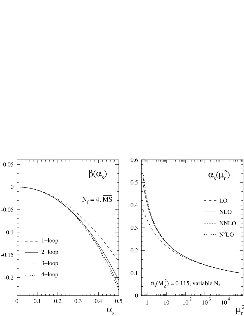
Figure 5: Left: The perturbative expansion of the QCD $\beta$-function up to order $\alpha_{s}^{5}$, for four flavours in the $\overline{\mbox{MS}}$ renormalization scheme. Right: Illustration of the resulting scale dependence of $\alpha_{s}$, using a variable $N_{f}$ as detailed in the text. $\mu_{r}^{2}$ is given in GeV².

For illustrations of the scale dependence of the parton densities and structure functions, initial distributions have to be chosen at some reference scales, in the following denoted by $\mu_{f,0}^{2}$ and $Q_{0}^{2}$, respectively, in Eqs. (2.8) and (2.15). We will employ the function

$$f\,=\,x^{0.5}(1-x)^{3}$$ (5.1)

for all six quantities

$$f\,=\,xq_{\rm NS}^{\pm}(x,\mu_{f,0}^{2})\,,\>F_{2,\rm NS}^{\pm}(x,Q_{0}^{2})\,\>\>\mbox{ and }\>xF_{3,\rm NS}^{\pm}(x,Q_{0}^{2})\>\>.$$ (5.2)

Eq. (5.1) represents a simple model shape which incorporates the most important features of non-singlet $x$-distributions of nucleons. The same input is used in all cases, as this allows for a direct comparison of the effects of the various kernels in Eqs. (2.10) and (2.16). The overall normalization of $f$ is irrelevant for the logarithmic derivatives considered below. Our initial scales are specified via

$$\alpha_{s}(\mu_{r}^{2}\!=\!\mu_{f,0}^{2})\,=\,\alpha_{s}(\mu_{r}^{2}\!=\!Q_{0}^{2})\,=\,0.2\>\>,$$ (5.3)

irrespective of the order of the expansion. For $\alpha_{s}(M_{Z}^{2})=0.114\ldots 0.120$ this choice corresponds to $\mu_{f,0}^{2}=Q_{0}^{2}\,\simeq\,25\ldots 50$ GeV², a $Q^{2}$-region typical for fixed-target DIS. If not explicitly indicated otherwise, the results will be given for $N_{f}=4$ massless flavours.

Figure 6: The perturbative expansion of the scale derivative, $\dot{q}_{\rm NS}^{\,+}\equiv d\ln q_{\rm NS}^{\,+}/d\ln\mu_{f}^{2}$, for a non-singlet ‘+’-combination of quark densities at $\mu_{r}=\mu_{f}$. The initial conditions are as specified in Eqs. (5.1)–(5.3). Here and in what follows the subscripts A and B indicate the approximations for the 3-loop splitting functions derived in the previous section.

The evolution of $q_{\rm NS}^{\,+}(x,\mu_{f}^{2})$ is illustrated in Fig. 6 for the standard choice $\mu_{r}=\mu_{f}$ of the renormalization scale. In this case the perturbative expansion appears to be very well convergent: Except for the region around $x\simeq 0.07$ where the scale derivative is very small, the NNLO corrections for $\dot{q}_{\rm NS}^{\,+}\equiv d\ln q_{\rm NS}^{\,+}/d\ln\mu_{f}^{2}$ are as small as about 2%, while the NLO contributions typically amount to $10\ldots 20\%$. The residual uncertainty of the 3-loop splitting functions of Sect. 4 leads to a noticeable effect only for $x\raisebox{-1.9919pt}{$\>\stackrel{{\scriptstyle<}}{{{\scriptstyle\sim}}}\>$}0.02$, and even at $x\simeq 10^{-3}$ this effect does not exceed $\pm 2\%$ with respect to the central result $\frac{1}{2}({\rm NNLO}_{A}+{\rm NNLO}_{B})$ not shown in the figure. Over the full $x$-range the NNLO corrections are comparable to the dependence on the number of active flavours: If $N_{f}$ is increased (decreased) to $N_{f}=5$ ($N_{f}=3$), $\dot{q}_{\rm NS}^{\,+}$ is decreased (increased) by about 2%, respectively.

Figure 7: The dependence of the NLO and NNLO predictions for $d\ln q_{\rm NS}^{\,+}/d\ln\mu_{f}^{2}$ on the renormalization scale $\mu_{r}$ for six typical values of $x$.

Another way to assess the reliability of perturbative calculations is to investigate the stability of the results under variations of the renormalization scale $\mu_{r}$. In Fig. 7 the consequences of varying $\mu_{r}$ over the rather wide range $\frac{1}{8}\mu_{f}^{2}\leq\mu_{r}^{2}\leq 8\mu_{f}^{2}$ are displayed for six representative values of $x$. The relative scale uncertainties of the average results, estimated by

$$\Delta\dot{q}_{\rm NS}^{\,+}\,\equiv\,\frac{\max\,[\dot{q}_{\rm NS}^{\,+}(x,\mu_{r}^{2}=\frac{1}{4}\mu_{f}^{2}\ldots 4\mu_{f}^{2})]-\min\,[\dot{q}_{\rm NS}^{\,+}(x,\mu_{r}^{2}=\frac{1}{4}\mu_{f}^{2}\ldots 4\mu_{f}^{2})]}{2\,|\,{\rm average}\,[\dot{q}_{\rm NS}^{\,+}(x,\mu_{r}^{2}=\frac{1}{4}\mu_{f}^{2}\ldots 4\mu_{f}^{2})]\,|}$$ (5.4)

are shown in the left part of Fig. 8. Also this estimate leads to about 2% for the NNLO uncertainty, an improvement by more than a factor of three with respect to the corresponding NLO result. Even as low as $x\simeq 10^{-3}$ the NNLO calculation, despite its approximation uncertainty increasing towards small $x$, is superior to the NLO.

Finally the evolution of ‘$-$’-combinations $q_{\rm NS}^{\,-}$ is illustrated in the right part of Fig. 8. For $x>0.1$ the difference to the ‘+’-case discussed so far is negligible at NLO as well as at NNLO. At small $x$ the NLO predictions differ by up to 2%. As expected from the discussion in Sect. 4, the residual uncertainty of the NNLO result is considerably less pronounced at small $x$ in the ‘$-$’-case, but somewhat larger for $0.01\raisebox{-1.9919pt}{$\>\stackrel{{\scriptstyle<}}{{{\scriptstyle\sim}}}\>$}x\raisebox{-1.9919pt}{$\>\stackrel{{\scriptstyle<}}{{{\scriptstyle\sim}}}\>$}0.1$.

Figure 8: Left: The renormalization scale uncertainty of the NLO and NNLO predictions for the scale derivative of $q_{\rm NS}^{+}$, as obtained from the quantity $\Delta\dot{q}_{\rm NS}^{\,+}$ defined in Eq. (5.4). Right: The NNLO effects on the evolution of $q_{\rm NS}^{\,-}$ for the standard scale choice $\mu_{r}=\mu_{f}$, together with a comparison of the NLO partonic NS⁺ and NS^- evolutions.

We now turn to the evolution of the non-singlet structure functions. The physical scale derivative $\dot{F}_{2,\rm NS}^{\,+}\equiv d\ln F_{2,\rm NS}^{\,+}/d\ln Q^{2}$ is shown in the left part of Fig. 9 for $\mu_{r}=Q$. Besides the splitting functions $P_{\rm NS}^{(1,2)+}(x)$ the effect of which has been illustrated in Fig. 6, here also the coefficient functions $c_{2,\rm NS}^{(1)}(x)$ and $c_{2,\rm NS}^{(2)+}(x)$ enter the NLO and NNLO evolution kernels as detailed in Eq. (2.16). These additional terms considerably increase the $Q^{2}$-dependence at large $x$, as can be seen by comparing Fig. 6 and Fig. 9. E.g., the NNLO corrections rise from 4% at $x=0.5$ to about 7, 11 and 21% at $x=0.65$, 0.8 and $x=0.95$, respectively. The corresponding NLO contributions amount to 24, 30, 37 and 51% of the LO results. Unlike for the parton densities, the NNLO corrections to the structure functions are larger than the $N_{f}$-dependence at large $x$: If $N_{f}$ is increased (decreased) to $N_{f}=5$ ($N_{f}=3$), $\dot{F}_{2\rm NS}^{\,+}$ is decreased (increased) between 3.5% and 7% for $0.5\leq x\leq 0.95$, respectively.

The worse convergence of the expansion at large $x$ is due to the large soft-gluon contributions $[\ln^{k}(1\!-\!x)/(1\!-\!x)]_{+}$, $k=1,\ldots,2l\!-\!1$, to $c_{2,\rm NS}^{(l)\pm}(x)$ which are conjectured to be absent [24] in the $\overline{\mbox{MS}}$ splitting functions $P_{\rm NS}^{(l)+}(x)$. Consequently, as shown in the right part of Fig. 9, keeping only the coefficient-function contributions in the $O(\alpha_{s}^{3})$ term of Eq. (2.16) yields a very good approximation at large $x$. In fact $P_{\rm NS}^{(2)+}$ contributes less than 2% to the total NNLO derivative $\dot{F}_{2,\rm NS}^{\,+}$ at $x>0.2$. The residual uncertainty of $P_{\rm NS}^{(2)+}$, given by the difference NNLO_A – NNLO_B, is thus completely negligible in this region.

Figure 9: The perturbative expansion of the scale derivative, $\dot{F}_{2,\rm NS}^{\,+}\equiv d\ln F_{2,\rm NS}^{\,+}/d\ln Q^{2}$, for a non-singlet structure function at $\mu_{r}=\mu_{f}$. The initial conditions are as specified in Eqs. (5.1)–(5.3), the leading-order curve is identical to that of Fig. 6. Also shown (right part) is the effect of omitting the contribution from the 3-loop splitting function $P_{\rm NS}^{(2)+}$.

The dependence of $\dot{F}_{2,\rm NS}^{\,+}$ on the renormalization scale $\mu_{r}$ is presented in Fig. 10 and Fig. 11 (left part), analogously to the partonic case (see Eq. (5.4)) in Figs. 7 and 8 using

$$\Delta\dot{F}_{2,\rm NS}^{\,+}\,\equiv\,\frac{\max\,[\dot{F}_{2,\rm NS}^{\,+}(x,\mu_{r}^{2}=\frac{1}{4}Q^{2}\ldots 4Q^{2})]-\min\,[\dot{F}_{2,\rm NS}^{\,+}(x,\mu_{r}^{2}=\frac{1}{4}Q^{2}\ldots 4Q^{2})]}{2\,|\,{\rm average}\,[\dot{F}_{2,\rm NS}^{\,+}(x,\mu_{r}^{2}=\frac{1}{4}Q^{2}\ldots 4Q^{2})]\,|}\>\>.$$ (5.5)

The slower large-$x$ convergence of the $\alpha_{s}$ series for $\dot{F}_{2,\rm NS}^{\,+}$ is obvious from these results as well, e.g., no extremum close to $\mu_{r}=Q$ is obtained for $x=0.8$. The NNLO uncertainties as estimated using Eq. (5.5) read 3%, 4.5% and 7% for $x=0.5$, 0.65 and 0.8. The corresponding NLO results are 8.5%, 10.5% and 12%, respectively. The accuracy of the $Q^{2}$-slope predictions is thus improved by a factor $2\ldots 3$ except for very large $x$.

Figure 10: The dependence of the NLO and NNLO predictions for $d\ln F_{2,\rm NS}^{\,+}/d\ln Q^{2}$ on the renormalization scale $\mu_{r}$ for six typical values of $x$.

Figure 11: Left: The $\mu_{r}$-uncertainty of the scale derivative of $F_{2,\rm NS}^{+}$, as estimated by $\Delta\dot{F}_{2,\rm NS}^{\,+}$ defined in Eq. (5.5). Note that the absolute values of $\dot{F}_{2,\rm NS}^{\,+}$ are very small for $0.05<x<0.15$. Right: The NNLO effects on the evolution of $F_{2,\rm NS}^{\,-}$ for $\mu_{r}=\mu_{f}$, together with a comparison of the NS⁺ and NS^- evolutions for $F_{2,\rm NS}$ at NLO.

Figure 12: The scale derivative $\dot{F}_{3,\rm NS}^{\,-}\equiv d\ln F_{3,\rm NS}^{\,-}/d\ln Q^{2}$ at $\mu_{r}=\mu_{f}$. The initial conditions are as given in Eqs. (5.1)–(5.3), the leading-order curve is the same as in Figs. 6 and 9. Also shown (right part) is the ratio of $\dot{F}_{3,\rm NS}^{\,-}$ to the corresponding result for $F_{2,\rm NS}^{\,+}$.

As for the parton densities shown in Fig. 8, the evolution of $F_{2,\rm NS}^{\,-}$ illustrated in the right part of Fig. 11 is indistinguishable from that of $F_{2,\rm NS}^{\,+}$ at $x>0.1$, while being better constrained at NNLO at very small $x$. For $x\simeq 10^{-3}$, the $2.5\%\ldots 3.5\%$ positive effect of $P_{\rm NS}^{(2)-}$ in Fig. 8 is overcompensated by the coefficient-function contributions. This effect also occurs for $\dot{F}_{2,\rm NS}^{\,+}$ not displayed at small $x$. In both cases the NLO corrections are smaller than for $\dot{q}_{\rm NS}^{\pm}$, resulting in a better small-$x$ NLO renormalization-scale stability of $\dot{F}_{2,\rm NS}^{\,\pm}$ as can be seen by comparing the left parts of Fig. 11 and Fig. 8.

The scaling violations of $F_{3,\rm NS}^{\,-}$ are presented in Fig. 12 for the medium- to large-$x$ region. Since the soft-gluon terms $[\ln^{k}(1\!-\!x)/(1\!-\!x)]_{+}$ are identical in $c_{2,\rm NS}^{\pm(l)}$ and $c_{3,\rm NS}^{\pm(l)}$, the results for $\dot{F}_{3,\rm NS}$ and $\dot{F}_{2,\rm NS}$ agree (for identical initial distributions as assumed here) as $x\!\rightarrow\!1$. However, the different regular terms lead to noticeable differences already at medium $x$, reaching 5% and 10% at $x\simeq 0.4$ and 0.3, respectively. At small $x$ the corrections are considerably larger for $\dot{F}_{3,\rm NS}$ than for $\dot{F}_{2,\rm NS}$, resulting in scale uncertainties of about 10% at NLO and 4% at NNLO for $10^{-3}\raisebox{-1.9919pt}{$\>\stackrel{{\scriptstyle<}}{{{\scriptstyle\sim}}}\>$}x\raisebox{-1.9919pt}{$\>\stackrel{{\scriptstyle<}}{{{\scriptstyle\sim}}}\>$}10^{-2}$ for the former quantity.

Finally we turn to the determination of $\alpha_{s}$ from scaling violations of non-singlet structure functions. Here we address the uncertainties $\Delta\alpha_{s}$ which arise from the truncation of the perturbation series, confining ourselves to the region $x\raisebox{-1.9919pt}{$\>\stackrel{{\scriptstyle>}}{{{\scriptstyle\sim}}}\>$}0.25$ of considerable negative scale derivatives $\dot{F}_{2,NS}$. In this region the results for $\dot{F}_{3,\rm NS}$ are rather similar to those for $\dot{F}_{2,\rm NS}$ and need not to be considered separately. We also disregard the negligible large-$x$ differences between the scaling violations of $F_{2,\rm NS}^{\,+}$ and $F_{2,\rm NS}^{\,-}$ and between the NNLO_A and NNLO_B calculations. Our procedure for estimating $\Delta\alpha_{s}$ is as follows: For each $x$ we determine those scales $\mu_{r,\rm min}$ and $\mu_{r,\rm max}$ which led to the minimal and maximal NLO and NNLO results for $|\dot{F}_{2,\rm NS}|$ used in Eq. (5.5). The value of $\alpha_{s}(Q_{0}^{2})$ is then adjusted to obtain, at these values of $x$ and $\mu_{r}$, the same results for $\dot{F}_{2,\rm NS}$ as found for $\mu_{r}=Q_{0}$ and $\alpha_{s}(Q_{0}^{2})=0.2$ (Fig. 9, left part). The latter standard-scale results thus play the role of the experimental results for $\dot{F}_{2,\rm NS}$ in determinations of $\Delta\alpha_{s}$ in data fits.

The resulting upper and lower limits for $\alpha_{s}(Q_{0}^{2})$ are shown in the left part in Fig. 13. Due to the increase of the higher-order corrections towards large $x$ discussed above, the uncertainty $\Delta\alpha_{s}$ rises with increasing $x$. As available experimental DIS results are restricted to $x\leq 0.85$ [2], we choose a value $x\simeq 0.55$ for estimating the $x$-averaged uncertainties given by the differences to the reference result $\alpha_{s}(Q_{0}^{2})=0.2$. This procedure yields

$$\Delta\alpha_{s}(Q_{0}^{2}\simeq 25\ldots 50\mbox{ GeV}^{2})_{\rm NLO}\>\>\>={\footnotesize\begin{array}[]{c}+\,0.020\\ -\,0.012\end{array}}\>\>,$$ (5.6)

$$\Delta\alpha_{s}(Q_{0}^{2}\simeq 25\ldots 50\mbox{ GeV}^{2})_{\rm NNLO}\,={\footnotesize\begin{array}[]{c}+\,0.008\\ -\,0.004\end{array}}\>\>.$$ (5.7)

Often results and uncertainties for $\alpha_{s}$ from different processes and observables are compared after evolution to a common reference scale, conventionally chosen as the Z-boson mass $M_{Z}$. Adopting $Q_{0}^{2}=30$ GeV² (and $N_{f}=5$ for $Q_{0}\leq\mu_{r}\leq M_{Z}$) for definiteness, one obtains the error bands displayed in the right part of Fig. 13 and

$$\Delta\alpha_{s}(M_{Z}^{2})_{\rm NLO}\>={\footnotesize\begin{array}[]{l}+\>0.006\\ -\>0.004\end{array}}\>,\>\>\>\>\Delta\alpha_{s}(M_{Z}^{2})_{\rm NNLO}\>={\footnotesize\begin{array}[]{l}+\>0.0025\\ -\>0.0015\end{array}}\>\>.$$ (5.8)

As expected from our previous discussions below Eq. (5.5), the NNLO calculation reduces the theoretical uncertainty under consideration by a factor of about 2.5.

In a data analysis, also the NLO and NNLO central values for $\alpha_{s}(Q_{0}^{2})$ will be different, since the NNLO scaling violations are stronger over most of the large-$x$ region as shown in Fig. 9. A simple estimate analogous to that for $\Delta\alpha_{s}$ yields

$$\alpha_{s}(M_{Z}^{2})_{\rm NNLO}-\alpha_{s}(M_{Z}^{2})_{\rm NLO}\>\simeq\>-\,0.002\>\>.$$ (5.9)

Due to the strong $x$-dependence of the NNLO/NLO ratio, this estimate is less reliable than Eq. (5.8), its uncertainty amounts to about $\pm 0.001$. Nevertheless it is interesting to note that Eq. (5.9) agrees with the findings of ref. [13] from analyses of data on $F_{3}$. The 3-loop splitting function $P_{\rm NS}^{(2)}$ contribute only about $-0.0007$ to the shift (5.9) of the NNLO result.

Figure 13: Right: The $x$-dependent theoretical uncertainty of the determination of $\alpha_{s}$ from the scale derivative of $F_{2,\rm NS}$ at $Q_{0}^{2}=25\ldots 50$ GeV², estimated by the $\mu_{r}$-variation $\frac{1}{4}Q_{0}^{2}\leq\mu_{r}^{2}\leq 4Q_{0}^{2}$. The scales leading to a maximal (minimal) $|\dot{F}_{2\rm NS}|$ are denoted by $\mu_{r,\rm max}$ ($\mu_{r,\rm min}$). Left: The resulting error band for $\alpha_{s}(M_{Z}^{2})$ using $Q_{0}^{2}=30$ GeV² and $N_{f}=5$.

6 Summary

We have investigated the effect of the NNLO perturbative QCD corrections on the scale dependence of flavour non-singlet quark densities and structure functions. For this purpose, and for application in further analyses, we have derived compact parametrizations of the corresponding three-loop splitting functions $P_{\rm NS}^{(2)\pm}$ and the two-loop coefficient functions $c_{a,\rm NS}^{(2)\pm}$, $a=2,3,L$. The latter quantities are exactly known [5, 6, 7]; their analytic $x$-dependent expressions are however rather cumbersome and not readily transformed to moment space [21]. Our parametrizations of $c_{a,\rm NS}^{(2)\pm}(x)$ and their Mellin transforms thus provide a convenient technical tool. They agree to the exact results up to a few permille or less over the full $x$-range, thus introducing a negligible error of well below 0.1% after insertion into the perturbative expansions.

As only partial results are presently available for the three-loop splitting functions [8, 15, 18], our parametrizations of $P_{\rm NS}^{(2)\pm}(x)$ serve the additional purpose of providing quantitative estimates of their $x$-dependent residual uncertainties. The function $P_{\rm NS}^{(2)+}(x)$, relevant to the evolution of flavour asymmetries like $u+\bar{u}-[d+\bar{d}]$, is well constrained at large $x$ by the lowest even-integer moments of refs. [8], the spread reaching about $\pm 7\%$ at $x\simeq 0.3$. On the other hand $P_{\rm NS}^{(2)+}(x)$ is very weakly constrained for $x\raisebox{-1.9919pt}{$\>\stackrel{{\scriptstyle<}}{{{\scriptstyle\sim}}}\>$}10^{-2}$ so far, despite the fact that the leading small-$x$ term is known [18]. The quantity $P_{\rm NS}^{(2)-}(x)$, entering the evolution of the quark-antiquark differences, is somewhat better (worse) constrained at small $x$ (medium $x$), respectively, than $P_{\rm NS}^{(2)+}(x)$. As the splitting functions enter parton densities and structure functions only via convolutions with smooth non-perturbative initial distributions, these ‘bare’ uncertainties are very much reduced for physical quantities over the whole $x$-range. E.g., the spread of $P_{\rm NS}^{(2)+}$ leads to effects of less than $\pm 0.2\%$ at $x\raisebox{-1.9919pt}{$\>\stackrel{{\scriptstyle>}}{{{\scriptstyle\sim}}}\>$}0.2$ after convolution with typical nucleonic input shapes. In this region the present uncertainties of $P_{\rm NS}^{(2)\pm}$ are thus rendered absolutely negligible, leading to effects even below 0.01% after insertion into the perturbation series. Their impact becomes significant only for $x\raisebox{-1.9919pt}{$\>\stackrel{{\scriptstyle<}}{{{\scriptstyle\sim}}}\>$}10^{-2}$, without seriously impairing the NNLO calculations even down to $x\simeq 10^{-3}$.

The perturbative expansion for the scale dependence $d\ln q_{\rm NS}^{\,\pm}(x,\mu_{f}^{2})/d\ln\mu_{f}^{2}$ of the non-singlet combinations of quark densities appears to be very well convergent. For $\alpha_{s}=0.2$, corresponding to scales of about 25–50 GeV², the NNLO effects of $P_{\rm NS}^{(2)\pm}$ are on the level of 2% rather uniformly in $x$. This result is to be compared to the NLO corrections which amount to 10–20%. Also the variation of the renormalization scale leads to effects of about $\pm 2\%$ at NNLO. Corrections of this size are comparable to the dependence of the predictions on the number of quark flavours, rendering a proper treatment of charm effects [27] rather important even for large-$x$ non-singlet quantities.

Especially at $x>0.5$, the higher-order corrections are much larger for the scale derivative $d\ln F_{a,\rm NS}^{\,\pm}(x,Q^{2})/d\ln Q^{2}$, $a=2,3$, of the non-singlet structure functions. This enhancement is an effect of the coefficient functions containing large $[\ln^{k}(1\!-\!x)/(1\!-\!x)]_{+}$ soft-gluon terms, which are conjectured to be absent in the $\overline{\mbox{MS}}$ splitting functions [24]. E.g., the NLO and NNLO effects reach about 37% and 11% of the respective lower-order results at $x=0.8$ for $\alpha_{s}=0.2$ and four flavours. The NNLO calculations thus represent a distinct improvement, reducing also the renormalization-scale dependence of the predictions by a factor of two to three, e.g., to about $\pm 7\%$ at $x=0.8$. Accordingly the inclusion of the NNLO corrections into fits of data on non-singlet scaling violations is expected to yield, besides a slight lowering of the central values for $\alpha_{s}(M_{Z}^{2})$ by roughly 0.002, a considerable reduction of the (so far dominant) theoretical error due to the truncation of the perturbation series,

$$\Delta\alpha_{s}(M_{Z}^{2})_{\rm NNLO}\>={\footnotesize\left.\begin{array}[]{l}+\>0.0025\!\\ -\>0.0015\end{array}\right|}_{\,{\mbox{\small$\mu$}}_{\mbox{\scriptsize$r$}}}\>\>.$$

These estimates are compatible with the results of the fits of $F_{3,\rm NS}$-data performed in ref. [13], where an alternative, integer-moment based approach to the calculation of the scaling violations has been pursued.

Fortran subroutines of our parametrizations of $c_{a,\rm NS}^{(2)\pm}(x)$, $a=2,3,L$, and $P_{\rm NS}^{(2)\pm}(x)$ can by obtained via email to neerven@lorentz.leidenuniv.nl or avogt@lorentz.leidenuniv.nl.

Appendix: Third-order quantities in Mellin-$N$ space

The Mellin transforms of the approximate NNLO expressions of Sect. 3 and Sect. 4 are given in terms of the integer-$N$ sums $S_{l}(N)$ and their analytic continuations

$$S_{l}\equiv S_{l}(N)=\sum_{k=1}^{N}\frac{1}{k^{l}}=\zeta(l)-\frac{(-1)^{l}}{(l-1)!}\,\psi^{(l-1)}(N\!+\!1)\>\>.$$ (A.1)

Here $\zeta(1)$ stands for the Euler–Mascheroni constant, and $\zeta(l\!>\!1)$ for Riemann’s $\zeta$-function. The $l\,$th logarithmic derivative $\psi^{(l-1)}$ of the $\Gamma$-function can be readily evaluated using the asymptotic expansion for ${\rm Re}\,N>10$ together with the functional equation.

Due to the simplicity of our parametrizations for the three-loop splitting functions, only the most simple Mellin transforms occur for these quantities. Therefore we are able to dispense with details here. The Mellin-$N$ dependence of the exactly known $N_{F}^{2}$-piece can be found in ref. [15].

The moments the non-singlet ‘+’-coefficient function (3.2) entering $F_{2}^{\,{\rm e.m.}}$ are given by

$$c_{2,{\rm NS}}^{(2)+}(N)\! =\! \mbox{}+3.55555\,\Big{(}6\,S_{4}+8\,S_{3}S_{1}+3\,S_{2}^{2}+6\,S_{2}S_{1}^{2}+S_{1}^{4}\Big{)}$$

$$\mbox{}+20.4444\,\Big{(}2\,S_{3}+3\,S_{2}S_{1}+S_{1}^{3}\Big{)}-15.5525\,\Big{(}S_{2}+S_{1}^{2}\Big{)}-188.64\,S_{1}$$

$$\mbox{}+\frac{165.356}{N}S_{3}-\bigg{(}\frac{15.38}{N^{2}}-\frac{9.7467}{N}\bigg{)}S_{2}+\frac{358.503}{N}S_{2}S_{1}+\frac{2.9678}{N}S_{1}^{3}$$

$$\mbox{}+\bigg{(}\frac{174.8}{N^{2}}+\frac{9.7467}{N}\bigg{)}S_{1}^{2}-\bigg{(}\frac{190.18}{N^{3}}-\frac{116.734}{N}\bigg{)}S_{1}$$

$$\mbox{}+\frac{17.01}{N^{4}}-\frac{34.16}{N^{3}}+\frac{306.849}{N^{2}}-\frac{72.5824}{N}-\frac{1008}{N+1}-338.044$$

$$\mbox{}+N_{f}\>\bigg{\{}-0.59259\,\Big{(}2\,S_{3}+3\,S_{2}S_{1}+S_{1}^{3}\Big{)}-4.2963\,\Big{(}S_{2}+S_{1}^{2}\Big{)}-6.3489\,S_{1}$$

$$\mbox{}-\frac{6.072}{N}S_{3}-\bigg{(}\frac{6.072}{N^{2}}-\frac{18.0408}{N}\bigg{)}S_{2}-\bigg{(}\frac{6.072}{N^{3}}-\frac{17.97}{N^{2}}+\frac{14.3574}{N}\bigg{)}S_{1}$$

$$\mbox{}+\frac{0.07078}{N}S_{1}^{2}+\frac{4.488}{N^{3}}+\frac{4.21808}{N^{2}}-\frac{21.6028}{N}-\frac{37.91}{N+1}+46.8406\bigg{\}}\>\>.$$

For the charged current ‘$-$’-combination the third to fifth line of this result are, according to Eq. (3.3), replaced by

$$\mbox{}+\frac{229.916}{N}S_{3}+\bigg{(}\frac{31.58}{N^{2}}+\frac{9.7467}{N}\bigg{)}S_{2}+\frac{393.703}{N}S_{2}S_{1}+\frac{2.9678}{N}S_{1}^{3}$$

$$\mbox{}+\bigg{(}\frac{192.4}{N^{2}}+\frac{9.7467}{N}\bigg{)}S_{1}^{2}-\bigg{(}\frac{160.82}{N^{3}}-\frac{61.1321}{N}\bigg{)}S_{1}$$ (A.3)

$$\mbox{}+\frac{22.488}{N^{4}}-\frac{39.12}{N^{3}}+\frac{265.774}{N^{2}}-\frac{164.777}{N}-\frac{1010}{N+1}-337.992\>\>.$$

The first two lines and the sixth line of Eq. (A.2) stem from the universal +-distribution parts of Eq. (3.2). They are exact up to a truncation of the numerical factors [6].

The corresponding $N$-space results for the coefficient functions (3.4) and (3.5) for $F_{L}$ read

$$c_{L,{\rm NS}}^{(2)+}(N)\! =\! \mbox{}-\frac{136.88}{N}S_{2}+\frac{13.62}{N}S_{1}^{2}+\bigg{(}\frac{55.79}{N}-\frac{150.5}{N^{2}}\bigg{)}S_{1}-\frac{0.062}{N^{3}}$$

$$\mbox{}+\frac{14.85}{N^{2}}+\frac{207.153}{N}+\frac{53.12}{(N+1)^{3}}+\frac{97.48}{N+1}-0.164$$

$$\mbox{}+N_{f}\>\frac{16}{27}\>\bigg{\{}-\frac{6}{N+1}S_{1}+\frac{6}{N}+\frac{6}{(N+1)^{2}}-\frac{25}{N+1}\bigg{\}}$$

and

$$c_{L,{\rm NS}}^{(2)-}(N)\! =\! \mbox{}-\frac{128.4}{N}S_{2}+\frac{13.30}{N}S_{1}^{2}+\bigg{(}\frac{59.12}{N}-\frac{141.7}{N^{2}}\bigg{)}S_{1}-\frac{0.086}{N^{3}}$$

$$\mbox{}+\frac{22.21}{N^{2}}+\frac{180.818}{N}+\frac{46.58}{(N+1)^{3}}+\frac{100.8}{N+1}-0.150$$

$$\mbox{}+N_{f}\>\frac{16}{27}\>\bigg{\{}-\frac{6}{N+1}S_{1}+\frac{6}{N}+\frac{6}{(N+1)^{2}}-\frac{25}{N+1}\bigg{\}}\>\>.$$

Here the $N_{f}$ parts represent an exact result [5].

The ‘$-$’-coefficient function (3.6) for $F_{3}$, occurring in the $\nu\!+\!\bar{\nu}$ sum, leads to

$$c_{3,\rm NS}^{(2)-}(N)\! =\! \mbox{}+3.55555\,\Big{(}6\,S_{4}+8\,S_{3}S_{1}+3\,S_{2}^{2}+6\,S_{1}^{2}S_{2}+S_{1}^{4}\Big{)}$$

$$\mbox{}+20.4444\,\Big{(}2\,S_{3}+3\,S_{2}S_{1}+S_{1}^{3}\Big{)}-15.5525\,\Big{(}S_{2}+S_{1}^{2}\Big{)}-188.64\,S_{1}$$

$$\mbox{}+\frac{297.756}{N}S_{3}+\bigg{(}\frac{147.9}{N^{2}}+\frac{33.2767}{N}\bigg{)}S_{2}+\frac{298.733}{N}S_{2}S_{1}+\frac{0.9778}{N}S_{1}^{3}$$

$$\mbox{}+\bigg{(}\frac{147.9}{N^{2}}+\frac{33.2767}{N}\bigg{)}S_{1}^{2}-\frac{45.8683}{N}S_{1}$$

$$\mbox{}+\frac{23.532}{N^{4}}-\frac{66.62}{N^{3}}+\frac{67.6}{N^{2}}-\frac{373.029}{N}-\frac{576.8}{N+1}-338.625$$

$$\mbox{}+N_{f}\>\bigg{\{}-0.59259\,\Big{(}2\,S_{3}+3\,S_{2}S_{1}+S_{1}^{3}\Big{)}-4.2963\,\Big{(}S_{2}+S_{1}^{2}\Big{)}-6.3489\,S_{1}$$

$$\mbox{}-\frac{0.042}{N}\Big{(}2\,S_{3}+3\,S_{2}S_{1}+S_{1}^{3}\Big{)}+\frac{0.96978}{N}S_{1}^{2}+\bigg{(}\frac{9.684}{N^{2}}-\frac{16.4074}{N}\bigg{)}S_{1}$$

$$\mbox{}+\frac{10.6538}{N}S_{2}+\frac{4.414}{N^{3}}-\frac{8.683}{N^{2}}-\frac{15.9177}{N}-\frac{14.97}{N+1}+46.856\bigg{\}}\>\>.$$

For the ‘+’-combination of Eq. (3.7) entering $F_{3}^{\nu N}-F_{3}^{\bar{\nu}N}$ one has to replace the third to fifth line of the above result by

$$\mbox{}+\frac{186.816}{N}S_{3}+\bigg{(}\frac{92.43}{N^{2}}+\frac{33.2767}{N}\bigg{)}S_{2}+\frac{187.793}{N}S_{2}S_{1}+\frac{0.9778}{N}S_{1}^{3}$$

$$\mbox{}+\bigg{(}\frac{92.43}{N^{2}}+\frac{33.2767}{N}\bigg{)}S_{1}^{2}+\frac{123.121}{N}S_{1}$$ (A.7)

$$\mbox{}+\frac{18.294}{N^{4}}-\frac{60.28}{N^{3}}+\frac{79.14}{N^{2}}-\frac{276.473}{N}-\frac{467.2}{N+1}-338.681\>\>.$$

References

• [1] D.H. Coward et al., Phys. Rev. Lett. 20 (1968) 292;
E.D. Bloom et al., Phys. Rev. Lett. 23 (1969) 930;
H. Breitenbach et al., Phys. Rev. Lett. 23 (1969) 935
• [2] C. Caso et al., Particle Data Group, Eur. Phys. J. C3 (1998) 1, and references therein
• [3] W. Furmanski and R. Petronzio, Z. Phys. C11 (1982) 293, and references therein
• [4] O.V. Tarasov, A.A. Vladimirov, and A.Yu. Zharkov, Phys. Lett. B93 (1980) 429;
S.A. Larin and J.A.M. Vermaseren, Phys. Lett. B303 (1993) 334
• [5] J. Sanchez Guillen et al., Nucl. Phys. B353 (1991) 337
• [6] E.B. Zijlstra and W.L. van Neerven, Phys. Lett. B272 (1991) 127, ibid. B273 (1991) 476, ibid. B297 (1992) 377
• [7] E.B. Zijlstra and W.L. van Neerven, Nucl. Phys. B383 (1992) 525;
E.B. Zijlstra, thesis, Leiden University 1993
• [8] S.A. Larin, T. van Ritbergen, and J.A.M. Vermaseren, Nucl. Phys. B427 (1994) 41;
S.A. Larin, P. Nogueira, T. van Ritbergen, and J.A.M. Vermaseren, Nucl. Phys. B492 (1997) 338,
T. van Ritbergen, thesis, Amsterdam University 1996
• [9] R. Hamberg, W.L. van Neerven and T. Matsuura, Nucl. Phys. B359 (1991) 343;
R. Hamberg, thesis, Leiden University 1991;
W.L. van Neerven and E.B. Zijlstra, Nucl. Phys. B382 (1992) 11
• [10] A.D. Martin, R.G. Roberts and W.J. Stirling, Phys. Lett. B387 (1996) 419;
A.D. Martin, R.G. Roberts, W.J. Stirling and R.S. Thorne, Eur. Phys. J. C4 (1998) 463
• [11] H.L. Lai et al., CTEQ Collab., Phys. Rev. D55 (1997) 1280; Michigan State University preprint MSU-HEP-903100 (hep-ph/9903282)
• [12] M. Glück, E. Reya and A. Vogt, Z. Phys. C67 (1995) 433; Eur. Phys. J. C5 (1998) 461
• [13] A.L. Kataev, A.V. Kotikov, G. Parente and A.V. Sidorov, Phys. Lett. B388 (1996) 179; ibid. B417 (1998) 374;
A.L. Kataev, G. Parente, A.V. Sidorov, ICTP preprint IC/99/51 (hep-ph/9905310)
• [14] J. Santiago and F.J. Yndurain, Madrid University preprint FTUAM-99-8 (hep-ph/ 9904344)
• [15] J. A. Gracey, Phys. Lett. B322 (1994) 141
• [16] J.F. Bennett and J.A. Gracey, Nucl. Phys. B517 (1998) 241
• [17] S. Catani and F. Hautmann, Nucl. Phys. B427 (1994) 475
• [18] J. Bümlein and A. Vogt, Phys. Lett. B370 (1996) 149
• [19] J. Blümlein and A. Vogt, Phys. Rev. D58 (1998) 014020;
J. Blümlein, V. Ravindran, W.L. van Neerven and A. Vogt, Proceedings of DIS 98, Brussels, April 1998, eds. Gh. Coremans and R. Roosen (World Scientific 1998), p. 211 (hep-ph/9806368)
• [20] M. Diemoz, F. Ferroni, E. Longo and G. Martinelli, Z. Phys. C39 (1988) 21;
M. Glück, E. Reya and A. Vogt, Z. Phys. C48 (1990) 471;
Ch. Berger, D. Graudenz, M. Hampel and A. Vogt, Z. Phys. C70 (1996) 77
• [21] J. Blümlein and S. Kurth, DESY preprint 97-160 (hep-ph/9708388); Phys. Rev. D60 (1999) 014018
• [22] J. Kirschner and L.N. Lipatov, Nucl. Phys. B213 (1983) 122
• [23] G. Curci, W. Furmanski and R. Petronzio, Nucl. Phys. B175 (1980) 27
• [24] A. Gonzales-Arroyo, C. Lopez and F.J. Yndurain, Nucl. Phys. B126 (1979) 161
• [25] J. Blümlein, S. Riemersma and A. Vogt, Nucl. Phys. (Proc. Suppl.) 51C (1996) 30 (hep-ph/9608470)
• [26] T. van Ritbergen, J.A.M. Vermaseren and S.A. Larin, Phys. Lett. B400 (1997) 379
• [27] E. Laenen, S. Riemersma, J. Smith, W.L. van Neerven, Nucl. Phys. B392 (1993) 162;
M. Buza, Y. Matiounine, J. Smith and W.L. van Neerven, Eur. Phys. J. C1 (1998) 301, and references therein