Experimental Signatures of Fermiophobic Higgs bosons

Abstract

The most general Two Higgs Doublet Model potential without explicit $CP$ violation depends on 10 real independent parameters. Excluding spontaneous $CP$ violation results in two 7 parameter models. Although both models give rise to 5 scalar particles and 2 mixing angles, the resulting phenomenology of the scalar sectors is different.

If flavour changing neutral currents at tree level are to be avoided, one has, in both cases, four alternative ways of introducing the fermion couplings. In one of these models the mixing angle of the $CP$ even sector can be chosen in such a way that the fermion couplings to the lightest scalar Higgs boson vanishes. At the same time it is possible to suppress the fermion couplings to the charged and pseudo-scalar Higgs bosons by appropriately choosing the mixing angle of the $CP$ odd sector.

We investigate the phenomenology of both models in the fermiophobic limit and present the different branching ratios for the decays of the scalar particles. We use the present experimental results from the LEP collider to constrain the models.

PACS number(s): 12.60.Fr, 14.80.Cp

1 Introduction

The $SU(2)\times U(1)$ electroweak model describes our world at the presently attainable energies. Nevertheless, it is hard to hide the frustration about our ignorance on the mass generation mechanism. The spontaneous symmetry breaking mechanism requires a single doublet of complex scalar fields. But does nature follow this minimal version or does it require a multi-Higgs sector?

The current search at LEP already constrains the mass of a neutral Higgs boson with a standard model like coupling to the fermions to $m_{H}>91.0\ GeV$ [1]. Nevertheless some multi-Higgs models allow the existence of Higgs particles with a vanishing coupling to the fermions. In this paper we investigate all type I $CP$ conserving Two Higgs Doublets models (2HDM) with such a vanishing coupling to the fermions. We will predict the experimental signatures of these particles.

Our paper is organized as follows: first we review the different 2HDM potentials to fix our notation. Thereafter we try to restrict the physical parameters of the potentials with theoretical constraints. Then we will discuss the signature of the different particles and show all characteristic branching ratios. Finally we constrain the models’ parameters using the current experimental data.

2 The potentials

The minimal version of the standard model which allows spontaneous symmetry breaking requires one scalar doublet of complex fields. To assure the renormalizability of the theory, the most general potential is

$$V=-\mu^{2}\phi^{\dagger}\phi+\lambda\left(\phi^{\dagger}\phi\right)^{2}\enskip,$$ (1)

where $\mu$ and $\lambda$ are real independent parameters. The mass eigenstate is a $C$-even scalar particle, the Higgs boson.

The simplest generalization of the potential amounts to the introduction of a second doublet of complex fields. The most general renormalizable potential invariant under $SU(2)\times U(1)$ has fourteen independent real parameters. The number of predicted particles grows from one to five. If one imposes that the potential is invariant under charge conjugation $C$, the number of parameters is reduced to ten. Defining $x_{1}=\phi_{1}^{\dagger}\phi_{1}$, $x_{2}=\phi_{2}^{\dagger}\phi_{2}$, $x_{3}=\Re\{\phi_{1}^{\dagger}\phi_{2}\}$ and $x_{4}=\Im\{\phi_{1}^{\dagger}\phi_{2}\}$ it can be shown [2] that the most general 2HDM potential without explicit $C$ violation is:

$$V=-\mu_{1}^{2}x_{1}-\mu_{2}^{2}x_{2}-\mu_{12}^{2}x_{3}+\lambda_{1}x_{1}^{2}+\lambda_{2}x_{2}^{2}+\lambda_{3}x_{3}^{2}+\lambda_{4}x_{4}^{2}+\lambda_{5}x_{1}x_{2}+\lambda_{6}x_{1}x_{3}+\lambda_{7}x_{2}x_{3}\enskip,$$ (2)

where $\mu_{i}$ and $\lambda_{i}$ are real independent parameters. The number of parameters can be further reduced and there are two ways to accomplish it. First, the potential can be made invariant under the $Z_{2}$ transformation $\phi_{1}\rightarrow\phi_{1}$ and $\phi_{2}\rightarrow-\phi_{2}$. The resulting potential, which we call $V_{A}$, is

$$V_{A}=-\mu_{1}^{2}x_{1}-\mu_{2}^{2}x_{2}+\lambda_{1}x_{1}^{2}+\lambda_{2}x_{2}^{2}+\lambda_{3}x_{3}^{2}+\lambda_{4}x_{4}^{2}+\lambda_{5}x_{1}x_{2}\enskip.$$ (3)

If we allow a soft breaking term $-\mu_{12}^{2}x_{3}$ in $V_{A}$, we end up with a model with spontaneous $CP$-violation [3].

Second, it is possible to make the potential invariant under the global $U(1)$ transformation $\phi_{2}\rightarrow e^{i\theta}\phi_{2}$. The potential then reads:

$$V_{B}^{\prime}=-\mu_{1}^{2}x_{1}-\mu_{2}^{2}x_{2}+\lambda_{1}x_{1}^{2}+\lambda_{2}x_{2}^{2}+\lambda_{3}\left(x_{3}^{2}+x_{4}^{2}\right)+\lambda_{5}x_{1}x_{2}\enskip.$$ (4)

Since we have a global broken symmetry, there is an extra Goldstone boson in the theory. If we allow the same soft breaking term, $-\mu_{12}^{2}x_{3}$, in the potential, we end up with the scalar sector that has the same general structure as the scalar sector of the minimal super symmetric model (MSSM) [4]. We call this latter model $V_{B}$. Both $V_{A}$ and $V_{B}$ have seven degrees of freedom, the five particle masses and the two rotation angles ($\alpha,\beta$). The five particles can be grouped into 2 scalar ($h^{0}$,$H^{0}$), where the small letter denotes the less massive particle, 1 pseudo-scalar particle ($A^{0}$) and 2 charged particles ($H^{\pm}$). The main difference between the potentials is the self-couplings in the scalar sector.

3 The fermiophobic limit

Figure 1: Feynman diagram of the largest contribution to $h^{0}\rightarrow b\bar{b}$

Potentials $V_{A}$ and $V_{B}$ give rise to different self-couplings in the scalar sector. However, the scalar couplings to the gauge bosons and to the fermions are the same in both models. If flavour changing neutral currents (FCNC) induced by Higgs exchanges are to be avoided, one has four different ways to couple the scalars to the fermions. A technically natural way to achieve it is to extend the global symmetry to the Yukawa Lagrangian. This leads to two different ways of coupling the quarks to the scalars as well as two different ways of coupling the leptons to the scalars. The result is a total of four different models, usually denoted as model I, II, III and IV (cf. e.g. [6]).

In model I, the lightest $CP$-even scalar, $h^{0}$, couples to a fermion pair (quark or lepton) proportionally to $\cos\alpha$. Setting $\alpha=\pi/2$, $h^{0}$ becomes completely fermiophobic. However, $h^{0}$ can still decay to two fermion pair via $h^{0}\rightarrow W^{*}W(Z^{*}Z)\rightarrow 2\,\bar{f}f$ or $h^{0}\rightarrow W^{*}W^{*}(Z^{*}Z^{*})\rightarrow 2\,\bar{f}f$. We will include these decays in our analysis. It is worthwhile to point out that these processes occur near the $W(Z)$ threshold. Decays of $h^{0}$ to two fermions can also be induced by scalar and gauge boson loops (see e.g. fig. 1). In the 2HDM, the angle $\alpha$ has to be renormalized to render $h^{0}\rightarrow f\bar{f}$ finite. However, at $\alpha=\pi/2$, all one-loop decays $h^{0}\rightarrow f\bar{f}$ are finite. Thus we can impose the following condition for $\delta\alpha$: the renormalized one-loop decay width for $h^{0}\rightarrow f\bar{f}$ is equal to the finite unrenormalized decay width. This condition is equivalent to set $[\delta\alpha]_{\alpha=\pi/2}=0$. We have checked that this condition holds for all fermions. The only relevant one-loop decay is $h^{0}\rightarrow b\bar{b}$ due to a large contribution of the Feynman diagram shown in fig. 1 to the total decay width. Thus, on one hand, $h^{0}$ is not completely fermiophobic at $\alpha=\pi/2$, and on the other hand, all decays $h^{0}\rightarrow f\bar{f}$ but $h^{0}\rightarrow b\bar{b}$ are almost zero even at one-loop level.

The couplings of the $CP$-odd scalar, $A^{0}$, and of the charged scalar, $H^{\pm}$, are proportional to $\cot\beta$. If we want these particles to be fermiophobic as well, $\beta$ has to approach $\alpha$ ($\beta\rightarrow\alpha=\pi/2$). In this limit the coupling of $h^{0}$ to the vector bosons, which is proportional to the sine of $\delta\equiv\alpha-\beta$ tends to zero. Thus, $h^{0}$ is not only fermiophobic but also bosophobic and “ghostphobic” – $h^{0}$ always needs another scalar particle to be able to decay. The differences between potential $A$ and $B$ can be extremely important in this limit since $h^{0}$ will have different signatures in each model. In contrast, the heaviest $CP$-even scalar, $H^{0}$, acquires the Higgs standard model couplings to the fermions in this limit. We will relax the limit $\beta\approx\pi/2$ and analyze the decays as a function of $\delta$ and of the Higgs masses.

4 Theoretical mass limits

Although the parameters of the 2HDM’s are, in contrast to the MSSM, almost unconstrained, it is possible to derive some bounds on the masses of the scalar sector particles in the fermiophobic limit. We want to look for the allowed region in the $m_{h^{0}}$-$\beta$ plane so that the calculations do not leave the perturbative regime. Several methods of achieving theoretical bounds on these masses have been published [7]. Tree-level unitarity bounds have been derived in [8] and [9] for potential $A$. We use the bounds from [8]:

$$m_{h^{0}}\,\leq\,\sqrt{\frac{16\pi\sqrt{2}}{3\,G_{F}}\,\cos^{2}\beta\,-\,m_{H^{0}}^{2}\cot^{2}\beta}\enskip,$$ (5)

where $G_{F}=1.166\ GeV^{-2}$ denotes Fermi´s constant. Equation (5) is plotted in fig. 2, where $\delta=\pi/2-\beta$ has been chosen for convenience. Fig. 2 shows that in the limit $\delta\rightarrow 0$ the dependence on the angle is strong, whereas the dependence on $m_{H^{0}}$ is very mild. In this limit $h^{0}$ is massless, which is already clear from the definition of $m_{h^{0}}$ in the fermiophobic limit [5]:

$$m_{h^{0}}=\sqrt{2\lambda_{1}}\,v\,\cos\beta$$ (6)

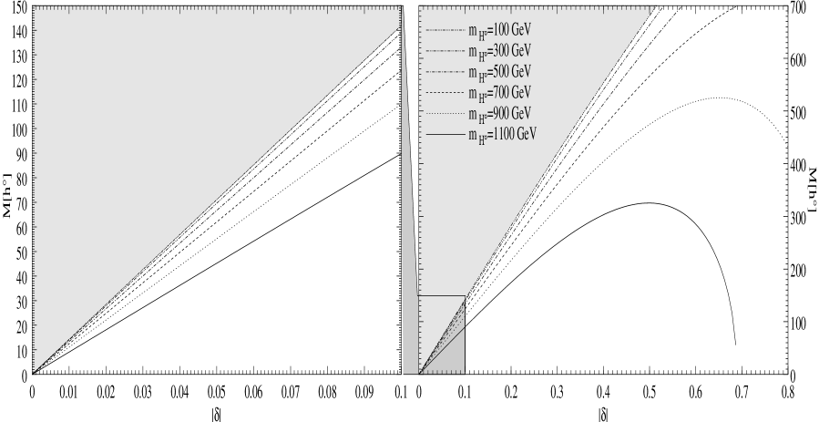
Figure 2: Limit on $m_{h^{0}}$ as a function of $\delta$ in potential$A$.

No tree-level unitarity bounds have been derived for potential $B$. A full derivation of these limits would be beyond the scope of this article. Nevertheless, we know that in the fermiophobic limit [5]:

$$m_{h^{0}}^{2}=m_{A}^{2}-2\left(\lambda_{+}-\lambda_{1}\right)v^{2}\cos^{2}\beta\enskip,$$ (7)

with $\lambda_{+}=\mbox{$\frac{1}{2}$}(\lambda_{3}+\lambda_{5})$ and $v=246\ GeV/c^{2}$ denoting the vacuum expectation value. The equation shows, that in the limit $\delta\rightarrow 0$ the masses of $h^{0}$ and $A^{0}$ will be degenerated. As already stated, stringent bounds on all $\lambda{{}_{i}}$´s are missing. On the other hand it might be sufficient to explore equation (7) for different values of $\lambda_{+}-\lambda_{1}\equiv\Delta\lambda$. Fig. 3 shows $m_{h^{0}}$ as a function of $\delta$ for different $\Delta\lambda$’s. On the left plot we set $m_{A}=80\ GeV$ and on the right plot $m_{A}=120\ GeV$. The region limited by each value of $|\Delta\lambda|$ is the allowed region for $m_{h^{0}}$ for the given value of $m_{A}$. Although it is most likely that $|\Delta\lambda|<10$, a value of $|\Delta\lambda|=100$ cannot strictly be excluded, if one wants to be very conservative.

Figure 3: Limit $m_{h^{0}}$ as a function of $\delta$ for $m_{A}=80\ GeV$ and $m_{A}=120\ GeV$.

In potential $B$, if $\delta\leq 0.05$, the masses of the lightest scalar and the pseudo-scalar are almost degenerated. $m_{h^{0}}$ can differ at most 15% from $m_{A}$, if $|\Delta\lambda|<10$. In the region where $0.05<|\delta|\leq 0.1$ the situation smoothly changes for the same $\Delta\lambda$. The restriction on the mass splitting vanishes totally when $\delta\gg 0.1$.

In potential $A$ we have an upper limit for $m_{h^{0}}$ independent of $m_{A}$. This upper bound depends on the value of $m_{H^{0}}$. It can be as low as $45\ GeV$ or reach a maximum of approximately $m_{W}$, if $\delta=0.05$. For $\delta=0.1$ the bound on $m_{h^{0}}$ varies between $90\ GeV$ and $140\ GeV$. Very stringent bounds on $m_{h^{0}}$ can be found, if $m_{H^{0}}$ is around $1\ TeV$ and $\delta$ is large. On the other hand for $m_{H^{0}}<700\ GeV$ no significant bounds can be found for a wide range of $\delta$ values.

We want to stress again (see [5]) that respecting these bounds is important to make reliable predictions on the decays of the Higgs particles of the 2HDM. Otherwise, one runs into spurious infinities of the couplings, which are not present in the original parameters of the potential.

These theoretical bounds and the overall picture given by the branching ratios shown in the next sections, led us to distinguish between three different regions for $\delta$. For our later qualitative analysis it is convenient to define the following regions:

• the tiny $\delta$ region where $|\delta|\leq 0.05$,

• the small $\delta$ region with $0.05<|\delta|\leq 0.1$ and

• finally the medium and large $\delta$ region when $|\delta|>0.1$.

5 The lightest scalar Higgs boson

As already pointed out, the lightest scalar Higgs boson ($h^{0}$) has no tree level couplings to the fermions for $\alpha=\pi/2$. Thus the following tree level decays have to be considered:

$$h^{0}\rightarrow W^{+}W^{-}\quad;\quad h^{0}\rightarrow ZZ\quad;\quad h^{0}\rightarrow ZA^{0}\quad;\quad h^{0}\rightarrow W^{\pm}H^{\mp}\quad;\quad h^{0}\rightarrow A^{0}A^{0}\quad;\quad h^{0}\rightarrow H^{+}H^{-}\quad.$$

Additionally the following one-loop induced decays are important:

$$h^{0}\rightarrow\gamma\gamma\quad;\quad h^{0}\rightarrow Z\gamma\quad;\quad h^{0}\rightarrow b\bar{b}\quad.$$

Moreover, decays to fermions via virtual vector bosons have to be taken into account, namely:

$$h^{0}\rightarrow W^{*}W^{*}\rightarrow f\bar{f}f\bar{f}\quad;\quad h^{0}\rightarrow W^{*}W\rightarrow f\bar{f}W\quad;\quad h^{0}\rightarrow Z^{*}Z^{*}\rightarrow f\bar{f}f\bar{f}\quad;\quad h^{0}\rightarrow Z^{*}Z\rightarrow f\bar{f}Z\quad.$$

The partial tree-level decay widths are listed in appendix A. The one-loop induced decays have been calculated with xloops [10]. Decays via virtual particles have been calculated in ref. [11]. We have taken these formulas and changed them appropriately. The decays into one vector boson and one scalar have been calculated in this paper for on-shell particles only. Near the thresholds decays via virtual particles (i.e. $h^{0}\rightarrow W^{*}H^{\pm}$ and $h^{0}\rightarrow Z^{*}A^{0}$) can be taken into account. These decays have been calculated in [12], where also formulas are given. The same applies to all other scalar particle decays calculated in the following sections.

As stated earlier, the only significant decay mode to fermions, via vector boson and scalar loops, is $h^{0}\rightarrow b\bar{b}$. For all the other fermionic decays the Feynman graphs are suppressed either by the Cabbibo-Kobayashi-Maskawa matrix or by the small mass of the fermions in the loop. However, the diagram shown in fig. 1 is suppressed by a $\tan^{2}\delta$ factor when compared with the corresponding diagram in $h^{0}\rightarrow\gamma\gamma$. Thus, as will be seen below, the decay $h^{0}\rightarrow b\bar{b}$ is of minor importance in the tiny and small $\delta$ region.

In potential $A$ the upper bound for the mass of the lightest scalar Higgs boson is approximately the $W$ mass in the tiny $\delta$ region. Thus $h^{0}$ has only two possible decay modes. Either it decays into $A^{0}A^{0}$, if the mass of the lightest scalar is twice as large as the mass of the pseudo-scalar Higgs boson, or it decays into two photons. In the small $\delta$ region the growth of the upper mass limit for $m_{h^{0}}$ gives rise to more decay modes, as can be seen in fig. 4. For small $h^{0}$ masses the situation is the same as in the tiny $\delta$ region. Depending on the mass of the pseudo-scalar, the dominant decay is again either $h^{0}\rightarrow A^{0}A^{0}$ or $h^{0}\rightarrow\gamma\gamma$. As soon as $m_{h^{0}}>m_{W}$, decays via virtual vector bosons overtake the decay to $\gamma\gamma$ and give rise to a fermionic signature of $h^{0}$. Of course the value of $m_{h^{0}}$, for which the branching ratio of $h^{0}\rightarrow W^{*}W^{*}$ becomes bigger than 50% depends on $\delta$. At the lower end of the small $\delta$ region this happens approximately at $m_{h^{0}}=110\ GeV$, whereas at the upper end it is close to the $W$ mass. At first, in the large $\delta$ region the branching ratio does not change much. Of course the upper bound for $m_{h^{0}}$ looses importance and all decays become kinematically allowed, as can be seen in fig. 5. As $\delta$ increases, the decay $h^{0}\rightarrow b\bar{b}$ becomes more and more significant for small masses of $m_{h^{0}}$. If e.g. $m_{h^{0}}=20\ GeV$ we get a branching ratio for $h^{0}\rightarrow b\bar{b}$ of the order of $30\%$ at $\delta=0.5$ and of $75\%$ at $\delta=1.0$. This reflects the already mentioned $\tan^{2}\delta$ suppression of this decay mode.

Figure 4: Branching ratios of $h^{0}$ at $m_{A^{0}}=70\ GeV$, $m_{H^{+}}=140\ GeV$, $m_{H^{0}}=300\ GeV$ and $\delta=0.1$ in potential $A$.

Figure 5: Branching ratios of $h^{0}$ at $m_{A^{0}}=120\ GeV$, $m_{H^{+}}=140\ GeV$, $m_{H^{0}}=300\ GeV$ and $\delta=0.2$ in potential $A$.

Figure 6: Branching ratios of $h^{0}$ at $m_{A^{0}}=m_{h^{0}}$, $m_{H^{+}}=140\ GeV$, $m_{H^{0}}=300\ GeV$ and $\delta=0.01$ in potential $B$.

Figure 7: Branching ratios of $h^{0}$ at $m_{A^{0}}=150\ GeV$, $m_{H^{+}}=210\ GeV$, $m_{H^{0}}=300\ GeV$ and $\delta=0.1$ in potential $B$.

In potential $B$ the masses of $h^{0}$ and $A^{0}$ are almost degenerated in the tiny $\delta$ region. Thus for small masses ($<m_{W}$) $h^{0}$ decays mainly into two photons. On the other hand, no upper bound on $m_{h^{0}}$ exists in potential $B$. As a consequence a heavy $h^{0}$ can also decay via virtual vector bosons into fermions in the tiny $\delta$ region (cf. fig. 6). In the small $\delta$ region the branching ratio strongly depends on the parameters $m_{A}$ and $m_{H^{+}}$. It can either resemble the plot for potential $A$ (see fig. 4), or, due to strong cancellation between the $H^{+}$- and the $W$-loops in the $h^{0}\rightarrow\gamma\gamma$ decay, it can be as shown in fig. 7. In this figure we see that $h^{0}\rightarrow\gamma\gamma$ only dominates until $m_{h^{0}}\approx 30\ GeV$. Then, decays via virtual vector bosons are the major decays of $h^{0}$. Note that $h^{0}\rightarrow b\bar{b}$ is suppressed in a similar way to $h^{0}\rightarrow\gamma\gamma$, because both decays depend on the same couplings of $h^{0}$ to the vector bosons and to the scalars. In the large $\delta$ region this behaviour is almost the same. Of course, as in potential $A$, for some value of $\delta$ the decay $h^{0}\rightarrow b\bar{b}$ will dominate over $h^{0}\rightarrow\gamma\gamma$ for small values of $m_{h^{0}}$.

Figure 8: Total decay width of $h^{0}$ with $m_{A^{0}}=130\ GeV$, $m_{H^{+}}=150\ GeV$, $m_{H^{0}}=300\ GeV$ for different values of $\delta$ potential $A$.

Finally we show the total branching ratio of $h^{0}$ as function of $m_{h^{0}}$ for different values of $\delta$ in fig. 8. As expected, the total decay width grows with $m_{h^{0}}$ and $\delta$. We do not show the total decay width for potential $B$ because the overall behaviour is the same as for potential $A$.

6 The pseudo-scalar Higgs boson

For our analysis the following tree level decays have to be considered:

$$A^{0}\rightarrow f\bar{f}\quad;\quad A^{0}\rightarrow Zh^{0}\quad;\quad A^{0}\rightarrow W^{\pm}H^{\mp}$$

Furthermore the following one-loop decays have been calculated:

$$A^{0}\rightarrow\gamma\gamma\quad;\quad A^{0}\rightarrow Z\gamma\quad;\quad A^{0}\rightarrow W^{+}W^{-}\quad;\quad A^{0}\rightarrow ZZ\quad;\quad A^{0}\rightarrow gg\quad,$$

where $g$ denotes a gluon.

Leaving aside the tree level decays into a final state with at least one Higgs particles, all decays depend on the coupling of $A^{0}$ to the fermions ($\cot^{2}\beta$ in model I). This is a consequence of the fact that without fermions $CP$ conservation is equivalent to separate $C$ and $P$ conservation. So, no on-shell decay with only vector bosons in the final state is possible. When the fermions are included, $C$ and $P$ are no longer independently conserved, and so $A^{0}$ can decay into two photons, for instance, via a fermion loop.

Figure 9: Branching ratios of $A^{0}$ as a function of the mass for $\delta=0.1$, $m_{h^{0}}=55\ GeV$, $m_{H^{0}}=300\ GeV$ and $m_{H^{+}}=130\ GeV$.

Figure 10: Branching ratios as a function of $\delta$ for $m_{A^{0}}=190\ GeV$, $m_{h^{0}}=55\ GeV$, $m_{H^{0}}=300\ GeV$ and $m_{H^{+}}=100\ GeV$.

Figure 11: Travel distance of $A^{0}$ at $\sqrt{s}=189\ GeV$ and $m_{h^{0}}=10\ GeV$.

On the other hand, when fermions are added, $A^{0}$ may directly decay into them. As these are tree-level decays, their partial decay widths are obviously larger than one-loop induced decay widths. This can also be seen in fig. 9. This figure clearly shows, that the one-loop decays of the pseudo-scalar Higgs are in the per mille region when compared to the fermionic decays. We have checked that the $A^{0}$ branching ratio is independent of $\delta$ below $Zh^{0}$ and $W^{\pm}H^{\mp}$ thresholds. As we have pointed out, in this region all decays just depend on $\cot\beta$. This dependence cancels in the branching ratios, but not in the decay width. Above these thresholds $A^{0}$ decays mainly into $Zh^{0}$ and $W^{\pm}H^{\mp}$, as can be seen in fig. 10. Only in the very large $\delta$ region the decays into fermions dominate due to the dependence on $\tan\delta$.

Although below the $Zh^{0}$ and the $W^{\pm}H^{\mp}$ thresholds $A^{0}$ decays mainly into fermions, the total decay width of $A^{0}$ decreases with $\tan^{2}\delta$ in this region. So in the limit $\delta\rightarrow 0$ the pseudo-scalar Higgs will be a stable particle leaving no characteristic signature in the detector. Furthermore, for a sufficiently small $\delta$, $A^{0}$ decays outside the detector (see fig. 11). So, the only way to detect it in this $\delta$ region is to consider reactions with missing energy and momentum in the final state. The situation changes, as soon as the $Zh^{0}$ or the $W^{\pm}H^{\mp}$ thresholds are crossed. Then $A^{0}$ decays inside the detector with either a $Zh^{0}$ or a $W^{\pm}H^{\mp}$ signature.

Finally we notice, that all decays either depend on the coupling of $A^{0}$ to fermions or to vector bosons. There is no decay, where couplings of the scalars among themselves contribute to the decay width. Thus for the pseudo-scalar Higgs boson no difference between potential $A$ and $B$ can be seen in the branching ratios and decay widths. So, the signature of the $A^{0}$ may be called Higgs potential independent.

7 The charged Higgs boson

Figure 12: Branching ratios for $H^{+}$ at $\delta=0.01$, $m_{A^{0}}=80\ GeV$, $m_{h^{0}}=20\ GeV$ and $m_{H^{0}}=300\ GeV$ in potential $A$.

Figure 13: Branching ratios for $H^{+}$ at $\delta=0.01$, $m_{A^{0}}=80\ GeV$, $m_{h^{0}}=78\ GeV$ and $m_{H^{0}}=500\ GeV$ in potential $B$.

Figure 14: Branching ratios for $H^{+}$ at $\delta=0.01$, $m_{A^{0}}=80.1\ GeV$, $m_{h^{0}}=80\ GeV$ and $m_{H^{0}}=500\ GeV$ in potential $B$.

The charged Higgs boson has the following tree-level decays:

$$H^{\pm}\rightarrow f_{u,d}\bar{f}_{d,u}\quad;\quad H^{\pm}\rightarrow W^{\pm}h^{0}\quad;\quad H^{\pm}\rightarrow W^{\pm}A^{0}\quad;\quad H^{\pm}\rightarrow W^{\pm}H^{0}$$

Moreover the following one-loop decays have to be considered:

$$H^{\pm}\rightarrow W^{\pm}\gamma\quad;\quad H^{\pm}\rightarrow W^{\pm}Z$$

Again, the 16 (32) graphs for $H^{\pm}\rightarrow W^{\pm}\gamma$ ($H^{\pm}\rightarrow W^{\pm}Z$) have been calculated with xloops [10].

In potential $A$ the branching ratios of the charged Higgs boson show no surprises (fig. 12). If the mass of $H^{\pm}$ is below the $W$ mass the signature will be fermionic and independent of the value of $\delta$. In this mass region the situation is similar to the former situation concerning the pseudo-scalar Higgs boson. Decreasing $\delta$ just decreases the total decay width, but leaves the branching ratio unchanged. The situation changes, as soon as the $W\gamma$ threshold is passed. Then, in the tiny $\delta$ region the signature will be $H^{\pm}\rightarrow W^{\pm}\gamma$. In the small $\delta$ region, as $\delta$ grows the branching ratio of $H^{\pm}\rightarrow W^{\pm}\gamma$ decreases to less than 1%. Consequently in the large $\delta$ region the signature is again fermionic. As soon as decays to the $W$ and either $A^{0}$ or $h^{0}$ are kinematically allowed, the sum of these decays will have an approximately 100% branching ratio for almost all values of $\delta$. Only if $\delta$ becomes very large and $m_{H^{+}}>m_{t}+m_{b}$ the decay $H^{+}\rightarrow t\bar{b}$ will be the dominant decay mode.

In potential $B$ below the $W\gamma$ and above the $Wh^{0}$ or $WA^{0}$ threshold the situation is the same as in potential $A$. When the decay $H^{\pm}\rightarrow W^{\pm}\gamma$ is important, the situation strongly depends on the choice of parameters. In principle, due to the lack of an upper bound for $m_{h^{0}}$ in potential $B$, the interval of $m_{H^{+}}$, where $H^{\pm}\rightarrow W^{\pm}\gamma$ could be much larger than in potential $A$. On the other hand, it turns out that due to the degeneracy of $m_{h^{0}}$ and $m_{A^{0}}$ the decay to $W\gamma$ can be suppressed to a few percent in comparison to the fermion decays (see fig. 14). This behaviour can also be seen for very tiny values of $\delta$. If the restriction on $m_{A^{0}}$ and $m_{h^{0}}$ is limbered and their masses just differ by a few $GeV$, $H^{\pm}\rightarrow W^{\pm}\gamma$ regains its importance (fig. 13). Moreover, in contrast to potential $A$, it can still be the major decay in the small and at the start of the large $\delta$ region. Even for $\delta=0.2$ the branching of $H^{\pm}\rightarrow W^{\pm}\gamma$ can reach up to 10%, if the masses of the Higgs sector are chosen appropriately. Of course for an even larger value of $\delta$ the branching ratio for this decay mode will become unimportant.

8 The heavy scalar Higgs boson

Figure 15: Branching ratios for $H^{0}$ at $\delta=0.1$ in potential $A$.

Figure 16: Branching ratios for $H^{0}$ at $\delta=0.5$ in potential $B$.

For the sake of completeness we show the decay modes of the heavy scalar Higgs boson, although its coupling to the fermions is large. Thus one-loop decays have no importance in the branching ratio of $H^{0}$. So we just consider the following tree-level decays:

$$\begin{array}[]{lclclclc}H^{0}\rightarrow f\bar{f}&;&H^{0}\rightarrow H^{+}H^{-}&;&H^{0}\rightarrow A^{0}A^{0}&;&&\\ H^{0}\rightarrow W^{\pm}H^{\mp}&;&H^{0}\rightarrow ZA^{0}&;&H^{0}\rightarrow ZZ&;&H^{0}\rightarrow W^{+}W^{-}&\end{array}$$

Note that the decay $H^{0}\rightarrow h^{0}h^{0}$ vanishes in the fermiophobic limit (i.e. for $\alpha=\pi/2$).

A typical plot of the branching ratio as a function of the mass is shown in fig. 15. Obviously, the heavy scalar Higgs boson mainly decays into $b\bar{b}$ below, and into $WW$ above the two vector boson threshold. This behaviour is typical for both potentials. The only difference between the potentials can be recognized in the purely scalar decay modes. In potential $A$ their contribution varies from $0\%$ to $\approx 20\%$ depending on the parameters chosen. In potential $B$ the decay $H^{0}\rightarrow H^{+}H^{-}$ can be the major decay mode for some values of $\delta$, $m_{H^{+}}$ and $m_{A}$, as can be seen in fig. 16.

Only if $\delta>1.0$, $H^{0}$ mainly decays to $t\bar{t}$. Notice that the branching ratios shown in fig. 15 are similar those obtained for the SM Higgs boson, if the scalar decays are ignored.

9 Constraints on the models

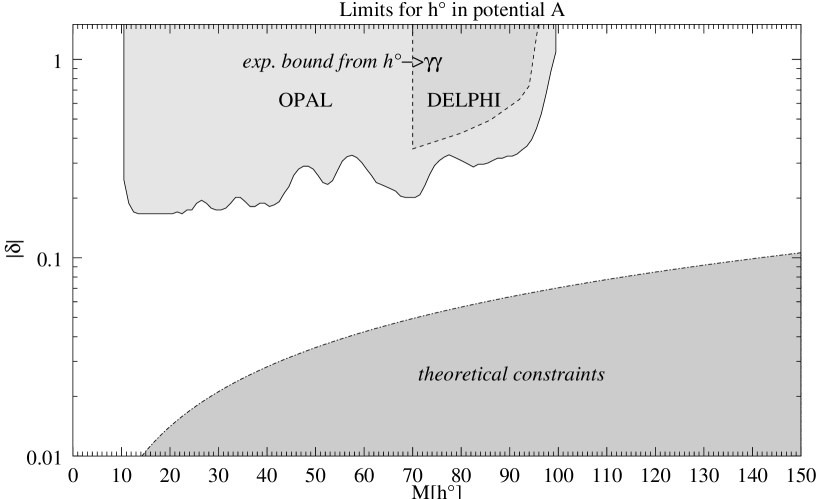
Figure 17: Bounds in the $m_{h^{0}}$-$\delta$ plane for potential $A$.

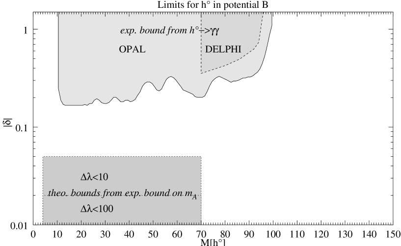
Figure 18: Bounds in the $m_{h^{0}}$-$\delta$ plane for potential $B$.

In this section we use the available experimental data and the bounds derived in section 4 to constrain the models.

Most production modes of the pseudo-scalar Higgs boson at LEP are suppressed in the fermiophobic limit. An exception is the associated production $Z^{*}\rightarrow h^{0}A^{0}$ when kinematically allowed. The more $\delta$ tends to zero the larger becomes the cross section for this production mode. However, the obtained limit for $m_{A}$ is not independent of the mass of the lightest scalar Higgs boson. This production mechanism has recently been measured by the DELPHI coll. [13], where more detailed results can be found. For this associated production we roughly summarize their result in the following inequation:

$$\sqrt{m_{h^{0}}^{2}+m_{A}^{2}}\geq 80\ GeV$$ (8)

For the lightest scalar Higgs boson mass the most stringent bounds can be derived from the experimental measurement of massive di-photon resonances. The most recent data have been published in refs. [14, 13]. We have used this data to exclude some regions in the $m_{h^{0}}$-$\delta$ plane. We have plotted the results in fig. 17 for potential $A$ and in fig. 18 for potential $B$. Moreover we have inserted the theoretical constraints shown in fig. 2. In fig. 17 (potential $A$) this can be seen as the lower limit on $\delta$ for a given $h^{0}$ mass. For potential $B$ the experimental bound on $m_{A}$ can be used to derive a lower limit on $\delta$ for a given $m_{h^{0}}$. In fig. 18 we have plotted this area for different values of $\Delta\lambda$.

Model independent bounds for the charged Higgs boson mass can be obtained using the universality of the electromagnetic coupling. Measurements of $e^{+}e^{-}\rightarrow H^{+}H^{-}$ at LEP currently yield a lower bound of $m_{H^{+}}>59\ GeV$ [15]. In hadron colliders the search for $t\rightarrow H^{+}b$ gives a limit of $Br(t\rightarrow H^{+}b)\times Br(H^{+}\rightarrow\tau\nu_{\tau})\leq 50\%$ if $60\ GeV\leq m_{H^{+}}\leq 165\ GeV$ [16]. This imposes a lower as well as an upper limit on $\beta$ in 2HDM’s with coupling to fermions of type II or III. Unfortunately, in the 2HDM I this simply gives a very large upper limit on $\delta$, but no lower limit. Furthermore, we have shown in section 7 that for $m_{H^{+}}>m_{W}$ the decay $H^{+}\rightarrow\tau\nu_{\tau}$ can be suppressed in the fermiophobic limit.

10 Conclusion and outlook

We have calculated the branching ratios for all Higgs particles of fermiophobic 2HDM´s as a function of the Higgs masses and $\delta$. We have shown that the two different scalar sectors, models $A$ and $B$, give rise to different signatures for some regions of the parameter space. Most of the mass bounds based on a general 2HDM or on the MSSM do not apply in the fermiophobic case. We have used the available experimental data and tree-level unitarity bounds to constrain the models. It turns out, that there is still a wide region of this parameter space not yet excluded by experimental data and still accessible at the LEP collider. So, one should keep an open mind for surprises in the Higgs sector.

11 Acknowledgement

We would like to thank our experimental colleagues at LIP for inspiring discussions and A. Barroso for a careful reading of the manuscript. L.B. is supported by JNICT under contract No. BPD.16372.

Appendix A Formulas for the decay widths

Here we present the most important formulas for the decay widths of the Higgs particles. We use the Kallen function $\lambda(x,y,z)=x^{2}+y^{2}+z^{2}-2xy-2xz-2yz$ in the formulas below. For the lightest scalar the following tree-level decays have been calculated:

$$\Gamma(h^{0}\rightarrow W^{+}W^{-}) = \frac{g^{2}\,m_{W}^{2}\sin^{2}\delta}{8\pi\,m_{h^{0}}^{2}}\,\sqrt{m_{h^{0}}^{2}-4m_{W}^{2}}\,\left[\,1\,+\,\frac{\left(m_{h^{0}}^{2}-2m_{W}^{2}\right)^{2}}{8\,m_{W}^{4}}\,\right]$$

$$\Gamma(h^{0}\rightarrow ZZ) = \frac{g^{2}\,m_{Z}^{4}\cos^{2}\delta}{16\pi\,m_{W}^{2}m_{h^{0}}^{2}}\,\sqrt{m_{h^{0}}^{2}-4m_{Z}^{2}}\,\left[\,1\,+\,\frac{\left(m_{h^{0}}^{2}-2m_{Z}^{2}\right)^{2}}{8\,m_{Z}^{4}}\,\right]$$

$$\Gamma(h^{0}\rightarrow ZA^{0}) = \frac{g^{2}\cos^{2}\delta}{64\pi\,m_{W}^{2}m_{h^{0}}^{3}}\lambda^{\frac{3}{2}}\left(m_{h^{0}}^{2},m_{A^{0}}^{2},m_{Z}^{2}\right)$$

$$\Gamma(h^{0}\rightarrow W^{\pm}H^{\mp}) = \frac{g^{2}\cos^{2}\delta}{64\pi\,m_{h^{0}}^{3}m_{W}^{2}}\lambda^{\frac{3}{2}}(m_{h^{0}}^{2},m_{H^{+}}^{2},m_{W}^{2})$$

$$\Gamma^{(A/B)}(h^{0}\rightarrow A^{0}A^{0}) = \frac{\sqrt{m_{h^{0}}^{2}-4m_{A^{0}}^{2}}}{32\pi\,m_{h^{0}}^{2}}\,\left|C^{(A/B)}_{[h^{0}A^{0}A^{0}]}\right|^{2}$$

$$\Gamma^{(A/B)}(h^{0}\rightarrow H^{+}H^{-}) = \frac{\sqrt{m_{h^{0}}^{2}-4m_{H^{+}}^{2}}}{16\pi\,m_{h^{0}}^{2}}\,\left|C^{(A/B)}_{[h^{0}H^{+}H^{-}]}\right|^{2}\qquad\qquad.$$

The couplings $C^{(A/B)}_{[h^{0}H^{+}H^{-}]}$ for either potential $A$ or potential $B$ are listed in appendix B. The one-loop decays have been automatically calculated with xloops. Unfortunately the formulas are to large to be shown here. A compact formula for $h^{0}\rightarrow\gamma\gamma$ in the MSSM can be found in ref. [17].

For the pseudo-scalar Higgs boson one gets:

$$\Gamma(A^{0}\rightarrow f\bar{f}) = N_{c}\frac{g^{2}m_{f}^{2}\cot^{2}\beta}{32\pi m_{W}^{2}}\sqrt{\frac{m_{A^{0}}^{2}}{4}-m_{f}^{2}}\left[1-\frac{4m_{f}^{2}}{m_{A^{0}}^{2}}\right]$$

$$\Gamma(A^{0}\rightarrow Zh^{0}) = \frac{g^{2}\cos^{2}\delta}{64\pi\,m_{W}^{2}m_{A^{0}}^{3}}\lambda^{\frac{3}{2}}\left(m_{A^{0}}^{2},m_{h^{0}}^{2},m_{Z}^{2}\right)$$

$$\Gamma(A^{0}\rightarrow W^{\pm}H^{\mp}) = \frac{g^{2}}{64\pi\,m_{W}^{2}m_{A^{0}}^{3}}\lambda^{\frac{3}{2}}\left(m_{A^{0}}^{2},m_{H^{+}}^{2},m_{W}^{2}\right)$$

$$\Gamma(A^{0}\rightarrow\gamma\gamma) = \frac{m_{A^{0}}^{3}}{32\pi}\left|\frac{N_{c}{e}^{3}m_{t}^{2}\cot\beta}{9\,\sin\theta_{W}\,m_{W}\,{\pi}^{4}}\mbox{Oneloop3Pt}\left(0,0,0,m_{A^{0}},\mbox{$\frac{1}{2}$}m_{A^{0}},\mbox{$\frac{1}{2}$}m_{A^{0}},m_{t},m_{t},m_{t}\right)\right|^{2}$$

$N_{c}$ denotes the number of quark colors. Beside $A^{0}\rightarrow\gamma\gamma$ all other formulas for one-loop decays have been skipped. The definition of the OneLoop3Pt function can be found in ref. [18]. An ${\cal O}({\alpha}_{s})$ improved formula for $\Gamma(A^{0}\rightarrow q\bar{q})$ can be found in ref. [19].

The charged Higgs boson has the following partial decay widths:

$$\Gamma(H^{+}\rightarrow f_{t}\bar{f_{b}}) = \frac{g^{2}\cot^{2}\beta\,N_{c}\left|V_{tb}\right|^{2}}{64\pi\,m_{W}^{2}}\frac{\lambda^{\frac{1}{2}}(m_{H^{+}}^{2},m_{t}^{2},m_{b}^{2})}{m_{H^{+}}^{3}}\left[\left(m_{H^{+}}^{2}-m_{t}^{2}-m_{b}^{2}\right)\left(m_{t}^{2}+m_{b}^{2}\right)+4\,m_{t}^{2}m_{b}^{2}\right]$$

$$\Gamma(H^{+}\rightarrow W^{+}h^{0}) = \frac{g^{2}\cos^{2}\delta}{64\pi\,m_{H^{+}}^{3}m_{W}^{2}}\lambda^{\frac{3}{2}}(m_{H^{+}}^{2},m_{h^{0}}^{2},m_{W}^{2})$$

$$\Gamma(H^{+}\rightarrow W^{+}A^{0}) = \frac{g^{2}}{64\pi\,m_{H^{+}}^{3}m_{W}^{2}}\lambda^{\frac{3}{2}}(m_{H^{+}}^{2},m_{A^{0}}^{2},m_{W}^{2})$$

$$\Gamma(H^{+}\rightarrow W^{+}H^{0}) = \frac{g^{2}\sin^{2}\delta}{64\pi\,m_{H^{+}}^{3}m_{W}^{2}}\lambda^{\frac{3}{2}}(m_{H^{+}}^{2},m_{H^{0}}^{2},m_{W}^{2})$$

Note that $\Gamma(H^{+}\rightarrow f_{t}\bar{f_{b}})$ is also valid for leptons with $m_{\nu}\equiv m_{t}=0$ and $N_{c}=1$. Again we skip the formula for $H^{+}\rightarrow W^{+}\gamma$ and $H^{+}\rightarrow W^{+}Z$ due to its length.

For the heavy Higgs boson ($H^{0}$) we calculate:

$$\Gamma(H^{0}\rightarrow f\bar{f}) = \frac{g^{2}\,N_{c}\,m_{f}^{2}\,\sin^{2}\alpha}{64\pi\,m_{W}^{2}\sin^{2}\beta}\,\sqrt{m_{H^{0}}^{2}-4m_{f}^{2}}$$

$$\Gamma(H^{0}\rightarrow W^{+}W^{-}) = \frac{g^{2}\,m_{W}^{2}\cos^{2}\delta}{8\pi\,m_{H^{0}}^{2}}\,\sqrt{m_{H^{0}}^{2}-4m_{W}^{2}}\,\left[\,1\,+\,\frac{\left(m_{H^{0}}^{2}-2m_{W}^{2}\right)^{2}}{8\,m_{W}^{4}}\,\right]$$

$$\Gamma(H^{0}\rightarrow ZZ) = \frac{g^{2}\,m_{Z}^{4}\cos^{2}\delta}{16\pi\,m_{W}^{2}m_{H^{0}}^{2}}\,\sqrt{m_{H^{0}}^{2}-4m_{Z}^{2}}\,\left[\,1\,+\,\frac{\left(m_{H^{0}}^{2}-2m_{Z}^{2}\right)^{2}}{8\,m_{Z}^{4}}\,\right]$$

$$\Gamma(H^{0}\rightarrow ZA^{0}) = \frac{g^{2}\sin^{2}\delta}{64\pi\,m_{W}^{2}m_{H^{0}}^{3}}\lambda^{\frac{3}{2}}\left(m_{H^{0}}^{2},m_{A^{0}}^{2},m_{Z}^{2}\right)$$

$$\Gamma(H^{0}\rightarrow W^{\pm}H^{\mp}) = \frac{g^{2}\sin^{2}\delta}{64\pi\,m_{H^{0}}^{3}m_{W}^{2}}\lambda^{\frac{3}{2}}(m_{H^{0}}^{2},m_{H^{+}}^{2},m_{W}^{2})$$

$$\Gamma^{(A/B)}(H^{0}\rightarrow A^{0}A^{0}) = \frac{\sqrt{m_{H^{0}}^{2}-4m_{A^{0}}^{2}}}{32\pi\,m_{H^{0}}^{2}}\,\left|C^{(A/B)}_{[H^{0}A^{0}A^{0}]}\right|^{2}$$

$$\Gamma^{(A/B)}(H^{0}\rightarrow H^{+}H^{-}) = \frac{\sqrt{m_{H^{0}}^{2}-4m_{H^{+}}^{2}}}{16\pi\,m_{H^{0}}^{2}}\,\left|C^{(A/B)}_{[H^{0}H^{+}H^{-}]}\right|^{2}$$

Appendix B Feynman rules

In this section we present the Feynman rules for the triple and quartic interactions of scalar fields which are different in both potentials. A full treatment of all Feynman rules will be found in ref. [20].

We define the following quantities:
$\displaystyle A_{\alpha\beta}$ $\displaystyle\equiv$ $\displaystyle\cos^{3}\beta\sin\alpha+\sin^{3}\beta\cos\alpha$ $\displaystyle B_{\alpha\beta}$ $\displaystyle\equiv$ $\displaystyle\cos^{3}\beta\cos\alpha-\sin^{3}\beta\sin\alpha$ $\displaystyle C_{\alpha\beta}$ $\displaystyle\equiv$ $\displaystyle\sin^{3}\alpha\cos\beta+\cos^{3}\alpha\sin\beta$ $\displaystyle D_{\alpha\beta}$ $\displaystyle\equiv$ $\displaystyle\cos^{3}\alpha\cos\beta-\sin^{3}\alpha\sin\beta$ $\displaystyle E_{\alpha\beta}$ $\displaystyle\equiv$ $\displaystyle(\cos^{2}\alpha-\sin^{2}\beta)$ $\displaystyle F_{\alpha\beta}$ $\displaystyle\equiv$ $\displaystyle(\cos^{2}\alpha-\cos^{2}\beta)$ $\displaystyle G_{\alpha\beta}$ $\displaystyle\equiv$ $\displaystyle\cos\beta\sin\beta-3\cos\alpha\sin\alpha$ $\displaystyle H_{\alpha\beta}$ $\displaystyle\equiv$ $\displaystyle\cos 2\beta\cos\delta\cos(\alpha+\beta)$ $\displaystyle K_{\alpha\beta}$ $\displaystyle\equiv$ $\displaystyle\cos 2\beta(\cos^{2}\alpha-\cos^{2}\beta)$

B.1 Different triple scalar vertices in $V_{A}$

$H^{+}H^{-}h$	$-\frac{ig}{M_{W}}\left(\frac{M_{h}^{2}}{\sin 2\beta}B_{\alpha\beta}-M_{H^{+}}^{2}\sin\delta\right)$
$H^{+}H^{-}H$	$-\frac{ig}{M_{W}}\left(\frac{M_{H}^{2}}{\sin 2\beta}A_{\alpha\beta}+M_{H^{+}}^{2}\cos\delta\right)$
$hHH$	$-\frac{ig}{2M_{W}}\frac{\sin 2\alpha\sin\delta}{\sin 2\beta}(2M_{H}^{2}+M_{h}^{2})$
$hhH$	$-\frac{ig}{2M_{W}}\frac{\sin 2\alpha\cos\delta}{\sin 2\beta}(M_{H}^{2}+2M_{h}^{2})$

$hhh$	$-\frac{3ig}{M_{W}}\frac{M_{h}^{2}}{\sin 2\beta}D_{\alpha\beta}$
$HHH$	$-\frac{3ig}{M_{W}}\frac{M_{H}^{2}}{\sin 2\beta}C_{\alpha\beta}$
$AAh$	$-\frac{ig}{M_{W}}\left(\frac{M_{h}^{2}}{\sin 2\beta}B_{\alpha\beta}-M_{A}^{2}\sin\delta\right)$
$AAH$	$-\frac{ig}{M_{W}}\left(\frac{M_{H}^{2}}{\sin 2\beta}A_{\alpha\beta}+M_{A}^{2}\cos\delta\right)$

B.2 Different triple scalar vertices in $V_{B}$

$H^{+}H^{-}h$	$-\frac{ig}{M_{W}}\left(\frac{M_{h}^{2}}{\sin 2\beta}B_{\alpha\beta}-M_{H^{+}}^{2}\sin\delta-\frac{\cos\delta}{\sin 2\beta}M_{A}^{2}\right)$
$H^{+}H^{-}H$	$-\frac{ig}{M_{W}}\left(\frac{M_{H}^{2}}{\sin 2\beta}A_{\alpha\beta}+M_{H^{+}}^{2}\cos\delta+\frac{\sin\delta}{\sin 2\beta}M_{A}^{2}\right)$
$hHH$	$-\frac{ig\sin\delta}{2M_{W}\sin 2\beta}\left(\sin 2\alpha(2M_{H}^{2}+M_{h}^{2})+M_{A}^{2}G_{\alpha\beta}\right)$
$hhH$	$-\frac{ig\cos\delta}{2M_{W}\sin 2\beta}\left(\sin 2\alpha(M_{H}^{2}+2M_{h}^{2})+M_{A}^{2}G_{\alpha\beta}\right)$

$hhh$	$-\frac{3ig}{M_{W}\sin 2\beta}\left(M_{h}^{2}D_{\alpha\beta}-M_{A}^{2}\,E_{\alpha\beta}\cos\delta\,\right)$
$HHH$	$-\frac{3ig}{M_{W}\sin 2\beta}\left(M_{H}^{2}C_{\alpha\beta}+M_{A}^{2}\,F_{\alpha\beta}\sin\delta\,\right)$
$AAh$	$-\frac{ig}{M_{W}}\left(\frac{M_{h}^{2}}{\sin 2\beta}B_{\alpha\beta}-M_{A}^{2}\frac{\cos\delta\cos 2\beta}{\sin 2\beta}\right)$
$AAH$	$-\frac{ig}{M_{W}}\left(\frac{M_{H}^{2}}{\sin 2\beta}A_{\alpha\beta}-M_{A}^{2}\frac{\sin\delta\cos 2\beta}{\sin 2\beta}\right)$

B.3 Different quartic scalar vertices for $V_{A}$

$H^{+}H^{-}H^{+}H^{-}$		$-\frac{2\,ig^{2}}{\sin^{2}2\beta M_{W}^{2}}(M_{H}^{2}A_{\alpha\beta}^{2}+M_{h}^{2}B_{\alpha\beta}^{2})$
$AAAA$		$-\frac{3ig^{2}}{\sin^{2}2\beta M_{W}^{2}}(M_{H}^{2}A_{\alpha\beta}^{2}+M_{h}^{2}B_{\alpha\beta}^{2})$
$AAH^{+}H^{-}$		$-\frac{ig}{\sin^{2}2\beta M_{W}^{2}}(M_{H}^{2}A_{\alpha\beta}^{2}+M_{h}^{2}B_{\alpha\beta}^{2})$
$H^{+}H^{-}hh$		$-\frac{ig^{2}}{2M_{W}^{2}}\left[\frac{1}{\sin^{2}2\beta}(M_{H}^{2}A_{\alpha\beta}\sin 2\alpha\cos\delta+2M_{h}^{2}B_{\alpha\beta}D_{\alpha\beta})+M_{H^{+}}^{2}\sin^{2}\delta\right]$
$H^{+}H^{-}HH$		$-\frac{ig^{2}}{2M_{W}^{2}}\left[\frac{1}{\sin^{2}2\beta}(2M_{H}^{2}A_{\alpha\beta}C_{\alpha\beta}+M_{h}^{2}B_{\alpha\beta}\sin 2\alpha\sin\delta)+M_{H^{+}}^{2}\cos^{2}\delta\right]$
$AAhh$		$-\frac{ig^{2}}{2M_{W}^{2}}\left[\frac{1}{\sin^{2}2\beta}(M_{H}^{2}A_{\alpha\beta}\sin 2\alpha\cos\delta+2M_{h}^{2}B_{\alpha\beta}D_{\alpha\beta})+M_{A}^{2}\sin^{2}\delta\right]$
$AAHH$		$-\frac{ig^{2}}{2M_{W}^{2}}\left[\frac{1}{\sin^{2}2\beta}(2M_{H}^{2}A_{\alpha\beta}C_{\alpha\beta}+M_{h}^{2}B_{\alpha\beta}\sin 2\alpha\sin\delta)+M_{A}^{2}\cos^{2}\delta\right]$
$H^{+}H^{-}Hh$		$-\frac{ig^{2}}{2M_{W}^{2}}\left[\frac{\sin 2\alpha}{\sin^{2}2\beta}(M_{H}^{2}A_{\alpha\beta}\sin\delta+M_{h}^{2}B_{\alpha\beta}\cos\delta)-\frac{1}{2}M_{H^{+}}^{2}\sin 2\delta\right]$
$AAHh$		$-\frac{ig^{2}}{2M_{W}^{2}}\left[\frac{\sin 2\alpha}{\sin^{2}2\beta}(M_{H}^{2}A_{\alpha\beta}\sin\delta+M_{h}^{2}B_{\alpha\beta}\cos\delta)-\frac{1}{2}M_{A}^{2}\sin 2\delta\right]$
$hhhh$		$-\frac{3\,ig^{2}}{\sin^{2}2\beta M_{w}^{2}}(4M_{h}^{2}D_{\alpha\beta}^{2}+M_{H}^{2}\sin^{2}2\alpha\cos^{2}\delta)$
$HHHH$		$-\frac{3\,ig^{2}}{\sin^{2}2\beta M_{W}^{2}}(M_{h}^{2}\sin^{2}2\alpha\sin^{2}\delta+4M_{H}^{2}C_{\alpha\beta}^{2})$
$hhhH$		$-\frac{3\,ig^{2}}{2\sin^{2}2\beta M_{W}^{2}}(4M_{h}^{2}D_{\alpha\beta}\sin 2\alpha\cos\delta+M_{H}^{2}\sin^{2}2\alpha\sin 2\delta)$
$HHHh$		$-\frac{3ig^{2}}{2\sin^{2}2\beta M_{W}^{2}}(M_{h}^{2}\sin^{2}2\alpha\sin 2\delta+4M_{H}^{2}C_{\alpha\beta}\sin 2\alpha\sin\delta)$
$hhHH$		$-\frac{ig^{2}\sin 2\alpha}{4\sin 2\beta M_{W}^{2}}\left[M_{H}^{2}-M_{h}^{2}+\frac{3\sin 2\alpha}{\sin 2\beta}(\sin^{2}\delta M_{H}^{2}+\cos^{2}\delta M_{h}^{2})\right]$
$AAG^{0}G^{0}$		$-\frac{ig^{2}}{4M_{W}^{2}}\left[\frac{\sin 2\alpha}{\sin 2\beta}(M_{H}^{2}-M_{h}^{2})+3(\sin^{2}\delta M_{H}^{2}+\cos^{2}\delta M_{h}^{2})\right]$
$H^{+}H^{-}G^{+}G^{-}$		$-\frac{ig^{2}}{4M_{W}^{2}}\left[M_{A}^{2}+\frac{\sin 2\alpha}{\sin 2\beta}(M_{H}^{2}-M_{h}^{2})+2(\sin^{2}\delta M_{H}^{2}+\cos^{2}\delta M_{h}^{2})\right]$

$G^{+}G^{-}AA$		$-\frac{ig^{2}}{2M_{W}^{2}}\left[M_{H^{+}}^{2}+\frac{1}{\sin 2\beta}(\cos\delta A_{\alpha\beta}M_{H}^{2}-\sin\delta B_{\alpha\beta}M_{h}^{2})\right]$
$H^{+}H^{-}G^{0}G^{0}$		$-\frac{ig^{2}}{2M_{W}^{2}}\left[M_{H^{+}}^{2}+\frac{1}{\sin 2\beta}(\cos\delta A_{\alpha\beta}M_{H}^{2}-\sin\delta B_{\alpha\beta}M_{h}^{2})\right]$
$H^{+}H^{-}H^{\mp}G^{\pm}$		$-\frac{ig^{2}}{M_{W}^{2}\sin 2\beta}\left[\sin\delta A_{\alpha\beta}M_{H}^{2}+\cos\delta B_{\alpha\beta}M_{h}^{2}\right]$
$H^{+}H^{-}G^{0}A$		$-\frac{ig^{2}}{2M_{W}^{2}\sin 2\beta}\left[\sin\delta A_{\alpha\beta}M_{H}^{2}+\cos\delta B_{\alpha\beta}M_{h}^{2}\right]$
$AAAG^{0}$		$-\frac{3\,ig^{2}}{2M_{W}^{2}\sin 2\beta}\left[\sin\delta A_{\alpha\beta}M_{H}^{2}+\cos\delta B_{\alpha\beta}M_{h}^{2}\right]$
$AAH^{\mp}G^{\pm}$		$-\frac{ig^{2}}{2M_{W}^{2}\sin 2\beta}\left[\sin\delta A_{\alpha\beta}M_{H}^{2}+\cos\delta B_{\alpha\beta}M_{h}^{2}\right]$
$G^{+}G^{-}hh$		$-\frac{ig^{2}}{4M_{W}^{2}}\left[\frac{1}{\sin 2\beta}(\sin 2\alpha\cos^{2}\delta M_{H}^{2}-2\sin\delta D_{\alpha\beta}M_{h}^{2})+2\cos^{2}\delta M_{H^{+}}^{2}\right]$
$G^{0}G^{0}hh$		$-\frac{ig^{2}}{4M_{W}^{2}}\left[\frac{1}{\sin 2\beta}(\sin 2\alpha\cos^{2}\delta M_{H}^{2}-2\sin\delta D_{\alpha\beta}M_{h}^{2})+2\cos^{2}\delta M_{A}^{2}\right]$
$G^{+}G^{-}HH$		$-\frac{ig^{2}}{4M_{W}^{2}}\left[\frac{1}{\sin 2\beta}(2\cos\delta C_{\alpha\beta}M_{H}^{2}-\sin^{2}\delta\sin 2\alpha M_{h}^{2})+2\sin^{2}\delta M_{H^{+}}^{2}\right]$
$G^{0}G^{0}HH$		$-\frac{ig^{2}}{4M_{W}^{2}}\left[\frac{1}{\sin 2\beta}(2\cos\delta C_{\alpha\beta}M_{H}^{2}-\sin^{2}\delta\sin 2\alpha M_{h}^{2})+2\sin^{2}\delta M_{A}^{2}\right]$
$H^{\mp}G^{\pm}HH$		$-\frac{ig^{2}}{8M_{W}^{2}}\left[\frac{1}{\sin 2\beta}(4\sin\delta C_{\alpha\beta}M_{H}^{2}+\sin 2\delta\sin 2\alpha M_{h}^{2})-2\sin 2\delta M_{H^{+}}^{2}\right]$
$H^{\mp}G^{\pm}hh$		$-\frac{ig^{2}}{8M_{W}^{2}}\left[\frac{1}{\sin 2\beta}(\sin 2\delta\sin 2\alpha M_{H}^{2}+4\cos\delta D_{\alpha\beta}M_{h}^{2})+2\sin 2\delta M_{H^{+}}^{2}\right]$
$AG^{0}HH$		$-\frac{ig^{2}}{8M_{W}^{2}}\left[\frac{1}{\sin 2\beta}(4\sin\delta C_{\alpha\beta}M_{H}^{2}+\sin 2\delta\sin 2\alpha M_{h}^{2})-2\sin 2\delta M_{A}^{2}\right]$
$AG^{0}hh$		$-\frac{ig^{2}}{8M_{W}^{2}}\left[\frac{1}{\sin 2\beta}(\sin 2\alpha\sin 2\delta M_{H}^{2}+4\cos\delta D_{\alpha\beta}M_{h}^{2})+2\sin 2\delta M_{A}^{2}\right]$
$G^{+}G^{-}hH$		$-\frac{ig^{2}\sin 2\delta}{8M_{W}^{2}}\left[\frac{\sin 2\alpha}{\sin 2\beta}(M_{H}^{2}-M_{h}^{2})+2M_{H^{+}}^{2}\right]$
$G^{0}G^{0}hH$		$-\frac{ig^{2}\sin 2\delta}{8M_{W}^{2}}\left[\frac{\sin 2\alpha}{\sin 2\beta}(M_{H}^{2}-M_{h}^{2})+2M_{A}^{2}\right]$
$G^{\mp}H^{\pm}hH$		$-\frac{ig^{2}}{4M_{W}^{2}}\left[\frac{\sin 2\alpha}{\sin 2\beta}(\sin^{2}\delta M_{H}^{2}+\cos^{2}\delta M_{h}^{2})-\cos 2\delta M_{H^{+}}^{2}\right]$
$AG^{0}hH$		$-\frac{ig^{2}}{4M_{W}^{2}}\left[\frac{\sin 2\alpha}{\sin 2\beta}(\sin^{2}\delta M_{H}^{2}+\cos^{2}\delta M_{h}^{2})-\cos 2\delta M_{A}^{2}\right]$

B.4 Different quartic scalar vertices for $V_{B}$

$H^{+}H^{-}H^{+}H^{-}$		$-\frac{2\,ig^{2}}{\sin^{2}2\beta M_{W}^{2}}(M_{H}^{2}A_{\alpha\beta}^{2}+M_{h}^{2}B_{\alpha\beta}^{2}-M_{A}^{2}\cos^{2}2\beta)$
$AAAA$		$-\frac{3ig^{2}}{\sin^{2}2\beta M_{W}^{2}}(M_{H}^{2}A_{\alpha\beta}^{2}+M_{h}^{2}B_{\alpha\beta}^{2}-M_{A}^{2}\cos^{2}2\beta)$

$AAH^{+}H^{-}$		$-\frac{ig}{\sin^{2}2\beta M_{W}^{2}}(M_{H}^{2}A_{\alpha\beta}^{2}+M_{h}^{2}B_{\alpha\beta}^{2}-M_{A}^{2}\cos^{2}2\beta)$
$H^{+}H^{-}hh$		$-\frac{ig^{2}}{2M_{W}^{2}}\left[\frac{1}{\sin^{2}2\beta}(M_{H}^{2}A_{\alpha\beta}\sin 2\alpha\cos\delta+2M_{h}^{2}B_{\alpha\beta}D_{\alpha\beta}-H_{\alpha\beta}M_{A}^{2})+\left(M_{H^{+}}^{2}-M_{A}^{2}\right)\sin^{2}\delta\right]$
$H^{+}H^{-}HH$		$-\frac{ig^{2}}{2M_{W}^{2}}\left[\frac{1}{\sin^{2}2\beta}(2M_{H}^{2}A_{\alpha\beta}C_{\alpha\beta}+M_{h}^{2}B_{\alpha\beta}\sin 2\alpha\sin\delta-K_{\alpha\beta}M_{A}^{2})+\left(M_{H^{+}}^{2}-M_{A}^{2}\right)\cos^{2}\delta\right]$
$AAhh$		$-\frac{ig^{2}}{2M_{W}^{2}\sin^{2}2\beta}\left[M_{H}^{2}A_{\alpha\beta}\sin 2\alpha\cos\delta+2M_{h}^{2}B_{\alpha\beta}D_{\alpha\beta}-H_{\alpha\beta}M_{A}^{2}\right]$
$AAHH$		$-\frac{ig^{2}}{2M_{W}^{2}\sin^{2}2\beta}\left[2M_{H}^{2}A_{\alpha\beta}C_{\alpha\beta}+M_{h}^{2}B_{\alpha\beta}\sin 2\alpha\sin\delta-K_{\alpha\beta}M_{A}^{2}\right]$
$H^{+}H^{-}Hh$		$-\frac{ig^{2}}{2M_{W}^{2}}\left[\frac{\sin 2\alpha}{\sin^{2}2\beta}(M_{H}^{2}A_{\alpha\beta}\sin\delta+M_{h}^{2}B_{\alpha\beta}\cos\delta-M_{A}^{2}\cos 2\beta)-\frac{1}{2}(M_{H^{+}}^{2}-M_{A}^{2})\sin 2\delta\right]$
$AAHh$		$-\frac{ig^{2}}{2M_{W}^{2}}\frac{\sin 2\alpha}{\sin^{2}2\beta}\left[M_{H}^{2}A_{\alpha\beta}\sin\delta+M_{h}^{2}B_{\alpha\beta}\cos\delta-M_{A}^{2}\cos 2\beta\right]$
$hhhh$		$-\frac{3\,ig^{2}}{\sin^{2}2\beta M_{w}^{2}}\left(4M_{h}^{2}D_{\alpha\beta}^{2}+M_{H}^{2}\sin^{2}2\alpha\cos^{2}\delta-M_{A}^{2}E_{\alpha\beta}^{2}\right)$
$HHHH$		$-\frac{3\,ig^{2}}{\sin^{2}2\beta M_{W}^{2}}\left(M_{h}^{2}\sin^{2}2\alpha\sin^{2}\delta+4M_{H}^{2}C_{\alpha\beta}^{2}-M_{A}^{2}F_{\alpha\beta}^{2}\right)$
$hhhH$		$-\frac{3\,ig^{2}\sin 2\alpha}{2\sin^{2}2\beta M_{W}^{2}}\left[4M_{h}^{2}D_{\alpha\beta}\cos\delta+M_{H}^{2}\sin 2\alpha\sin 2\delta-M_{A}^{2}E_{\alpha\beta}\right]$
$HHHh$		$-\frac{3ig^{2}\sin 2\alpha}{2\sin^{2}2\beta M_{W}^{2}}\left[M_{h}^{2}\sin 2\alpha\sin 2\delta+4M_{H}^{2}C_{\alpha\beta}\sin\delta)-M_{A}^{2}(\sin^{2}\alpha-\sin^{2}\beta)\right]$
$hhHH$		$-\frac{ig^{2}\sin 2\alpha}{4\sin 2\beta M_{W}^{2}}\left[M_{H}^{2}-M_{h}^{2}+M_{A}^{2}\frac{3\sin 2\alpha}{\sin 2\beta}(\sin^{2}\delta M_{H}^{2}+\cos^{2}\delta M_{h}^{2})-M_{A}^{2}\right]$
$AAG^{0}G^{0}$		$-\frac{ig^{2}}{4M_{W}^{2}}\left[\frac{\sin 2\alpha}{\sin 2\beta}(M_{H}^{2}-M_{h}^{2})+3(\sin^{2}\delta M_{H}^{2}+\cos^{2}\delta M_{h}^{2})-2\,M_{A}^{2}\right]$
$H^{+}H^{-}G^{+}G^{-}$		$-\frac{ig^{2}}{4M_{W}^{2}}\left[\frac{\sin 2\alpha}{\sin 2\beta}(M_{H}^{2}-M_{h}^{2})+2(\sin^{2}\delta M_{H}^{2}+\cos^{2}\delta M_{h}^{2})\right]$
$G^{+}G^{-}AA$		$-\frac{ig^{2}}{2M_{W}^{2}}\left[M_{H^{+}}^{2}-M_{A}^{2}+\frac{1}{\sin 2\beta}(\cos\delta A_{\alpha\beta}M_{H}^{2}-\sin\delta B_{\alpha\beta}M_{h}^{2})\right]$
$H^{+}H^{-}G^{0}G^{0}$		$-\frac{ig^{2}}{2M_{W}^{2}}\left[M_{H^{+}}^{2}-M_{A}^{2}+\frac{1}{\sin 2\beta}(\cos\delta A_{\alpha\beta}M_{H}^{2}-\sin\delta B_{\alpha\beta}M_{h}^{2})\right]$
$H^{+}H^{-}H^{\mp}G^{\pm}$		$-\frac{ig^{2}}{M_{W}^{2}\sin 2\beta}\left[\sin\delta A_{\alpha\beta}M_{H}^{2}+\cos\delta B_{\alpha\beta}M_{h}^{2}-M_{A}^{2}\cos 2\beta\right]$
$H^{+}H^{-}G^{0}A$		$-\frac{ig^{2}}{2\,M_{W}^{2}\sin 2\beta}\left[\sin\delta A_{\alpha\beta}M_{H}^{2}+\cos\delta B_{\alpha\beta}M_{h}^{2}-M_{A}^{2}\cos 2\beta\right]$
$AAAG^{0}$		$-\frac{3\,ig^{2}}{2\,M_{W}^{2}\sin 2\beta}\left[\sin\delta A_{\alpha\beta}M_{H}^{2}+\cos\delta B_{\alpha\beta}M_{h}^{2}-M_{A}^{2}\cos 2\beta\right]$
$AAH^{\mp}G^{\pm}$		$-\frac{ig^{2}}{2\,M_{W}^{2}\sin 2\beta}\left[\sin\delta A_{\alpha\beta}M_{H}^{2}+\cos\delta B_{\alpha\beta}M_{h}^{2}-M_{A}^{2}\cos 2\beta\right]$
$G^{+}G^{-}hh$		$-\frac{ig^{2}}{4M_{W}^{2}}\left[\frac{1}{\sin 2\beta}(\sin 2\alpha\cos^{2}\delta M_{H}^{2}-2\sin\delta D_{\alpha\beta}M_{h}^{2})+2\cos^{2}\delta(M_{H^{+}}^{2}-M_{A}^{2})\right]$
$G^{0}G^{0}hh$		$-\frac{ig^{2}}{4M_{W}^{2}}\left[\frac{1}{\sin 2\beta}(\sin 2\alpha\cos^{2}\delta M_{H}^{2}-2\sin\delta D_{\alpha\beta}M_{h}^{2})\right]$

$G^{+}G^{-}HH$		$-\frac{ig^{2}}{4M_{W}^{2}}\left[\frac{1}{\sin 2\beta}(2\cos\delta C_{\alpha\beta}M_{H}^{2}-\sin^{2}\delta\sin 2\alpha M_{h}^{2})+2\sin^{2}\delta(M_{H^{+}}^{2}-M_{A}^{2})\right]$
$G^{0}G^{0}HH$		$-\frac{ig^{2}}{4M_{W}^{2}}\left[\frac{1}{\sin 2\beta}(2\cos\delta C_{\alpha\beta}M_{H}^{2}-\sin^{2}\delta\sin 2\alpha M_{h}^{2})\right]$
$H^{\mp}G^{\pm}HH$		$-\frac{ig^{2}}{8M_{W}^{2}}\left[\frac{1}{\sin 2\beta}(4\sin\delta C_{\alpha\beta}M_{H}^{2}+\sin 2\delta\sin 2\alpha M_{h}^{2}+2\,M_{A}^{2}F_{\alpha\beta})-2\sin 2\delta(M_{H^{+}}^{2}-M_{A}^{2})\right]$
$H^{\mp}G^{\pm}hh$		$-\frac{ig^{2}}{8M_{W}^{2}}\left[\frac{1}{\sin 2\beta}(\sin 2\delta\sin 2\alpha M_{H}^{2}+4\cos\delta D_{\alpha\beta}M_{h}^{2}+2\,M_{A}^{2}E_{\alpha\beta})+2\sin 2\delta(M_{H^{+}}^{2}-M_{A}^{2})\right]$
$AG^{0}HH$		$-\frac{ig^{2}}{8M_{W}^{2}}\left[\frac{1}{\sin 2\beta}(4\sin\delta C_{\alpha\beta}M_{H}^{2}+\sin 2\delta\sin 2\alpha M_{h}^{2}+2\,M_{A}^{2}E_{\alpha\beta})\right]$
$AG^{0}hh$		$-\frac{ig^{2}}{8M_{W}^{2}}\left[\frac{1}{\sin 2\beta}(\sin 2\alpha\sin 2\delta M_{H}^{2}+4\cos\delta D_{\alpha\beta}M_{h}^{2}+2\,M_{A}^{2}F_{\alpha\beta})\right]$
$G^{+}G^{-}hH$		$-\frac{ig^{2}\sin 2\delta}{8M_{W}^{2}}\left[\frac{\sin 2\alpha}{\sin 2\beta}(M_{H}^{2}-M_{h}^{2})+2(M_{H^{+}}^{2}-M_{A}^{2})\right]$
$G^{0}G^{0}hH$		$-\frac{ig^{2}\sin 2\delta}{8M_{W}^{2}}\left[\frac{\sin 2\alpha}{\sin 2\beta}(M_{H}^{2}-M_{h}^{2})\right]$
$G^{\mp}H^{\pm}hH$		$-\frac{ig^{2}}{4M_{W}^{2}}\left[\frac{\sin 2\alpha}{\sin 2\beta}(\sin^{2}\delta M_{H}^{2}+\cos^{2}\delta M_{h}^{2}-M_{A}^{2})-\cos 2\delta(M_{H^{+}}^{2}-M_{A}^{2})\right]$
$AG^{0}hH$		$-\frac{ig^{2}}{4M_{W}^{2}}\left[\frac{\sin 2\alpha}{\sin 2\beta}(\sin^{2}\delta M_{H}^{2}+\cos^{2}\delta M_{h}^{2})\right]$

References

- [1] The OPAL coll. Search for Neutral Higgs bosons in Collisions at GeV. OPAL PN382 (1999).
- [2] J. Velhinho, R. Santos and A. Barroso. Phys. Lett. B 322 (1994) 213–218.
- [3] G.C. Branco and M.N. Rebelo. Phys. Lett. B 160 (1985) 117.
-
[4]
J. F. Gunion, H. E. Haber, G. Kane and S. Dawson.
The Higgs Hunter’s Guide.
Addison Wesley (Reading,MA,1990). - [5] A. Barroso, L. Brücher and R. Santos. Phys. Rev. D 60 (1999) 035005.
- [6] R. Santos and A. Barroso. Phys. Rev. D 56 (1997) 5366–5385.
- [7] D. Kominis and R.S. Chivukula. Phys.Lett. B 304 (1993) 152; H. Komatsu. Prog.Theor.Phys. 67 (1982) 1177; R.A. Flores and M. Sher. Ann.Phys.(NY) 148 (1983) 295; S. Nie and M. Sher. Phys.Lett. B 449 (1999) 89; S. Kanemura, T. Kasai and Y. Okada. hep-ph 9903289.
- [8] S. Kanemura, T. Kubota and E. Takasugi. Phys. Lett. B 313 (1993) 155–160.
- [9] J. Maalampi, J. Sirkka and I. Vilja. Phys. Lett. B 265 (1991) 371–376.
- [10] L. Brücher, J. Franzkowski and D. Kreimer. Nucl.Instrum.Meth. A 389 (1997) 323–342; L. Brücher, J. Franzkowski and D. Kreimer. hep-ph 9710484; L. Brücher, J. Franzkowski and D. Kreimer. Comp. Phys. Comm. 115 (1998) 140–160.
- [11] Jorge C. Romão and Sofia Andringa. Eur. Phys. J. C7 (1999) 631.
- [12] A.G. Akeroyd, Nucl. Phys. B 544 (1999) 557.
- [13] DELPHI coll.. Search for non fermionic neutral Higgs couplings at LEP 2. Conference contribution to HEP Conference in Helsinki (1999).
- [14] OPAL coll.. Eur. Phys. J. C 1 (1998) 31–43; OPAL coll.. hep-ex/9907060.
- [15] ALEPH coll.. hep-ex/9902031.
- [16] F. M. Borzumati and A. Djouadi. hep-ph/9806301.
- [17] M. Spira, A. Djouadi, D. Graudenz, P. M. Zerwas. Nuc. Phys. B 453 (1995) 17–82.
- [18] L. Brücher, J. Franzkowski and D. Kreimer. Mod. Phys. Lett. A9 (1994) 2335–2346; D. Kreimer. Int. J. Mod. Phys. A8 (1993) 1797–1814; L. Brücher and J. Franzkowski. Mod. Phys. Lett. A14 (1999) 881; L. Brücher, J. Franzkowski and D. Kreimer. Comp. Phys. Comm. 85 (1995) 153–165; L. Brücher, J. Franzkowski, D. Kreimer. Comp. Phys. Comm. 107 (1997) 281–291.
- [19] A. Djouadi, J. Kalinowski and P. M. Zerwas. Z. Phys. C 70 (1996) 435–448.
- [20] L. Brücher and R. Santos. in preparation.