ON-SHELL2: FORM based package for the calculation of two-loop self-energy single scale Feynman diagrams occurring in the Standard Model

Abstract

A FORM based package (ON-SHELL2) for the calculation of two loop self-energy diagrams with one nonzero mass in internal lines and the external momentum on the same mass shell is elaborated. The algorithm, based on recurrence relations obtained from the integration-by-parts method, allows us to reduce diagrams with arbitrary indices (powers of scalar propagators) to a set of master integrals. The SHELL2 package is used for the calculation of special types of diagrams. Analytical results for master integrals are collected.

, ,

1 Introduction

High experimental accuracy achieved in the last years allows to test the Standard Model on the level of quantum corrections. Therefore to improve the accuracy of predictions within this model is of urgent need. The calculation of mass-dependent radiative corrections is complicated but can be performed to a large extent by using computer algebra. In recent years many algorithms have been developed and huge program packages were elaborated for this purpose (for a review of existing packages see Ref.[1]). Due to different mass scales of the particles in the Standard Model the method of asymptotic expansion [2] - the expansion of Feynman diagrams w.r.t. the ratio of different scale parameters - is becoming more and more popular. The calculation of radiative corrections to low energy processes e.g., in particular those with light external fermions, in many cases reduces to the calculation of self-energy diagrams with external momentum at different scales. This is one of the reasons why the evaluation of two-loop self-energy diagrams is worth special attention. From the point of view of approximation methods two-loop self-energy diagrams can be divided into several classes:

• Only one non-zero mass enters internal lines and the external momentum is on the same mass shell. The calculation of diagrams of this type occurring in QED and QCD has been implemented as the package SHELL2 [5].

• There are heavy particles in internal lines and the external momentum is on the mass-shell of a light particle [6, 7, 8]. Diagrams of this type occurring in the Standard Model have been collected in the package TLAMM [9].

• All internal particles are light or massless and the external momentum is on a heavy mass shell (see, for example, Ref. [10]).

• Several different heavy masses occur in internal lines and the external momentum is on the mass shell of a heavy particle [11, 12].

• Diagrams close to thresholds (see Ref.[13] and references therein).

A general recipe of reduction of arbitrary two-loop self-energy diagrams to a set of master integrals has been suggested by Tarasov [14]. The algorithm was implemented in FORM and then in MATHEMATICA [15] . However, this method suffers from the drawback that in processing the reduction of scalar master integrals with shifted dimension to the generic dimension of space-time, powers of $1\over\varepsilon$ may arise which require the expansion of master integrals as series in $\varepsilon$, which is a difficult task. This problem is avoided in our approach.

We present a FORM [16] based package that allows to calculate arbitrary two-loop self energy diagrams with one non-zero mass and the external momentum on the (nonvanishing) mass shell. Our algorithm concerning the V-type diagrams is very similar to the one described in Ref.[17].

The paper is organized as follows. In Sect.2 the full set of recurrence relations is presented which allows to express the initial diagrams with scalar product in the numerator in terms of diagrams with positive ($>1$) indices. Sect.3 is devoted to the description of how to use the package. In appendix A (appendix B) we give all needed recurrence relations to reduce the scalar F-prototypes (V-prototypes) with arbitrary positive indices to a set of master-integrals. In appendix C the analytical results for all integrals shown in Fig.1 with indices 1 are collected. Even though not all of these are considered as master integrals, they can be used for comparison. We are working in Euclidean space-time with dimension $N=4-2\varepsilon$.

2 The recurrence relations.

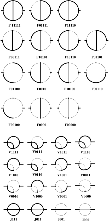
Figure 1: The F, V and J topologies. Bold and thin lines correspond to the mass and massless propagators, respectively.

The full set of two-loop self energy diagrams with one mass and external momentum on the same mass shell is given in Fig.1. We distinguish three basic topologies which in accordance with notations in Ref.[14] we call F, V and J prototypes with five, four and three lines, respectively. Our notation is given in Fig.2. The diagrams implemented in the package SHELL2 (F01101, F00110, V1110, V0011, V1000 in our notation) and those considered in detail in Refs.[18]-[20] (F00000, V0000, J001, J000) are not discussed here .

Figure 2: Notations used in present paper.

The general prototype involves arbitrary integer powers of the scalar denominators $c_{L}=k_{L}^{2}+m_{L}^{2}$ . Their powers $j_{L}$ are called indices of the lines. The mass-shell condition for the external momentum now is $p^{2}=-m^{2}$. Any scalar products of the momenta in the numerator arising from projection or expansion are reduced to powers of the scalar propagators (in case of V and J topologies the corresponding lines are added). Thus, the indices may sometimes become negative. Recurrence relations are derived via the integration-by-parts method [19] and applied to the massive case as in Ref.[22]. They allow to reduce all lines with negative indices to zero and the positive indices to one or zero. Further we use the shorthand notation $\{123\}$ of Ref. [23] to denote the relation for the triangle formed of lines $1$, $2$, and $3$:

$$\int\frac{d^{N}k}{c_{1}^{j_{1}}c_{2}^{j_{2}}c_{3}^{j_{3}}}\Big{(}N-2j_{1}-j_{2}-j_{3}+j_{1}\frac{2m_{1}^{2}}{c_{1}}+j_{2}\frac{m_{1}^{2}+m_{2}^{2}-m_{12}^{2}+c_{12}-c_{1}}{c_{2}}$$

$$+j_{3}\frac{m_{1}^{2}+m_{3}^{2}-m_{13}^{2}+c_{13}-c_{1}}{c_{3}}\Big{)}=0,$$

where a double index like $\{12\}$ refers to a line that starts at the point where lines $1$ and $2$ meet (see Fig.3). For an external line on the mass shell, the value of $c_{L}$ is equal to zero.

Figure 3: “Triangle” rule.

2.1 F-topology

To exclude the numerator (for example, $j_{1}<0,~{}~{}~{}c_{1}^{|j_{1}|}$ in the numerator) of F-type diagrams we use the following set of recurrence relations:

1. $j_{5}\neq 1$

   $$\{245\} \frac{j_{5}}{c_{5}}c_{1}=-\frac{j_{2}}{c_{2}}2m_{2}^{2}-\frac{j_{4}}{c_{4}}\left(m_{4}^{2}+m_{2}^{2}-m^{2}-c_{2}\right)$$

   $$-\frac{j_{5}}{c_{5}}\left(m_{5}^{2}+m_{2}^{2}-m_{1}^{2}-c_{2}\right)-N+2j_{2}+j_{4}+j_{5},$$

2. $j_{2}\neq 1$

   $$\{524\} \frac{j_{2}}{c_{2}}c_{1}=-\frac{j_{5}}{c_{5}}2m_{5}^{2}-\frac{j_{4}}{c_{4}}\left(m_{5}^{2}+m_{4}^{2}-m_{3}^{2}+c_{3}-c_{5}\right)$$

   $$-\frac{j_{2}}{c_{2}}\left(m_{5}^{2}+m_{2}^{2}-m_{1}^{2}-c_{5}\right)-N+2j_{5}+j_{4}+j_{2},$$

3. $j_{3}\neq 1$

   $$\{245\}+\{135\} \frac{j_{3}}{c_{3}}c_{1}=\frac{j_{3}}{c_{3}}\left(m_{3}^{2}+m_{1}^{2}-m^{2}\right)$$

   $$+\frac{j_{4}}{c_{4}}\left(m_{2}^{2}+m_{4}^{2}-m^{2}\right)$$

   $$-\frac{j_{4}}{c_{4}}c_{2}+\frac{j_{1}}{c_{1}}2m_{1}^{2}+\frac{j_{2}}{c_{2}}2m_{2}^{2}+\frac{j_{5}}{c_{5}}2m_{5}^{2}$$

   $$+2N-2j_{1}-2j_{2}-j_{3}-j_{4}-2j_{5},$$

4. $j_{2}=j_{3}=j_{5}=1$

   $$\{315\} N-2j_{3}-j_{1}-j_{5}=-\frac{j_{1}}{c_{1}}\left(m_{1}^{2}+m_{3}^{2}-m^{2}-c_{3}\right)$$

   $$-\frac{j_{5}}{c_{5}}\left(m_{3}^{2}+m_{5}^{2}-m_{4}^{2}+c_{4}-c_{3}\right)-\frac{j_{3}}{c_{3}}2m_{3}^{2},$$

where both sides of these relations are understood to be multiplied by
$\int\frac{d^{N}k_{1}d^{N}k_{2}}{c_{1}^{j_{1}}c_{2}^{j_{2}}c_{3}^{j_{3}}c_{4}^{j_{4}}c_{5}^{j_{5}}}.$ The relations for $(j_{2},j_{3},j_{4})<0$ are obtained from symmetry properties of the integral under consideration:

$$(j_{1},m_{1})\leftrightarrow(j_{3},m_{3}),~{}~{}~{}(j_{2},m_{2})\leftrightarrow(j_{4},m_{4}),$$

and

$$(j_{1},m_{1})\leftrightarrow(j_{2},m_{2}),~{}~{}~{}(j_{3},m_{3})\leftrightarrow(j_{4},m_{4}).$$

$c_{5}$ from the numerator can be eliminated by a general projection-operator method [19]. Using the decomposition

$$k_{1}k_{2}=A(k_{1},k_{2},p)+\frac{(k_{1}p)(k_{2}p)}{p^{2}},$$

where $A(k_{1},k_{2},p)=k_{1}^{\mu}\left(\delta_{\mu\nu}-\frac{p_{\mu}p_{\nu}}{p^{2}}\right)k_{2}^{\nu},$ and the property that odd powers of $A(k_{1},k_{2},p)$ drop out after integration and for even powers we have

$$\displaystyle\int{\rm d}^{N}k_{1}~{}{\rm d}^{N}k_{2}~{}f_{1}[k_{1},p]~{}f_{2}[k_{2},p]~{}A^{2n}(k_{1},k_{2},p)\,=$$

$$\displaystyle\mbox{$\,\displaystyle{\displaystyle\Gamma(n+\mbox{${1\over 2}$})\,\Gamma\big{[}\mbox{${1\over 2}$}(N-1)\big{]}\over\displaystyle\Gamma(\mbox{${1\over 2}$})\,\Gamma\big{[}n+\mbox{${1\over 2}$}(N-1)\big{]}}\,$}\prod_{j=1}^{2}\int{\rm d}^{N}k_{j}~{}f_{j}[k_{j},p]~{}A^{n}(k_{j},k_{j},p)\,,$$

it is possible to reduce the initial integral to a product of one-loop integrals.

Using the above relations, F-type integrals with arbitrary indices are reduced to F-type integrals with only positive indices or V-type integrals with arbitrary indices. For the former case a proper arrangement of recurrence relations in general reduces the sum of all indices by 1. These relations are given in appendix A. Only eight diagrams (F11111, F00111, F10101, F10110, F01100, F00101, F10100, F00001) with all indices equal to 1 form the basis for F-type diagrams.

2.2 V-topology

Consider now the V-type diagrams. The recurrence relations we use are $\{425\}$, $\{423\}$ and the following set:

$$\{530\} N-2j_{5}-j_{3}+\frac{j_{5}}{c_{5}}2m_{5}^{2}+\frac{j_{3}}{c_{3}}\left(m_{3}^{2}+m_{5}^{2}-m_{4}^{2}+c_{4}-c_{5}\right)=0,$$

$$\{350\} N-2j_{3}-j_{5}+\frac{j_{3}}{c_{3}}2m_{3}^{2}+\frac{j_{5}}{c_{5}}\left(m_{5}^{2}+m_{3}^{2}-m_{4}^{2}+c_{4}-c_{3}\right)=0,$$

$$\{B\} \frac{j_{5}}{c_{5}}\frac{\left(m_{4}^{2}-m_{2}^{2}+m^{2}+c_{2}-c_{4}\right)\left(m_{5}^{2}-m_{3}^{2}-m_{4}^{2}+c_{3}+c_{4}-c_{5}\right)}{2c_{6}}$$

$$+\frac{j_{2}}{c_{2}}2m^{2}-\left(\frac{j_{2}}{c_{2}}+\frac{j_{4}}{c_{4}}+\frac{j_{5}}{c_{5}}\right)\left(m_{4}^{2}-m_{2}^{2}+m^{2}+c_{2}-c_{4}\right)=0,$$

where $c_{6}=c_{4}-m_{4}^{2}$ (see Ref.[17]). If $m_{4}^{2}\neq 0$, the expression $\frac{1}{c_{4}c_{6}}$ can be simplified later by partial fraction decomposition. For all cases $(j_{2},j_{3},j_{5})<0$, except $j_{4}<0$, the initial diagram can be reduced to two-loop tadpole-like integrals by means of [6]:

$$\int d^{N}k_{2}\left(k_{2}p\right)^{2j}f(k_{2},k_{1})=\frac{(2j)!}{(j)!}\left(\frac{p^{2}}{4}\right)^{j}\frac{\Gamma\left(\frac{N}{2}\right)}{\Gamma\left(\frac{N}{2}+j\right)}\int d^{N}k_{2}(k_{2}^{2})^{j}f(k_{2},k_{1}).$$

For $j_{4}<0$ we write $c_{4}=\overline{c}_{4}+m_{4}^{2}$ and redefine $\overline{c}_{4}=c_{4}$, which allows to consider only the massless case. Then the following recurrence relations are needed:

1. $j_{5}\neq 1$

   $$\{350\} \frac{j_{5}}{c_{5}}c_{4}=\frac{j_{5}}{c_{5}}\left(c_{3}-m_{3}^{2}-m_{5}^{2}\right)-2\frac{j_{3}}{c_{3}}m_{3}^{2}-N+2j_{3}+j_{5},$$

2. $j_{3}\neq 1$

   $$\{530\} \frac{j_{3}}{c_{3}}c_{4}=\frac{j_{3}}{c_{3}}\left(c_{5}-m_{3}^{2}-m_{5}^{2}\right)-2\frac{j_{5}}{c_{5}}m_{5}^{2}-N+2j_{5}+j_{3},$$

3. $j_{2}\neq 1$

   $$\{425\}+\{350\} \frac{j_{2}}{c_{2}}c_{4}=\frac{j_{3}}{c_{3}}2m_{3}^{2}+\frac{j_{4}}{c_{4}}2m_{4}^{2}+\frac{j_{5}}{c_{5}}2m_{5}^{2}$$

   $$+\frac{j_{2}}{c_{2}}\left(m_{2}^{2}-m^{2}\right)+2N-j_{2}-2j_{3}-2j_{4}-2j_{5}.$$

4. $j_{2}=j_{3}=j_{5}=1$

   $$2B+2\{425\}+\{350\} 3N-4j_{2}-2j_{3}-2j_{4}-2j_{5}=-2m_{3}^{2}\frac{j_{3}}{c_{3}}-4m_{2}^{2}\frac{j_{2}}{c_{2}}$$

   $$+\frac{j_{5}}{c_{5}}\frac{c_{2}}{c_{4}}\left(c_{4}-c_{3}+m_{3}^{2}-m_{5}^{2}\right)+\frac{j_{5}}{c_{5}}\frac{c_{3}}{c_{4}}\left(m_{2}^{2}-m^{2}\right)$$

   $$+\left(j_{5}+2j_{4}\right)\frac{c_{2}+m^{2}-m_{2}^{2}}{c_{4}}+\frac{j_{5}}{c_{5}}\left(m^{2}-m_{2}^{2}-2m_{5}^{2}\right)$$

   $$+\frac{j_{5}}{c_{5}}\frac{\left(m_{3}^{2}-m_{5}^{2}\right)\left(m^{2}-m_{2}^{2}\right)}{c_{4}}.$$

The result of application of the above recurrence relations are V-type diagrams with only positive indices or J-type integrals with arbitrary indices. The full set of recurrence relations for the former case is given in appendix B. The complete set of basic integrals is just given by V1111 and V1001 with indices equal to 1.

2.3 J-topology

The integrals of this type are discussed in detail in Refs.[13, 14]. We only mention here, that to reduce the numerator the following recurrence relation, suggested by Tarasov [24], is needed:

$$(N+\nu_{1}+\nu_{2}\ -2)v(\nu_{1},\nu_{2})=p^{2}\{(\nu_{1}-1)k_{1}^{2}{\bf 1^{-}}\!+\nu_{2}(k_{1}k_{2}){\bf 2^{-}}\}{\bf 1^{-}}v(\nu_{1},\nu_{2}),$$

where $v(\nu_{1},\nu_{2})=\int d^{N}k_{1}d^{N}k_{2}f(k_{1},k_{2})(k_{1}p)^{\nu_{1}}(k_{2}p)^{\nu_{2}}$ and $f(k_{1},k_{2})$ is an arbitrary scalar function; $\nu_{1},\nu_{2}>0$ and ${\bf 1^{\pm}}v(\nu_{1},\nu_{2})\equiv v(\nu_{1}\pm 1,\nu_{2}),etc.$

The master integrals are the following: one prototype J111 with all indices equal to 1, and two integrals of J011-type: with indices 111 and 112, respectively.

2.4 Master-integrals

To obtain the finite part of two-loop physical results one needs to know the finite part of F-type integrals, V- and J-type integrals up to order $\varepsilon$, and one-loop integrals up to order $\varepsilon^{2}$. A detailed discussion of the calculation of master-integrals is given in [21]. Here me mention only, that the calculation of the $\varepsilon$ ($\varepsilon^{2}$) parts has been performed by the differential equation method [22]. The results are collected in Appendix C.

3 Use of the package

The package consists of a set of procedures for the calculation of all two-loop integrals, presented in Fig.1 (f11111.prc, $\cdots,$ on3.prc, on2.prc, etc), two-loop tadpoles (vl111.prc, vl011.prc, vl001.prc) and one-loop integrals (vl1.prc, on1.prc, ons11.prc), where “1”(“0”) in the name of the procedure stands for massive (massless) lines, respectively. on3 and on2 are two-loop integrals from the SHELL2 package. vl1 is the one-loop massive bubble. ons11 and on1 denote the one-loop self-energy on-shell integrals with two and one massive lines, respectively. The integration momenta in the package are denoted by K1 and K2 for two-loop integrals and by K1 for one-loop integrals, P is the external momentum. All scalar products in the initial diagram must be rewritten in terms of propagators:

$$k_{1}p = \frac{c_{1}-c_{3}+m_{3}^{2}-m_{1}^{2}-m^{2}}{2},$$

$$k_{2}p = \frac{c_{2}-c_{4}+m_{4}^{2}-m_{2}^{2}-m^{2}}{2},$$

$$k_{1}k_{2} = \frac{c_{1}+c_{2}-c_{5}+m_{5}^{2}-m_{1}^{2}-m_{2}^{2}}{2},$$

$$k_{1}^{2} = c_{1}-m_{1}^{2},$$

$$k_{2}^{2} = c_{2}-m_{2}^{2}.$$

To specify the type of two- (one-) loop diagrams, the products of scalar propagators must be substituted by the proper functions of F-, V-, J- and ON-type with arguments denoting the indices and a symbol for the mass shell.

To work with fractions of N-dimensional numbers, two functions, SS and NN (originating from the package “LEO” [23] ) are used:

$$NN(a,j)=\left(N+a\right)^{j},~{}~{}~{}~{}~{}j>0,$$

and

$$SS(a,j)=\frac{1}{\left(N+a\right)^{j}},~{}~{}~{}~{}~{}j>0.$$

After application of each recurrence relation the procedure “ration” for the simplification of products of SS’s and NN’s must be called. The procedure “finitem” substitutes the values of master integrals and performs the expansion of the functions NN and SS in $\varepsilon$.

The integration procedure starts with F-type integrals. We apply the recurrence relations given explicitly in appendix A. After applying them several times, the integrand is reduced to the master integrals or to new, more simple, integrals like V-type, e.g. Then we apply several times the recurrence relations of Appendix B for the V-types. One needs to call all procedures step by step to reduce the initial diagram to the set of master integrals. The recommended sequence for calling the procedures is the following one:

#call f11111{’TIMES’}
#call f01111{’TIMES’}
#call f11110{’TIMES’}
#call f00111{’TIMES’}
#call f10101{’TIMES’}
#call f10110{’TIMES’}
#call f01100{’TIMES’}
#call f00101{’TIMES’}
#call f10100{’TIMES’}
#call f00100{’TIMES’}
#call f00001{’TIMES’}
#call f00000{’TIMES’}
#call v1111{’TIMES’}
#call v0111{’TIMES’}
#call v1011{’TIMES’}
#call v1010{’TIMES’}
#call v0110{’TIMES’}
#call v1001{’TIMES’}
#call v0010{’TIMES’}
#call v0001{’TIMES’}
#call v0000{’TIMES’}
#call j011{’TIMES’}
#call on3{’TIMES’}
#call on2{’TIMES’}
#call vl111{’TIMES’}
#call vl011{’TIMES’}
#call vl001{’TIMES’}
#call on1{2*’TIMES’}
#call ons11{2*’TIMES’}
#call vl00{’TIMES’}
#call vl1{2*’TIMES’}

All programs of the package are realized with the help of FORM procedure facilities. To perform the integration, one needs to call the procedures with the name of the corresponding prototypes and one argument which determines how often the recurrence relations are to be called. This number depends on the complexity of the calculated diagram. In most cases it is equal to the sum of indices of the integrand.

Figure 4:

Let us consider as an example, the physical diagram shown in Fig.4 in more detail. The FORM input is created automatically by DIANA [25]. For two-loop self-energy diagrams DIANA generates all necessary information, e.g. identifying symbols for the particles of the diagram and their masses , distribution of integration momenta, Feynman rules (linear/nonlinear gauges), number of fermion loops, symmetry factors, etc. To calculate the transverse part it is sufficient to make the following substitutions:

multiply, (d_(mu,nu)-p(mu)*p(nu)/p.p)*SS(-1,1);
.sort
id k1.p = (k1.k1-c3)/2;
id k2.p = (k2.k2-c4+mmZ-mmW)/2;
id k1.k2 = -(c5 - k1.k1 - k2.k2 - mmW)/2;
id k1.k1 = c1 - mmZ;
id k2.k2 = c2 - mmW;
id p.p^j? = (-mmW)^j;
.sort
id mmZ^j? = mmW^j;
id 1/c1^j1?/c2^j2?/c3^j3?/c4^j4?/c5^j5? = F11111(j1,j2,j3,j4,j5,mmW),

where we have explicitly set $m_{W}^{2}=m_{Z}^{2}$ Calling the above routines (not all of them are needed in this special case) yields the result

$${\it Example1}=m_{W}^{2}{\bf F11111}(1,1,1,1,1,m_{W}^{2})\Biggl{(}33-\frac{11}{N-1}\Biggr{)}$$

$$+{\bf V1111}(1,1,1,1,m_{W}^{2})\Biggl{(}-42+\frac{2}{N-1}+\frac{27}{4(N-1)^{2}}\Biggr{)}$$

$$+\frac{{\bf J111}(1,1,1,m_{W}^{2})}{m_{W}^{2}}\Biggl{(}\frac{4}{3}-\frac{26}{3(N-1)}+\frac{17}{4(N-1)^{2}}\Biggr{)}$$

$$+\frac{{\bf VL111}(1,1,1,m_{W}^{2})}{m_{W}^{2}}\Biggl{(}20-\frac{5}{2(N-1)}-\frac{9}{4(N-1)^{2}}\Biggr{)}$$

$$+\left[{\bf ONS11}(1,1,m_{W}^{2})\right]^{2}\Biggl{(}\frac{5}{(N-1)}-\frac{21}{2}\Biggr{)}$$

$$+{\bf ONS11}(1,1,m_{W}^{2})\Biggl{(}-\frac{17}{3(N-4)}-\frac{1}{(N-2)}+\frac{20}{3(N-1)}-\frac{6}{(N-1)^{2}}\Biggr{)}$$

$$+\Biggl{(}\frac{64}{3(N-4)}-\frac{24}{(N-4)^{2}}-\frac{32}{(N-2)}-\frac{8}{(N-2)^{2}}+\frac{32}{3(N-1)}\Biggr{)},$$

where the overall factor is $\frac{g^{4}m_{W}^{2}}{(16\pi^{2})^{2}}$. After calling “finitem” we have:

$${\it Example1} = -\frac{1417}{24\epsilon^{2}}-\frac{1}{\varepsilon}\Biggl{(}\frac{10375}{48}-\frac{665}{12}\frac{\pi}{\sqrt{3}}\Biggr{)}-\frac{21187}{32}+\frac{21}{8}\zeta(2)-\frac{88}{3}\zeta(3)$$

$$+\frac{4007}{18}\frac{\pi}{\sqrt{3}}-\frac{665}{12}\frac{\pi}{\sqrt{3}}\ln 3+\frac{16449}{16}S_{2}+132\frac{\pi}{\sqrt{3}}S_{2}$$

$$\approx-\frac{59.0}{\varepsilon^{2}}-\frac{115.6}{\varepsilon}-69.6.$$

So far we have considered only the case of merely one non-zero mass. Of course it is obvious that as further application of our package we use it for the expansion of diagrams in terms of mass differences. In general a ‘standard’ expansion of the scalar propagators in terms of the mass difference, i.e. in the above case in terms of $m_{W}^{2}-m_{Z}^{2}$, yields as expansion coefficients again integrals, which can be handled by our package. In order to demonstrate this possibility, we extend the calculation of the diagram in Fig.4 up to the second order in $\Delta\equiv 1-m_{W}^{2}/m_{Z}^{2}=\sin^{2}\theta_{W}$ with the result

$${\it Example1}=\frac{1}{\varepsilon^{2}}\Biggl{(}-\frac{1417}{24}+\frac{667}{8}\Delta-\frac{95}{4}\Delta^{2}\Biggr{)}$$

$$-\frac{1}{\varepsilon}\Biggl{(}\frac{10375}{48}-\frac{24197}{72}\Delta+\frac{17957}{144}\Delta^{2}\Biggr{)}+\frac{1}{\varepsilon}\frac{\pi}{\sqrt{3}}\Biggl{(}\frac{665}{12}-\frac{137}{3}\Delta-\frac{635}{72}\Delta^{2}\Biggr{)}$$

$$+\frac{\pi}{\sqrt{3}}\Biggl{(}\frac{4007}{18}-\frac{21881}{72}\Delta+\frac{45067}{432}\Delta^{2}\Biggr{)}-\frac{\pi}{\sqrt{3}}\ln 3\Biggl{(}\frac{665}{12}-\frac{137}{3}\Delta-\frac{635}{72}\Delta^{2}\Biggr{)}$$

$$+S_{2}\Biggl{(}\frac{16449}{16}-\frac{7461}{8}\Delta+\frac{2195}{32}\Delta^{2}\Biggr{)}+\frac{\pi}{\sqrt{3}}S_{2}\Biggl{(}132-\frac{351}{4}\Delta+\frac{699}{4}\Delta^{2}\Biggr{)}$$

$$-\Biggl{(}\frac{21187}{32}-\frac{216049}{216}\Delta+\frac{403637}{864}\Delta^{2}\Biggr{)}+\zeta(2)\Biggl{(}\frac{21}{8}-\frac{1477}{36}\Delta+\frac{23179}{432}\Delta^{2}\Biggr{)}$$

$$-\zeta(3)\Biggl{(}\frac{88}{3}-\frac{39}{2}\Delta+\frac{233}{6}\Delta^{2}\Biggr{)}\approx\frac{1}{\varepsilon^{2}}\left(-59.0+83.4\Delta-23.8\Delta^{2}\right)$$

$$+\frac{1}{\varepsilon}\left(-115.6+253.2\Delta-140.7\Delta^{2}\right)-69.6+211.6\Delta-118.4\Delta^{2}.$$

With the numerical value $\Delta\simeq 0.23$, we see that the convergence in $\Delta$ of the above series in the three contributions is quite good and it can be expected that it will even improve due to ‘gauge cancellations’ if a complete gauge invariant subset of diagrams is taken into account.

4 Conclusion

The presented package has been developed for the calculation of two-loop self energy diagrams with only one non-zero mass. All mass combinations of the Standard Model with heavy masses are included. In this sense it is an extension of the existing package SHELL2, which takes into account only diagrams occurring in QED and QCD. We have also shown that this package can be used for the case of different masses in the SM by expanding in terms of mass differences. Thus we have provided a program for the evaluation of at least a large class of on-shell two-loop self energy diagrams in the SM. The time of calculation of one diagram, depending of course on the order of expansion in the mass differences, is not very large in general.

Acknowledgments We are grateful to A. Davydychev, A. V. Kotikov, O. V. Tarasov, M. Tentyukov and O. Veretin for useful comments. M.K. ’s research has been supported by the DFG project FL241/4-1 and in part by RFBR $\#$98-02-16923.

Appendix

Appendix A The set of recurrence relations for F-type integrals

The full set of recurrence relations valid for arbitrary masses and momenta is given in Ref.[26]. Here we present some rearrangement of these relations which allows to reduce the positive indices of the on-shell diagrams with one mass to 0 or 1.

1. F11111

   $$4m^{2}\frac{j_{1}}{c_{1}} = \frac{j_{1}}{c_{1}}\left(c_{2}-c_{3}-c_{5}\right)+\frac{j_{3}}{c_{3}}\left(3c_{1}+c_{4}-c_{5}\right)$$

   $$+\frac{j_{5}}{c_{5}}\left(3c_{1}-3c_{2}+c_{4}-c_{3}\right)-N+4j_{1},$$

   $$4m^{2}\frac{j_{5}}{c_{5}} = \frac{j_{1}}{c_{1}}\left(3c_{5}-3c_{2}-c_{3}\right)+\frac{j_{3}}{c_{3}}\left(3c_{5}-3c_{4}-c_{1}\right)$$

   $$+\frac{j_{5}}{c_{5}}\left(c_{4}-c_{3}+c_{2}-c_{1}\right)-N+4j_{5}.$$

2. F01111

   $$N-2j_{1}-j_{3}-j_{5} = \frac{j_{5}}{c_{5}}\left(c_{1}-c_{2}\right)+\frac{j_{3}}{c_{3}}c_{1}.$$

3. F11110

   $$N-2j_{5}-j_{1}-j_{3} = \frac{j_{1}}{c_{1}}\left(c_{5}-c_{2}\right)+\frac{j_{3}}{c_{3}}\left(c_{5}-c_{4}\right).$$

4. F00111

   $$2m^{2}\frac{j_{1}}{c_{1}} = \frac{j_{1}}{c_{1}}\left(2c_{5}-2c_{2}-c_{3}\right)+\frac{j_{3}}{c_{3}}\left(2c_{5}-2c_{4}-3c_{1}\right)$$

   $$+\frac{j_{5}}{c_{5}}\left(3c_{2}-3c_{1}+c_{4}-c_{3}\right)+2N-3j_{3}-5j_{1},$$

   $$2m^{2}\frac{j_{3}}{c_{3}} = \frac{j_{1}}{c_{1}}c_{3}-\frac{j_{3}}{c_{3}}c_{1}+\frac{j_{5}}{c_{5}}\left(c_{2}-c_{1}+c_{3}-c_{4}\right)+j_{3}-j_{1},$$

   $$2m^{2}\frac{j_{5}}{c_{5}} = \frac{j_{3}}{c_{3}}c_{1}+\frac{j_{4}}{c_{4}}c_{2}-2N+2j_{1}+2j_{2}+2j_{5}+j_{3}+j_{4}.$$

5. F10101

   $$m^{2}\frac{j_{1}}{c_{1}} = \frac{j_{3}}{c_{3}}\left(c_{5}-c_{4}\right)+\frac{j_{1}}{c_{1}}\left(c_{5}-c_{2}-c_{3}\right)$$

   $$+\frac{j_{5}}{c_{5}}\left(c_{4}-c_{3}\right)+j_{5}-j_{3},$$

   $$m^{2}\frac{j_{2}}{c_{2}} = \frac{j_{5}}{c_{5}}\left(c_{3}-c_{4}\right)-\frac{j_{2}}{c_{2}}c_{4}+N-2j_{4}-j_{2}-j_{5},$$

   $$2m^{2}\frac{j_{5}}{c_{5}} = \frac{j_{2}}{c_{2}}\left(c_{5}-c_{1}\right)+\frac{j_{4}}{c_{4}}\left(c_{5}-c_{3}\right)-N+2j_{5}+j_{2}+j_{4}.$$

6. F10110

   $$2m^{2}\frac{j_{4}}{c_{4}} = \frac{j_{2}}{c_{2}}c_{4}-\frac{j_{5}}{c_{5}}\left(c_{3}-c_{4}\right)-N+2j_{4}+j_{2}+j_{5},$$

   $$m^{2}\frac{j_{2}}{c_{2}} = \frac{j_{2}}{c_{2}}\left(c_{1}-c_{5}\right)+\frac{j_{4}}{c_{4}}\left(c_{3}-c_{5}\right)+N-2j_{5}-j_{2}-j_{4},$$

   $$m^{2}\frac{j_{5}}{c_{5}} = \frac{j_{5}}{c_{5}}\left(c_{1}-c_{2}\right)-\frac{j_{4}}{c_{4}}c_{2}+N-2j_{2}-j_{4}-j_{5},$$

   $$m^{2}\frac{j_{1}}{c_{1}} = \frac{j_{1}}{c_{1}}\left(c_{5}-c_{2}\right)+\frac{j_{3}}{c_{3}}\left(c_{5}-c_{4}\right)-N+2j_{5}+j_{1}+j_{3},$$

   $$2m^{2}\frac{j_{3}}{c_{3}} = \frac{j_{3}}{c_{3}}\left(c_{4}-c_{5}\right)+\frac{j_{5}}{c_{5}}\left(c_{3}-c_{4}\right)+\frac{j_{1}}{c_{1}}\left(c_{2}+c_{3}-c_{5}\right)+j_{3}-j_{5}$$

7. F01100

   $$2m^{2}\frac{j_{1}}{c_{1}} = \frac{j_{1}}{c_{1}}\left(2c_{2}-2c_{5}+c_{3}\right)+\frac{j_{3}}{c_{3}}\left(2c_{4}-2c_{5}+c_{1}\right)$$

   $$+\frac{j_{5}}{c_{5}}\left(c_{1}-c_{2}+c_{3}-c_{4}\right)+j_{1}+j_{3}-2j_{5},$$

   $$2m^{2}\frac{j_{2}}{c_{2}} = \frac{j_{2}}{c_{2}}c_{4}+\frac{j_{4}}{c_{4}}c_{2}+\frac{j_{5}}{c_{5}}\left(c_{2}-c_{1}+c_{4}-c_{3}\right)$$

   $$-2N+2j_{5}+3j_{2}+3j_{4},$$

   $$m^{2}\frac{j_{5}}{c_{5}} = \frac{j_{5}}{c_{5}}\left(c_{2}-c_{1}\right)-\frac{j_{3}}{c_{3}}c_{1}+N-2j_{1}-j_{3}-j_{5}.$$

8. F00101

   $$m^{2}\frac{j_{5}}{c_{5}} = \frac{j_{5}}{c_{5}}\left(c_{1}-c_{2}\right)+\frac{j_{3}}{c_{3}}c_{1}-N+2j_{1}+j_{3}+j_{5},$$

   $$m^{2}\frac{j_{2}}{c_{2}} = \frac{j_{5}}{c_{5}}\left(c_{3}-c_{4}\right)-\frac{j_{2}}{c_{2}}c_{4}+N-2j_{4}-j_{2}-j_{5},$$

   $$m^{2}\frac{j_{4}}{c_{4}} = 2\frac{j_{5}}{c_{5}}\left(c_{1}-c_{2}\right)-\frac{j_{4}}{c_{4}}c_{2}+\frac{j_{3}}{c_{3}}c_{1}+2j_{1}-2j_{2}+j_{3}-j_{4},$$

   $$2m^{2}\frac{j_{3}}{c_{3}} = \frac{j_{1}}{c_{1}}c_{3}-2\frac{j_{3}}{c_{3}}c_{1}+\frac{j_{5}}{c_{5}}\left(2c_{2}-2c_{1}+c_{3}-c_{4}\right)+N-3j_{1}-j_{5},$$

   $$m^{2}\frac{j_{1}}{c_{1}} = \frac{j_{1}}{c_{1}}\left(c_{5}-c_{2}-c_{3}\right)+\frac{j_{3}}{c_{3}}\left(c_{5}-c_{4}\right)+\frac{j_{5}}{c_{5}}\left(c_{4}-c_{3}\right)+j_{5}-j_{3}.$$

9. F10100

   $$2m^{2}\frac{j_{1}}{c_{1}} = \frac{j_{1}}{c_{1}}\left(c_{5}-c_{2}-c_{3}\right)+\frac{j_{3}}{c_{3}}\left(c_{1}-c_{4}+c_{5}\right)$$

   $$+\frac{j_{5}}{c_{5}}\left(c_{1}-c_{2}-c_{3}+c_{4}\right)-N+2j_{1}+2j_{5},$$

   $$2m^{2}\frac{j_{2}}{c_{2}} = \frac{j_{2}}{c_{2}}\left(c_{1}-c_{4}-c_{5}\right)+\frac{j_{4}}{c_{4}}\left(c_{2}+c_{3}-c_{5}\right)+\frac{j_{5}}{c_{5}}\left(c_{2}-c_{1}+c_{3}-c_{4}\right)+N-2j_{4}-j_{5},$$

   $$2m^{2}\frac{j_{5}}{c_{5}} = \frac{j_{1}}{c_{1}}\left(3c_{2}+c_{3}-3c_{5}\right)+\frac{j_{3}}{c_{3}}\left(c_{1}+3c_{4}-3c_{5}\right)$$

   $$+\frac{j_{5}}{c_{5}}\left(c_{1}-c_{2}+c_{3}-c_{4}\right)+N-4j_{5}.$$

10. F00100

    $$N-2j_{1}-j_{3}-j_{5} = \frac{j_{5}}{c_{5}}\left(c_{1}-c_{2}\right)+\frac{j_{3}}{c_{3}}c_{1}.$$

11. F00001

    $$4m^{2}\frac{j_{1}}{c_{1}} = \frac{j_{1}}{c_{1}}\left(c_{5}-c_{2}-3c_{3}\right)+\frac{j_{3}}{c_{3}}\left(c_{1}-c_{4}+c_{5}\right)$$

    $$+\frac{j_{5}}{c_{5}}\left(c_{1}-c_{2}-3c_{3}+3c_{4}\right)+N-4j_{3},$$

    $$4m^{2}\frac{j_{5}}{c_{5}} = \frac{j_{1}}{c_{1}}\left(c_{5}+c_{3}-c_{2}\right)+\frac{j_{3}}{c_{3}}\left(c_{5}+c_{1}-c_{4}\right)$$

    $$+\frac{j_{5}}{c_{5}}\left(c_{1}-c_{2}+c_{3}-c_{4}\right)-3N+4j_{1}+4j_{3}+4j_{5}.$$

Appendix B The set of recurrence relations for V-type integrals

The full set of recurrence relations for the V-type integrals is also given in Ref.[26]. Here we give our rearrangement of these relations which again allows to reduce positive indices of the on-shell diagrams with one mass to 0 or 1.

1. V1111

   $$3m^{2}\frac{j_{3}}{c_{3}} = \frac{j_{3}}{c_{3}}\left(c_{4}-c_{5}\right)+2\frac{j_{5}}{c_{5}}\left(c_{3}-c_{4}\right)-N+3j_{3},$$

   $$3m^{2}\frac{j_{2}}{c_{2}} = j_{5}\left(\frac{c_{2}}{c_{6}}-\frac{c_{2}c_{3}}{c_{5}c_{6}}\right)+2\frac{j_{4}}{c_{4}}c_{2}+\frac{j_{5}}{c_{5}}c_{2}-\frac{j_{2}}{c_{2}}c_{4}-N+3j_{2},$$

   $$3m^{2}\frac{j_{4}}{c_{4}} = \frac{j_{5}}{2}\left(\frac{c_{2}c_{3}}{c_{5}c_{6}}-\frac{c_{2}}{c_{6}}\right)+2\frac{j_{2}}{c_{2}}c_{4}-\frac{j_{4}}{c_{4}}c_{2}+\frac{j_{3}}{c_{3}}\left(c_{4}-c_{5}\right)$$

   $$+\frac{j_{5}}{2}\frac{2c_{4}-2c_{3}-c_{2}}{c_{5}}-\frac{N}{2}+3j_{4}.$$

2. V0111

   $$3m^{2}\frac{j_{3}}{c_{3}} = \frac{j_{3}}{c_{3}}\left(c_{4}-c_{5}\right)+2\frac{j_{5}}{c_{5}}\left(c_{3}-c_{4}\right)-N+3j_{3},$$

   $$2m^{2}\frac{j_{4}}{c_{4}} = \frac{2}{3}\frac{j_{3}}{c_{3}}\left(c_{4}-c_{5}\right)+\frac{2}{3}\frac{j_{5}}{c_{5}}\left(c_{4}-c_{3}\right)+\frac{j_{2}}{c_{2}}c_{4}$$

   $$-\frac{2}{3}N+2j_{4}+j_{2},$$

   $$2\left(N-2j_{2}-j_{4}\right) = \frac{j_{5}}{c_{5}}\left(c_{2}+c_{4}\right)+2\frac{j_{4}}{c_{4}}c_{2}+j_{5}\frac{c_{5}-c_{3}}{c_{5}}\frac{c_{2}+c_{4}}{c_{6}}.$$

3. V1011

   $$2m^{2}\frac{j_{3}}{c_{3}} = \frac{j_{5}}{c_{5}}\left(c_{3}-c_{4}\right)-N+2j_{3}+j_{5},$$

   $$\left(N-2j_{5}-j_{3}\right) = \frac{j_{3}}{c_{3}}\left(c_{5}-c_{4}\right).$$

4. V1010

   $$2m^{2}\frac{j_{3}}{c_{3}} = \frac{j_{2}}{c_{2}}c_{4}-2N+j_{2}+2j_{3}+2j_{4}+2j_{5},$$

   $$m^{2}\frac{j_{5}}{c_{5}} = \frac{j_{5}}{c_{5}}\left(c_{3}-c_{4}\right)-\frac{j_{2}}{c_{2}}c_{4}+N-2j_{4}-j_{2}-j_{5},$$

   $$4m^{2}\frac{j_{2}}{c_{2}} = m^{2}\frac{j_{5}}{c_{5}}\frac{c_{2}}{c_{4}}-\frac{j_{2}}{c_{2}}c_{4}+\left(j_{5}+2j_{4}\right)\frac{c_{2}}{c_{4}}$$

   $$-\frac{j_{5}}{c_{5}}\frac{c_{2}}{c_{4}}\left(c_{3}-c_{4}\right)-N+3j_{2},$$

   $$4\frac{m^{2}}{c_{4}}\left(j_{2}+2j_{4}\right) = -m^{2}\frac{j_{5}}{c_{5}}\frac{c_{2}}{c_{4}}+\frac{j_{2}}{c_{2}}\left(4c_{3}-3c_{4}-4c_{5}\right)-\left(j_{5}+2j_{4}\right)\frac{c_{2}}{c_{4}}$$

   $$+4\left(j_{2}+2j_{4}\right)\frac{c_{3}-c_{5}}{c_{4}}+\frac{j_{5}}{c_{5}}\frac{c_{2}}{c_{4}}\left(c_{3}-c_{4}\right)$$

   $$+9N-16j_{5}-8j_{4}-7j_{2},$$

   $$2j_{4}+j_{2}-2j_{5} = 2\frac{j_{3}}{c_{3}}\left(c_{5}-c_{4}\right)-\frac{j_{2}}{c_{2}}c_{4}.$$

5. V0110

   $$m^{2}\frac{j_{2}}{c_{2}} = \frac{j_{5}}{c_{5}}\left(c_{3}-c_{4}\right)-\frac{j_{2}}{c_{2}}c_{4}+N-2j_{4}-j_{2}-j_{5},$$

   $$4m^{2}\frac{j_{5}}{c_{5}} = m^{2}\frac{j_{2}}{c_{2}}\frac{c_{5}-c_{3}}{c_{4}}+\frac{j_{2}}{c_{2}}\left(c_{5}-c_{3}\right)+\frac{j_{5}}{c_{5}}\left(c_{3}-c_{4}\right)$$

   $$+\left(j_{2}+2j_{4}\right)\frac{c_{5}-c_{3}}{c_{4}}-N+3j_{5},$$

   $$4\frac{m^{2}}{c_{4}}\left(j_{5}+2j_{4}\right) = 4m^{2}\frac{j_{5}}{c_{5}}\frac{c_{3}}{c_{4}}+m^{2}\frac{j_{2}}{c_{2}}\frac{c_{3}-c_{5}}{c_{4}}+\frac{j_{2}}{c_{2}}\left(c_{3}-c_{5}\right)-4j_{5}\frac{c_{2}}{c_{4}}$$

   $$+j_{2}\frac{c_{3}-c_{5}}{c_{4}}-2\frac{j_{4}}{c_{4}}\left(4c_{2}-c_{3}+c_{5}\right)$$

   $$+\frac{j_{5}}{c_{5}}\left(4\frac{c_{2}c_{3}}{c_{4}}-4c_{2}+3c_{3}-3c_{4}\right)$$

   $$+9N-16j_{2}-8j_{4}-7j_{5}.$$

6. V1001

   $$\frac{j_{3}}{c_{3}} = -\frac{\left(N-2j_{3}-2j_{5}\right)\left(N-j_{3}-j_{5}-1\right)}{\left(N-2j_{3}-2\right)c_{6}},$$

   $$3m^{2}\frac{j_{4}}{c_{4}} = 2\frac{j_{2}}{c_{2}}c_{4}-\left(\frac{j_{4}}{c_{4}}+\frac{j_{6}}{c_{6}}\right)c_{2}-N+3j_{4}+3j_{6},$$

   $$3m^{2}\frac{j_{2}}{c_{2}} = 2\left(\frac{j_{4}}{c_{4}}+\frac{j_{6}}{c_{6}}\right)c_{2}-\frac{j_{2}}{c_{2}}c_{4}-N+3j_{2}.$$

7. V0010

   $$m^{2}\frac{j_{3}}{c_{3}} = \frac{j_{3}}{c_{3}}\left(c_{5}-c_{4}\right)-N+2j_{5}+j_{3},$$

   $$m^{2}\frac{j_{5}}{c_{5}} = 2\frac{j_{3}}{c_{3}}\left(c_{4}-c_{5}\right)+\frac{j_{5}}{c_{5}}\left(c_{3}-c_{4}\right)+N-3j_{5},$$

   $$m^{2}\frac{j_{2}}{c_{2}} = 2\frac{j_{3}}{c_{3}}\left(c_{5}-c_{4}\right)-\frac{j_{2}}{c_{2}}c_{4}+2j_{5}-2j_{4}-j_{2},$$

   $$\frac{m^{2}}{c_{4}}\left(N+2j_{4}-2j_{5}\right) = 2m^{2}\frac{j_{3}}{c_{3}}\frac{c_{5}}{c_{4}}-\left(2j_{4}+j_{5}\right)\frac{c_{2}}{c_{4}}+\frac{j_{5}}{c_{5}}\frac{c_{2}}{c_{4}}\left(c_{3}-c_{4}\right)$$

   $$-m^{2}\frac{j_{5}}{c_{5}}\frac{c_{2}}{c_{4}}+3N-4j_{2}-2j_{3}-2j_{4}-2j_{5}.$$

8. V0001

   $$\frac{j_{3}}{c_{3}} = -\frac{\left(N-2j_{3}-2j_{5}\right)\left(N-j_{3}-j_{5}-1\right)}{\left(N-2j_{3}-2\right)c_{6}},$$

   $$N-2j_{2}-j_{4} = \frac{j_{4}}{c_{4}}c_{2}-\left(\frac{N}{2}-2-j_{6}\right)\frac{c_{2}+c_{4}}{c_{6}}.$$

Appendix C Analytical results

For completeness, we present here the analytical results for all two-loop integrals shown in Fig.1

$${\bf F11111}(1,1,1,1,1,m) = -\zeta(3)+\frac{9}{2}\frac{\pi}{\sqrt{3}}S_{2}+{\cal O}(\varepsilon),$$

$${\bf F01111}(1,1,1,1,1,m) = \frac{4}{3}\zeta(2)\ln 3-\frac{5}{3}\zeta(3)+3\frac{\pi}{\sqrt{3}}S_{2}+{\cal O}(\varepsilon),$$

$${\bf F11110}(1,1,1,1,1,m) = -\frac{4}{3}\zeta(2)\ln 3+\frac{2}{3}\zeta(3)+6\frac{\pi}{\sqrt{3}}S_{2}+{\cal O}(\varepsilon),$$

$${\bf F00111}(1,1,1,1,1,m) = 9\frac{\pi}{\sqrt{3}}S_{2}+{\cal O}(\varepsilon),$$

$${\bf F10101}(1,1,1,1,1,m) = -4\zeta(3)+\frac{27}{2}\frac{\pi}{\sqrt{3}}S_{2}+i\frac{\pi}{3}\zeta(2)+{\cal O}(\varepsilon),$$

$${\bf F10110}(1,1,1,1,1,m) = -\zeta(3)+9\frac{\pi}{\sqrt{3}}S_{2}+{\cal O}(\varepsilon),$$

$${\bf F01101}(1,1,1,1,1,m) = 6\zeta(2)\ln 2-\frac{3}{2}\zeta(3)+{\cal O}(\varepsilon),$$

$${\bf F01100}(1,1,1,1,1,m) = \frac{27}{2}\frac{\pi}{\sqrt{3}}S_{2}+i\pi\zeta(2)+{\cal O}(\varepsilon),$$

$${\bf F00101}(1,1,1,1,1,m) = -3\zeta(3)+\frac{27}{2}\frac{\pi}{\sqrt{3}}S_{2}+i\pi\zeta(2)+{\cal O}(\varepsilon),$$

$${\bf F10100}(1,1,1,1,1,m) = -2\zeta(3)+9\frac{\pi}{\sqrt{3}}S_{2}+i\frac{2}{3}\pi\zeta(2)+{\cal O}(\varepsilon),$$

$${\bf F00110}(1,1,1,1,1,m) = -\frac{\zeta(2)}{\varepsilon}-2\zeta(2)-2\zeta(3)+{\cal O}(\varepsilon),$$

$${\bf F00100}(1,1,1,1,1,m) = -3\zeta(3)-2i\pi\zeta(2)+{\cal O}(\varepsilon),$$

$${\bf F00001}(1,1,1,1,1,m) = -3\zeta(3)+i\pi\zeta(2)+{\cal O}(\varepsilon),$$

$${\bf F00000}(1,1,1,1,1,m) = -6\zeta(3)+{\cal O}(\varepsilon),$$

where

$${\bf F}\{{\cal ABIJK}\}(a,b,i,j,k,m) \equiv m^{2}K^{-2}\int d^{N}k_{1}d^{N}k_{2}$$

$$P^{(a)}(k_{1},{\cal A}m)P^{(b)}(k_{2},{\cal B}m)$$

$$P^{(i)}(k_{1}-p,{\cal I}m)P^{(j)}(k_{2}-p,{\cal J}m)$$

$$\left.P^{(k)}(k_{1}-k_{2},{\cal K}m)\right|_{p^{2}=-m^{2}},$$

and

$$K=\frac{\Gamma(1+\varepsilon)}{\left(4\pi\right)^{\frac{N}{2}}\left(m^{2}\right)^{\varepsilon}},~{}~{}~{}P^{(l)}(k,m)\equiv\frac{1}{(k^{2}+m^{2})^{l}},$$

and where the normalization factor $1/(2\pi)^{N}$ for each loop is assumed; ${\cal A,B,I,J,K}=0,1$ and

$$S_{2}=\frac{4}{9\sqrt{3}}Cl_{2}\left(\frac{\pi}{3}\right)=0.2604341376\cdots.$$

$${\bf V1111}(1,1,1,1,m)=\frac{1}{2\varepsilon^{2}}+\frac{1}{\varepsilon}\left(\frac{5}{2}-\frac{\pi}{\sqrt{3}}\right)+\frac{19}{2}-\frac{\zeta(2)}{2}-4\frac{\pi}{\sqrt{3}}-\frac{63}{4}S_{2}$$

$$+\frac{\pi}{\sqrt{3}}\ln 3+\varepsilon\Biggl{\{}\frac{65}{2}-6\zeta(2)-\frac{9}{2}\zeta(3)-12\frac{\pi}{\sqrt{3}}-63S_{2}+4\zeta(2)\ln 3+9S_{2}\frac{\pi}{\sqrt{3}}$$

$$+\frac{63}{4}S_{2}\ln 3+4\frac{\pi}{\sqrt{3}}\ln 3-\frac{1}{2}\frac{\pi}{\sqrt{3}}\ln^{2}3-\frac{9}{2}\frac{\pi}{\sqrt{3}}\zeta(2)-\frac{21}{2}\frac{Ls_{3}\left(\frac{2\pi}{3}\right)}{\sqrt{3}}\Biggr{\}}+{\cal O}(\varepsilon^{2}),$$

$${\bf V0111}(1,1,1,1,m)=\frac{1}{2\varepsilon^{2}}+\frac{5}{2\varepsilon}+\frac{19}{2}-\frac{2}{3}\zeta(2)-\frac{\pi}{\sqrt{3}}-\frac{27}{2}S_{2}$$

$$+\varepsilon\Biggl{\{}\frac{65}{2}-\frac{8}{3}\zeta(2)+\frac{2}{3}\zeta(3)-7\frac{\pi}{\sqrt{3}}-\frac{135}{2}S_{2}+\frac{27}{2}S_{2}\ln 3-3\frac{\pi}{\sqrt{3}}\zeta(2)$$

$$+3\frac{\pi}{\sqrt{3}}\ln 3-9\frac{Ls_{3}\left(\frac{2\pi}{3}\right)}{\sqrt{3}}\Biggr{\}}+{\cal O}(\varepsilon^{2}),$$

$${\bf V1011}(1,1,1,1,m)=\frac{1}{2\varepsilon^{2}}+\frac{1}{\varepsilon}\left(\frac{5}{2}-\frac{\pi}{\sqrt{3}}\right)+\frac{19}{2}+\frac{\zeta(2)}{3}-5\frac{\pi}{\sqrt{3}}-9S_{2}$$

$$+\frac{\pi}{\sqrt{3}}\ln 3+\varepsilon\Biggl{\{}\frac{65}{2}+\frac{4}{3}\zeta(2)-\frac{\zeta(3)}{3}-19\frac{\pi}{\sqrt{3}}-\frac{99}{2}S_{2}+9S_{2}\ln 3-3\frac{\pi}{\sqrt{3}}\zeta(2)$$

$$+7\frac{\pi}{\sqrt{3}}\ln 3-\frac{1}{2}\frac{\pi}{\sqrt{3}}\ln^{2}3-6\frac{Ls_{3}\left(\frac{2\pi}{3}\right)}{\sqrt{3}}\Biggr{\}}+{\cal O}(\varepsilon^{2}),$$

$${\bf V1110}(1,1,1,1,m)=\frac{1}{2\varepsilon^{2}}+\frac{5}{2\varepsilon}+\frac{19}{2}-4\zeta(2)$$

$$+\varepsilon\Biggl{\{}\frac{65}{2}-20\zeta(2)-14\zeta(3)+24\zeta(2)\ln 2\Biggr{\}}+{\cal O}(\varepsilon^{2}),$$

$${\bf V1010}(1,1,1,1,m)=\frac{1}{2\varepsilon^{2}}+\frac{5}{2\varepsilon}+\frac{19}{2}+\zeta(2)-3\frac{\pi}{\sqrt{3}}$$

$$+\varepsilon\Biggl{\{}\frac{65}{2}+2\zeta(2)-\zeta(3)-15\frac{\pi}{\sqrt{3}}-\frac{81}{2}S_{2}+9\frac{\pi}{\sqrt{3}}\ln 3\Biggr{\}}+{\cal O}(\varepsilon^{2}),$$

$${\bf V0110}(1,1,1,1,m)=\frac{1}{2\varepsilon^{2}}+\frac{1}{\varepsilon}\left(\frac{5}{2}-i\pi\right)+\frac{19}{2}-5\zeta(2)-3\frac{\pi}{\sqrt{3}}-2i\pi$$

$$+\varepsilon\Biggl{\{}\frac{65}{2}-10\zeta(2)-\zeta(3)-15\frac{\pi}{\sqrt{3}}-\frac{81}{2}S_{2}+9\frac{\pi}{\sqrt{3}}\ln 3+2i\pi\left[\zeta(2)-2\right]\Biggr{\}}+{\cal O}(\varepsilon^{2}),$$

$${\bf V1001}(1,1,1,1,m)=\frac{1}{2\varepsilon^{2}}+\frac{1}{\varepsilon}\left(\frac{5}{2}-\frac{\pi}{\sqrt{3}}\right)+\frac{19}{2}+\frac{3}{2}\zeta(2)-4\frac{\pi}{\sqrt{3}}-\frac{63}{4}S_{2}$$

$$+\frac{\pi}{\sqrt{3}}\ln 3+\varepsilon\Biggl{\{}\frac{65}{2}+8\zeta(2)+\frac{3}{2}\zeta(3)-12\frac{\pi}{\sqrt{3}}-63S_{2}+\frac{63}{4}S_{2}\ln 3$$

$$+4\frac{\pi}{\sqrt{3}}\ln 3-\frac{1}{2}\frac{\pi}{\sqrt{3}}\ln^{2}3-\frac{21}{2}\frac{\pi}{\sqrt{3}}\zeta(2)-\frac{21}{2}\frac{Ls_{3}\left(\frac{2\pi}{3}\right)}{\sqrt{3}}\Biggr{\}}+{\cal O}(\varepsilon^{2}),$$

$${\bf V0011}(1,1,1,1,m)=\frac{1}{2\varepsilon^{2}}+\frac{5}{2\varepsilon}+\frac{19}{2}-2\zeta(2)+\varepsilon\Biggl{\{}\frac{65}{2}-6\zeta(2)-4\zeta(3)\Biggr{\}}+{\cal O}(\varepsilon^{2}),$$

$${\bf V0010}(1,1,1,1,m)=\frac{1}{2\varepsilon^{2}}+\frac{1}{\varepsilon}\left(\frac{5}{2}-i\pi\right)+\frac{19}{2}-7\zeta(2)-3i\pi$$

$$+\varepsilon\Biggl{\{}\frac{65}{2}-17\zeta(2)-11\zeta(3)+i\pi\left[2\zeta(2)-7\right]\Biggr{\}}+{\cal O}(\varepsilon^{2}),$$

$${\bf V1000}(1,1,1,1,m)=\frac{1}{2\varepsilon^{2}}+\frac{5}{2\varepsilon}+\frac{19}{2}+2\zeta(2)+\varepsilon\Biggl{\{}\frac{65}{2}+10\zeta(2)+4\zeta(3)\Biggr{\}}+{\cal O}(\varepsilon^{2}),$$

$${\bf V0001}(1,1,1,1,m)=\frac{1}{2\varepsilon^{2}}+\frac{5}{2\varepsilon}+\frac{19}{2}+\zeta(2)-i\pi+\varepsilon\Biggl{\{}\frac{65}{2}-3\zeta(2)-\zeta(3)-7i\pi\Biggr{\}}$$

$$+{\cal O}(\varepsilon^{2}),$$

$${\bf V0000}(1,1,1,1,m)=\frac{1}{2\varepsilon^{2}}+\frac{1}{\varepsilon}\left(\frac{5}{2}-i\pi\right)+\frac{19}{2}-7\zeta(2)-5i\pi$$

$$+\varepsilon\Biggl{\{}\frac{65}{2}-35\zeta(2)-5\zeta(3)+i\pi\left[6\zeta(2)-19\right]\Biggr{\}}+{\cal O}(\varepsilon^{2}),$$

$${\bf V}\{{\cal IJKL}\}(i,j,a,b,m) \equiv K^{-2}\int d^{N}k_{1}d^{N}k_{2}P^{(i)}(k_{2}-p,{\cal I}m)$$

$$P^{(j)}(k_{1}-k_{2},{\cal J}m)$$

$$P^{(a)}(k_{1},{\cal A}m)\left.P^{(b)}(k_{2},{\cal B}m)\right|_{p^{2}=-m^{2}},$$

and

$${\rm Ls}_{3}\left(\frac{2\pi}{3}\right)=-2.14476721256949\cdots,$$

where we use the following definition [27]:

$$Ls_{3}(x)=-\int_{0}^{x}\ln^{2}\left|2\sin\frac{\theta}{2}\right|d\theta.$$

To our knowledge ${\rm Ls}_{3}\left(\frac{2\pi}{3}\right)$ has appeared for the first time in the calculation of the $\varepsilon$-part of two-loop tadpole integrals in Ref.[28].

$${\bf J111}(1,1,1,m)=-m^{2}\Biggl{(}\frac{3}{2\varepsilon^{2}}+\frac{17}{4\varepsilon}+\frac{59}{8}+\varepsilon\Biggl{\{}\frac{65}{16}+8\zeta(2)\Biggr{\}}$$

$$-\varepsilon^{2}\Biggl{\{}\frac{1117}{32}-52\zeta(2)+48\zeta(2)\ln 2-28\zeta(3)\Biggr{\}}+{\cal O}(\varepsilon^{3})\Biggr{)},$$

$${\bf J011}(1,1,2,m)=\frac{1}{2\varepsilon^{2}}+\frac{1}{2\varepsilon}-\frac{1}{2}-\frac{\zeta(2)}{3}+\frac{\pi}{\sqrt{3}}+\varepsilon\Biggl{\{}-\frac{11}{2}-\frac{2}{3}\zeta(2)$$

$$+5\frac{\pi}{\sqrt{3}}+\frac{\zeta(3)}{3}-3\frac{\pi}{\sqrt{3}}\ln 3+\frac{27}{2}S_{2}\Biggr{\}}+\varepsilon^{2}\Biggl{\{}-\frac{49}{2}-\frac{4}{3}\zeta(2)+19\frac{\pi}{\sqrt{3}}$$

$$+\frac{2}{3}\zeta(3)-15\frac{\pi}{\sqrt{3}}\ln 3+\frac{135}{2}S_{2}-\frac{81}{2}S_{2}\ln 3+\frac{9}{2}\frac{\pi}{\sqrt{3}}\ln^{2}3$$

$$+14\frac{\pi}{\sqrt{3}}\zeta(2)+27\frac{Ls_{3}\left(\frac{2\pi}{3}\right)}{\sqrt{3}}-\frac{3}{2}\zeta(4)\Biggr{\}}+{\cal O}(\varepsilon^{3}),$$

$${\bf J011}(1,1,1,m)=-m^{2}\Biggl{(}\frac{1}{\varepsilon^{2}}+\frac{11}{4\varepsilon}+\frac{35}{8}+\frac{3}{2}\frac{\pi}{\sqrt{3}}+\varepsilon\Biggl{\{}\frac{5}{16}+\frac{39}{4}\frac{\pi}{\sqrt{3}}$$

$$-\frac{9}{2}\frac{\pi}{\sqrt{3}}\ln 3+\frac{81}{4}S_{2}\Biggr{\}}-\varepsilon^{2}\Biggl{\{}\frac{1033}{32}-\frac{1053}{8}S_{2}-\frac{345}{8}\frac{\pi}{\sqrt{3}}+\frac{243}{4}S_{2}\ln 3$$

$$+\frac{117}{4}\frac{\pi}{\sqrt{3}}\ln 3-\frac{27}{4}\frac{\pi}{\sqrt{3}}\ln^{2}3-21\frac{\pi}{\sqrt{3}}\zeta(2)-\frac{81}{2}\frac{Ls_{3}\left(\frac{2\pi}{3}\right)}{\sqrt{3}}\Biggr{\}}+{\cal O}(\varepsilon^{3})\Biggr{)},$$

$${\bf J001}(1,1,1,1,m)=-m^{2}\Biggl{(}\frac{1}{2\varepsilon^{2}}+\frac{5}{4\varepsilon}+\frac{11}{8}+2\zeta(2)-\varepsilon\Biggl{\{}\frac{55}{16}-5\zeta(2)-4\zeta(3)\Biggr{\}}$$

$$-\varepsilon^{2}\Biggl{\{}\frac{949}{32}-\frac{11}{2}\zeta(2)-10\zeta(3)-32\zeta(4)\Biggr{\}}+{\cal O}(\varepsilon^{3})\Biggr{)},$$

$${\bf J000}(1,1,1,1,m)=m^{2}\Biggl{(}\frac{1}{4\varepsilon}+\frac{13}{8}-\frac{i\pi}{2}+\varepsilon\Biggl{\{}\frac{115}{16}-\frac{7}{2}\zeta(2)-\frac{13}{4}i\pi\Biggr{\}}$$

$$+\varepsilon^{2}\Biggl{\{}\frac{865}{32}-\frac{91}{4}\zeta(2)-\frac{5}{2}\zeta(3)+i\pi\left[3\zeta(2)-\frac{115}{8}\right]\Biggr{\}}+{\cal O}(\varepsilon^{3})\Biggr{)},$$

where

$${\bf J}\{{\cal IJL}\}(i,j,l,m) \equiv K^{-2}\int d^{N}k_{1}d^{N}k_{2}P^{(i)}(k_{2},{\cal I}m)$$

$$P^{(j)}(k_{1}-k_{2},{\cal J}m)P^{(l)}(k_{1}-p,{\cal L}m)\left.\right|_{p^{2}=-m^{2}},$$

and for the $\varepsilon^{2}$-part of the ${\bf J011}(1,1,2,m)$ integral we take into account the “guessed” expansion from Ref.[26]. The expansion of J111(1,1,1,m) up to $\varepsilon^{4}$ terms is given in Ref.[29]. A very elegant $\varepsilon$-expansion up to arbitrary order for the one-loop propagator type integral can be found in Ref.[30].

References

[1]
R. Harlander and M. Steinhauser, hep-ph/9812357.
[2]
F. V. Tkachov,
Rep. No. INR P-0332 (Moscow, 1984);
Rep. No. INR P-0358 (Moscow, 1984);
Int. J. Mod. Phys. A8 (1993) 2047;
S. G. Gorishny,
Rep. No. JINR E2-86-176, E2-86-177 (Dubna, 1986);
Nucl. Phys. B319 (1989) 633;
K. G. Chetyrkin and V. A. Smirnov,
Rep. No. INR P-0518 (Moscow, 1987);
S. G. Gorishny and S. A. Larin, Nucl. Phys. B283 (1987) 452;
K. G. Chetyrkin,
Teor. Math. Phys. 75 (1988) 26; ibid 76 (1988) 207;
Rep. No. MPI-PAE/PTh-13/91 ( Munich, 1991);
V. A. Smirnov,
Mod. Phys. Lett. A 3 (1988) 381;
Comm. Math. Phys. 134 (1990) 109;
G. B. Pivovarov and F. V. Tkachov,
Int. J. Mod. Phys. A8 (1993) 2241;
S A. Larin, T. van Ritbergen and J. A. M. Vermaseren,
Nucl.Phys.B 438 (1995) 278.
[3]
J. van der Bij and M. Veltman, Nucl. Phys. B 231 (1984) 205;
F. Hoogeveen, Nucl. Phys. B 259 (1985) 19;
J. van der Bij and F. Hoogeveen, Nucl. Phys. B 283 (1987) 477.
[4]
N. Gray, D. J. Broadhurst, W. Grafe and K. Schilcher, Z. Phys. C 48 (1990) 673;
D. J. Broadhurst, N. Gray and K. Schilcher, Z. Phys. C 52 (1991) 111;
D. J. Broadhurst, Z. Phys. C 54 (1992) 599.
[5]
J. Fleischer and O. V. Tarasov,
Comp. Phys. Commun. 71 (1992) 193.
[6]
A. I. Davydychev and J. B. Tausk, Nucl. Phys. B 397 (1993) 123.
[7]
J. Fleischer and O. V. Tarasov,
Z.Phys. C 64 (1994) 413.
[8]
O. V. Tarasov, Nucl. Phys. B 480 (1996) 397.
[9]
L. V. Avdeev, J. Fleischer, M. Yu. Kalmykov and M. N. Tentyukov,
Nucl. Inst. Meth. A 389 (1997) 343;
Comp. Phys. Commun. 107 (1997) 155.
[10]
A. I. Davydychev, V. A. Smirnov and J. B. Tausk,
Nucl. Phys. B 410 (1993) 325.
[11]
V. A. Smirnov, Phys. Lett. B 394 (1997) 205;
A. Czarnecki and V. A. Smirnov, Phys. Lett. B 394 (1997) 211.
[12]
L .V. Avdeev and M. Yu. Kalmykov, Nucl. Phys. B 502 (1997) 419.
[13]
A. I. Davydychev and V. A. Smirnov, hep-ph/9903328.
[14]
O V. Tarasov, Nucl. Phys. B 502 (1997) 455.
[15]
R. Mertig and R. Scharf, Comp. Phys. Commun. 111 (1998) 265.
[16]
J. A. M. Vermaseren, Symbolic manipulation with FORM, Amsterdam,
Computer Algebra Nederland, 1991.
[17]
G. Weiglein, R. Scharf and M. Böhm,
Nucl. Phys. B 416 (1994) 606.
[18]
A. A. Vladimirov, Theor. Math. Phys. 43 (1980) 417.
[19]
F. V. Tkachov,
Phys. Lett. B 100 (1981) 65;
K. G. Chetyrkin and F. V. Tkachov,
Nucl. Phys. B 192 (1981) 159.
[20]
L. R. Surguladze and F. V. Tkachov,
Comp. Phys. Commun. 55 (1989) 205;
S. G. Gorishnii, S. A. Larin, L. R. Surguladze and F. V. Tkachov,
Comp. Phys. Commun. 55 (1989) 381;
S. A. Larin, F. V. Tkachov and J. A. M. Vermaseren,
Rep. No. NIKHEF-H/91-18 (Amsterdam, 1991).
[21]
J. Fleischer, M. Yu. Kalmykov and A. V. Kotikov,
Phys. Lett. B 462 (1999) 169.
[22]
A. V. Kotikov, Phys. Lett. B 254 (1991) 158;
B 259 (1991) 314.
[23]
L. V. Avdeev, Comp. Phys. Commun. 98 (1996) 15.
[24]
O. V. Tarasov,
in New Computing Techniques in Physics Research IV,
ed. B. Denby and D. Perret-Gallix (World Scientific, Singapore,
1995), p.161 (hep-ph/9505277).
[25]
M. Tentyukov and J. Fleischer, hep-ph/9904258.
[26]
J. Fleischer, M. Yu. Kalmykov and A. V. Kotikov, hep-ph/9905379.
[27]
L. Lewin, Polylogarithms and associated functions
(North-Holland, Amsterdam, 1981).
[28]
A. I. Davydychev and J. B. Tausk, Phys. Rev. D 53 (1996) 7381.
[29]
D. J. Broadhurst, Z. Phys. C 54 (1992) 599.
[30]
A. I. Davydychev and R. Delbourgo, J. Math. Phys. 39 (1998) 4299.