PM/99–29

Abstract

We analyze higher order decay modes of the lightest top squark $\tilde{t}_{1}$ in the Minimal Supersymmetric extension of the Standard Model (MSSM), where the lightest SUSY particle (LSP) is assumed to be the neutralino $\chi_{1}^{0}$. For small $\tilde{t}_{1}$ masses accessible at LEP2 and the Tevatron, we show that the four–body decay mode into the LSP, a bottom quark and two massless fermions, $\tilde{t}_{1}\rightarrow b\chi_{1}^{0}f\bar{f}^{\prime}$, can dominate in a wide range of the MSSM parameter space over the loop–induced decay into a charm quark and the LSP, $\tilde{t}_{1}\rightarrow c\chi_{1}^{0}$. This result might affect the experimental searches on this particle, since only the later signal has been considered so far.

1. Introduction

Supersymmetric (SUSY) theories, and in particular the Minimal Supersymmetric extension of the Standard Model (MSSM) [1, 2], predict the existence of a left– and right handed scalar partner, $\tilde{f}_{L}$ and $\tilde{f}_{R}$, to each Standard Model (SM) fermion $f$. These current eigenstates mix to form the mass eigenstates $\tilde{f}_{1}$ and $\tilde{f}_{2}$. The search for these SUSY scalar fermions is one of the main entries of the LEP2 and Tevatron agendas. At the Tevatron, the production cross sections of squarks are rather large since they are strongly interacting particles and stringent bounds, $m_{\tilde{q}}\raisebox{-3.69899pt}{~{}\shortstack{$>$ \\ [-0.07cm] $\sim$}}~{}250$ GeV [3, 4], have been set on the masses of the scalar partners of the light quarks by the CDF and D0 collaborations. At LEP2, bounds close to the kinematical limits, $m_{\tilde{l}}\raisebox{-3.69899pt}{~{}\shortstack{$>$ \\ [-0.07cm] $\sim$}}~{}80$ GeV [3, 5], have been set on the masses of the charged scalar leptons, while the experimental bound on the mass of the sneutrinos is still rather low, $m_{\tilde{\nu}}\raisebox{-3.69899pt}{~{}\shortstack{$>$ \\ [-0.07cm] $\sim$}}~{}45$ GeV [3].

The situation of the top squarks is rather special. Indeed, the two current stop eigenstates $\tilde{t}_{L}$ and $\tilde{t}_{R}$ could strongly mix [6] due to the large $m_{t}$ value which enters in the non–diagonal element of the mass matrix. This leads to a mass eigenstate $\tilde{t}_{1}$ possibly much lighter than the other squarks, and even lighter than the top quark itself. If the stop $\tilde{t}_{1}$ is lighter than the top quark and the chargino [and also lighter than the scalar leptons], the two–body decay modes [7] into a top quark and the lightest neutralino [which, in the MSSM with conserved R–parity [8], is expected to be the lightest SUSY particle (LSP)] and into a bottom quark and the lightest chargino, are kinematically forbidden at the tree–level. The main $\tilde{t}_{1}$ decay channel is then expected to be the loop–induced and flavor–changing decay into a charm quark and the lightest neutralino [9]

$$\tilde{t}_{1}\rightarrow c\chi_{1}^{0}$$ (1)

At the Tevatron, a light scalar top squark can be produced either directly in pairs through gluon–gluon fusion and quark–antiquark annihilation, $gg/q\bar{q}\rightarrow\tilde{t}_{1}\tilde{t}_{1}^{*}$ [10], or in top quark decays, $t\rightarrow\tilde{t}_{1}\chi_{1}^{0}$ [11], if kinematically allowed. With the assumption that the branching ratio for the decay $\tilde{t}_{1}\rightarrow c\chi_{1}^{0}$ is 100%, a contour in the $m_{\tilde{t}_{1}}$–$m_{\chi_{1}^{0}}$ plane has been excluded by the CDF collaboration in a preliminary analysis [12]. For instance, for a neutralino mass of $m_{\chi_{1}^{0}}\sim 40$ GeV, the maximum excluded $\tilde{t}_{1}$ mass is $m_{\tilde{t}_{1}}\simeq 120$ GeV; for smaller or larger $m_{\chi_{1}^{0}}$ values the bounds on $m_{\tilde{t}_{1}}$ are lower. At LEP2, the lightest top squark is produced in pairs through $s$–channel photon and $Z$–boson exchange diagrams, $e^{+}e^{-}\rightarrow\gamma,Z\rightarrow\tilde{t}_{1}\tilde{t}_{1}^{*}$ [13]. Again, assuming a branching ratio of 100% for the decay $\tilde{t}_{1}\rightarrow c\chi_{1}^{0}$, the LEP collaborations have set a lower bound of $m_{\tilde{t}_{1}}\raisebox{-3.69899pt}{~{}\shortstack{$>$ \\ [-0.07cm] $\sim$}}~{}83$ GeV [5] on the lightest stop mass, with the additional assumption that the amount of missing energy is larger than 15 GeV [5].

All these searches rely on the fact that the decay $\tilde{t}_{1}\rightarrow c\chi_{1}^{0}$ is largely dominant. However, there is another decay mode which is possible in the MSSM, even if the lightest top squark is the next–to–lightest SUSY particle: the four–body decay into a bottom quark, the LSP and two massless fermions

$$\tilde{t}_{1}\rightarrow b\chi_{1}^{0}f\bar{f}^{\prime}$$ (2)

This decay mode is mediated by virtual top quark, chargino, sbottom, slepton and first/second generation squark exchange, Fig. 1, and is of the same order of perturbation theory as the loop induced decay $\tilde{t}_{1}\rightarrow c\chi_{1}^{0}$, i.e. ${\cal O}(\alpha^{3})$. In principle, it can therefore compete with the latter decay channel. Several estimates of the order of magnitude of the decay rate of the process eq. (2) have been made in the literature [9, 16]. These estimates were based on the assumption of the dominance of one of the contributing diagrams [the last diagram of Fig. 1c in Ref. [9] for instance], and the exchanged particles are assumed to be much heavier than the decaying stop squark [therefore working in the point–like limit to evaluate the amplitudes]. In this case, the output [as one might expect since the virtual particles were too heavy from the beginning] was that the decay rate eq. (2) is in general much smaller than the decay rate of the loop induced decay into a charm quark and a neutralino.

The purpose of this paper is to revisit the four–body decay eq. (2) in the light of the recent experimental limits on the masses of the SUSY particles. We perform a complete calculation of the decay process, taking into account all Feynman diagrams and interference terms. We show that, if the exchanged particles do not have a too large virtuality [i.e. that they are not much heavier than the decaying top squark] this four–body decay can in fact dominate over the loop induced decay channel eq. (1) in large areas of the MSSM parameter space. This result will therefore affect the present experimental lower bounds on the $\tilde{t}_{1}$ mass, since as discussed previously, this state has been searched for under the assumption that the decay mode $\tilde{t}_{1}\rightarrow c\chi_{1}^{0}$ is the main decay channel. A fortran code calculating the partial widths and branching ratios for this four–body decay mode [17] is made available, and the lengthy formulae for the four–body decay width will be given elsewhere [17].

The rest of the paper is organized as follows. In section 2, we introduce our notation and discuss the two–body decay modes of the top squarks, and in particular the decay of the lightest stop squark into charm and neutralino, paying special attention to the cases where the decay rate can suppressed. In section 3, we analyze the four–body decay mode eq. (2), and make a detailed numerical comparison with the previous decay channel. Some conclusions are then given in section 4.

2. The Two–Body Decays

In this section, we will first summarize the properties of top squarks: masses and mixing, and then discuss their tree–level two–body decays into neutralinos and top quarks, and charginos and bottom quarks as well as the loop induced decay of the lightest top squark into a charm quark and the lightest neutralino.

2.1 Squark masses and mixing

As discussed previously, the left–handed and right–handed squarks of the third generation $\tilde{f}_{L}$ and $\tilde{f}_{R}$ [the current eigenstates] can strongly mix to form the mass eigenstates $\tilde{f}_{1}$ and $\tilde{f}_{2}$; the mass matrices which determine the mixing is given by

$$M_{\tilde{f}}^{2}\ =\ \left[\begin{array}[]{cc}m_{LL}^{2}&m_{f}\tilde{A}_{f}\\ m_{f}\tilde{A}_{f}&m_{RR}^{2}\end{array}\right]$$ (5)

with, in terms of the soft SUSY–breaking scalar masses $m_{\tilde{f}_{L}}$ and $m_{\tilde{f}_{R}}$, the trilinear coupling $A_{f}$, the higgsino mass parameter $\mu$ and $\tan\beta=v_{U}/v_{D}$, the ratio of the vacuum expectation values of the two–Higgs doublet fields

$$m_{LL}^{2} = m_{f}^{2}+m_{\tilde{f}_{L}}^{2}+(I_{f}^{3}-e_{f}s_{W}^{2})\cos 2\beta\,M_{Z}^{2}$$

$$m_{RR}^{2} = m_{f}^{2}+m_{\tilde{f}_{R}}^{2}+e_{f}s_{W}^{2}\,\cos 2\beta\,M_{Z}^{2}$$

$$\tilde{A}_{f} = A_{f}-\mu(\tan\beta)^{-2I_{f}^{3}}\hskip 85.35826pt$$ (6)

with $e_{f}$ and $I_{f}^{3}$ the electric charge and weak isospin of the sfermion $\tilde{f}$ and $s_{W}^{2}=1-c_{W}^{2}\equiv\sin^{2}\theta_{W}$. The mass matrices are diagonalized by $2\times 2$ rotation matrices of angle $\theta_{f}$

$$\left(\begin{array}[]{c}\tilde{f}_{1}\\ \tilde{f}_{2}\end{array}\right)={\cal{R}}^{\tilde{f}}\left(\begin{array}[]{c}\tilde{f}_{L}\\ \tilde{f}_{R}\end{array}\right)$$ (11)

$${\cal{R}}^{\tilde{f}} = \left(\begin{array}[]{cc}c_{\theta_{f}}&s_{\theta_{f}}\\ -s_{\theta_{f}}&c_{\theta_{f}}\end{array}\right)\ \ \ \ ,\ \ c_{\theta_{f}}\equiv\cos\theta_{f}\ \ {\rm and}\ \ s_{\theta_{f}}\equiv\sin\theta_{f}$$ (14)

The mixing angle $\theta_{f}$ and the squark eigenstate masses are then given by

$$\sin\theta_{f}=\frac{-m_{f}\tilde{A}_{f}}{\sqrt{(m_{LL}^{2}-m_{\tilde{f}_{1}}^{2})^{2}+m_{f}^{4}\tilde{A}_{f}^{4}}}\ \ ,\ \ \cos\theta_{f}=\frac{m_{LL}^{2}-m_{\tilde{f}_{1}}^{2}}{\sqrt{(m_{LL}^{2}-m_{\tilde{f}_{1}}^{2})^{2}+m_{f}^{4}\tilde{A}_{f}^{4}}}\hskip 22.76228pt$$ (15)

$$m_{\tilde{f}_{1,2}}^{2}=\frac{1}{2}\left[m_{LL}^{2}+m_{RR}^{2}\mp\sqrt{(m_{LL}^{2}-m_{RR}^{2})^{2}+4m_{f}^{2}\tilde{A}_{f}^{2}}\right]\hskip 28.45274pt$$ (16)

In our analysis, we will take into into account the mixing not only in the stop sector where it is very important because of the large value of $m_{t}$, but also in the sbottom and stau sectors, where it might be significant for large values of the parameters $\mu$ and $\tan\beta$. Furthermore, we will concentrate on two scenarii to illustrate our numerical results:

$(i)$ “Unconstrained” MSSM: we will assume for simplicity a common soft SUSY–breaking scalar mass for the three generations of squarks and sleptons and for isospin up and down type particles: $m_{\tilde{t}_{L}}=m_{\tilde{t}_{R}}=m_{\tilde{b}_{R}}\equiv m_{\tilde{q}}$ and $m_{\tilde{\tau}_{L}}=m_{\tilde{\tau}_{R}}\equiv m_{\tilde{l}}$ [$m_{\tilde{b}_{L}}$=$m_{\tilde{t}_{L}}$ and $m_{\tilde{\nu}_{L}}$=$m_{\tilde{\tau}_{L}}$ by virtue of SU(2) invariance]. The splitting between different particles, and in particular between the two top squarks, will be then only due to the D–terms and to the off–diagonal entries in the sfermion mass matrices. [Note that in this case, in most of the parameter space, the stop mixing angle is either close to $\pi/2$ (no mixing) or to $\pm\pi/4$ (maximal mixing) for respectively, small and large values of the off–diagonal entry $m_{t}\tilde{A}_{t}$ of the matrix $M_{\tilde{t}}^{2}$.] Furthermore, we will assume that the mixing between different generations is absent at the tree level [otherwise the decay mode $\tilde{t}_{1}\rightarrow t\chi_{1}^{0}$ will occur already at this level].

$(ii)$ Constrained MSSM: or the minimal Supergravity model (mSUGRA) where the soft SUSY breaking scalar masses, gaugino masses and trilinear couplings are universal at the GUT scale; the left– and right–handed sfermion masses are then given in terms of the gaugino mass parameter $m_{1/2}$, the universal scalar mass $m_{0}$, the universal trilinear coupling $A_{0}$ and $\tan\beta$. For the soft SUSY breaking scalar masses, the parameter $\mu$ and the trilinear couplings at the low energy scale, we will use the approximate formulae for the one–loop RGEs given in Ref. [18]. In mSUGRA [in the small $\tan\beta$ regime], due to the running of the (large) top Yukawa coupling, the two stop squarks can be much lighter than the other squarks, and in contrast with the first two generations one has generically a sizeable splitting between $m^{2}_{\tilde{t}_{L}}$ and $m^{2}_{\tilde{t}_{R}}$ at the electroweak scale. Thus, even without large mixing $\tilde{t}_{1}$ can be much lighter than the other squarks in this scenario.

2.2 Two–body decays

If the top squarks are heavy enough, their main decay modes will be into top quarks and neutralinos, $\tilde{t}_{i}\rightarrow t\chi^{0}_{j}$ [$j$=1–4], and bottom quarks and charginos, $\tilde{t}_{i}\rightarrow b\chi^{+}_{j}$ [$j$=1–2]. The partial decay widths are given at the tree–level by

$$\Gamma(\tilde{t}_{i}\rightarrow t\chi_{j}^{0}) = \frac{\alpha}{4m_{\tilde{t}_{i}}^{3}s_{W}^{2}}\bigg{[}({a^{\tilde{t}}_{ij}}^{2}+{b^{\tilde{t}}_{ij}}^{2})(m_{\tilde{t}_{i}}^{2}-m_{t}^{2}-m_{\chi_{j}^{0}}^{2})-4a^{\tilde{t}}_{ij}b^{\tilde{t}}_{ij}m_{t}m_{\chi_{j}^{0}}\epsilon_{\chi_{j}}\bigg{]}$$

$$\hskip 28.45274pt\lambda^{1/2}(m_{\tilde{t}_{i}}^{2},m_{t}^{2},m_{\chi_{j}^{0}}^{2})$$

$$\Gamma(\tilde{t}_{i}\rightarrow b\chi_{j}^{+}) = \frac{\alpha}{4m_{\tilde{t}_{i}}^{3}s_{W}^{2}}\bigg{[}({l^{\tilde{t}}_{ij}}^{2}+{k^{\tilde{t}}_{ij}}^{2})(m_{\tilde{t}_{i}}^{2}-m_{b}^{2}-m_{\chi_{j}^{+}}^{2})-4l^{\tilde{t}}_{ij}k^{\tilde{t}}_{ij}m_{b}m_{\chi_{j}^{+}}\bigg{]}$$ (17)

$$\hskip 28.45274pt\lambda^{1/2}(m_{\tilde{t}_{i}}^{2},m_{b}^{2},m_{\chi_{j}^{+}}^{2})$$

where $\lambda(x,y,z)=x^{2}+y^{2}+z^{2}-2\,(xy+xz+yz)$ is the usual two–body phase space function and $\epsilon_{\chi_{j}}$ is the sign of the eigenvalue of the neutralino $\chi_{j}^{0}$. The couplings $a_{Lj,Rj}^{i}$ and $b_{Lj,Rj}^{i}$ for the neutral decay are given by

$$\left\{\begin{array}[]{c}a^{\tilde{t}}_{1j}\\ a^{\tilde{t}}_{2j}\end{array}\right\} = -\frac{m_{t}N_{j4}}{\sqrt{2}M_{W}\sin\beta}\left\{\begin{array}[]{c}s_{\theta_{t}}\\ c_{\theta_{t}}\end{array}\right\}-f_{Lj}\,\left\{\begin{array}[]{c}c_{\theta_{t}}\\ -s_{\theta_{t}}\end{array}\right\}$$ (24)

$$\left\{\begin{array}[]{c}b^{\tilde{t}}_{1j}\\ b^{\tilde{t}}_{2j}\end{array}\right\} = -\frac{m_{t}N_{j4}}{\sqrt{2}M_{W}\sin\beta}\left\{\begin{array}[]{c}c_{\theta_{t}}\\ -s_{\theta_{t}}\end{array}\right\}-f_{Rj}\,\left\{\begin{array}[]{c}s_{\theta_{t}}\\ c_{\theta_{t}}\end{array}\right\}$$ (31)

with

$$f_{Lj} = \sqrt{2}\left[\frac{2}{3}\;N_{j1}^{\prime}+\left(\frac{1}{2}-\frac{2}{3}\,s_{W}^{2}\right)\frac{1}{c_{W}s_{W}}\;N_{j2}^{\prime}\right]$$

$$f_{Rj} = -\sqrt{2}\left[\frac{2}{3}\;N_{j1}^{\prime}-\frac{2}{3}\frac{s_{W}}{c_{W}}\;N_{j2}^{\prime}\right]\ ,$$ (32)

while the couplings $l_{Lj,Rj}^{i}$ and $k_{Lj,Rj}^{i}$ for the charged decay mode are given by

$$\left\{\begin{array}[]{c}k^{\tilde{t}}_{1j}\\ k^{\tilde{t}}_{2j}\end{array}\right\} = \frac{m_{b}\,U_{j2}}{\sqrt{2}\,M_{W}\,\cos\beta}\left\{\begin{array}[]{c}c_{\theta_{t}}\\ -s_{\theta_{t}}\end{array}\right\}$$ (37)

$$\left\{\begin{array}[]{c}l^{\tilde{t}}_{1j}\\ l^{\tilde{t}}_{2j}\end{array}\right\} = V_{j1}\,\left\{\begin{array}[]{c}-c_{\theta_{t}}\\ s_{\theta_{t}}\end{array}\right\}+\frac{m_{t}\,V_{j2}}{\sqrt{2}\,M_{W}\,\sin\beta}\left\{\begin{array}[]{c}s_{\theta_{t}}\\ c_{\theta_{t}}\end{array}\right\}\ .$$ (44)

In these equations, $N$ and $U/V$ are the diagonalizing matrices for the neutralino and chargino states [19] with

$$N^{\prime}_{j1}=c_{W}N_{j1}+s_{W}N_{j2}\ \ \ ,\ \ \ N^{\prime}_{j2}=-s_{W}N_{j1}+c_{W}N_{j2}\ .$$ (45)

If these modes are kinematically not accessible, the lightest top squark can decay into a charm quark and the lightest neutralino. This decay mode is mediated by one–loop diagrams: vertex diagrams as well as squark and quark self–energy diagrams; bottom squarks, charginos, charged $W$ and Higgs bosons are running in the loops. The flavor transition $b\rightarrow c$ occurs through the charged currents. Adding the various contributions, a divergence is left out which must be subtracted by adding a counterterm to the scalar self–mass diagrams. In Ref. [9], it has been chosen to work in the minimal Supergravity framework where the squark masses are unified at the GUT scale; the divergence is then subtracted using a soft–counterterm at $\Lambda_{\rm GUT}$, generating a large residual logarithm $\log(\Lambda^{2}_{\rm GUT}/M_{W}^{2})$ in the amplitude when the renormalization is performed. This logarithm gives the leading contribution to the $\tilde{t}_{1}\rightarrow c\chi_{1}^{0}$ amplitude.

Neglecting the non–leading (constant) terms as well as the charm–quark mass, the partial width of the decay $\tilde{t}_{1}\rightarrow c\chi_{1}^{0}$ is given by

$$\Gamma(\tilde{t}_{1}\rightarrow c\chi_{j}^{0})=\frac{\alpha}{4}m_{\tilde{t}_{1}}\ \left(1-\frac{m_{\chi_{1}^{0}}^{2}}{m_{\tilde{t}_{1}}^{2}}\right)^{2}|f_{L1}|^{2}\ \epsilon$$ (46)

where $f_{L1}$ is given by

$$f_{L1} = \sqrt{2}\left[\frac{2}{3}(c_{W}N_{11}+s_{W}N_{12})+\left(\frac{1}{2}-\frac{2}{3}\,s_{W}^{2}\right)\frac{-s_{W}N_{11}+c_{W}N_{12}}{c_{W}s_{W}}\right]$$ (47)

and $\epsilon$ denotes the amount of $\tilde{t}_{L,R}$–$\tilde{c}_{L}$ mixing and is given by [9]:

$$\epsilon=\frac{\Delta_{L}c_{\theta_{t}}-\Delta_{R}s_{\theta_{t}}}{m_{\tilde{c}_{L}}^{2}-m_{\tilde{t}_{1}}^{2}}$$ (48)

with

$$\Delta_{L} = \frac{\alpha}{4\pi s_{W}^{2}}\log\left(\frac{\Lambda_{\rm GUT}^{2}}{M_{W}^{2}}\right)\,\frac{V^{*}_{tb}V_{cb}\,m_{b}^{2}}{2M_{W}^{2}\cos^{2}\beta}\bigg{(}m_{\tilde{c}_{L}}^{2}+m_{\tilde{b}_{R}}^{2}+m_{H_{1}}^{2}+A_{b}^{2}\bigg{)}$$

$$\Delta_{R} = \frac{\alpha}{4\pi s_{W}^{2}}\log\left(\frac{\Lambda_{\rm GUT}^{2}}{M_{W}^{2}}\right)\,\frac{V^{*}_{tb}V_{cb}\,m_{b}^{2}}{2M_{W}^{2}\cos^{2}\beta}m_{t}A_{b}$$ (49)

Assuming proper Electroweak symmetry breaking, the Higgs scalar mass $m_{H_{1}}$ can be written in terms of $\mu,\tan\beta$ and the pseudoscalar Higgs boson mass $M_{A}$ as

$$m_{H_{1}}^{2}=M_{A}^{2}\sin^{2}\beta-\cos 2\beta M_{W}^{2}-\mu^{2}$$ (50)

Note also that $\Delta_{L}$ and $\Delta_{R}$ are suppressed by the CKM matrix element $V_{cb}\sim 0.05$ and the (running) $b$ quark mass squared $m_{b}^{2}\sim(3$ GeV$)^{2}$, but very strongly enhanced by the term $\log\left(\Lambda_{\rm GUT}^{2}/M_{W}^{2}\right)$ which is close to $\sim 65$ for $\Lambda_{\rm GUT}\simeq 2\cdot 10^{16}$ GeV.

Let us now discuss the various scenarii in which the decay rate eq. (13) is small.

$(i)$ First, and as discussed previously, the large logarithm $\log\left(\Lambda_{\rm GUT}^{2}/M_{W}^{2}\right)\sim 65$ appears only because the choice of the renormalization condition is made at the GUT scale. This might be justified in the framework of the mSUGRA model, but in a general MSSM where the squark masses are not unified at some very high scale such as $\Lambda_{\rm GUT}$, one could chose a low energy counterterm; in this case no large logarithm would appear. In fact, one could have simply made the renormalization in the $\overline{\rm MS}$ (or $\overline{\rm DR}$) scheme, where the divergence is simply subtracted, and we would have been left only with the (very small) subleading terms.

$(ii)$ If the lightest top squark is a pure right–handed state [a situation which is in fact favored by the stringent constrains [20] from high–precision electroweak data, and in particular from the $\rho$ parameter; see Ref. [21] for instance], there is no mixing in the stop sector, and the $\epsilon$ term in eq. (15) involves only the $\Delta_{R}$ component. For moderate values of the trilinear coupling $A_{b}$, this component can be made small enough to suppress the decay rate $\Gamma(\tilde{t}_{1}\rightarrow c\chi_{1}^{0})$. In addition, the charm squark mass can be made different from the lightest stop mass, and taken to be very large; there will be then a further strong suppression from the denominator of eq. (15) [this situation occurs in fact also in the mSUGRA model, since because of the running of the top Yukawa coupling, $\tilde{t}_{R}$ can be much lighter than $\tilde{c}_{L}$, especially for large values of the parameter $m_{0}$; see Ref. [18]].

$(iii)$ Even in the case of mixing, for a given choice of the MSSM parameters, large cancellations can occur between the various terms in the numerator of eq. (15). Indeed, for some values of the soft SUSY–breaking scalar masses and trilinear coupling $A_{b}$, the two terms $\Delta_{L,R}$ weighted by the sine and cosine of the mixing angle might cancel each other; this would happen for a value of $\theta_{t}$ such that $\tan\theta_{t}\simeq\Delta_{L}/\Delta_{R}$. In addition, the coefficient $f_{L}$ in eq. (14), which summarizes the gaugino–higgsino texture of the lightest neutralino might also be very small. In fact, as can be seen, the parameter involves only the gaugino components $N_{11}$ and $N_{12}$; if the neutralino $\chi_{1}^{0}$ is higgsino–like, these two components are very small, leading to a very small value for $f_{L}$.

Thus, there are many situations in which the decay rate $\Gamma(\tilde{t}_{1}\rightarrow c\chi_{1}^{0})$ might be very small, opening the possibility for the four–body decay mode, to which we turn our attention now, to dominate.

3. The Four–Body decay mode

3.1 Analytical Results

The four–body decay mode $\tilde{t}_{1}\rightarrow b\chi_{1}^{0}f\bar{f}^{\prime}$, which occurs for stop masses larger than $m_{b}+m_{\chi_{0}^{1}}$, proceeds through several diagrams as shown in Fig. 1. There are first the $W$–boson exchange diagrams with a virtual top quark, bottom squark or the two charginos states [Fig. 1a]. A similar set of diagrams is obtained by replacing the $W$–boson by the charged Higgs boson $H^{+}$ [Fig. 1b]. A third type of diagrams consist of up and down type slepton or first/second generation squark exchanges [Fig. 1c].

We have calculated the amplitude squared of the decay mode, taking into account all these diagrams and interferences. The complete expressions are too lengthy and will be given elsewhere [17]. We have taken into account the $b$–quark mass [which might be important for nearly degenerate stop and LSP masses] and the full mixing in the third generation sector. We have then integrated the amplitude squared over the four–body phase space using the Monte–Carlo routine Rambo [22], to obtain the partial decay width. Let us summarize the main features of the result.

The charged Higgs boson exchange diagrams Fig. 1b:
These diagrams do not give rise to large contributions for two reasons. First, because of the relation in the MSSM between the charged and pseudoscalar Higgs boson masses, $M_{H^{\pm}}^{2}=M_{A}^{2}+M_{W}^{2}$, and the experimental bound $M_{A}\raisebox{-3.69899pt}{~{}\shortstack{$>$ \\ [-0.07cm] $\sim$}}~{}90$ GeV, the charged Higgs boson with mass a $M_{H^{\pm}}\raisebox{-3.69899pt}{~{}\shortstack{$>$ \\ [-0.07cm] $\sim$}}~{}120$ GeV has a much larger virtuality than the $W$ boson contribution; since the other exchanged particles are the same, the $H^{\pm}$ contribution is much smaller than the $W$ contribution. In addition, the contributions are suppressed by the very tiny Yukawa couplings of the $H^{\pm}$ bosons to leptons and light quarks, except in the case of the $H^{+}\nu\tau$ coupling which can be enhanced for large $\tan\beta$ values; however, in this case the decay width $\Gamma(\tilde{t}_{1}\rightarrow c\chi_{1}^{0})$ [which grows as $1/\cos^{2}\beta]$ is also strongly enhanced. Therefore, these contributions can be safely neglected in most of the parameter space.

The squark exchange diagrams in Fig. 1a and Fig. 1c:
In general, the diagrams of Fig. 1c give very small contributions for $\tilde{t}_{1}$ masses of the order of 100 GeV, since the first and second generation squarks are expected to be much heavier, $m_{\tilde{q}}\raisebox{-3.69899pt}{~{}\shortstack{$>$ \\ [-0.07cm] $\sim$}}~{}250$ GeV, and their virtuality is therefore too large. For much larger $\tilde{t}_{1}$ masses, the two–body decay channel $\tilde{t}_{1}\rightarrow b\chi_{1}^{+}$ [or one of the three body decay modes] will be in general open and will largely dominate the rate. The sbottom contribution in Fig. 1a is also very small, if the mixing in the sbottom sector is neglected and the Tevatron bound $m_{\tilde{b}}\raisebox{-3.69899pt}{~{}\shortstack{$>$ \\ [-0.07cm] $\sim$}}~{}250$ GeV applies [this bound is valid only if bottom squarks are approximately degenerate with first/second generation squarks; in the general case the experimental bound [5] is lower]. For large values of $\tan\beta$ which would lead to a strong mixing in the sbottom sector with a rather light $\tilde{b}_{1}$, the decay width $\tilde{t}_{1}\rightarrow c\chi_{1}^{0}$ becomes very large as discussed previously, leaving little chance to the four–body decay mode to occur.

Top quark exchange diagrams Fig. 1a:
The contribution of the diagram with an exchanged top quark is only important if the stop mass is of the order of $m_{t}+m_{\chi_{1}^{0}}$ and therefore $m_{\tilde{t}_{1}}\raisebox{-3.69899pt}{~{}\shortstack{$>$ \\ [-0.07cm] $\sim$}}~{}{\cal O}(250$ GeV), with the proviso that: (i) the lightest chargino must be heavier than $\tilde{t}_{1}$ for the two–body decay mode $\tilde{t}_{1}\rightarrow b\chi_{1}^{+}$ to be kinematically forbidden, and (ii) the $\tilde{t}_{1}$ mass must be smaller than $m_{\chi_{1}^{0}}+M_{W}$ to forbid the three body decay $\tilde{t}_{1}\rightarrow b\chi^{0}_{1}W$. In models with gaugino mass unification, $M_{2}\sim M_{1}/2$, the $\chi_{1}^{0}$ and $\chi_{1}^{+}$ masses are related in such a way that the above conditions [with a not too virtual top quark] are fullfiled only in a marginal area of the parameter space. This contribution can be thus also neglected.

Slepton exchange diagrams Fig. 1c:
In contrast to squarks, slepton [and especially sneutrino] exchange diagrams might give substantial contributions, since sleptons masses of ${\cal O}$(100 GeV) are still experimentally allowed. In fact, when the difference between the lightest stop, the lightest chargino and the slepton masses is not large, the diagrams Fig. 1c will give the dominant contribution to the four–body decay mode, with a rate possibly much larger than the rate for the loop induced decay $\tilde{t}_{1}\rightarrow c\chi_{1}^{0}$, for small enough values of $\tan\beta$.

Chargino exchange diagram Fig. 1a:
The most significant contributions to the four–body decay mode will come in general from this diagram, when the virtuality of the chargino is not too large. In particular, for an exchanged $\chi_{1}^{+}$ with a mass not much larger than the experimental lower bound $m_{\chi_{1}^{+}}\raisebox{-3.69899pt}{~{}\shortstack{$>$ \\ [-0.07cm] $\sim$}}~{}95$ GeV [but with $m_{\chi_{1}^{+}}<m_{\chi_{1}^{0}}+M_{W}$ to forbid the three–body decay mode], the decay width can be substantial even for top squark masses of the order of 80 GeV.

Thus, a good approximation [especially for a light top squark $m_{\tilde{t}_{1}}\sim{\cal O}(100$ GeV)] is to take into account only the lightest chargino and slepton exchange contributions. In terms of the momenta of the various particles involved in the process [all momenta are outgoing, except for the momentum of the decaying stop which is ingoing] and defining the propagators as $D_{X}=p_{X}^{2}-M_{X}^{2}$, the amplitude squared for the charged slepton and sneutrino contributions is given by [note that $m_{\chi_{1}^{0}}$ is the physical LSP mass and $\epsilon_{\chi_{1}}$ is the sign of the eigenvalue of the neutralino $\chi_{1}^{0}$]

$$|A_{\tilde{l}}|^{2} =\frac{4e^{6}}{s_{W}^{6}D_{\chi^{+}_{1}}^{2}D_{\tilde{l}_{L}}^{2}}m_{\chi^{+}_{1}}^{2}a_{l}^{2}(U_{11})^{2}(l_{11}^{\tilde{t}})^{2}(p_{l}.p_{\chi^{0}_{1}})(p_{b}.p_{\nu})$$

$$+\frac{4e^{6}}{s_{W}^{6}D_{\chi_{1}^{+}}^{2}D_{\tilde{\nu}_{L}}^{2}}a_{\nu}^{2}(V_{11})^{2}(l^{\tilde{t}}_{11})^{2}(p_{\nu}.p_{\chi^{0}_{1}})[2(p_{b}.p_{\chi^{+}_{1}})(p_{l}.p_{\chi^{+}_{1}})-(p_{\chi^{+}_{1}})^{2}(p_{b}.p_{l})]$$

$$+\frac{4e^{6}(l^{\tilde{t}}_{11})^{2}U_{11}V_{11}a_{\nu}a_{l}}{s_{W}^{6}D_{\tilde{\nu}_{L}}D_{\tilde{l}_{L}}D^{2}_{\chi_{1}^{+}}}\epsilon_{\chi_{1}}m_{\chi^{0}_{1}}m_{\chi^{+}_{1}}\left[(p_{b}.p_{\nu})(p_{l}.p_{\chi^{+}_{1}})-(p_{b}.p_{l})(p_{\nu}.p_{\chi^{+}_{1}})+(p_{b}.p_{\chi^{+}_{1}})(p_{\nu}.p_{l})\right]$$

where we have taken into account only the exchange of the lightest chargino, and neglected the mixing in the charged slepton sector [which is in general not too large for small values of $\tan\beta$]. In terms of the elements of the matrices diagonalizing the chargino and neutralino mass matrices, the couplings $a_{f}$ and $l^{\tilde{t}}_{11}$ read

$$l^{\tilde{t}}_{11}=-c_{\theta_{t}}V_{11}+s_{\theta_{t}}Y_{t}V_{12}\ \ ,\ \ Y_{t}=\frac{m_{t}}{\sqrt{2}M_{W}\sin\beta}\hskip 5.69046pt$$

$$a_{f}=-\sqrt{2}e_{f}N_{11}s_{W}-\sqrt{2}(I_{3}^{f}-e_{f}s_{W}^{2})\frac{N_{12}}{c_{W}}$$ (52)

Taking into account only the contribution of the lightest chargino, the amplitude squared for the chargino exchange diagram is given by:

$$|A_{\chi^{+}_{1}}|^{2} =\frac{8N_{c}e^{6}}{s_{W}^{6}D_{W}^{2}D_{\chi^{+}_{1}}^{2}}(l^{\tilde{t}}_{11})^{2}\bigg{[}m_{\chi^{+}_{1}}^{2}(O^{R}_{11})^{2}(p_{b}.p_{f})(p_{\chi^{0}_{1}}.p_{f^{\prime}})$$ (53)

$$-\epsilon_{\chi_{1}}m_{\chi^{0}_{1}}m_{\chi^{+}_{1}}O^{L}_{11}O^{R}_{11}\bigg{(}(p_{f}.p_{f^{\prime}})(p_{b}.p_{\chi^{+}_{1}})-(p_{f}.p_{\chi^{+}_{1}})(p_{b}.p_{f^{\prime}})+(p_{b}.p_{f})(p_{\chi^{+}_{1}}.p_{f^{\prime}})\bigg{)}$$

$$+(O^{L}_{11})^{2}\bigg{(}2(p_{\chi^{0}_{1}}.p_{f})(p_{\chi^{+}_{1}}.p_{f^{\prime}})(p_{\chi^{+}_{1}}.p_{b})-p_{\chi^{+}_{1}}^{2}(p_{\chi^{0}_{1}}.p_{f})(p_{b}.p_{f^{\prime}})\bigg{)}\bigg{]}$$

with $N_{c}$ the color factor, and the chargino–neutralino–W couplings $O^{L,R}_{11}$ [the coupling $l^{\tilde{t}}_{11}$ was given above]

$$O^{L}_{11}=-\frac{V_{12}}{\sqrt{2}}N_{14}+V_{11}N_{12}\ \ ,\ \ O^{R}_{11}=\frac{U_{12}}{\sqrt{2}}N_{13}+U_{11}N_{12}$$ (54)

If the $W$ boson in the virtual chargino diagram decays leptonically, one has also to take into account the interference between the chargino and slepton exchange diagrams. Assuming again no mixing in the charged slepton sector [which means that only left–handed sleptons contribute], the interference term is given by:

$$Re[A_{\chi^{+}_{1}}A^{*}_{\tilde{l}}] =\frac{-4e^{6}(l^{\tilde{t}}_{11})^{2}V_{11}a_{\nu}}{s_{W}^{6}\sqrt{2}D_{\chi_{1}^{+}}^{2}D_{W}D_{\tilde{\nu}_{L}}}[2O^{L}_{11}\left[2(p_{b}.p_{\chi^{+}_{1}})(p_{\chi^{+}_{1}}.p_{l})(p_{\nu}.p_{\chi^{0}_{1}})-(p_{b}.p_{l})p_{\chi^{+}_{1}}^{2}(p_{\nu}.p_{\chi^{0}_{1}})\right]$$

$$+\epsilon_{\chi_{1}}m_{\chi^{+}_{1}}m_{\chi^{0}_{1}}O^{R}_{11}\left[(p_{b}.p_{l})(p_{\chi^{+}_{1}}.p_{\nu})-(p_{b}.p_{\nu})(p_{\chi^{+}_{1}}.p_{l})-(p_{b}.p_{\chi^{+}_{1}})(p_{\nu}.p_{l})\right]]$$

$$+\frac{4e^{6}(l^{\tilde{t}}_{11})^{2}a_{l}U_{11}}{s_{W}^{6}\sqrt{2}D_{\chi^{+}_{1}}^{2}D_{W}D_{\tilde{l}_{L}}}m_{\chi^{+}_{1}}[-2m_{\chi^{+}_{1}}O^{R}_{11}(p_{b}.p_{\nu})(p_{\chi^{0}_{1}}.p_{l})$$

$$+\epsilon_{\chi_{1}}m_{\chi^{0}_{1}}O^{L}_{11}[(p_{b}.p_{\nu})(p_{\chi^{+}_{1}}.p_{l})+(p_{b}.p_{\chi^{+}_{1}})(p_{\nu}.p_{l})-(p_{b}.p_{l})(p_{\chi^{+}_{1}}.p_{\nu})]$$

Note that if the exchanged $W$ bosons and sleptons are real [i.e. for $\tilde{t}_{1}$ masses larger than $M_{W}+m_{\chi_{1}^{0}}+m_{b}$ and/or $m_{\tilde{l}}+m_{b}$ respectively], the three body decay channels $\tilde{t}_{1}\rightarrow bW^{+}\chi_{1}^{0}$ and $\tilde{t}_{1}\rightarrow bl\tilde{l}^{\prime}$ open up. This situation can be handled by including the total widths of the $W$ boson and sleptons in their respective propagators. In the numerical analysis though, we will concentrate only on the kinematical regions where the $W$ boson and sleptons are off mass–shell.

3.2 Numerical Results

For the numerical results, where we include the contributions of all diagrams [and not only the dominant chargino and slepton exchange diagrams discussed above] we first show in Figs. 2 and 3, the branching ratios for the four–body decay mode BR($\tilde{t}_{1}\rightarrow b\chi_{1}^{0}f\bar{f}^{\prime})$ in the unconstrained MSSM scenario, with a common squark mass $m_{\tilde{q}}$. For the gaugino sector, we have chosen $\tan\beta=2.5$, a gaugino mass parameter $M_{2}=120$ GeV [Figs. 2a and 3a] and 200 GeV [Figs. 2b and 3b] and three values of the parameter $\mu=300,450$ and 700 GeV. This leads to the lightest chargino and neutralino masses shown in Table 1; these values allow for charginos $\chi_{1}^{+}$ with a not too large virtuality, but still heavy enough to comply with the available experimental bounds [even for the choice $M_{2}=120$ GeV]. The trilinear coupling $A_{t}$ is varied to fix $m_{\tilde{t}_{1}}$ to a constant value, while the coupling $A_{b}$ is fixed to $A_{b}=-100$ GeV. For the additional parameters which enter the $\tilde{t}_{1}\rightarrow c\chi_{1}^{0}$ amplitude, we will take [for the entire numerical analysis, i.e. also for the other figures]: $M_{A}=500$ GeV [except in the mSUGRA scenario discussed later, where $M_{A}$ is given by the RGE’s], $V_{cb}=0.05$, $m_{b}^{\rm run.}=3$ GeV; the cut–off $\Lambda$ will be taken to be the GUT scale $\Lambda_{\rm GUT}=2\cdot 10^{16}$ GeV.

$m_{\tilde{t}_{1}}$	$M_{2}$	$\mu$	$m_{\chi_{1}^{0}}$	$m_{\chi_{1}^{+}}$
80	120	300	50.2	96
		450	53.6	106
		700	55.4	112
150	200	300	87.8	163
		450	91.8	181
		700	93.8	190

Table 1: $\chi_{1}^{0}$ and $\chi_{1}^{+}$ masses for $\tan\beta=2.5$ and the choices of $M_{2}$ and $\mu$ parameters of Figs. 2–3. All parameters and masses are in GeV.

In Fig. 2, the branching ratio BR$(\tilde{t}_{1}\rightarrow b\chi_{1}^{0}f\bar{f}^{\prime})$ is shown as a function of the soft SUSY breaking scalar mass $m_{\tilde{q}}$ for two values of the lighter top squark mass $m_{\tilde{t}_{1}}=80$ GeV [2a] and 150 GeV [2b]. The common slepton mass is taken to be $m_{\tilde{l}}\sim 200$ GeV [so that the contribution of the sleptons to the decay will be extremely small especially for the small $m_{\tilde{t}_{1}}$ values]. One sees that even for a rather light stop, $m_{\tilde{t}_{1}}=80$ GeV [Fig. 2a], the branching ratio can be largely dominating. For $\mu=300$ GeV, it is already the case for values of $m_{\tilde{q}}$ close to $\sim 200$ GeV [which is needed to keep the masses of the first and second generation squarks larger than the present experimental lower bound]; for larger $m_{\tilde{q}}$ values, the branching ratio becomes very close to one. For the value $\mu=450$ GeV, the branching ratio drops to the level of 10 to 20%; this is mainly due to the positive interference generated by the soft scalar mass squared $m_{H_{1}}^{2}\sim-\mu^{2}$ [eq. (17)] which enhances the decay rate $\Gamma(\tilde{t}_{1}\rightarrow c\chi_{1}^{0}$), but also to the fact that the exchanged chargino [which gives the largest contribution to the four–body decay channel] is heavier than in the previous case, so that its large virtuality suppresses the four–body decay mode. For the value $\mu=700$ GeV, the interference can be either positive or negative, and in the margin $m_{\tilde{q}}\sim$ 300–400 GeV, the decay $\tilde{t}_{1}\rightarrow b\chi_{1}^{0}f\bar{f}^{\prime}$ dominates over the loop induced decay $\tilde{t}_{1}\rightarrow c\chi_{1}^{0}$ in spite of the even larger virtuality of the chargino.

For a heavier $\tilde{t}_{1}$ state, $m_{\tilde{t}_{1}}=150$ GeV [Fig. 2b], and for the value $M_{2}=200$ GeV [leading to heavier charginos and neutralinos] and the same $\mu$ values as above, the branching ratio BR$(\tilde{t}_{1}\rightarrow b\chi_{1}^{0}f\bar{f}^{\prime})$ is larger than 95% for almost all values of the parameter $m_{\tilde{q}}$. This is first due to the fact that the phase space is more favorable in this case [i.e. the virtuality of the chargino is relatively smaller], and also to the fact that for this particular choice of the lightest stop mass, the parameter $\epsilon$ in eq. (15) which governs the magnitude of the decay rate $\Gamma(\tilde{t}_{1}\rightarrow c\chi_{1}^{0}$) is suppressed [i.e. the mixing angle is such that, there is a partial cancellation between the two terms in the numerator of eq. (15)].

Figs. 3 show the branching ratio BR$(\tilde{t}_{1}\rightarrow b\chi_{1}^{0}f\bar{f}^{\prime})$ as a function of the lightest stop mass, for a fixed value of the common squark and slepton mass $m_{\tilde{q}}=m_{\tilde{l}}=400$ GeV, and for the same parameters $\tan\beta$, $\mu$ and $M_{2}$ as in Fig. 2. As can be seen, the branching ratio is very small in the lower stop mass range where the virtuality of the exchanged chargino is rather large, and increases with increasing $m_{\tilde{t}_{1}}$ to reach values close to unity near the $m_{\tilde{t}_{1}}\sim m_{b}+m_{\chi_{1}^{+}}$ threshold where the two–body decay mode $\tilde{t}_{1}\rightarrow b\chi_{1}^{+}$ opens up [of course, beyond this threshold, the loop induced decay becomes irrelevant and we stopped the curves at these values]. Note that even for the small values $m_{\tilde{t}_{1}}\sim 80$ GeV [Fig. 3a], the branching ratio for the four–body decay mode $\tilde{t}_{1}\rightarrow b\chi_{1}^{0}f\bar{f}^{\prime}$ can reach the level of 90%. Since top squarks with these mass values have been experimentally ruled out by LEP2 [and possibly Tevatron] searches under the assumption that they decay most of time into charm quarks and the lightest neutralinos, the searches at LEP2 have to be reconsidered in the light of the possible dominance of the four–body decay mode.

In the previous figures, sleptons were too heavy to contribute substantially to the decay rate $\tilde{t}_{1}\rightarrow b\chi_{1}^{0}f\bar{f}^{\prime}$ since we assumed the common slepton mass to be $m_{\tilde{l}}=m_{\tilde{q}}>200$ GeV. In Fig. 4, we relax the assumption $m_{\tilde{l}}=m_{\tilde{q}}$ and show the branching ratio BR($\tilde{t}_{1}\rightarrow b\chi_{1}^{0}f\bar{f}^{\prime})$ as a function of the sneutrino mass $m_{\tilde{\nu}}$ [the masses of the other slepton are then fixed and are of the same order] for $m_{\tilde{t}_{1}}=80$ GeV, $\mu=300$ GeV [Fig. 4a] and 700 GeV [Fig. 4b] and three values of the common soft scalar quark mass $m_{\tilde{q}}=300,500$ and 800 GeV. As can be seen, the contribution of sleptons can substantially enhance the four–body decay branching for relatively small masses [corresponding to $m_{\tilde{\nu}}\raisebox{-3.69899pt}{~{}\shortstack{$<$ \\ [-0.07cm] $\sim$}}~{}120$ GeV in this case]. For larger sneutrino masses, the sleptons become too virtual and we are left only with the contribution of the lightest chargino discussed previously [and which is constant in this case].

Finally, let us turn to the case of the mSUGRA scenario. The branching ratio of the decay $\tilde{t}_{1}\rightarrow b\chi_{1}^{0}f\bar{f}^{\prime}$ for a light top squark $m_{\tilde{t}_{1}}\sim$ 70–130 GeV is shown in Fig. 5, as a function of $m_{\tilde{t}_{1}}$ for $\tan\beta=2.5$, $\mu>0$ [Fig. 5a] and $\mu<0$ [Fig. 5b] and several choices of the value of the gaugino mass parameter $m_{1/2}\sim 0.8M_{2}$ [again, the choice of $m_{1/2}$ leads to chargino masses not too much larger than the allowed experimental bounds, $m_{\chi_{1}^{+}}\raisebox{-3.69899pt}{~{}\shortstack{$<$ \\ [-0.07cm] $\sim$}}~{}140$ GeV; in fact in this scenario, $\mu$ is always large and the neutralinos and charginos and almost bino and wino like, with masses $m_{\chi_{1}^{0}}\sim M_{2}/2$ and $m_{\chi_{1}^{+}}\sim M_{2}$]. Again, one sees that BR($\tilde{t}_{1}\rightarrow b\chi_{1}^{0}f\bar{f}^{\prime}$) can be very large, exceeding in some cases the 50% level, even for values $m_{\tilde{t}_{1}}\sim 80$ GeV, which are experimentally excluded by the negative search of the $\tilde{t}_{1}\rightarrow c\chi_{1}^{0}$ signature if this decay channel dominates.

4. Conclusions

We have analyzed the four–body decay mode of the lightest top squark into the lightest neutralino, a bottom quark and two massless fermions, $\tilde{t}_{1}\rightarrow b\chi_{1}^{0}f\bar{f}^{\prime}$, in the framework of the minimal supersymmetric extention of the Standard Model, where the neutralino $\chi_{1}^{0}$ is expected to be the lightest SUSY particle. Although we have evaluated the partial decay width taking into account all the contributing diagrams [and their interferences], we have singled out those which give the dominant contributions.

For small $\tilde{t}_{1}$ masses accessible at LEP2 and the Tevatron, we have shown that this four–body decay mode can dominate over the loop–induced decay into a charm quark and the LSP, $\tilde{t}_{1}\rightarrow c\chi_{1}^{0}$, if charginos and sleptons have masses not too much larger than their present experimental bounds. This holds in the case of both the “unconstrained” and constrained (mSUGRA) MSSM.

This result will affect the experimental searches of the lightest top squark at LEP2 and at the Tevatron, since only the charm plus lightest neutralino signal has been considered so far in these experiments. However, the topology of the four–body decay is similar to the ones of the three body decay mode $\tilde{t}_{1}\rightarrow bl\tilde{l}^{\prime}$ [for final state leptons] which has been searched for at LEP2 [5] and of the two–body decay mode $\tilde{t}_{1}\rightarrow b\chi_{1}^{+}$ which has been looked for at the Tevatron [12]. The extension of the experimental searches to the decay mode $\tilde{t}_{1}\rightarrow b\chi_{1}^{0}f\bar{f}^{\prime}$ should be thus straightforward.

Acknowledgements:
We thank Manuel Drees, Wolfgang Hollik and Gilbert Moultaka for discussions. This work is supported by the french “GDR–Supersymétrie”.

Figure 2: The branching ratio BR$(\tilde{t}_{1}\rightarrow b\chi_{1}^{0}f\bar{f}^{\prime})$ as a function of the common squark mass $m_{\tilde{q}}$ for a scalar top mass $m_{\tilde{t}_{1}}=80$ (a) and 150 GeV (b).

Figure 3: The branching ratio BR$(\tilde{t}_{1}\rightarrow b\chi_{1}^{0}f\bar{f}^{\prime})$ as a function of the top squark mass $m_{\tilde{t}_{1}}$ for a scalar mass $m_{\tilde{q}}=400$ GeV and a gaugino mass $M_{2}$ of 120 (a) and 200 GeV (b).

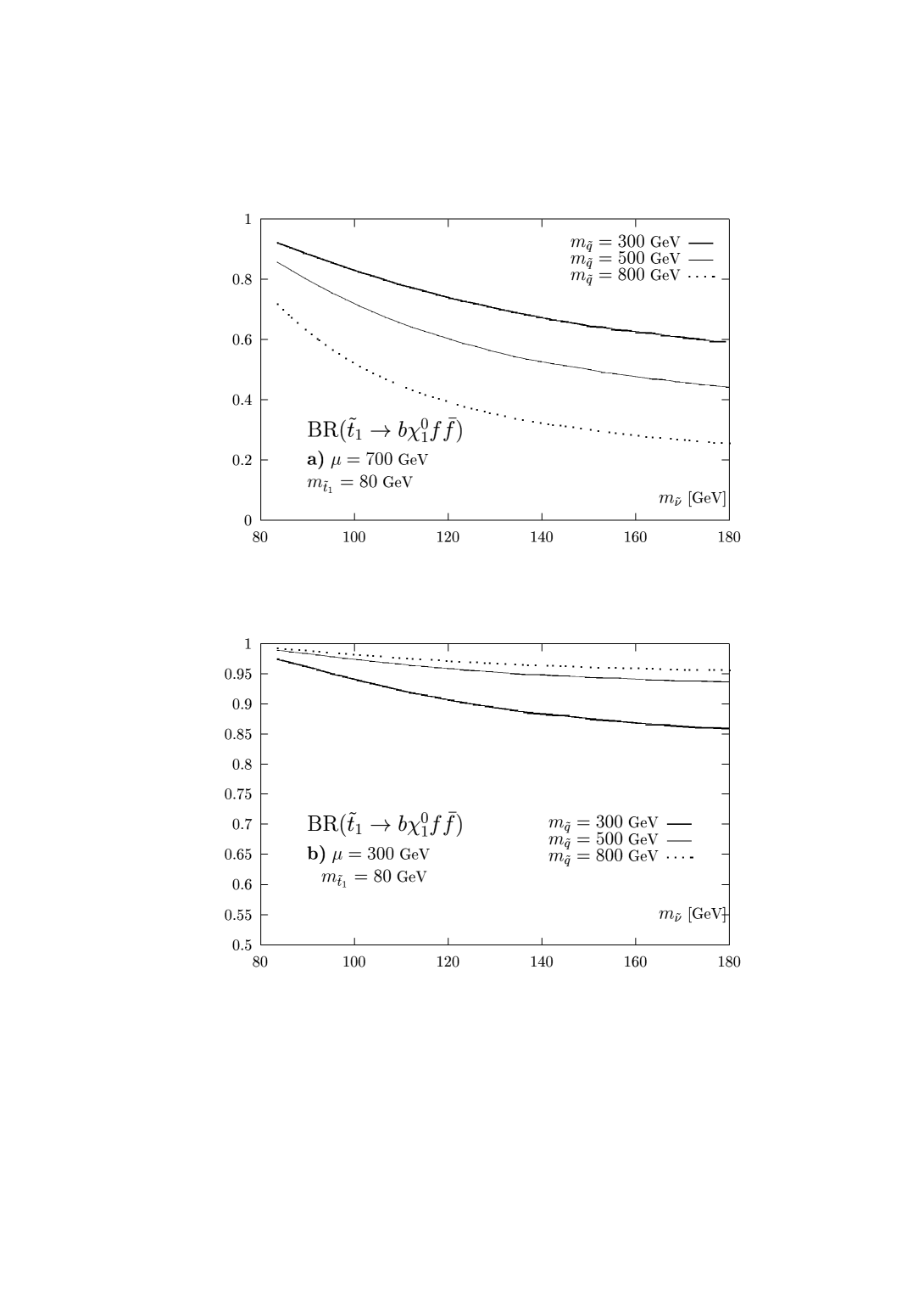
Figure 4: The branching ratio BR$(\tilde{t}_{1}\rightarrow b\chi_{1}^{0}f\bar{f}^{\prime})$ as a function of the sneutrino mass $m_{\tilde{\nu}}$ for a scalar top mass $m_{\tilde{t}_{1}}=80$ and two values of $\mu=700$ GeV (a) and 300 GeV (b).

Figure 5: The branching ratio BR$(\tilde{t}_{1}\rightarrow b\chi_{1}^{0}f\bar{f}^{\prime})$ as a function of stop mass $m_{\tilde{t}_{1}}$ in the mSUGRA scenario for $\mu<0$ (a) and $\mu>0$ (b).

References

- [1] For reviews on the MSSM, see: P. Fayet and S. Ferrara, Phys. Rep. 32 (1977) 249; H.P. Nilles, Phys. Rep. 110 (1984) 1; R. Barbieri, Riv. Nuov. Cim. 11 (1988) 1; R. Arnowitt and Pran Nath, Report CTP-TAMU-52-93; M. Drees and S. Martin, CLTP Report (1995) and hep-9504324; S. Martin, hep-ph9709356; J. Bagger, Lectures at TASI-95, hep-ph/9604232.
- [2] H. E. Haber and G. Kane, Phys. Rep. 117 (1985) 75.
- [3] Particle Data Group, C. Caso et al., Eur. Phys. Journal C3 (1998) 1; for a more recent complilation see for instance, A. Djouadi et al., hep–ph/9901246.
- [4] CDF Collaboration, Phys. Rev. D56 (1997) R1357; D0 Collaboration, contribution to the EPS–HEP Conference, Jerusalem 1997, Ref. 102.
- [5] F. Cerutti, Report from the LEP SUSY working group, talk given on behalf of the LEP SUSY working group, LEPC, 15 sept. 1998.
- [6] J. Ellis and S. Rudaz, Phys. Lett. B128 (1983) 248; M. Drees and K. Hikasa, Phys. Lett. B252 (1990) 127.
- [7] For recent reviews of the two–body decays of top squarks, see A. Bartl et al., hep–ph/9709252; W. Porod, hep-ph/9804208; S. Kraml, hep-ph/9903257; T. Plehn, hep-ph/9809319.
- [8] P. Fayet, Phys. Lett. 69B (1977) 489.
- [9] K.I. Hikasa and M. Kobayashi, Phys. Rev. D36 (1987) 724.
- [10] G. Kane and J.P. Leveille, Phys. Lett. 112B (1982) 227; P.R. Harrison and CH. Llewellyn–Smith, Nucl. Phys. B213 (1983) 223; E. Reya and DP. Roy, Phys. Rev. D32 (1985) 645; S. Dawson, E. Eichten and C. Quigg, Phys. Rev. D31 (1985) 1581; H. Baer and X. Tata, Phys. Lett. 160B (1985) 159; W. Beenakker, M. Krämer, T. Plehn, M. Spira and P.M. Zerwas, Nucl. Phys. B515 (1998) 3.
- [11] H. Baer and X. Tata, Phys. Lett. 167B (1986) 241; H. Baer, M. Drees, R. Godbole, J. Gunion and X. Tata, Phys. Rev. D44 (1991) 725; M. Borzumati and N. Polonsky, hep-ph/9602433; A. Djouadi, W. Hollik and C. Jünger, Phys. Rev. D54 (1996) 5629; C.S. Li, R. J. Oakes and J. M. Yang, Phys. Rev. D54 (1996) 6883.
- [12] CDF Collaboration, Abstract 652, Conference ICHEP98, Vancouver, July 1998.
- [13] For a review see, E. Accomando et al., Phys. Rept. 229 (1998) 1; A. Bartl et al., Z. Phys. C76 (1997) 549; J. Schwinger, “Particles, Sources and Fields”, Addison-Wesley Reading, MA, 1973; M. Drees and K. Hikasa, in Ref. [6]; A. Arhrib, M. Capdequi-Peyranere and A. Djouadi, Phys. Rev. D52 (1995) 1404; H. Eberl, A. Bartl and W. Majerotto, Nucl. Phys. B472 (1996) 481; W. Beenakker, R. Hopker and P.M. Zerwas, Phys. Lett. B378 (1996) 159; W. Beenakker, R. Hopker, T. Plehn and P.M. Zerwas, Z. Phys. C75 (1997) 349.
- [14] OPAL Collaboration, G. Abbiendi et al., Phys. Lett. B456 (1999) 95.
- [15] W. Porod and T. Wöhrmann, Phys. Rev. D55 (1997) 2907; W. Porod, Phys. Rev. D59 (1999) 095009.
- [16] G. Altarelli and R. Rückl, Phys. Lett. 144B (1984) 126; I. Bigi and S. Rudaz, Phys. Lett. 153B (1985) 335.
- [17] Y. Mambrini, Ph. D. Thesis, in preparation.
- [18] M. Carena et al., Nucl. Phys. B426 (1994) 269; W. de Boer, R. Ehret and D.I. Kazakov, Z. Phys. C67 (1994) 647; M. Drees and S. Martin in [1].
- [19] J.F. Gunion and H.E. Haber, Nucl. Phys. B272 (1986) 1.
- [20] See for instance, G. Altarelli, hep–ph/9611239; J. Erler and P. Langacker, hep–ph/9809352; G.C. Cho et al., hep–ph/9901351.
- [21] M. Drees and K. Hagiwara, Phys. Rev. D42 (1990) 1709; M. Drees, K. Hagiwara and A. Yamada, Phys. Rev. D45 (1992) 1725; P. Chankowski et al., Nucl. Phys. B417 (1994) 101; D. Garcia and J. Solà, Mod. Phys. Lett. A9 (1994) 211; A. Djouadi et al., Phys. Rev. Lett. 78 (1997) 3626.
- [22] R. Kleiss, W.J. Stirling and S.D. Ellis, Comput. Phys. Commun. 40 (1986) 359.